Numerical Simulation of Hydrodynamic Performance of Podded Propulsion under Maneuvering Condition

Abstract

Podded propulsion offers excellent maneuverability without the need for mechanically complex transmission systems. However, the hydrodynamic performance of podded propulsion under maneuvering conditions has not yet been adequately investigated. This study proposes a Reynolds-averaged Navier–Stokes (RANS)-based method to investigate the hydrodynamic performance of pod thrusters under maneuvering conditions. The accuracy of the numerical method is verified based on a comprehensive convergence analysis and experimental comparison. A comparative analysis of the difference in thrust, moment and their coefficients between maneuvering and steady-state conditions is performed. Additionally, the impact of the advance number on the propeller hydrodynamic performance under maneuvering conditions is examined. The results demonstrate that the thrust coefficient and the torque coefficient of the propeller at positive and negative oblique flow angles exhibit asymmetry owing to the influence of the incoming flow velocity. Furthermore, the thrust and torque under maneuvering conditions increase significantly compared with those under the steady-state condition.

1. Introduction

Podded propulsion is an uncommon propulsion system. In contrast to conventional propulsion, podded propulsion combines the propeller and pod into a single propulsion unit. Because the pods do not require a complex mechanical transmission device, their transmission efficiency is typically higher than that of a conventional rudder propeller unit. Pod propulsion enables full utilization of electric propulsion systems, resulting in pod propulsion units with a wide range of applications. In addition, the mechanical structure of pod propulsion is relatively simple and offers many advantages, such as vibration damping and a flexible internal design layout. Pod propellers rotate freely and can generate thrust in any direction, which provides excellent maneuverability to the ship. However, the hydrodynamic performance of the pod propellers under maneuvering and steady-state conditions differs significantly. Therefore, it is necessary to investigate the maneuvering performance of the propellers and pods at different angles.

Early research on pods focused on direct current conditions, particularly the interaction between the pod and propeller, and the hydrodynamic performance of the propeller. Bal [1] analyzed the flow around a pod unit and the performance characteristics of the propeller on the pod. Wang et al. [2] examined the influence of hydrodynamic performance on design parameters such as the axial distance between the front and rear propellers and the advanced speed ratio. Sánchez et al. [3] coupled a Reynolds-averaged Navier–Stokes (RANS) solver with a single-phase cavitation model, which can reasonably predict the degree of cavitation without significantly increasing the computational effort. Xiong et al. [4] used the unsteady panel method to solve the hydrodynamic performance of towed podded propulsion and calculated the hydrodyjmse-2271037 namic performance of podded propulsion in uniform and non-uniform inflows. Zhao et al. [5] developed a set of hydrodynamic performance measurement devices based on the structural characteristics of an L-shaped pod propulsion. Islam et al. [6] combined an experimental evaluation with a numerical prediction to study the hydrodynamic performance of podded propulsion. Cao et al. [7] studied the influence of the initial phase angle and load matching of the podded propulsion through a multi-scheme model test of the podded propeller. Shamsi et al. [8] used a turbulent numerical simulation method to analyze the hydrodynamic performance of podded propulsion in open-water and azimuth conditions. In addition, a RANS-based solver was used to study the changes, at different angles, in the hydrodynamic properties of the podded propulsion.

In oblique flow, the hydrodynamic performance changes significantly. In particular, under instantaneous slewing conditions, the hydrodynamic performance changes are particularly dramatic. Xie et al. [9] employed an experimental method to measure the thrust, torque, and steering torque at multiple azimuth angles for towed pod thrusters. The test data will facilitate the design of ship maneuvering gear and podded thrusters. Xu et al. [10] adopted a numerical simulation method and researched the relationship between the hydrodynamic performance parameters and steering angle of the hybrid CRP-podded propulsion. Liu et al. [11] employed a panel method to predict the unsteady force, torque, and bending torque of podded propulsion systems at different azimuth angles. Shen et al. [12] used an experimental method to study the cavitation performance of a podded thruster in the range of rudder angle (±5°). At the same time, they measured the pulsating pressure on the hull and the pod at 0° rudder angle. This verifies the design and application of the podded thruster. Reichel [13] applied an experimental method to investigate the hydrodynamic characteristics of a podded thruster in open water over a range of forwarding coefficients from 0.0 to 0.8 and deflection angles in the range of ±45°. Andreas et al. [14] applied the unsteady RANS solver to calculate the forces and torque of podded propulsion. Then, they compared their results with those of the conventional propeller, and discussed their maneuverability performance at design speeds. Stettler et al. [15] employed an experimental method to demonstrate the stress problem of podded propulsion and analyzed the relationship between the stress and azimuth angle of the propeller under different advanced coefficients. Their method reduced the propeller surface pressure by improving the azimuth angle, which reduces propeller loss. Islam et al. [16] applied an experimental method to discuss the propulsion characteristics of pods under static and dynamic azimuth conditions. The results showed that the propeller load and propulsion performance of the pod and propeller had a significant relationship with the azimuth angle. Amini et al. [17] performed RANS-based numerical simulation to investigate the influence of a wide range of oblique flow angles on the hydrodynamic performance of the propeller under two different loading conditions.

The pod propulsion system comprises a propeller and pod. This structure allows the entire pod to rotate 360°, which enables pod propulsion to deliver improved maneuverability over that of a conventional propeller rudder system. Therefore, it is important to study the hydrodynamic performance of podded propulsion under maneuvering conditions. Islam et al. [18] adopted an experimental method to study the axial thrust and torque, unit thrust, and lateral force of the podded propulsion in maneuvering conditions in the range of ±180°. Akinturk et al. [19] applied an experimental method to study the performance of pods under different maneuvering conditions in the range of ±180° and investigate the influence of hydrodynamic performance of podded propulsion under static and dynamic conditions. Shen et al. [20] established a numerical model and used a slip grid to simulate the hydrodynamic performance of a podded propulsion in an unstable flow. The predicted results were consistent with the experimental data, validating the feasibility of the model technology. Islam et al. [21] used computational fluid dynamics (CFD) simulation to study the hydrodynamic performance of podded propulsion under various extreme static azimuth conditions. The analysis shows that the RANS-based method can predict the performance of the podded propulsion under extreme azimuth and high-load conditions, and its accuracy is of the same order of magnitude as the experimental results. Zhao et al. [22] used the RANS method and SST k–ω turbulence model to study the loads on podded propulsion. The hydrodynamic characteristics of podded propulsion under azimuth angle were analyzed, and the changes in propeller thrust and torque were investigated. Mewis et al. [23] adopted an experimental method to study the hydrodynamic efficiency of podded propulsion under maneuvering conditions. Their experiments show that podded propulsion has lower propulsion efficiency than the traditional single propeller. Ortolani et al. [24,25,26] used experimental and numerical simulation methods to study the periodic evolution of single-blade load and propeller load at the rear of the ship under different operating conditions, as well as the effects of factors such as ship wake and different oblique flow angles on propeller load, pressure pulsation, noise, and other aspects. Reichel M et al. [27,28,29] used numerical simulation and experimental methods, the experimental process complies with the implementation procedures for maneuvering tests proposed by the International Maritime Organization (IMO). Validation shows acceptable agreement between numerical and experimental results, i.e., confirms the usability of developed mathematical model to identify the trends in performance also for course unstable ship.

These studies have not adequately investigated the hydrodynamic performance of pods under maneuvering conditions. However, this is a key problem in pod propulsion research, and further investigation is required. There is limited understanding of the hydrodynamic performance of the propeller under maneuvering conditions because the interaction between the propeller and pod shell remains difficult to predict. However, in this study, numerical simulation is performed using the STAR-CCM+ software to analyze the forces and torques of the propeller blade under maneuvering and steady-state conditions. Moreover, the relationship between the propeller hydrodynamic performance and water incidence angle is determined.

2. Governing Equations

Under the assumption that the fluid has a constant density, is incompressible, and is devoid of mass forces, the continuity equation of a Newtonian fluid takes the following form:

$$\frac{\mathit{\partial }{\mathit{u}}_{\mathit{i}}}{\mathit{\partial }{\mathit{x}}_{\mathit{i}}}=\mathbf{0}$$

(1)

$$\frac{\mathit{\partial }{\mathit{u}}_{\mathit{i}}}{\mathit{\partial }\mathit{t}}+\frac{\mathit{\partial }}{\mathit{\partial }{\mathit{x}}_{\mathit{j}}}({\mathit{u}}_{\mathit{i}}{\mathit{u}}_{\mathit{j}}) =-\frac{\mathbf{1}}{\mathit{\rho }}\frac{\mathit{\partial }\mathit{p}}{\mathit{\partial }{\mathit{x}}_{\mathit{i}}}+\mathit{v}\frac{\mathit{\partial }}{\mathit{\partial }{\mathit{x}}_{\mathit{i}}}\left[\frac{\mathit{\partial }{\mathit{u}}_{\mathit{i}}}{\mathit{\partial }{\mathit{x}}_{\mathit{j}}}+\frac{\mathit{\partial }{\mathit{u}}_{\mathit{j}}}{\mathit{\partial }{\mathit{x}}_{\mathit{i}}}\right]$$

(2)

where ${\mathit{u}}_{\mathit{i}}$ (i = 1, 2, 3) is the velocity component;${\mathit{x}}_{\mathit{i}}$ (i = 1, 2, 3) are the coordinates; P is the pressure (Pa); v is the viscosity coefficient of fluid motion (${\mathrm{m}}^2{\mathrm{s}}^{-1}$); $\mathit{\rho }$ is the fluid density (kg/m³); and t is time (s). These are the basic governing equations used in CFD. The variables in Equation (2) are decomposed into time averages and pulsations for the simulation of turbulent motion as follows.

$$\varnothing =\overline{\varnothing }+{\varnothing }^{\prime }$$

(3)

Then, by averaging the time on both sides of Equation (2), we obtain the Navier–Stokes equation of the time average.

$$\frac{\mathit{\partial }{\mathit{u}}_{\mathit{i}}}{\mathit{\partial }\mathit{t}}+\frac{\mathit{\partial }}{\mathit{\partial }{\mathit{x}}_{\mathit{j}}}({\mathit{u}}_{\mathit{i}}{\mathit{u}}_{\mathit{j}}) =-\frac{\mathbf{1}}{\mathit{\rho }}\frac{\mathit{\partial }\mathit{p}}{\mathit{\partial }{\mathit{x}}_{\mathit{i}}}+\mathit{v}\frac{\mathit{\partial }}{\mathit{\partial }{\mathit{x}}_{\mathit{i}}}\left[\frac{\mathit{\partial }{\mathit{u}}_{\mathit{i}}}{\mathit{\partial }{\mathit{x}}_{\mathit{j}}}+\frac{\mathit{\partial }{\mathit{u}}_{\mathit{j}}}{\mathit{\partial }{\mathit{x}}_{\mathit{i}}}\right]+\frac{\mathit{\partial }}{\mathit{\partial }{\mathit{x}}_{\mathit{j}}}\left[\overline{-{\mathit{u}}_{\mathit{i}}^{\mathit{\prime }}{\mathit{u}}_{\mathit{j}}^{\mathit{\prime }}}\right]$$

(4)

In Equation (4), ${\mathit{u}}_{\mathit{i}}$,${\mathit{u}}_{\mathit{j}}$, and p is the time average, and we add the Reynolds stress term $\frac{\mathit{\partial }}{\mathit{\partial }{\mathit{x}}_{\mathit{j}}}\left[\overline{-{\mathit{u}}_{\mathit{i}}^{\mathit{\prime }}{\mathit{u}}_{\mathit{j}}^{\mathit{\prime }}}\right]$. We use a turbulence model to solve the turbulence problem of viscous fluids.

2.1. RANS Equations

By utilizing the time-averaged equation, the RANS equations can account for the transient pulsating momentum. The primary objective of these equations is not to solve the transient Navier–Stokes equations directly but to develop an approach to solve the time-averaged turbulence equations. The RANS equations represent the governing equations for the average variables of the flow field. They assume that the turbulence-induced variation in the flow field variable consists of a time-averaged quantity and a fluctuating quantity. The Boussinesq hypothesis is then introduced, which postulates that the turbulent Reynolds stress is proportional to the strain. This enables the turbulence calculation to be reduced to the calculation of the proportional coefficient between the Reynolds stress and the strain. According to Guo et al. [30], the RANS turbulence model establishes a strong connection with the RANS equations, which govern the mean flow characteristics. The equations for average mass and momentum transfer can be expressed in the following form:

$$\frac{\mathit{\partial }\mathit{\rho }}{\mathit{\partial }\mathit{t}}+\frac{\mathit{\partial }}{\mathit{\partial }{\mathit{x}}_{\mathit{i}}}\left(\mathit{\rho }{\mathit{u}}_{\mathit{i}}\right)=\mathbf{0}$$

(5)

$$\frac{\mathit{\partial }}{\mathit{\partial }\mathit{t}}\left(\mathit{p}{\mathit{u}}_{\mathit{i}}\right)+\frac{\mathit{\partial }}{\mathit{\partial }{\mathit{x}}_{\mathit{j}}}\left(\mathit{\rho }{\mathit{u}}_{\mathit{i}}{\mathit{u}}_{\mathit{j}}\right)=\frac{\mathit{\partial }\mathit{p}}{\mathit{\partial }{\mathit{x}}_{\mathit{j}}}+\frac{\mathit{\partial }}{\mathit{\partial }{\mathit{x}}_{\mathit{j}}}\left(\mathit{\mu }\frac{\mathit{\partial }{\mathit{u}}_{\mathit{i}}}{\mathit{\partial }{\mathit{x}}_{\mathit{j}}}\mathit{-}\mathit{\rho }\overline{{\mathit{u}}_{\mathit{i}}^{\mathit{\prime }}{\mathit{u}}_{\mathit{j}}^{\mathit{\prime }}}\right)+{\mathit{s}}_{\mathit{j}}$$

(6)

In all the equations, ${\mathit{u}}_{\mathit{i}}$ denotes the time-averaged value of the velocity component, t is the time, $\mathit{p}$ is the time-averaged value of the pressure, $\mathit{\rho }$ is the fluid density, $\mathit{\mu }$ is the dynamic viscosity coefficient, $\mathit{\rho }\overline{{\mathit{u}}_{\mathit{i}}^{\mathit{\prime }}{\mathit{u}}_{\mathit{j}}^{\mathit{\prime }}}$ denotes the Reynolds stress term, and ${\mathit{s}}_{\mathit{j}}$ denotes the generalized source term of the momentum equation.

2.2. Turbulence Model

We performed simulations using the SST k–ω turbulence model, which considers the flow characteristics of the inverse pressure gradient boundary layer and retains the advantage of the turbulence model calculation. The transport equation for the turbulence model is expressed as follows:

$$\frac{\partial \left(\rho k\right)}{\partial t}+\nabla \cdot (\rho k\bar{v})=\nabla \cdot \left[\left(\mu +{\sigma }_k{\mu }_t\right)\nabla k\right]+P_k-\rho {\beta }^{*}{f}_{{\beta }^{*}}\left(\omega k-{\omega }_0{k}_0\right)+S_k$$

(7)

$$\frac{\partial \left(\rho \omega \right)}{\partial t}+\nabla \cdot (\rho \omega \bar{v})=\nabla \cdot \left[\left(\mu +{\sigma }_{\omega }{\mu }_t\right)\nabla \omega \right]+P_{\omega }-\rho \beta f_{\beta }\left({\omega }^2-{\omega }_0^2\right)+S_{\omega }$$

(8)

where $\bar{\mathit{v}}$ is the average velocity, $\mathit{\mu }$ is the dynamic viscosity, ${\mathit{\sigma }}_{\mathit{k}}$, ${\mathit{\sigma }}_{\mathit{\omega }}$, ${\mathit{\alpha }}^{*}$, ${\mathit{C}}_{\mathit{T}}$, ${\mathit{a}}_{\mathbf{1}}$ is the model coefficient, ${\mathit{P}}_{\mathit{k}}$ and ${\mathit{P}}_{\mathit{\omega }}$ are the result items, ${\mathit{f}}_{{\mathit{\beta }}^{*}}$ is the correction factor for free shear, ${\mathit{f}}_{\mathit{\beta }}$ is the eddy current extension correction factor, ${\mathit{S}}_{\mathit{k}}$ and ${\mathit{S}}_{\mathit{k}}$ is the customized source items, ${\mathit{k}}_{\mathbf{0}}$ and ${\mathit{\omega }}_{\mathbf{0}}$ are the ambient turbulence values to prevent turbulence decay, and S is the modulus of the average strain rate tensor.

3. Computational Domain and Grid Conditions

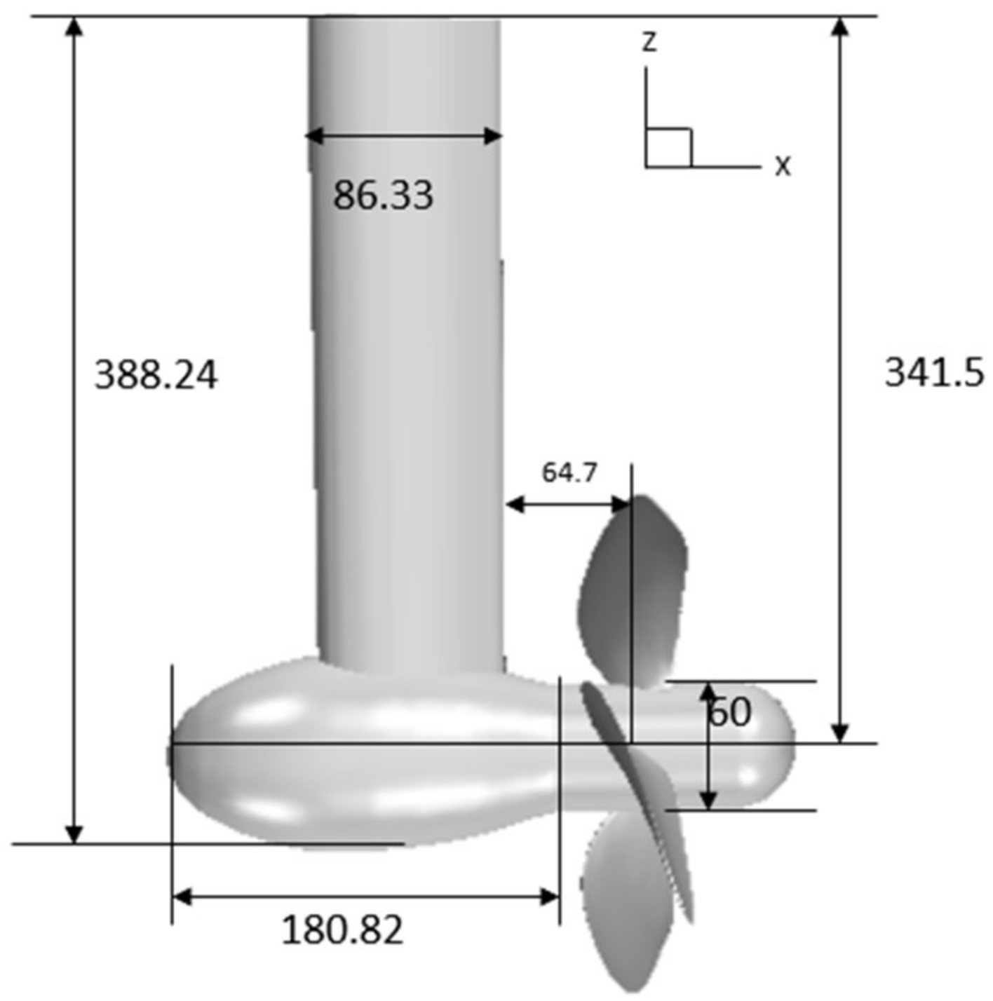
The pod unit used in this study is the P-1374 standard propeller designed by MARINTEK. This unit includes three parts: propeller, pod, and bracket.

Table 1. Main parameters of the propeller.

Parameter	Value
Propeller diameter	250 mm
Hub diameter	60 mm
Pitch ratio P/D	1.1
Pitch angle	25°
Area ratio	0.6
Number of blades	4

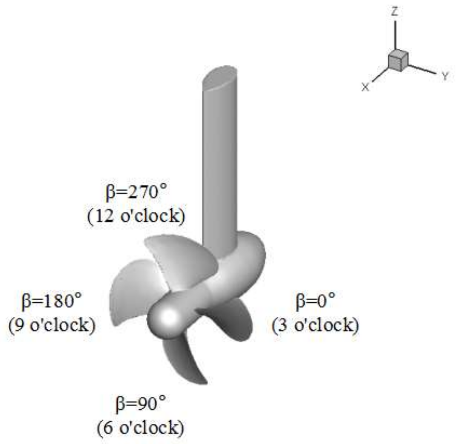
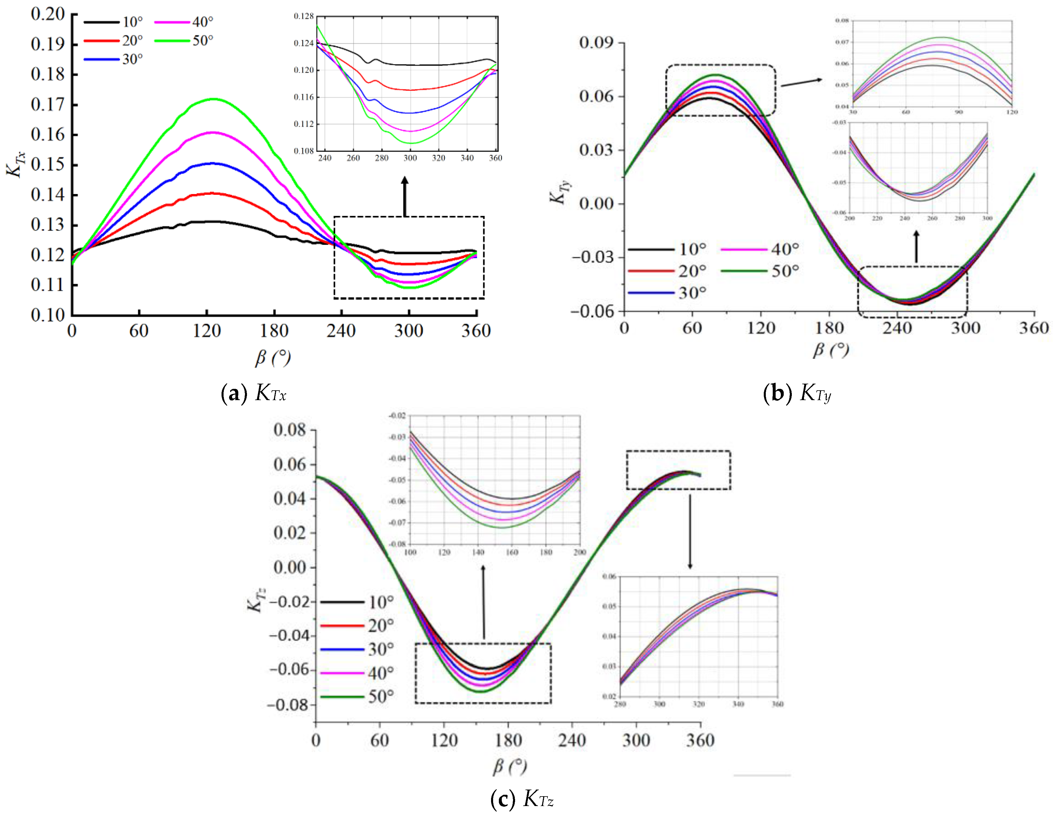
lists the geometric parameters of the propeller. This structure is modeled using Siemens NX, a 3D modeling software. The structure obtained from the work by Zhao et al. [19]. Where the diameter of the propeller was 250 mm, and the diameter of the hub was 60 mm. Figure 1 shows the geometric dimensions of each part except for the blade. Figure 2 shows a geometric model of the paddle. In Figure 2, $\beta$ is the rotation angle of a single blade; the three o’clock direction is defined as the 0° position of the blade, and the 90°, 180°, and 270° positions are defined in turn along the rotation direction of the blade.

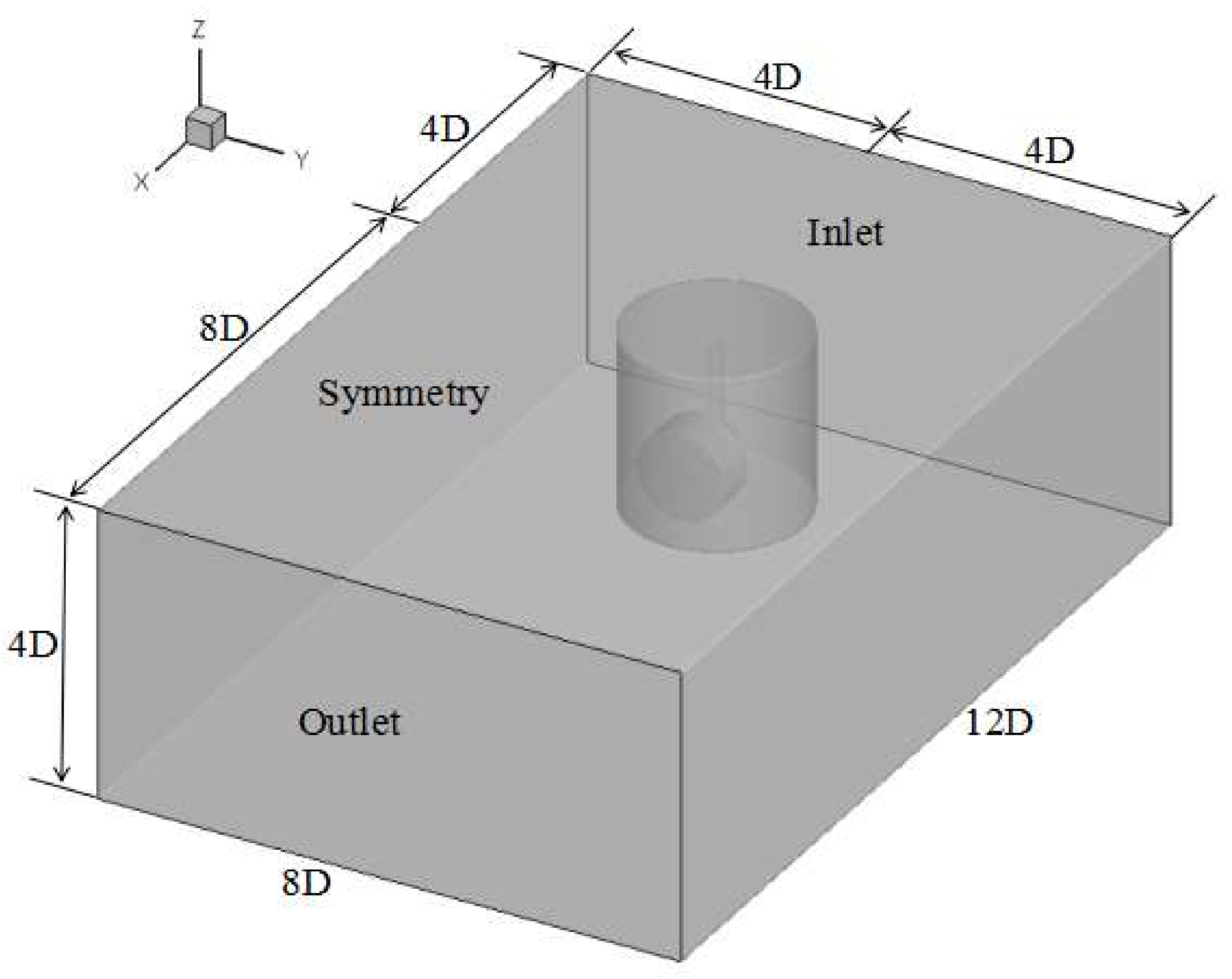
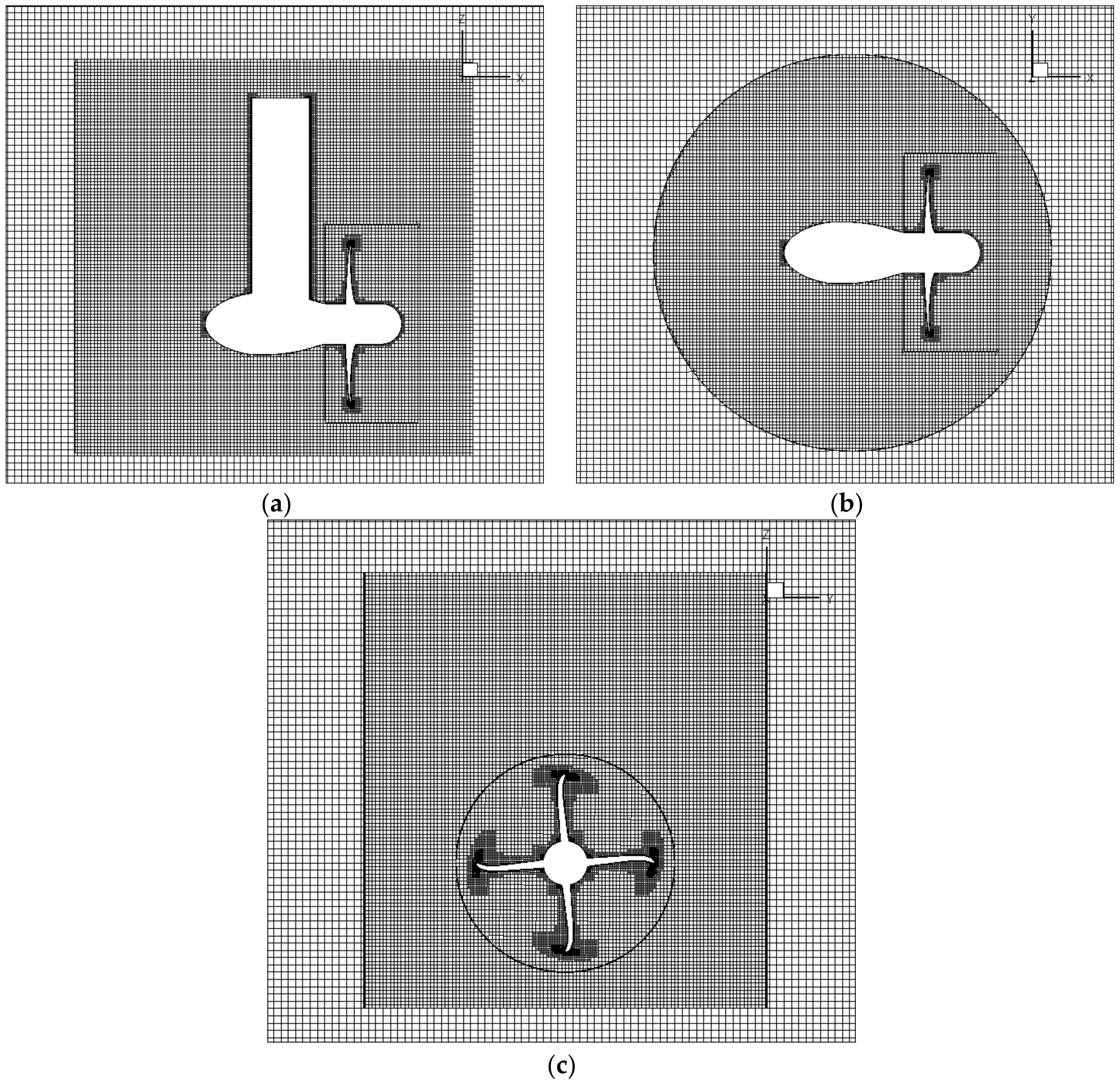
Figure 3 shows the propeller diameter and the length, width, and height of the computational domain are 12D, 8D, and 4D, respectively. The boundary condition for the inlet is set to the velocity inlet, the boundary condition for the outlet is set as the pressure outlet, and the boundary conditions of the surrounding planes of the computational domain are set to symmetry.

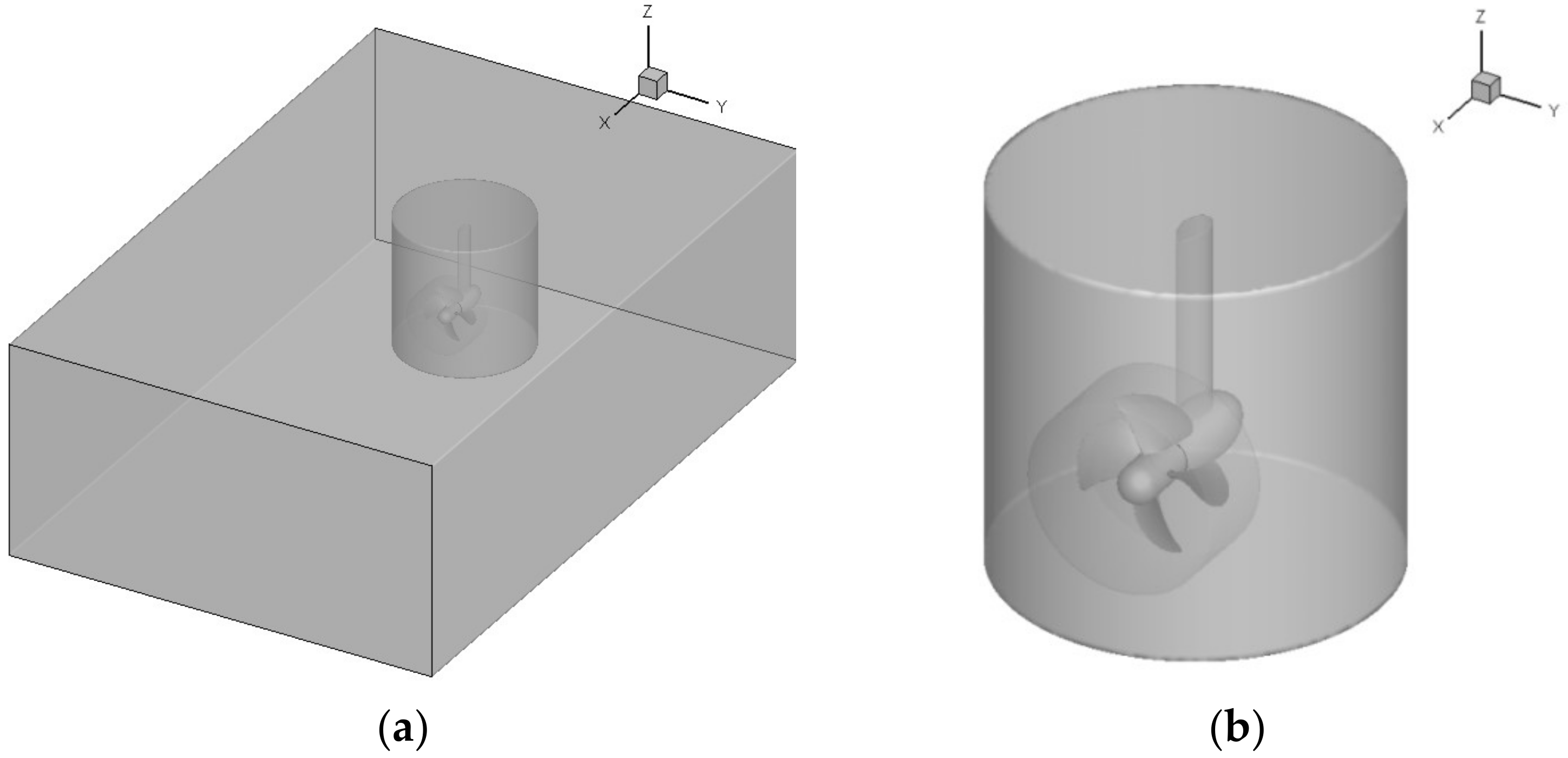
Figure 4 shows a part of the rotation domain; the simulation uses the sliding mesh method to simulate the rotational motion. The simulation sets up two rotation domains. The small rotation domain includes the propeller, and the function is to simulate the motion of the propeller. The large rotation domain includes the pod, the bracket, and the small rotation domain, and the function is to simulate the maneuvering motion of the pod unit. The small rotation domain is located within the large rotation domain and moves with the large rotation domain.

4. Grid Validation

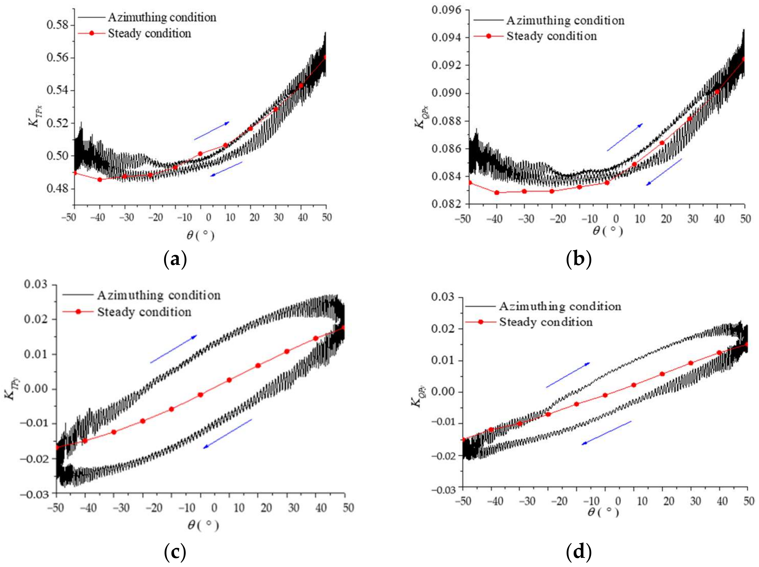
Figure 5 lists the two oblique flow conditions discussed in the study; one is the maneuvering condition, which calculates the transient load, and the other is the steady-state condition, which calculates the steady-state load. The turning angular velocity of the maneuvering condition is not zero, while the turning angular velocity of the steady-state condition is zero. VA is a uniform flow along the positive X-axis, $\theta$ is the angle between the propeller and OX axes. The positive direction of the Y-axis is defined as −90° and the negative direction of the Y-axis is defined as 90°, that is, clockwise rotation is positive. The positive direction of the Y-axis points to the ships starboard side, and the negative direction points to the port side. O-X-Y is the stationary coordinate system, and o-x-y is the rotating coordinate system. The origin of the O-X-Y coordinate is at the center of the top of the bracket, and the origin of the o-x-y coordinate is at the center of the paddle. The o-x-y coordinate system moves with the propeller, and the o-x direction is always the propeller axis.

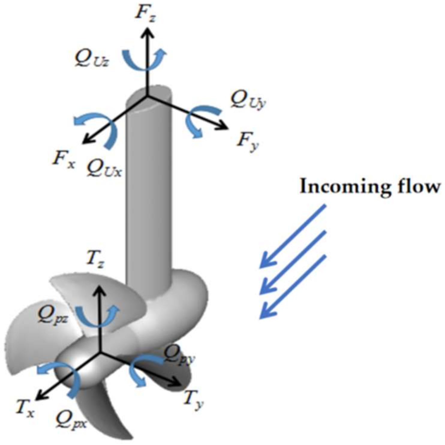
Figure 6 shows a schematic of the load on the pod unit where T_x, T_y, and T_z, are the thrust of the propeller in the axial, lateral, and vertical directions of the propeller. Q_px, Q_py, and Q_pz are the moment of the propeller in the axial, lateral, and vertical torques of the propeller, respectively. F_x, F_y, and F_z are rotational angular velocity, respectively. The load on the propeller is fixed in the o-x-y rotating coordinate system, and the load on the pod unit is fixed in the O-X-Y stationary coordinate system.

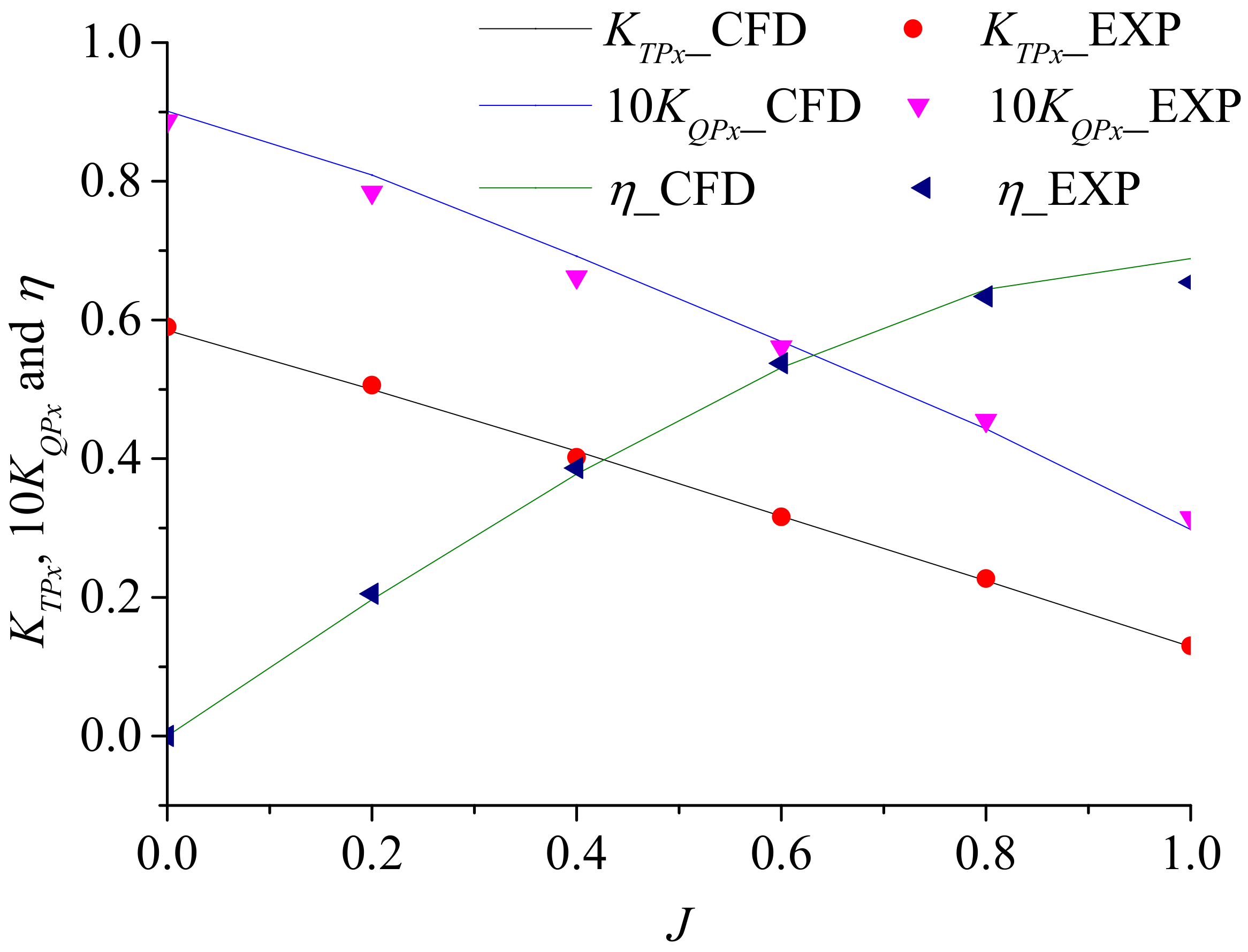
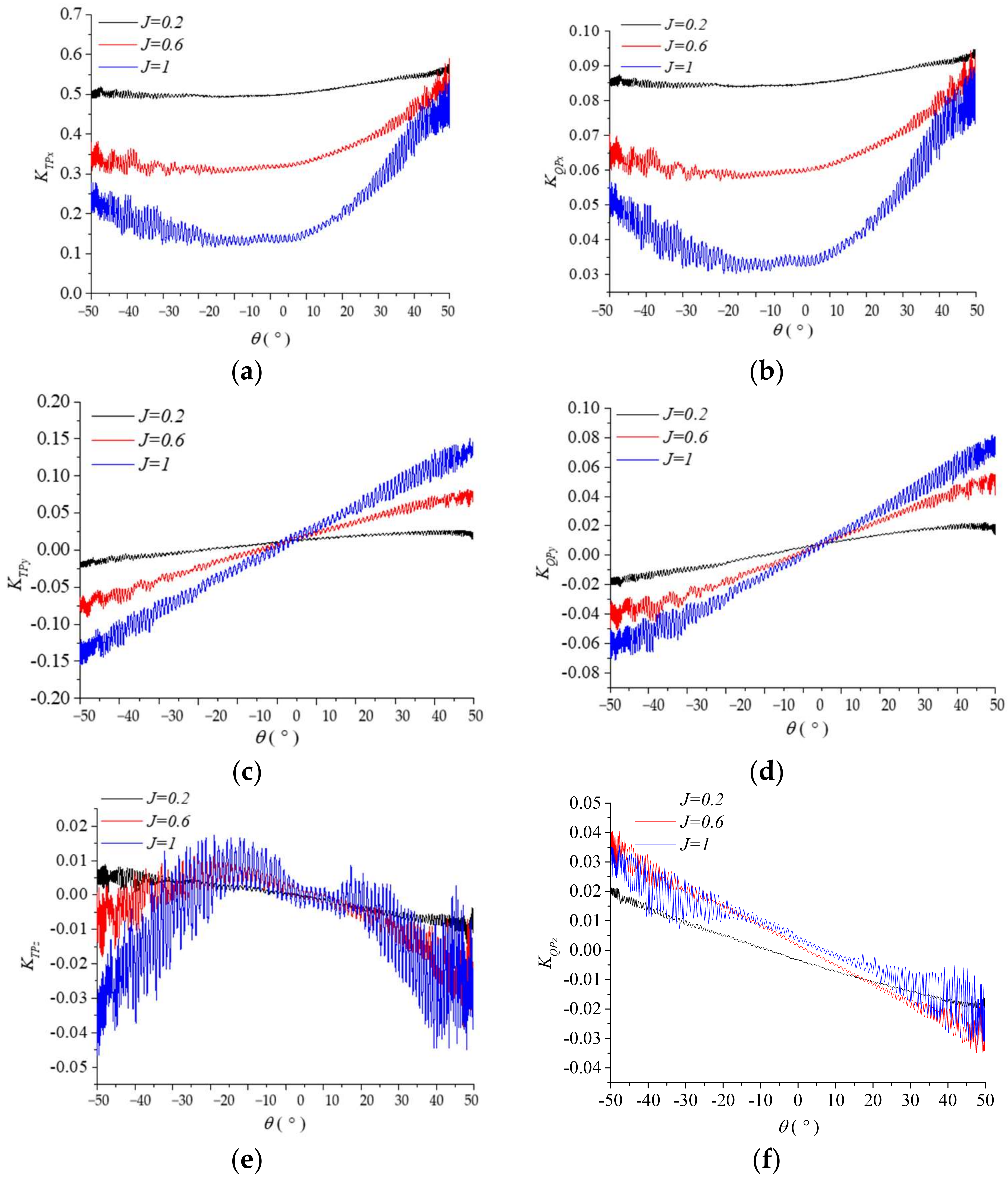
The thrust coefficient of the propeller is K_TP, the torque coefficient of the propeller is K_QP, and they are expressed as follows:

$$K_{TPi}=\frac{T_i}{\rho n^2{D}^4}$$

(9)

$$K_{QPi}=\frac{Q_{pi}}{\rho n^2{D}^5}$$

(10)

$$\eta =\frac{J}{2\pi }\frac{K_T}{K_Q},J=\frac{V_A}{nD}$$

(11)

where $\rho$ is the density of the fluid, n is the speed of the propeller (10 rps), D is the diameter of the paddle, $\eta$ is the propulsion efficiency, J is the advance number, and the change in its value is caused by the change in V_A.

4.1. Mesh Convergence Analysis

The number of grids significantly influences the calculation results in the numerical simulation. According to the work of Hu et al. [31], we set three grid schemes before the grid convergence analysis. The basic size of the coarse grid is 0.005 m, and the medium and coarse grids are 0.0063 and 0.0079 m, respectively. Figure 7 shows the surface of the fine grid. In Figure 7a, the grids of the blades and hub are densified. Higher requirements for grid quality are due to a faster blade tip speed; therefore, the blade tip mesh is further refined, as shown in Figure 7b. Figure 8 shows the fluid domain grid of the fine grid.

Table 2. Convergence analysis of the grid numbers.

Mesh	Number of Elements	EXP		CFD
		KTPx	10KQPx	KTPx	Error	10KQPx	Error
Coarse Grid	4 M	0.5058	0.7842	0.4888	3.34%	0.8173	6.31%
Medium Grid	6.5 M			0.4995	1.24%	0.8337	3.28%
Fine Grid	8 M			0.5002	1.11%	0.8092	3.19%

lists the thrust and torque coefficients of the propeller under three grid conditions. The time step corresponds to the time that the propeller rotated 1°. The experimental data were obtained from the work conducted by Zhao et al. [22]. The simulation in Table 2 selects the steady-state conditions. The inlet velocity coefficient selected was J = 0.2, and the oblique flow angle was 0°. The results show that, as the grid size decreases, the error in the thrust coefficient K_TPx decreases. The error is only 1.11% under the fine grid conditions. The error of the torque coefficient K_QPx is reduced as the grid size decreased; it is least at 3.19% for the fine grid condition. 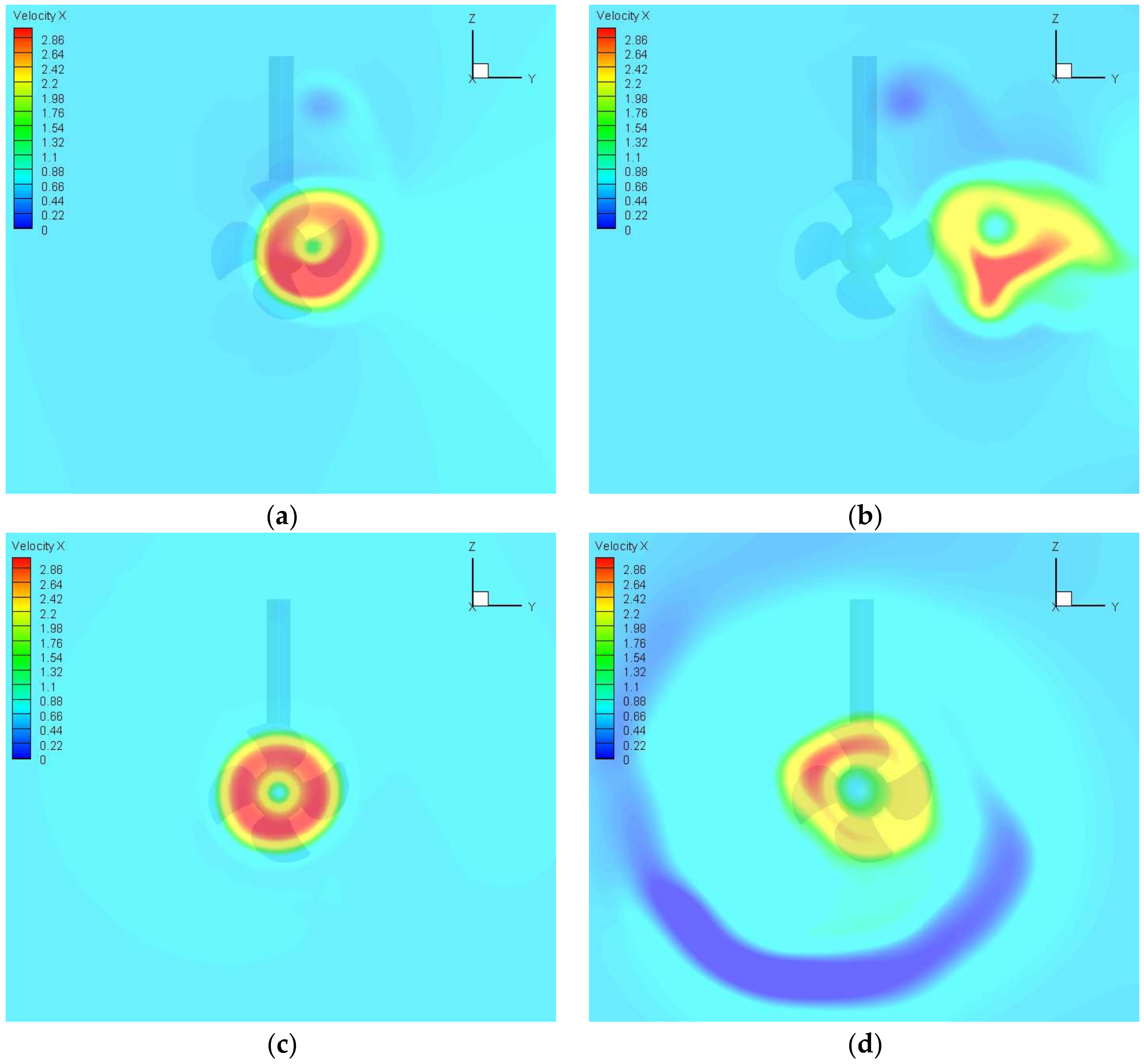Figure 9 shows the pressure distribution of the propeller for the medium and fine grids. From the area marked by the circles in Figure 9a, it can be seen that both medium and fine grids clearly demonstrate the flow phenomenon and turbulence characteristics of the paddle surface. We selected the medium grid for the next step because the fine grid took too long to compute and required considerable amount of computational resources. Cp, the pressure coefficient, is defined as follows:

$$Cp=\frac{p}{0.5\rho U^2}$$

(12)

where $p$ is the pressure and U is the linear velocity at the propeller tip.

4.2. Hydrodynamic Performance of the Podded Propeller

Figure 10 shows a comparison of the hydrodynamic loads between the numerical and test results. The numerical simulation, shown in Figure 10, selects the steady-state condition, the oblique flow angle of 0°, and the selected advance number range of J = 0.0~1.0. The numerical calculation results are consistent with the experimental results. Choosing J = 0.2 (working condition selected in this study), the errors of the thrust coefficient, torque coefficient, and propulsion efficiency of the propeller are all below 5%. Thus, the results validate our choice of using the RANS approach in this study.

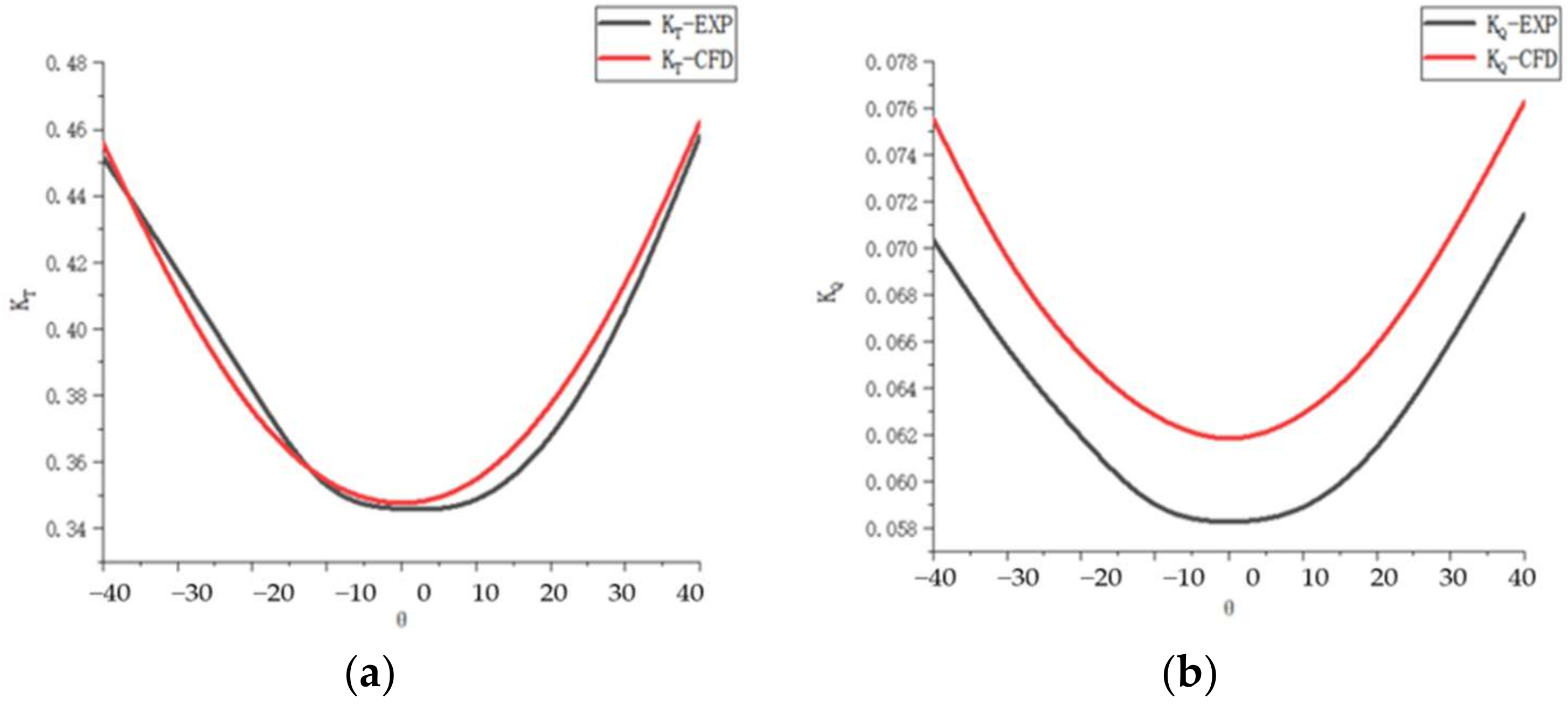
Figure 11 is the comparison between the numerical simulation and the experiment under the towed conditions of podded propeller, and the steering angle of podded propulsor is from −40° to 40°, with the interval of 10°; there are a total of nine working conditions. Choosing J = 0.6, the rotational speed of the propeller is 10 rps, the inlet velocity is 0.9 m/s. The data of the experimental part come from the work carried out by XU J et al. [10]. It can be observed from the figure that in the numerical simulation and experiment, the relative error of propeller thrust coefficient is within 3%, and the relative error of torque coefficient is mostly less than 7%.

5. Results and Discussion

5.1. Overall Load

Figure 12 shows the propeller load variation for pod propulsion at the three advance numbers under maneuvering conditions. The process of turning the pod unit from the starboard to the port is selected. The rotational speed of the propeller is 10 rps and the motion function of the pod unit is calculated as follows:

$$\omega =\frac{{\pi }^2}{12}cos(0.3\pi t)$$

(13)

where $\omega$ is the angular velocity of the pod unit swinging in the X-Y plane, the motion period is $\frac{20}{3}s$. The movement range of the pod unit is −50° to 50°. The angular velocity has a maximum value of 0° and the angular velocity is 0 at ±50°.

Figure 12a,b shows the thrust coefficients curve K_TPx and the torque coefficients curve K_QPx in the paddle X-direction, respectively. The value of K_TPx is a minimum value at 0°, which increases gradually on both sides, and reaches a maximum value at ±50°. However, the value at 50° is greater than the value at −50°, which is due to the effect of propeller steering causing the load at symmetrical angles not to be symmetrical. At the same oblique flow angle, it appears that with the increase in the advance number, K_TPx gradually decreases; the difference of K_TPx is the largest at 0° for different advance numbers, while the difference is the smallest at ±50°. We see that the fluctuation of the curve is more severe at ±50°, owing to the enhanced lateral impact of the incoming flow on the propeller at high slope flow angle conditions, which leads to a more complex turbulence pulsation and larger fluctuations in the propeller load.

Figure 12c,d shows the thrust coefficients K_TPy and the torque coefficients K_QPy in the paddle Y-direction, respectively. With the increase in oblique flow angle, the value of K_TPy increases. When J = 1.0, its load curve increases faster than the others do. The variation of the intersect when the oblique flow angle is 5°, between −50° and 5°, J = 1.0, the value of K_TPy is minimal, between 5° and 50°, J = 1.0, the value of K_TPy is maximum. This indicates that the higher the incoming flow velocity, the greater the Y-direction load on the propeller.

Figure 12e,f shows the thrust coefficients K_TPz and the torque coefficients K_QPz in the paddle Z-direction, respectively. When J = 0.2, the value of K_TPz decreases with the increase in the oblique flow angle. However, at J = 0.6 and 1.0, the impact of the incoming flow on the paddle front bracket is enhanced. This leads to a sharp fluctuation in the curve of K_TPz. The value of the K_QPz decreases with the oblique flow angle increase; when J = 0.2, its value is slightly smaller. Normally, the values of K_QPz are not different in the three advanced number conditions.

Figure 13 shows a comparison of the hydrodynamic loads of the propeller under steady-state and maneuvering conditions, where the blue arrow in the figure shows the direction of movement of the pod unit. Figure 13a,b shows the thrust coefficient K_TPx curve and the torque coefficient K_QPx curve in the X-direction of the propeller, respectively. Under maneuvering conditions, the propeller X-direction load of the pod unit is slightly greater when the pod unit is turned from starboard to port than when it is turned from port to starboard. At a positive oblique flow angle, the propeller load under steady state and under maneuvering conditions is similar; however, it differs greatly at a negative diagonal flow angle. When the oblique flow angle is −50°, the average value of K_QPx under the maneuvering condition is 0.086, while the value under the steady-state conditions is 0.0835.

Figure 13c,d shows the thrust coefficients K_TPy curve and the torque coefficients K_QPy curve in the Y-direction of the propeller, respectively. In maneuvering conditions, when the pod unit is turning from starboard to port, the propeller in Y-direction load of the pod unit is slightly greater than when it turns from port to starboard. The steady-state load is different from the maneuvering load; the steady-state load curve lies between the maneuvering load curves. When the oblique flow angle is 0°, the value of K_TPy in the steady-state condition is −0.0016. In the maneuvering condition, the value of the pod unit is 0.011 when turning from starboard to port, and −0.014 when turning from port to starboard.

Figure 13e,f presents the thrust coefficients K_TPz curve and the torque coefficients K_QPz curve in the Z-direction of the propeller, respectively. Under the maneuvering condition, the Z-direction load of the propeller when the pod unit turns from starboard to port is smaller than when it turns from port to starboard.

5.2. Single-Blade Load

Figure 14 shows the load peculiarity of a single blade under stable conditions, where the horizontal axis of the curve represents the rotation angle of the single blade. K_Tx, K_Ty, and K_Tz, are the thrust coefficients of a single blade in the X, Y, and Z directions, respectively. Five oblique flow angles, from 10° to 50°, are selected for comparison. Figure 14a shows the thrust coefficient curve of the single blade in the X direction. Figure 14a shows that the curve has a peak at 120° and a trough at 300°. The curves intersected at 10° and 240°. Between 10° and 240°, the value of K_Tx increases with an increase in diagonal flow angle, whereas between 240° and 360°, the value of K_Tx decreases with an increase in diagonal flow angle. Figure 14b shows the thrust coefficient curve of the single blade in the Y-direction; the curve has peaks at 80° and troughs at 260°; it appears that there is little difference in the value of K_Ty under different advance numbers. Figure 14c shows the thrust coefficient curve of the single blade in the Z-direction, similar to K_Ty, K_Tz shows little difference under different advance numbers. The peak of the curve is at 330° and the trough of the curve is at 150°. It was observed that K_Ty and K_Tz had multiple intersections. The intersections of K_Ty are located at 160°, 230°, and 360°, and the intersections of K_Tz are located at 0°, 70°, 220°, and 260°. In these positions, the values of K_Ty and K_Tz are not affected by the angle of the oblique flow.

Figure 15 shows the single-blade load character under maneuvering conditions, where the horizontal axis of the curve is the rotation angle of the pod unit. Figure 15a,b show the thrust curve and torque coefficient curve of the single blade in the X-direction, respectively. The value of K_Tx shows that the fluctuation of the curve has a positive correlation with the oblique flow angle; the fluctuation amplitude of the positive oblique flow angle is larger than that of the negative oblique flow angle, while the peak value is larger. At 50° oblique flow angle, the amplitude is 0.25, and the peak value is 0.72. At −50° oblique flow angle, the amplitude is 0.2, and the peak value is 0.65. The fluctuation amplitude of the curve is the smallest at an oblique flow angle of −10°. Figure 15c,d shows the thrust and torque curve coefficients of the single blade in the Y-direction, respectively. The value of K_Ty shows that the amplitude of the curve does not change significantly with an increase in the oblique flow angle, and the peak value of the curve increases with an increase in the oblique flow angle. The peak value is 0.2 at −50° oblique flow angle and 0.3 at 50° oblique flow angle.

Figure 16 shows a partial image of the K_Tx curve. Figure 16a shows the K_Tx curve at the oblique flow angle of −5° to 5°. Figure 15b,c shows the K_Tx curve from −40° to −30° and from 30° to 40°.

Figure 16a shows that the spacing between adjacent wave peaks is larger than in Figure 16b,c, because the rotation angular velocity of the pod unit is larger at 0° angle and smaller at a high oblique flow angle. Figure 16b shows that the average value of K_Tx is 0.52, and the peak value is 0.6. In Figure 16c, the average value of K_Tx is 0.55 and the peak value is 0.68. The single blade itself has an inlet angle that is different for different blade radii. Owing to the propeller rotation, under the positive oblique flow angle, the total inlet angle is the sum of the oblique flow angle and a certain angle. Under a negative oblique flow angle, the total inlet angle is the difference between the oblique flow angle and a certain angle, which leads to a difference in the single-blade load at the symmetrical oblique flow angle.

5.3. Flow Field

Figure 17 shows the velocity field of podded propulsion under maneuvering conditions. Owing to the acceleration of the propeller, the red area behind the propeller is a high-speed area. Because of the maneuvering motion of the pod unit, the high-speed area is bent, which is evident in Figure 16d, at 30° oblique flow.

Figure 18 shows the blade surface streamline under steady-state conditions at 50 oblique flow angles. In these diagrams, the surface streamlines are well-distributed. There is no significant difference in the surface streamlines of the paddle blades at the different locations. Streamlines are oriented from the trailing edge to the guiding edge. Figure 19 shows the streamline at the tip of the paddle blade at 9 o’clock, which originates at the tip of the guide edge and spirals backward along the curve of the guide edge. Figure 20 shows the flow of r/R = 0.7 cross-section with swirls at the blades trailing and guiding edges. This corresponds to the tip vortices shown in Figure 19. The blades produced two vortices in the section at 12 o’clock and 9 o’clock.

Figure 21 shows the cross-sectional velocity field behind the propeller at an inclined flow angle of 0°. Figure 21a,b show the maneuvering conditions, and Figure 21c,d shows steady-state conditions. The red area in the image represents the high-speed area behind the propeller. Figure 21a,c shows the shift in the high-speed zone. This is more apparent in Figure 21b, where the high-speed area behind the propeller is curved owing to the rotational movement of the pod unit (Figure 17). Under steady-state conditions, the high-speed area behind the propeller showed no obvious change.

6. Conclusions

In this study, the hydrodynamic performance of the pushing-pod thruster is determined via RANS simulation using the SST k–ω turbulence model. In particular, the hydrodynamic characteristics at J = 0.2 are comprehensively investigated. This paper systematically studies the hydrodynamic performance of the propeller of a cabin thruster at different angles of attack under steady-state and maneuvering conditions using numerical simulations and experimental verification. The thrust coefficient has a maximum error of 3% and the torque coefficient has a maximum error of 7%, as determined by a comparison of experimental and numerical results. Moreover, a comparative analysis of the hydrodynamic forces between maneuvering and steady-state conditions is performed.

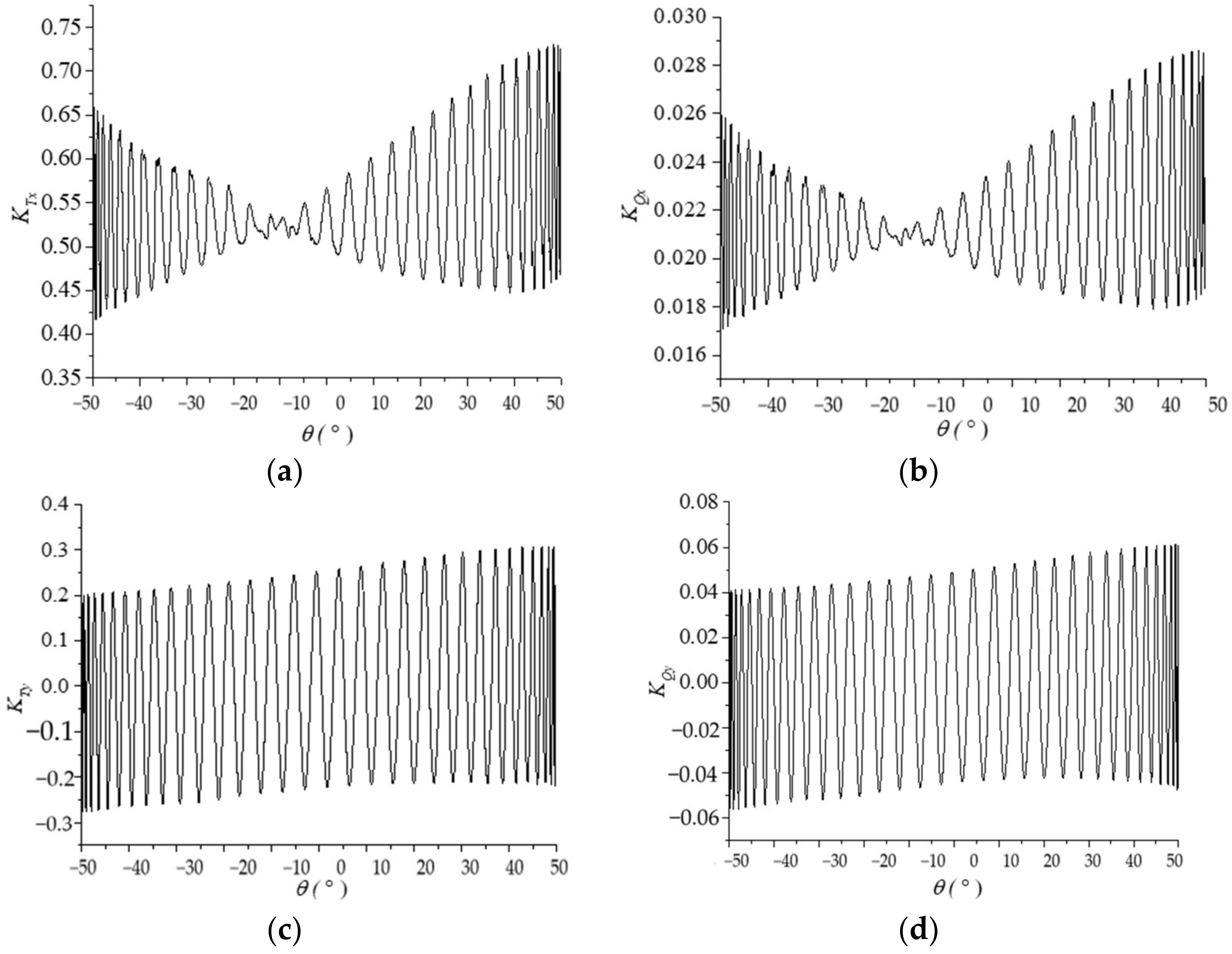
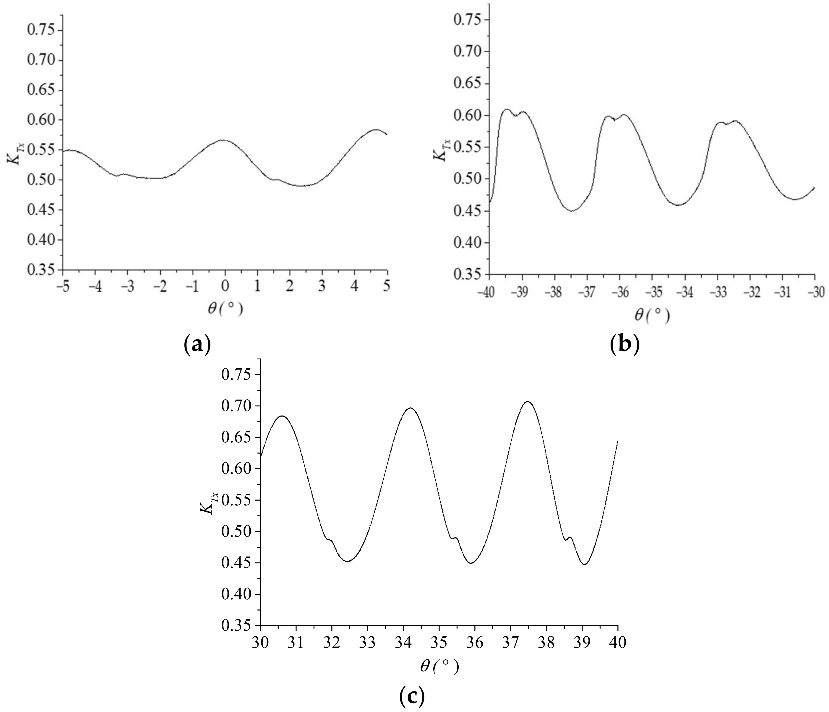
In fact, the hydrodynamic performance of the podded propeller will change under maneuvering conditions due to the influence of inflow velocity and swinging angle of the pod unit. For example, the thrust coefficients curve K_TPx and the torque coefficients curve K_QPx in the paddle X-direction will decrease as the advance number increases. During the swing process of the pod unit, the values of K_TPx and K_QPx will increase with the increase in the swing angle. It is interesting that under operating conditions, the disturbance effect of the pod unit on the flow field results in a greater load on the blade surface when the propeller is at a positive oblique flow angle. Therefore, we can see that when the pod unit swings to a positive angle, the value of K_TPx and K_QPx is significantly greater than the symmetrical negative angle. For K_TPy, under direct flow conditions, the value of the pod unit is 0.011 when rotating from starboard to port and −0.014 when rotating from port to starboard, with a difference of 21.4%. The value of K_QPz is −0.003 when the pod unit rotates from starboard to positive, and the value is 0.0045 when it rotates from positive to starboard under maneuvering conditions, with a difference of 50%. On the other hand, the value of K_QPz is 0 under steady-state conditions.

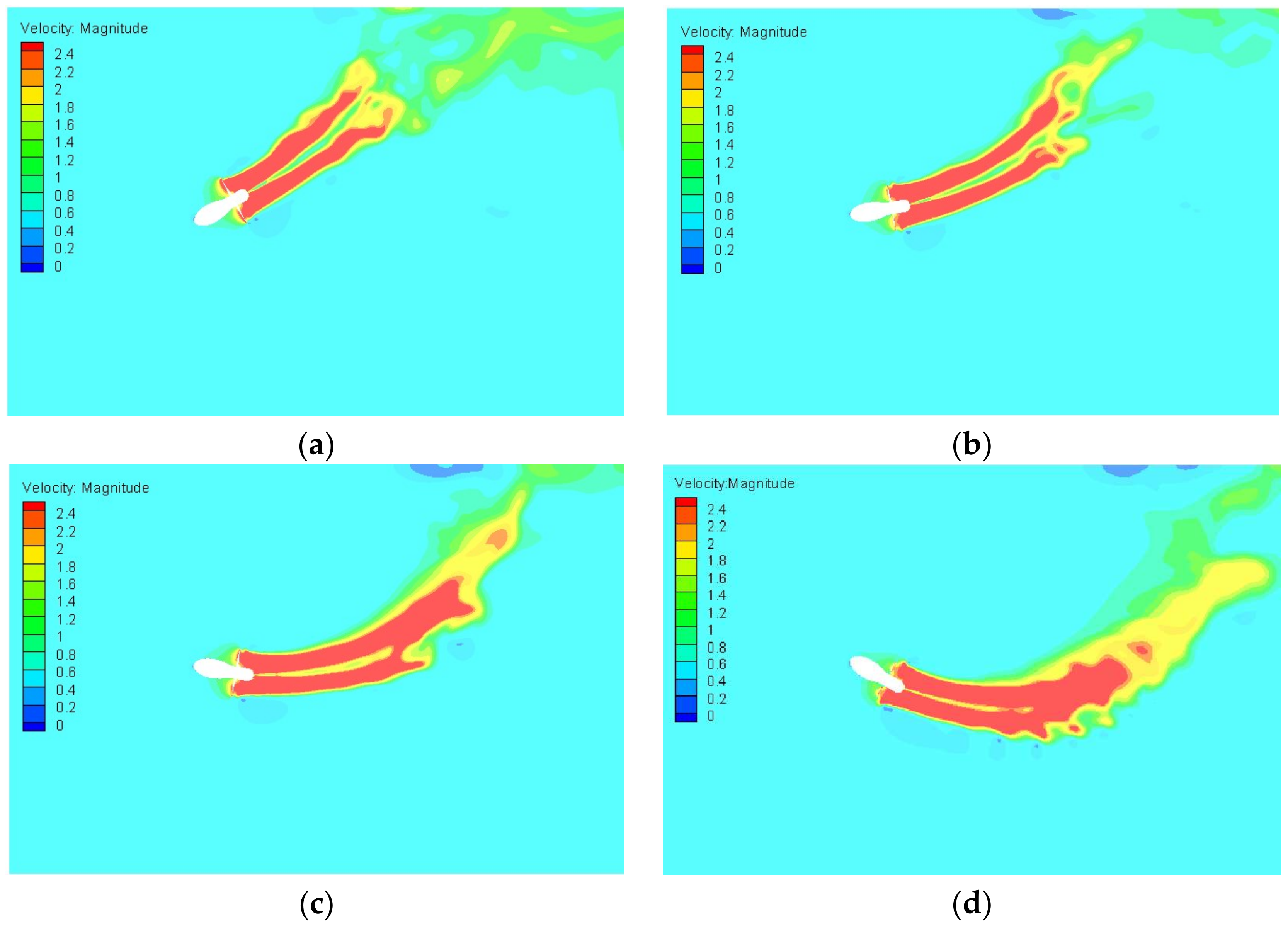
The single-blade load of the propeller is related to the diagonal flow angles. Under steady-state conditions, the value of K_Tx curve peak is positively correlated with the diagonal flow angles. Under maneuvering conditions, the wave amplitude is positively correlated with the diagonal flow angles, and the mean and peak values at the positive oblique flow angle are larger than those at the symmetrical negative oblique flow angle. The wake flow field of the propeller is curved owing to the rotational effect of the pod unit under the maneuvering conditions. This study provides a reference for the subsequent design of podded propellers and for the optimization ships’ shape.

The next step of the work will be to conduct experimental research on the hydrodynamic characteristics of the podded propeller under maneuvering conditions.

References

1. Bal, Ş.; Güner, M. Performance analysis of podded propulsors. Ocean. Eng. 2009, 36, 556–563. [Google Scholar] [CrossRef]
2. Wang, Z.Z.; Xiong, Y.; Wang, R.; Zhong, C.H. Numerical investigation of the scale effect of hydrodynamic performance of the hybrid CRP pod propulsion system. Appl. Ocean. Res. 2016, 54, 26–38. [Google Scholar] [CrossRef]
3. Sánchez-Caja, A.; Pylkkänen, J. Optimization of podded propulsor for fast ropax using RANS solver with cavitation model. In Proceedings of the International Conference on Fast Sea Transportation, Saint-Petersburg, Russia, 27–30 June 2005. [Google Scholar]
4. Xiong, Y.; Ye, J. Prediction of podded propulsion hydrodynamic performance by surface-panel method. J. Nav. Univ. Eng. 2007, 19, 41–45. [Google Scholar]
5. Zhao, D.; Guo, C.; Su, Y.; Dou, P.; Jing, T. Experimental study on hydrodynamics of L-type podded propulsor in straight-ahead motion and off-design conditions. J. Mar. Sci. Appl. 2017, 16, 48–59. [Google Scholar] [CrossRef]
6. Islam, M.F.; Veitch, B.; Liu, P. Experimental research on marine podded propulsors. J. Nav. Archit. Mar. Eng. 2008, 4, A276. [Google Scholar] [CrossRef]
7. Cao, M.; Wang, G.; Zhu, M. Experimental investigations on the hydrodynamic performance of podded propulsors. J.-Shanghai Jiaotong Univ. 2003, 37, 1198–1200. (In Chinese) [Google Scholar]
8. Shamsi, R.; Ghassemi, H. Numerical simulation of turbulent flow around podded propeller in azimuthing conditions. In Proceedings of the International Conference on Offshore Mechanics and Arctic Engineering, Glasgow, Scotland, 9–14 November 2012; American Society of Mechanical Engineers: New York, NY, USA, 2012; pp. 241–248. [Google Scholar]
9. Xie, Q.; Yi, X.; Wang, G.; Qian, X. Experimental Investigation on Hydrodynamic of Azinuthing Podded Propulsor. Ship Build. China 2008, 49, 6. [Google Scholar]
10. Xu, J.; Xiong, Y.; Wang, Z. Numerical research of hydrodynamic performance of hybrid CRP podded propulsor in steering conditions. Chin. J. Ship Res. 2017, 12, 63–70, 99. [Google Scholar]
11. Liu, P.; Islam, M.; Veitch, B. Unsteady hydromechanics of a steering podded propeller unit. Ocean. Eng. 2009, 36, 1003–1014. [Google Scholar] [CrossRef]
12. Shen, X.; Fan, S.; Cai, Y.; Sun, Q.; Yang, C. Experimental investigation on cavitation performance of podded propulsor under small helm-angle condition. Shipbuild 2012, 53, 1–8. [Google Scholar]
13. Reichel, M. Manoeuvring forces on azimuthing podded propulsor model. Pol. Marit. Res. 2007, 14, 3–8. [Google Scholar] [CrossRef]
14. El Moctar, O.; Junglewitz, A.; Lloyd, G. Numerical Analysis of the Steering Capability of a Podded Drive. Ship Technol. Res. 2004, 51, 134–145. [Google Scholar] [CrossRef]
15. Stettler, J.W.; Hover, F.S.; Triantafyllou, M.S. Preliminary Result of Testing on the Dynamics of an Azimuthing Podded Propulsor Relating to the Vehicle in Podded Propulsion; University of New Castle: Tyne, UK, 2004; pp. 321–338. [Google Scholar]
16. Islam, M.F.; Akinturk, A.; Veitch, B.; Liu, P. Performance characteristics of static and dynamic azimuthing podded propulsor. In Proceedings of the First International Symposium on Marine Propulsors–SMP’09, Trondheim, Norway, 22–24 June 2009; pp. 482–492. [Google Scholar]
17. Amini, H.; Steen, S. Theoretical and experimental investigation of propeller shaft loads in transient conditions. Int. Shipbuild. Prog. 2012, 59, 55–82. [Google Scholar]
18. Islam, M.; Akinturk, A.; Veitch, B. Performance Aspects of Podded Propulsor in Dynamic Operating Conditions. Int. Shipbuild. Prog. 2015, 62, 139–160. [Google Scholar] [CrossRef]
19. Akinturk, A.; Islam, M.F.; Veitch, B.; Liu, P. Performance of dynamic azimuthing podded propulsor. Int. Shipbuild. Prog. 2012, 59, 83–106. [Google Scholar]
20. Xingrong, S.; Xuemei, F.; Rongquan, C.; Yuejin, C. Study on hydrodynamic performance of podded propulsion in viscous flow. In Proceedings of the First International Symposium on Marine Propulsors—SMP, Trondheim, Norway, 22–24 June 2009; p. 9. [Google Scholar]
21. Islam, M.; Jahra, F.; Ryan, R.; Hedd, L. Hydrodynamics of Podded Propulsors With Highly Loaded Propellers and in Extreme Azimuthing Conditions. In Proceedings of the ASME 2015 34th International Conference on Ocean, Offshore and Arctic Engineering, St. John, NL, Canada, 31 May–5 June 2015; American Society of Mechanical Engineers Digital Collection: Houston, TX, USA, 2015. [Google Scholar]
22. Zhao, W.; Hu, J.; Chen, C.G. Numerical Simulation on the Hydrodynamic Performance of Azimuthing Podded Propulsors. In Proceedings of the 30th International Ocean and Polar Engineering Conference, Virtual, 11 October 2020; International Society of Offshore and Polar Engineers: Mountain View, CA, USA, 2020. [Google Scholar]
23. Mewis, F. The efficiency of pod propulsion. In Proceedings of the HADMAR, 22nd International Conference, Varna, Bulgaria, 1–4 October 2001. [Google Scholar]
24. Ortolani, F.; Dubbioso, G. Experimental investigation of blade and propeller loads: Steady turning motion. Appl. Ocean. Res. 2019, 91, 101874. [Google Scholar] [CrossRef]
25. Ortolani, F.; Capone, A.; Dubbioso, G.; Alves Pereira, F.; Maiocchi, A.; Di Felice, F. Propeller performance on a model ship in straight and steady drift motions from single blade loads and flow field measurements. Ocean. Eng. 2020, 197, 106881. [Google Scholar] [CrossRef]
26. Ortolani, F.; Dubbioso, G.; Muscari, R.; Mauro, S.; Di Mascio, A. Experimental and numerical investigation of propeller loads in off-design conditions. J. Mar. Sci. Eng. 2018, 6, 45. [Google Scholar] [CrossRef]
27. Reichel, M. Application of the IMO standard manoeuvres procedure for pod-driven ships. J. Mar. Sci. Technol. 2020, 25, 249–257. [Google Scholar] [CrossRef]
28. Reichel, M. Equivalent standard manoeuvres for pod-driven ships. Ocean. Eng. 2019, 187, 106165. [Google Scholar] [CrossRef]
29. Reichel, M. Prediction of manoeuvring abilities of 10000 DWT pod-driven coastal tanker. Ocean. Eng. 2017, 136, 201–208. [Google Scholar] [CrossRef]
30. Guo, H.; Guo, C.; Hu, J.; Lin, J.; Zhong, X. Influence of jet flow on the hydrodynamic and noise performance of propeller. Phys. Fluids 2021, 33, 065123. [Google Scholar] [CrossRef]
31. Hu, J.; Yan, Q.; Ding, J.; Sun, S. Numerical study on transient four-quadrant hydrodynamic performance of cycloidal propellers. Eng. Appl. Comput. Fluid Mech. 2022, 16, 1813–1832. [Google Scholar] [CrossRef]
Figure 1. Geometric parameters of the pod and strut (mm).
Jmse 11 00874 g001
Figure 2. 3D view of the pod unit.
Jmse 11 00874 g002
Figure 3. Computational domain.
Jmse 11 00874 g003
Figure 4. Regional definition of the model: (a) Full rotation domain (b) cylindrical rotation domain.
Jmse 11 00874 g004
Figure 5. Uptown view of the pod unit in oblique flow: (a) Maneuvering condition (b) Steady condition.
Jmse 11 00874 g005
Figure 6. Schematic of forces acting on the pod unit.
Jmse 11 00874 g006
Figure 7. Surface grid: (a) Pod unit surface grid (b) Blade surface grid.
Jmse 11 00874 g007
Figure 8. Fluid domain grid: (a) XZ plane (b) XY plane (c) YZ plane.
Jmse 11 00874 g008
Figure 9. Pressure distribution on the propeller surface: (a) Medium Grid (b) Fine Grid.
Jmse 11 00874 g009
Figure 10. Hydrodynamic performance comparison curve between the experiment and numerical simulation of the podded propeller.
Jmse 11 00874 g010
Figure 11. Comparison of podded propeller hydrodynamic performance: (a) Thrust coefficients (b) Torque coefficients.
Jmse 11 00874 g011
Figure 12. Comparison of propeller loads in each direction at different advanced coefficients: (a) KTPx; (b) KQPx; (c) KTPy; (d) KQPy; (e) KTPz; (f) KQPz.
Jmse 11 00874 g012
Figure 13. Comparison between steady load and the transient load of the propeller (J = 0.2): (a) KTPx; (b) KQPx; (c) KTPy; (d) KQPy; (e) KTPz; (f) KQPz.
Jmse 11 00874 g013aJmse 11 00874 g013b
Figure 14. Single-blade load in stable condition (J = 0.2): (a) KTx; (b) KTy; (c) KTz.
Jmse 11 00874 g014
Figure 15. Load of the single blade under maneuvering conditions (J = 0.2): (a) KTPx; (b) KQPx; (c) KTPy; (d) KQPy.
Jmse 11 00874 g015
Figure 16. Partial image of Figure 14a: (a) −5° to 5°; (b) −40° to −30°; (c) 30° to 40°.
Jmse 11 00874 g016
Figure 17. Process of changing the pod unit from starboard to port under maneuvering conditions (J = 0.2): (a) Oblique flow −30°; (b) Oblique flow −10°; (c) Oblique flow 10°; (d) Oblique flow 30°.
Jmse 11 00874 g017
Figure 18. Flowline on blade surface (J = 0.2).
Jmse 11 00874 g018
Figure 19. Streamline at tip of paddle.
Jmse 11 00874 g019
Figure 20. r/R = 0.7 cross-section streamline.
Jmse 11 00874 g020
Figure 21. Velocity X in the transverse section (J = 0.2): (a) x/D = 1.6 maneuvering condition; (b) x/D = 3.2 maneuvering condition; (c) x/D = 1.6 steady-state conditions; (d) x/D = 3.2 steady-state conditions.
Jmse 11 00874 g021