
A Numerical Study on the Performance of the 66k DWT Bulk Carrier in Regular and Irregular Waves
 , , and
Abstract
:1. Introduction
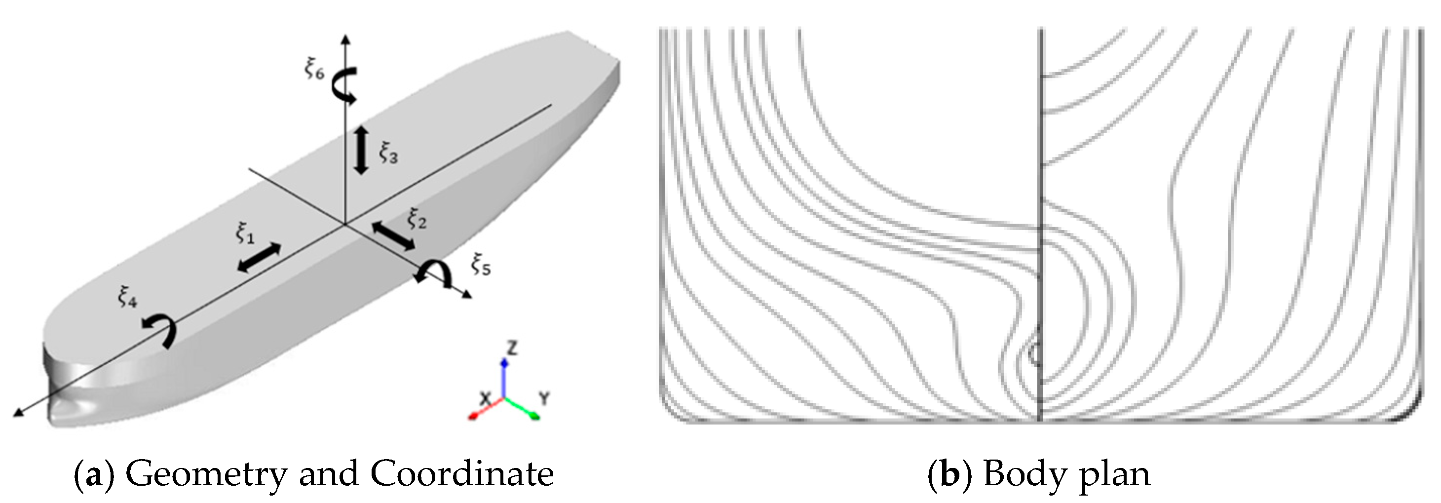
2. Objective Ship
3. Numerical Method and Condition
3.1. Numerical Set-Up
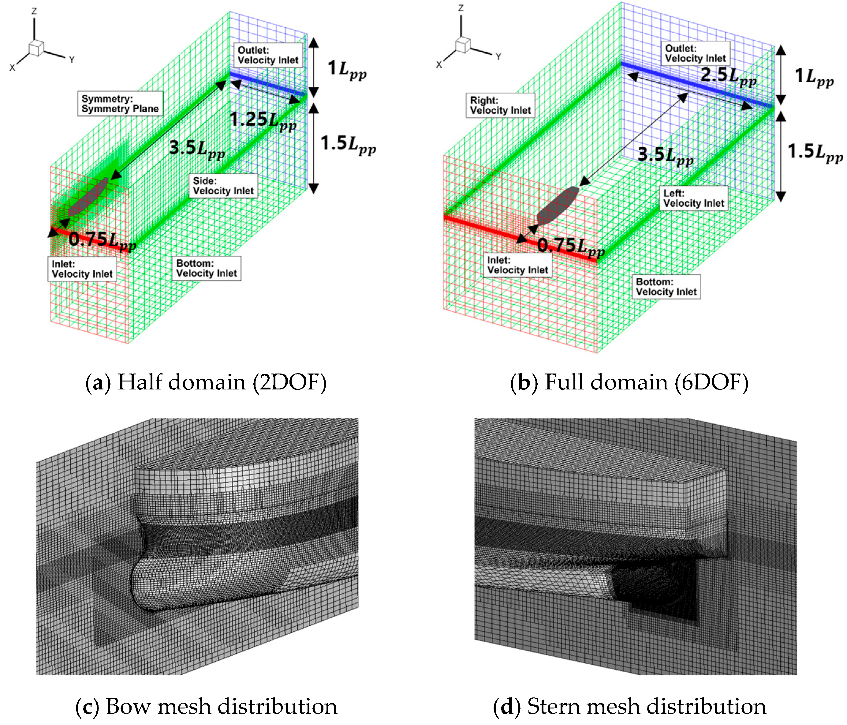
3.2. Grid System and Boundary Condition
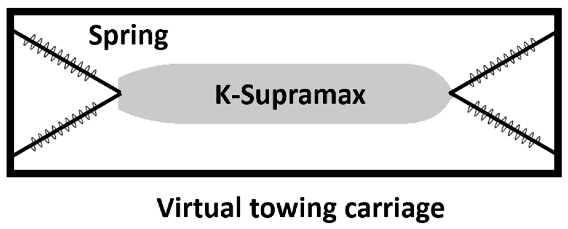
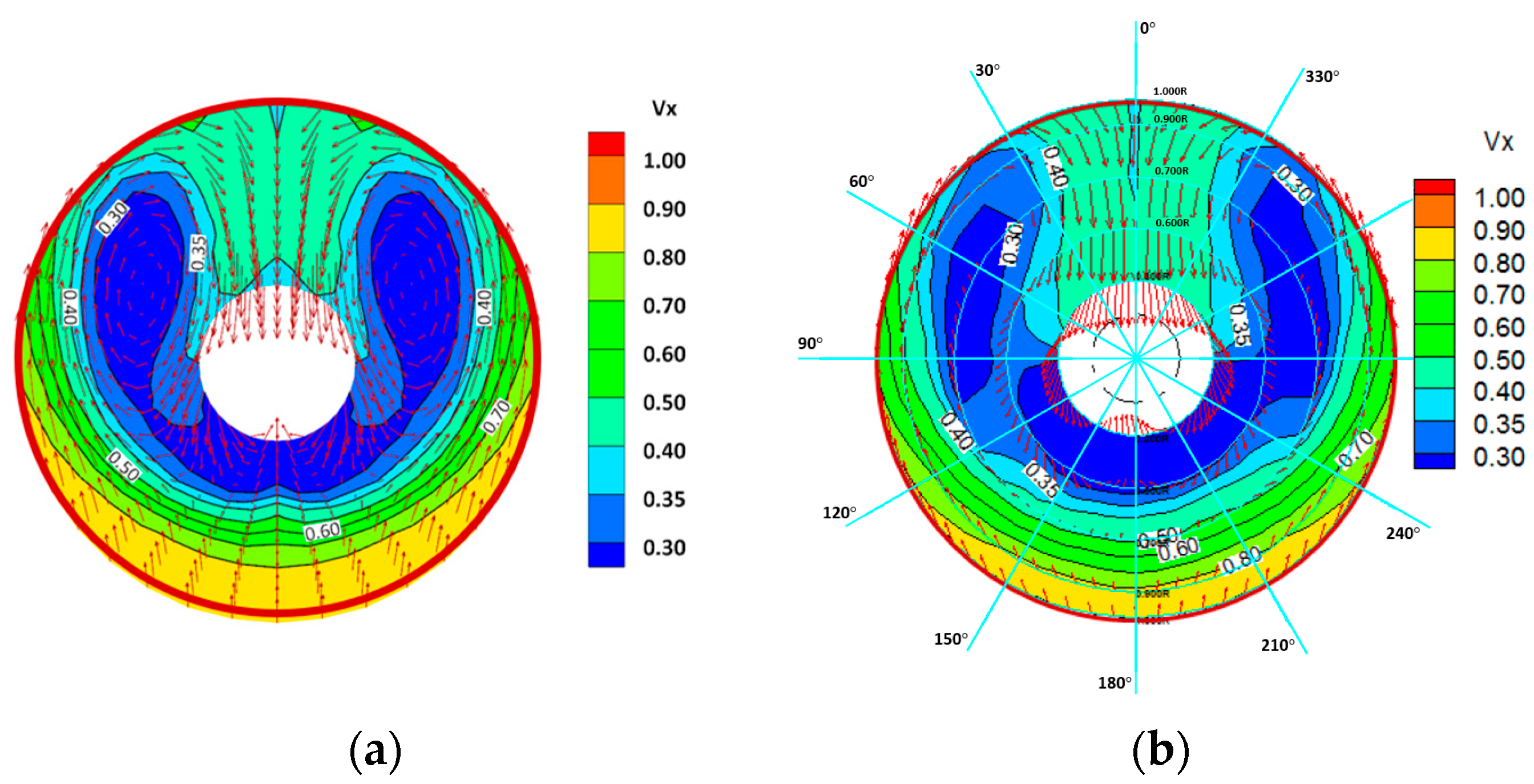
3.3. DOF Simulation Method
4. Validation and Verification
4.1. Free Decay Test
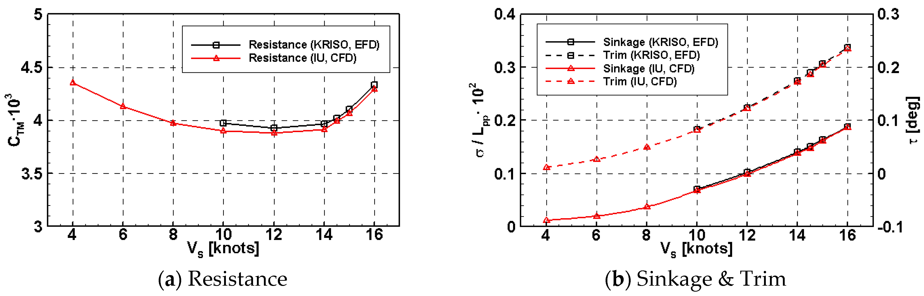
4.2. Calm Water Simulation
5. Regular Wave
5.1. Regular Wave Simulation Condition
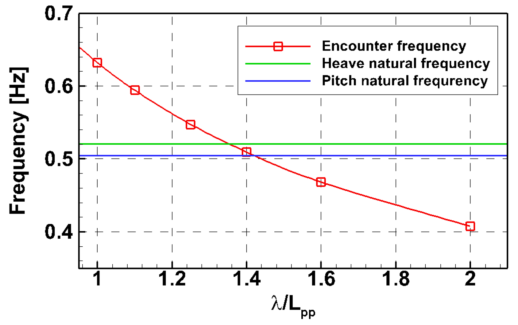
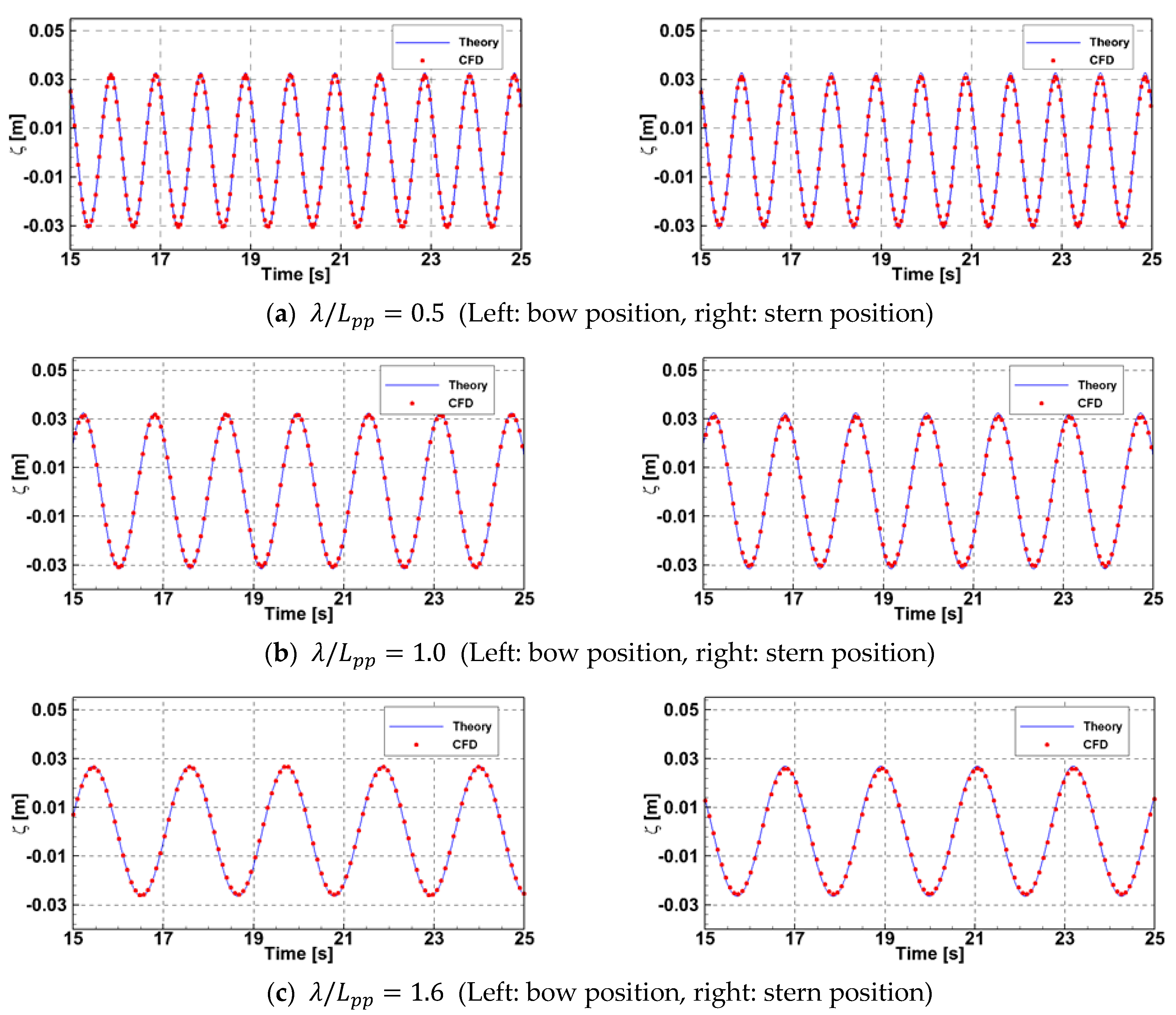
5.2. Regular Wave Test
5.3. Convergence Grid Test in Regular Wave
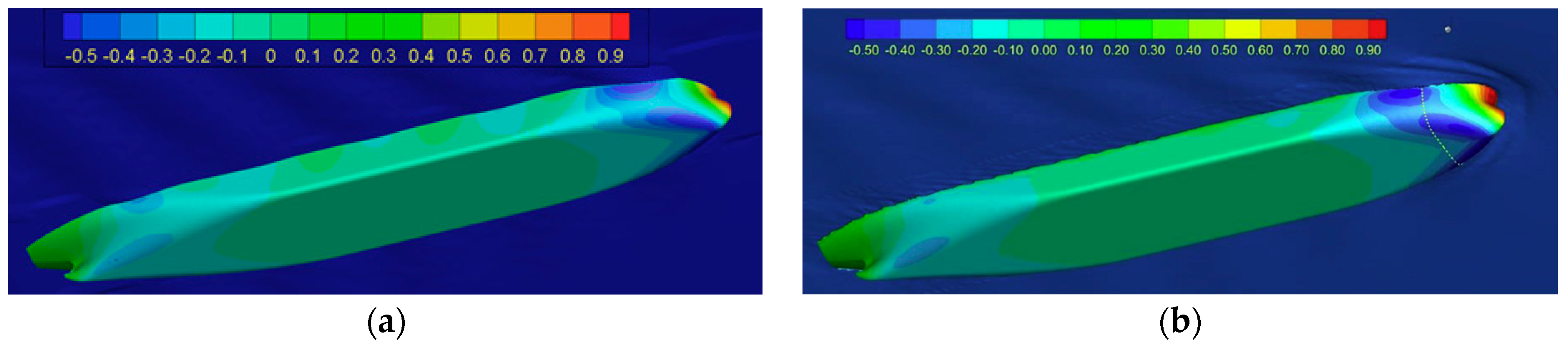
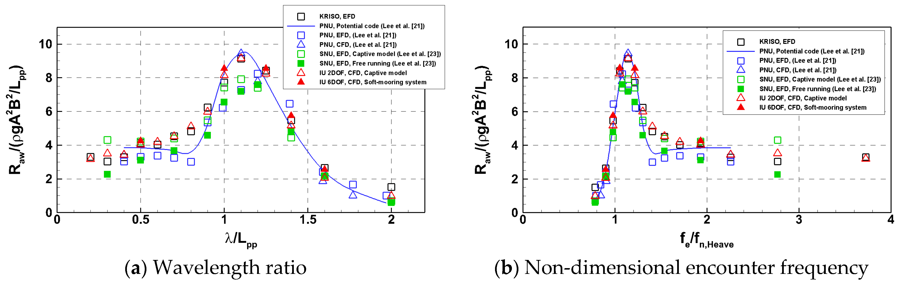
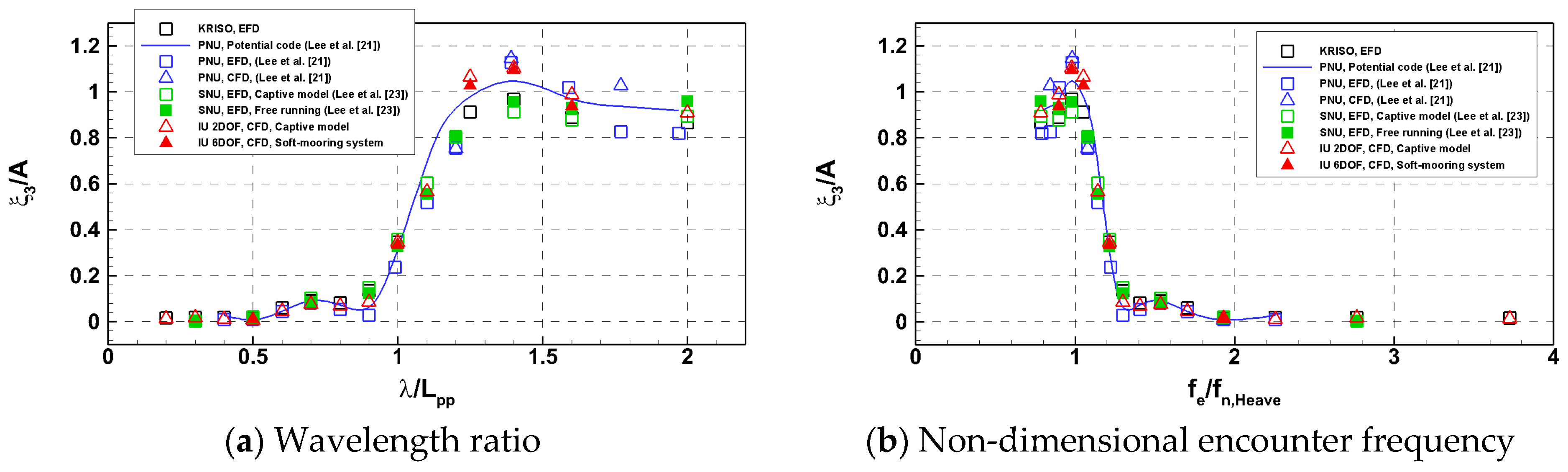
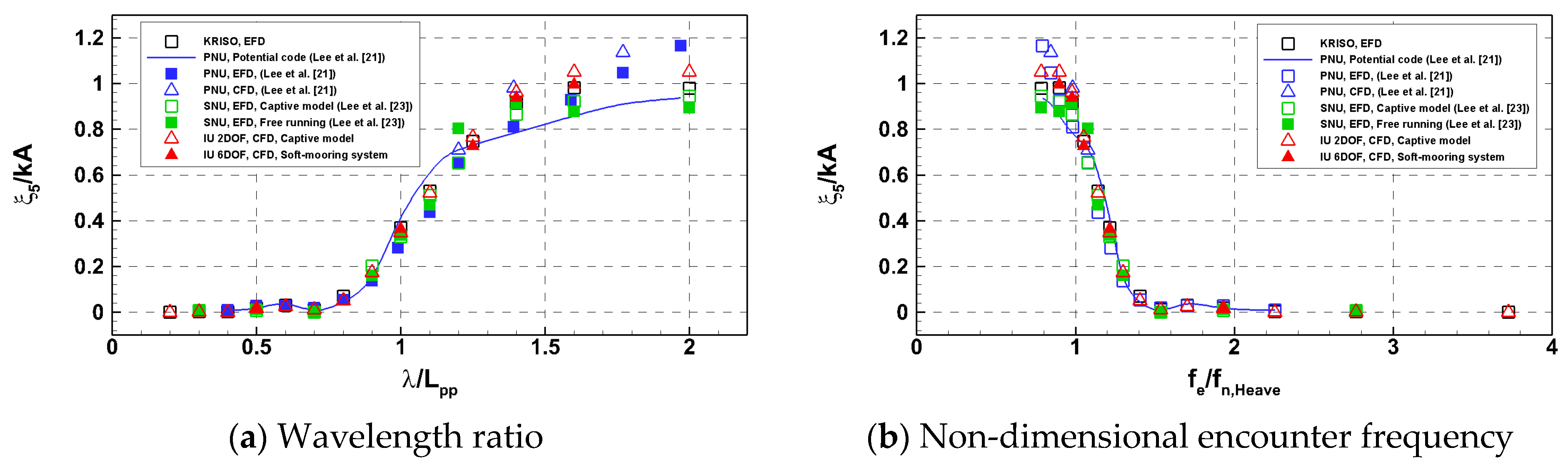
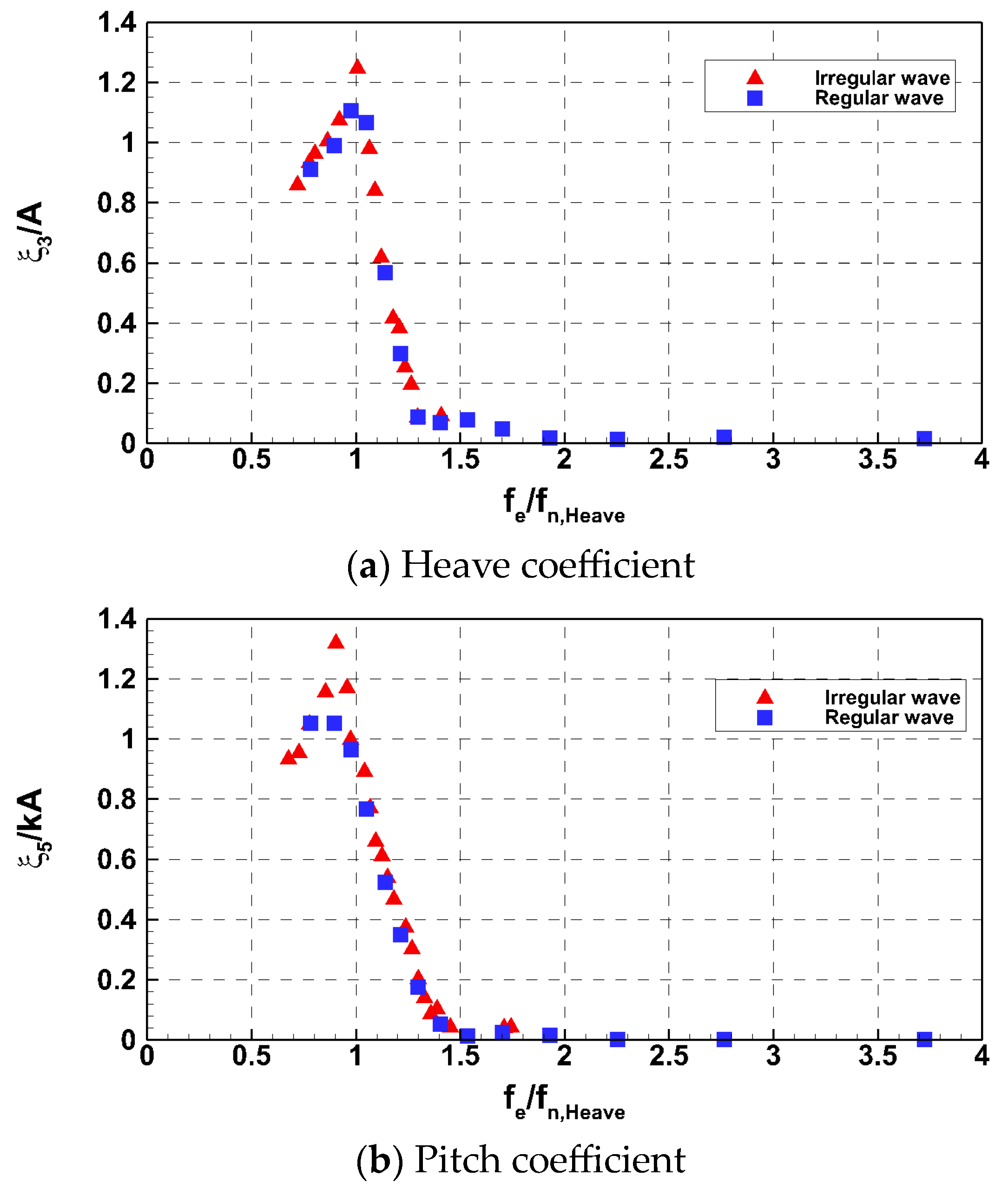
5.4. Resistance Performance in a Regular Wave
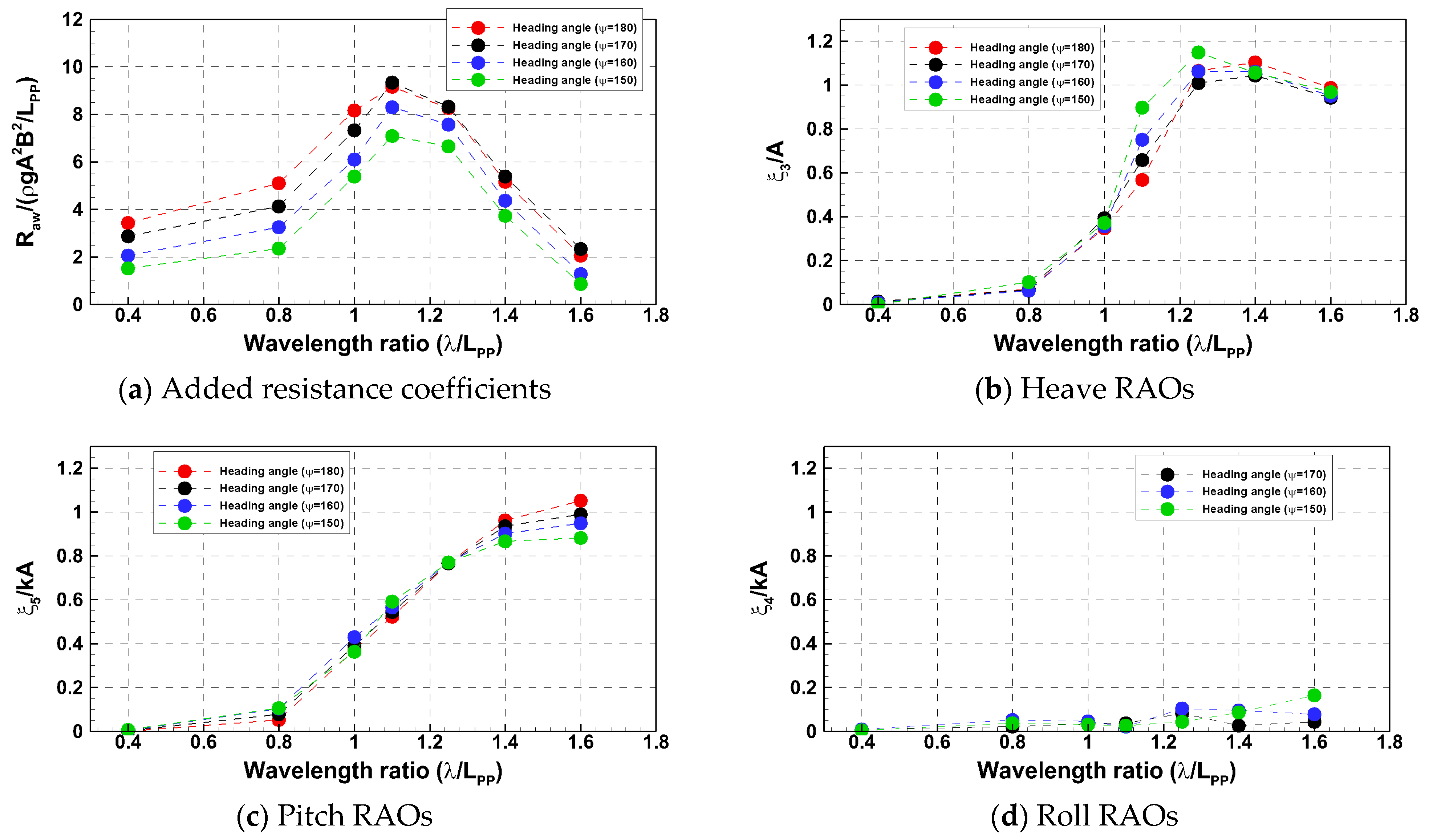
5.5. Resistance Performance in the Regular Wave with Various Heading Angles
6. Irregular Wave
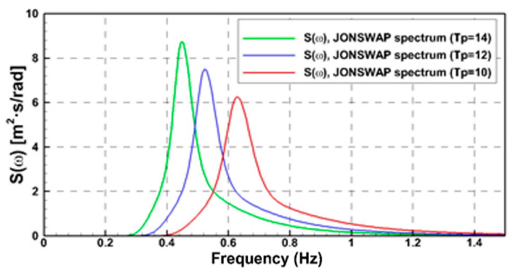
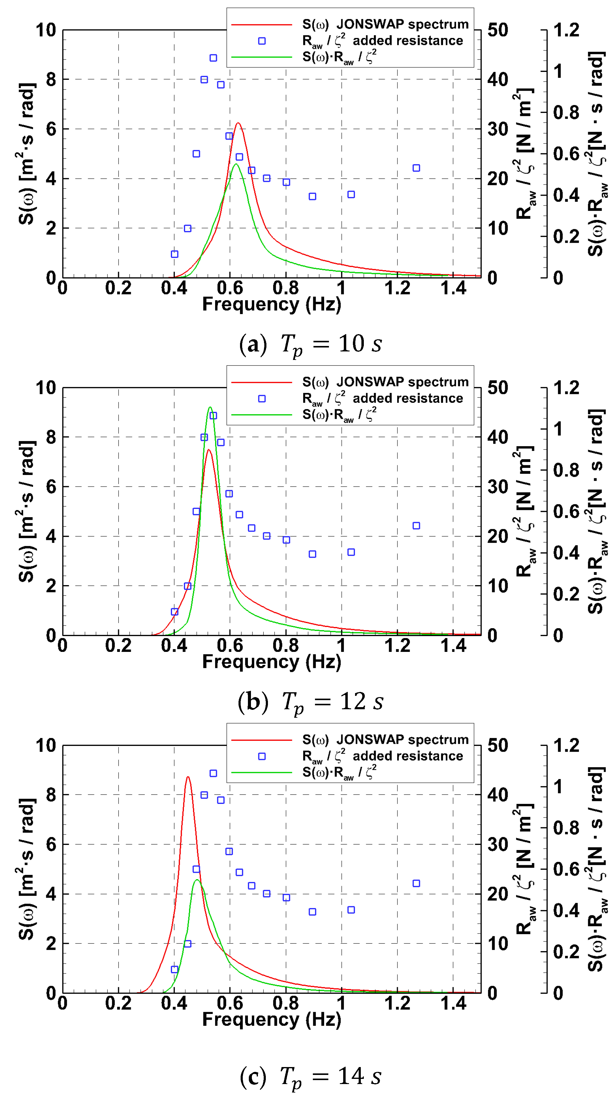
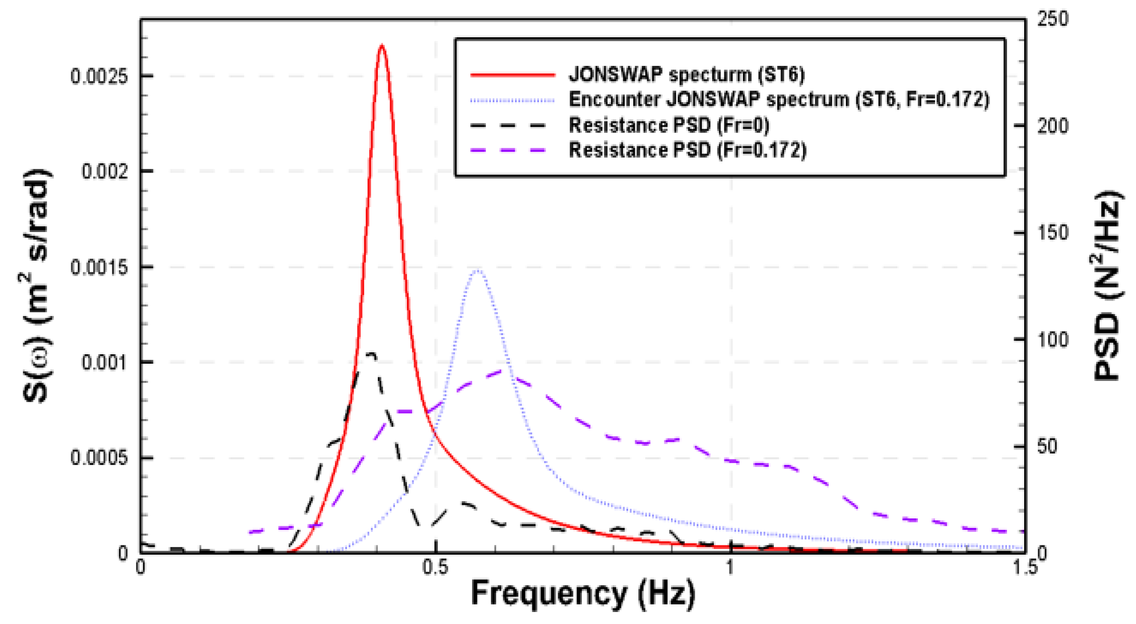
6.1. Resistance Performance in Irregular Waves Using the Spectral Method (Indirect Method)
6.2. Resistance Performance in an Irregular Wave through Direct Computation
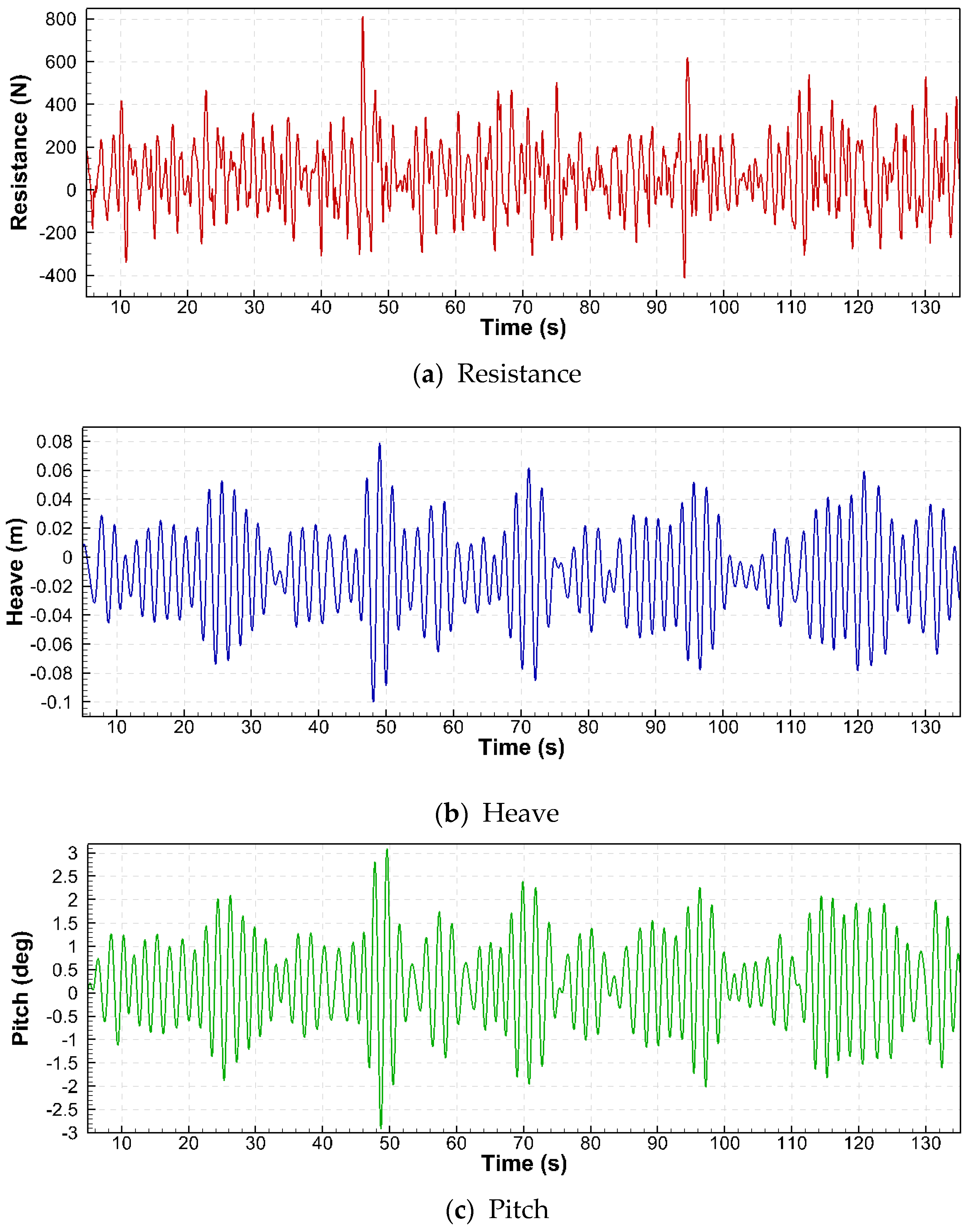
6.3. Resistance Performance in an Irregular Wave Using CFD Simulation
7. Conclusions
Author Contributions
Funding
Institutional Review Board Statement
Informed Consent Statement
Conflicts of Interest
References
- MEPC.1/Circ.850/Rev.3. Progress of the 2013 Interim Guidelines for Determining Minimum Propulsion Power to Maintain the Manoeuvrability of Ships in Adverse Conditions. J. Soc. Nav. Archit. Korea 2021, 56, 497–506. [Google Scholar]
- Prpić-Oršić, J.; Faltinsen, O.M. Estimation of Ship Speed Loss and Associated CO2 Emissions in a Seaway. Ocean Eng. 2012, 44, 1–10. [Google Scholar] [CrossRef]
- St. Denis, M.; Pierson, W.J. On the Motions of Ships in Confused Seas. Trans. Soc. Nav. Archit. Mar. Eng. 1953, 61, 280–357. [Google Scholar]
- Lewis, E.V.; Bennet, R. Lecture Notes on Ship Motions in Irregular Seas; Webb Institute of Naval Architecture: Glen Cove, NY, USA, 1963. [Google Scholar]
- Gerritsma, J.; van den Bosch, J.J.; Beukelman, W. Propulsion in Regular and Irregular Waves. Int. Shipbuild. Prog. 1961, 8, 235–247. [Google Scholar] [CrossRef]
- Ström-Tejsen, J. Added Resistance in Waves. Soc. Nav. Archit. Mar. Eng. 1973, 81, 250–279. [Google Scholar]
- Fujii, H.; Takahashi, T. Experimental Study on the Resistance Increase of a Large Full Ship in Regular Oblique Waves. J. Soc. Nav. Archit. Jpn. 1975, 1975, 132–137. [Google Scholar] [CrossRef]
- Journee, J.M.J. Experiments and Calculations on 4 Wigley Hull Forms in Head Sea. Delft Univ. Technol. Rep. 1992, 909. [Google Scholar]
- Guo, B.J.; Steen, S. Evaluation of Added Resistance of Kvlcc2 in Short Waves. J. Hydrodyn. 2011, 23, 709–722. [Google Scholar] [CrossRef]
- Hwang, S.; Ahn, H.; Lee, Y.Y.; Kim, M.S.; Van, S.H.; Kim, K.S.; Van, S.H.; Jang, Y.H. Experimental Study on the Bow Hull-Form Modification for Added Resistance Reduction in Waves of KVLCC2. In Proceedings of the 26th International Ocean and Polar Engineering Conference, Rhodes, Greece, 26 June 2016. [Google Scholar]
- Lee, J.; Park, D.-M.; Kim, Y. Experimental Investigation on the Added Resistance of Modified KVLCC2 Hull Forms with Different Bow Shapes. J. Eng. Marit. Environ. 2017, 231. [Google Scholar] [CrossRef]
- Maruo, H.; Tokura, J. Prediction of Hydrodynamic Forces and Moments Acting on Ships in Heaving and Pitching Oscillations by Means of an Improvement of the Slender Ship Theory. J. Soc. Nav. Archit. Jpn. 1978, 1978, 104–112. [Google Scholar] [CrossRef]
- Gerritsma, J.; Beukelman, W. Analysis of the Resistance Increase in Waves of a Fast Cargo Ship. Int. Shipbuild. Prog. 1972, 19, 285–293. [Google Scholar] [CrossRef]
- Boese, P. Eine Einfache Methode Zur Berechnung Der Widerstandserhöhung Eines Schiffes Im Seegang. J. Schiffstechnik 1970, 17, 1–18. [Google Scholar]
- Sadat-Hosseini, H.; Wu, P.C.; Carrica, P.M.; Kim, H.; Toda, Y.; Stern, F. CFD Verification and Validation of Added Resistance and Motions of KVLCC2 with Fixed and Free Surge in Short and Long Head Waves. Ocean Eng. 2013, 59, 240–273. [Google Scholar] [CrossRef]
- Park, I.-R.; Kim, J.; Suh, S.-B.; Kim, J.; Kim, K.-S.; Kim, Y.-C. Numerical Prediction of the Powering Performance of a Car-Ferry in Irregular Waves for Safe Return to Port(SRtP). J. Ocean Eng. Technol. 2019, 33, 1–9. [Google Scholar] [CrossRef]
- Shin, H.W.; Paik, K.J.; Jang, Y.H.; Eom, M.J.; Lee, S. A Numerical Investigation on the Nominal Wake of KVLCC2 Model Ship in Regular Head Waves. Int. J. Nav. Archit. Ocean Eng. 2020, 12, 270–282. [Google Scholar] [CrossRef]
- Eom, M.J.; Paik, K.J.; Jang, Y.H.; Ha, J.Y.; Park, D.W. A Method for Predicting Propeller Performance Considering Ship Motion in Regular Waves. Ocean Eng. 2021, 232, 109135. [Google Scholar] [CrossRef]
- Lee, S.H.; Paik, K.J.; Hwang, H.S.; Eom, M.J.; Kim, S.H. A Study on Ship Performance in Waves Using a RANS Solver, Part 1: Comparison of Power Prediction Methods in Regular Waves. Ocean Eng. 2021, 227, 108900. [Google Scholar] [CrossRef]
- Lee, S.H.; Paik, K.J.; Cho, J.H.; Kim, G.H.; Kim, H.S.; Kim, S.H. A Numerical Study on Self-Propulsion Performance in Regular Waves and Power Prediction in Irregular Waves. Int. J. Nav. Archit. Ocean Eng. 2022, 14, 100454. [Google Scholar] [CrossRef]
- Lee, C.M.; Park, S.C.; Yu, J.W.; Choi, J.E.; Lee, I. Effects of Diffraction in Regular Head Waves on Added Resistance and Wake Using CFD. Int. J. Nav. Archit. Ocean Eng. 2019, 11, 736–749. [Google Scholar] [CrossRef]
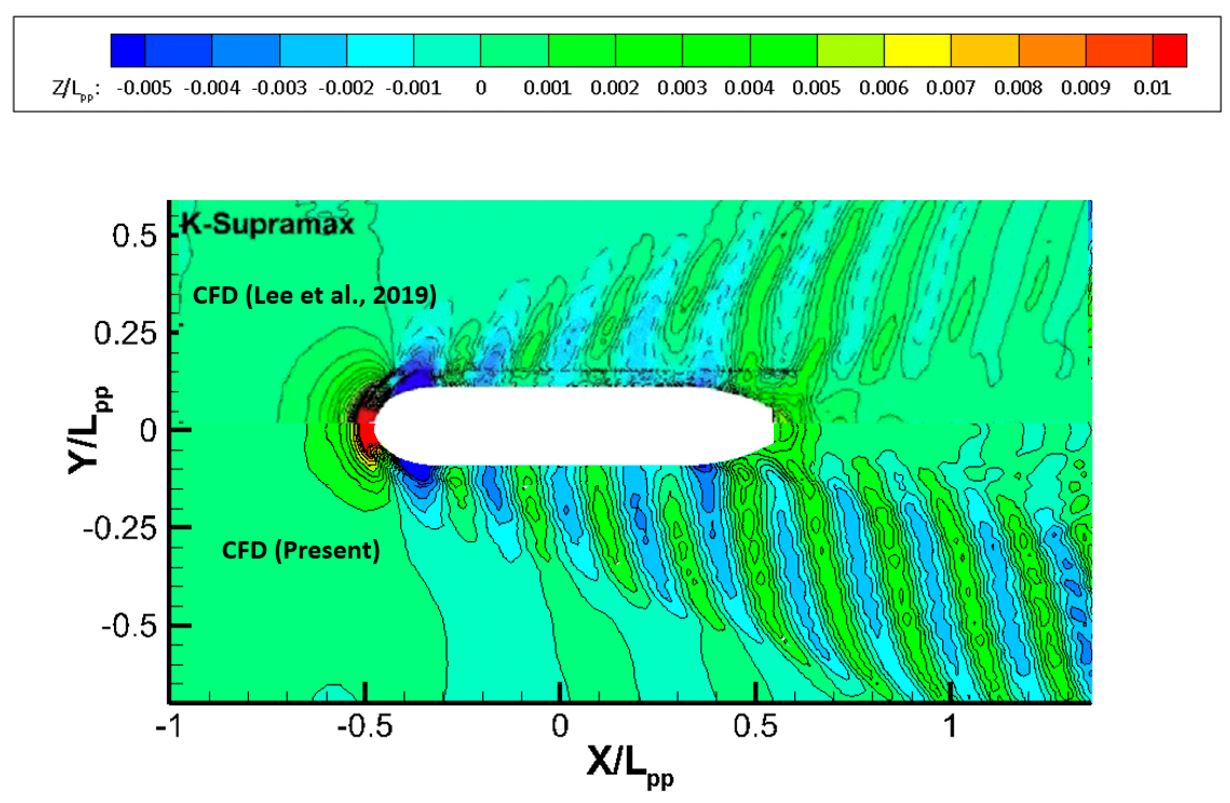
- Lee, C.M.; Yu, J.W.; Choi, J.E.; Lee, I. Effect of Bow Hull Forms on the Resistance Performance in Calm Water and Waves for 66k DWT Bulk Carrier. Int. J. Nav. Archit. Ocean Eng. 2019, 11, 723–735. [Google Scholar] [CrossRef]
- Lee, J.H.; Kim, Y.; Kim, B.S.; Gerhardt, F. Comparative Study on Analysis Methods for Added Resistance of Four Ships in Head and Oblique Waves. Ocean Eng. 2021, 236, 109552. [Google Scholar] [CrossRef]
- Cho, J.H.; Lee, S.H.; Oh, D.; Paik, K.J. A Numerical Study on the Added Resistance and Motion of a Ship in Bow Quartering Waves Using a Soft Spring System. Ocean Eng. 2023, 280, 114620. [Google Scholar] [CrossRef]
- Shih, T.-H.; Liou, W.W.; Shabbir, A.; Yang, Z.; Zhu, J. A New K-Epsilon Eddy Viscosity Model for High Reynolds Number Turbulent Flows. Comput. Fluid 1994, 24, 227–238. [Google Scholar] [CrossRef]
- Lewis, E.V. Principles of Naval Architecture, Vol. III: Motions in Waves and Controllability; The Society of Naval Architects and Marine Engineers: Jersey City, NJ, USA, 1989. [Google Scholar]
- Jang, J.; Choi, S.H.; Ahn, S.M.; Kim, B.; Seo, J.S. Experimental Investigation of Frictional Resistance Reduction with Air Layer on the Hull Bottom of a Ship. Int. J. Nav. Archit. Ocean Eng. 2014, 6, 363–379. [Google Scholar] [CrossRef]
- Celik, I.B.; Ghia, U.; Roache, P.J.; Freitas, C.J.; Coleman, H.; Raad, P.E. Procedure for Estimation and Reporting of Uncertainty Due to Discretization in CFD Applications. J. Fluids Eng. Trans. ASME 2008, 130, 0780011–0780014. [Google Scholar] [CrossRef]
- Lee, S.H.; Paik, K.J.; Lee, J.H. A Study on Ship Performance in Waves Using a RANS Solver, Part 2: Comparison of Added Resistance Performance in Various Regular and Irregular Waves. Ocean Eng. 2022, 263, 112174. [Google Scholar] [CrossRef]
- ISO 15016:2015; Ships and Marine Technology—Guidelines for the Assessment of Speed and Power Performance by Analysis of Speed Trial Data. International Organization for Standardization: Geneva, Switzerland, 2015. Available online: https://www.iso.org/obp/ui/en/#iso:std:iso:15016:ed-2:v1:en (accessed on 20 September 2023).
- Maruo, H. The Excess Resistance of a Ship in Rough Seas. Int. Shipbuild. Prog. 1957, 4, 337–345. [Google Scholar] [CrossRef]


| Full-Scale | IU & KRISO | PNU [21] | SNU [23] | |
|---|---|---|---|---|
| Scale ratio, | 1 | 24 | 33.33 | 60, 40.42 |
| Length between perpendiculars, | 192 | 8 | 5.76 | 3.20, 4.75 |
| Length on waterline, | 196 | 8.16 | 5.88 | 3.27, 4.85 |
| Breadth, | 36 | 1.50 | 1.08 | 0.60, 0.89 |
| Draft, | 11.2 | 0.47 | 0.34 | 0.19, 0.28 |
| Wetted surface area, | 9808 | 17.03 | 8.83 | 2.72, 6.00 |
| Displacement, | 65,028 | 4.70 | 1.76 | 0.30, 0.98 |
| Block coefficient, | 0.8400 | |||
| Midship section coefficient, | 0.9973 | |||
| Free Motion | |
|---|---|
| ① Heave ② Heave, Pitch ③ Surge, Sway, Heave, Roll, Pitch, Yaw | |
| ① Pitch ② Heave, Pitch ③ Surge, Sway, Heave, Roll, Pitch, Yaw |
| Empirical Formula | 1DOF | 2DOF | 6DOF | ||||
|---|---|---|---|---|---|---|---|
| Free condition | Heave | Pitch | Heave Pitch | Heave Pitch | All | All | |
| Initial condition | |||||||
| 0.5438 | 0.5540 | 0.5208 | 0.5222 | 0.5236 | 0.5270 | ||
| 0.5660 | 0.5475 | 0.5042 | 0.5051 | 0.5123 | 0.5097 | ||
| Wave Steepness | 2DOF | 6DOF |
|---|---|---|
| Case No. | Number of Grids | GCI (%) | |||
|---|---|---|---|---|---|
| Grid | G1T2 | 2,169,732 | 350 | 8.686 | 0.515 |
| G2T2 | 3,687,345 | 350 | 8.149 | ||
| G3T2 | 7,514,440 | 350 | 8.030 | ||
| Timestep | G2T1 | 3,687,345 | 150 | 8.823 | 0.242 |
| G2T2 | 3,687,345 | 350 | 8.149 | ||
| G2T3 | 3,687,345 | 700 | 8.015 |
| Less than | 4.5 | 7.0 to 15.0 | 19.0 |
| Parameters linearly interpolated, depending on the ship length | |||
| More than | 6.0 | 7.0 to 15.0 | 22.6 |
| Peak Wave Period | Total Resistance |
|---|---|
| 10 | 138.69 |
| 12 | 151.43 |
| 14 | 127.24 |
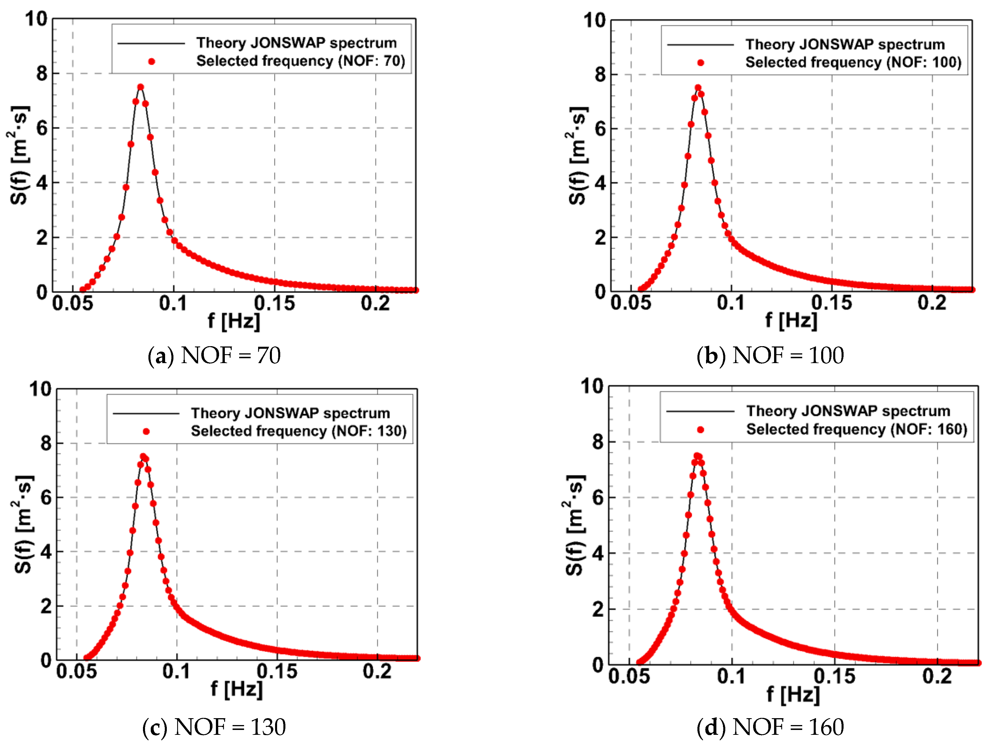
| Frequency Number | Wave Period (s) |
|---|---|
| 70 | 85.36 |
| 100 | 122.47 |
| 130 | 159.59 |
| 160 | 196.70 |
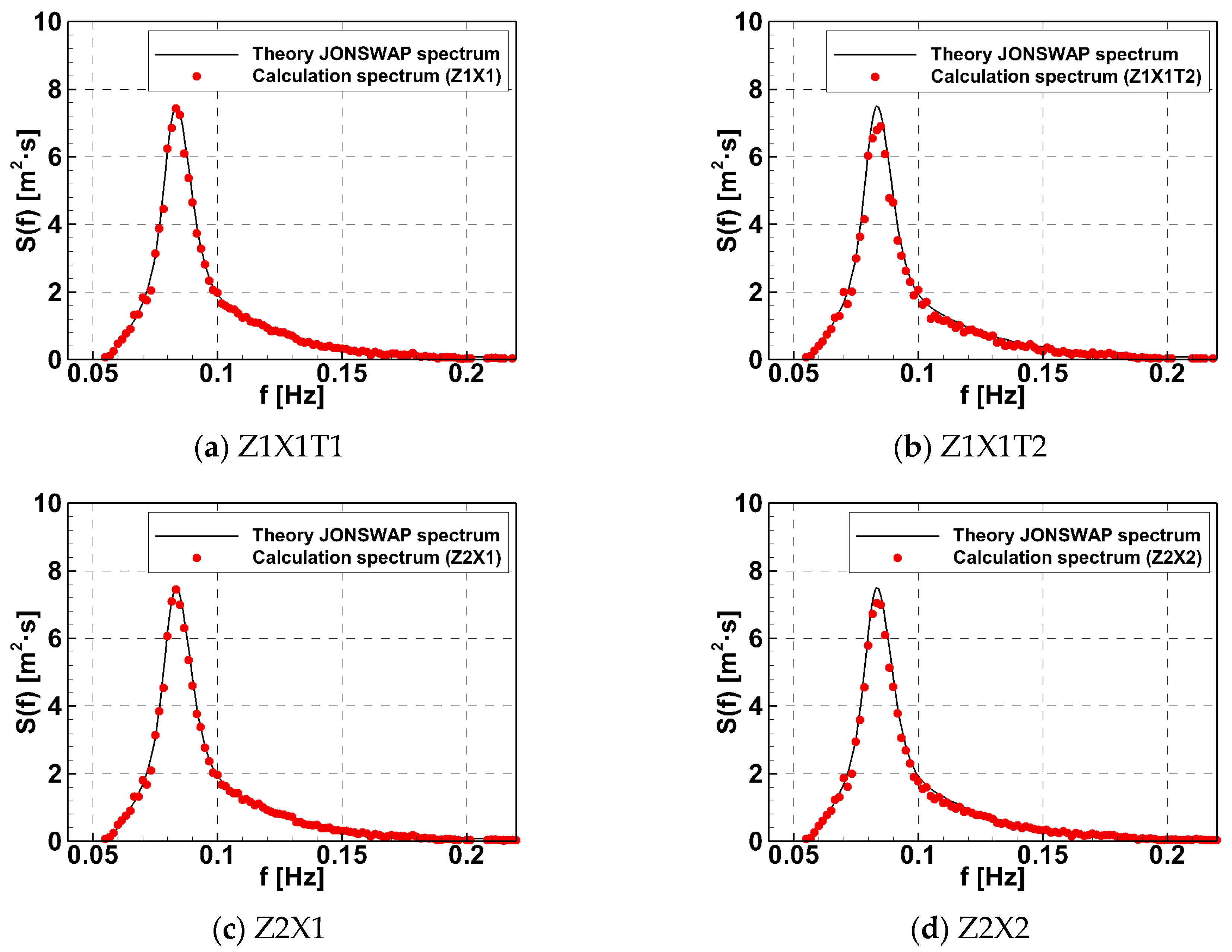
| Z1X1 | Z1X1T2 | Z2X1 | Z2X2 | |
|---|---|---|---|---|
| 876 | 438 | 876 | 876 | |
| 64 | 64 | 64 | 32 | |
| 80 | 80 | 160 | 160 |
| Condition | Total Resistance [N] | |
|---|---|---|
| Calm water, | 78.68 | - |
| Spectral method (Indirect method), | 154.43 | 1.96 |
| Direct computation (Direct method), | 134.98 | 1.71 |
Disclaimer/Publisher’s Note: The statements, opinions and data contained in all publications are solely those of the individual author(s) and contributor(s) and not of MDPI and/or the editor(s). MDPI and/or the editor(s) disclaim responsibility for any injury to people or property resulting from any ideas, methods, instructions or products referred to in the content. |
© 2023 by the authors. Licensee MDPI, Basel, Switzerland. This article is an open access article distributed under the terms and conditions of the Creative Commons Attribution (CC BY) license (https://creativecommons.org/licenses/by/4.0/).
Share and Cite
Kim, G.-H.; Hwang, S.; Lee, S.-H.; Lee, J.-H.; Hwangbo, J.; Kim, K.-S.; Paik, K.-J. A Numerical Study on the Performance of the 66k DWT Bulk Carrier in Regular and Irregular Waves. J. Mar. Sci. Eng. 2023, 11, 1913. https://doi.org/10.3390/jmse11101913
Kim G-H, Hwang S, Lee S-H, Lee J-H, Hwangbo J, Kim K-S, Paik K-J. A Numerical Study on the Performance of the 66k DWT Bulk Carrier in Regular and Irregular Waves. Journal of Marine Science and Engineering. 2023; 11(10):1913. https://doi.org/10.3390/jmse11101913
Chicago/Turabian StyleKim, Gu-Hyeon, Seunghyun Hwang, Soon-Hyun Lee, Jun-Hee Lee, Jun Hwangbo, Kwang-Soo Kim, and Kwang-Jun Paik. 2023. "A Numerical Study on the Performance of the 66k DWT Bulk Carrier in Regular and Irregular Waves" Journal of Marine Science and Engineering 11, no. 10: 1913. https://doi.org/10.3390/jmse11101913