Optimal Design of Flow Control Fins for a Small Container Ship Based on Machine Learning

Abstract

In this study, the optimal design of flow control fins (FCFs) for a container ship was carried out via a machine learning approach. The conventional design practice for the FCF relied on simulation-based performance evaluation, which demands a large amount of analysis time. Instead of computational fluid dynamics (CFD)-based prediction, artificial neural network (ANN)-based prediction was attempted. Prior to the machine learning process, the wake distribution data were collected systematically via CFD. Based on the collected data, the wake distributions and resistance performance dependent on varying the fin positions were learned using the ANN, and the optimal fin position was selected with relevant optimization techniques. When multi-objective optimization was employed, it was found that both wake distributions and resistance performance were improved in a practically applicable timeframe. The current process is superior to conventional simulation-based optimization in terms of speed. From the viewpoint of prediction accuracy, in this study, ANN-based prediction was found to be equally accurate as CFD-based prediction. Thus, the results can provide a novel and reliable design methodology for the optimal design of ship appendages.

1. Introduction

1.1. Importance of Flow Control Fins (FCFs) in Ship Energy Efficiency

In response to the Paris Agreement of 2015, the International Maritime Organization (IMO) adopted an initial strategy for reducing greenhouse gas (GHG) emissions by ships in April 2018 [1]. The goal is to reduce total annual GHG emissions by 50% by 2050 compared to 2008, as well as to decrease carbon intensity (CI) by 40% by 2030 and by 70% by 2050, to decarbonize the shipping industry as soon as possible within this century. Various follow-up actions and programs to achieve the Initial Strategy are being undertaken. The Energy Efficiency eXisting ship Index (EEXI) and the Carbon Intensity Index (CII) came into effect as of 1 January 2023 (IMO 2021). These are significant reinforcements of the energy-saving regulations for existing ships. Therefore, retrofitting an energy saving device (ESD) on existing ships is drawing significant attention among ship operators and shipbuilders.

Among various ESDs, flow control fins (FCFs), alternatively known by the commercial brand name SAVER (SAmsung Vibration and Energy Reduction) Fin, attached to the stern are noted as an appropriate option for retrofitting. This device has a few notable advantages, such as its small size and simple rectangular shape, which result in low construction costs and a short payback period lasting less than a year. In addition, the fin is also reliable and safe even when structural failure occurs, since it is fitted far away from the propeller [2]. The two major roles of a FCF can be summarized as follows. Firstly, it can reduce viscous resistance through deflecting bilge vortices generated via changes in the hull cross-section area near the stern region, which slow down the upper part of the propeller inflow. Secondly, the FCF is one of the most efficient ways to homogenize the wake field distribution of already designed hull forms. The flow being hindered by bilge vortices prevents the pressure recovery of the hull surface in the stern part, thereby augmenting non-uniformity in propeller inflow distribution. This non-uniformity in the propeller wake acts as the main source of hull vibration due to uneven propeller loading.

Lee et al. [2] reported that a combination of the SAVER Fin and a rudder bulb led to a 7.4% power saving effect and 50% reduction in vibration for a 35k DWT bulk carrier, which was superior to the effect of a Mewis duct. Inoue and Saito [3] investigated the combination of fins separately set around the stern of a tanker hull with the aim of finding a target wake pattern at the propeller plane. Their Multi-ALV Fin was found to contribute to the reduction in the axial velocity on the propeller plane, resulting in an improvement in hull efficiency. It was found that the Multi-ALV Fin demonstrated an energy-saving effect of around 1% by itself. Recently, an optimization study by Park et al. [4] showed that the FCF leads to a 4.3% reduction in the total resistance of a 6.5k DWT tanker. Furthermore, the wake distribution was significantly improved due to the FCFs.

As shown in Figure 1, the conventional design process for a FCF is generally performed referring to a series of case studies with computational fluid dynamics (CFD) simulations. Depending on the experience of the designer, this process could involve many trials, and CFD analysis could take a considerable amount of time to perform. To reduce the time required for CFD analysis, a few studies were conducted that predicted wake distribution using various machine learning methodologies. Hwangbo and Shin [5] predicted wake distribution with a neural network using back-propagation from hull form information. Kim and Moon [6] predicted wake distribution using a neuro-fuzzy technique. Furthermore, Wie and Kim [7] applied a genetic algorithm and non-linear programming via quadratic Lagrangian (NLPQL) to design the optimal flow control fin.

Furthermore, in the hull-from design progress, optimization is attempted using a surrogate model. Pache and Rung [8] compared the performance of data-driven surrogate models, proper orthogonal decomposition (POD) and convolutional neural network-based autoencoder (CNN-AE) to predict aerodynamic pressure fields and forces on the superstructure of the container ship. Regarding the shape optimization of AUVs, Sun et al. [9] proposed a bionic hull shape (BHS) using a surrogate model and response surface methods (RSM). Zhang et al. [10] used a deep belt network (DBN) to reduce wave-making resistance by finding the optimal hull parameters of a Wigley ship.

In addition to hull-form design, machine learning is applied in various fields of the shipbuilding industry. Alexiou et al. [11] compared the performance of multiple regression algorithms, such as artificial neural network (ANN), tree regressions (TRs), random forest regression (RFR), k-nearest neighbor (kNN), linear regression and adaptive boosting (AdaBoost), in predicting the output power of the main engines (M/E) of an ocean-going vessel. Lin et al. [12], based on deep reinforcement learning (DRL), developed an efficient anti-rolling controller using a deep deterministic policy gradient (DDPG) algorithm.

1.2. Contributions

The purpose of this study is to select the optimal fin position to improve propeller inflow property and resistance performance. Here, the improved propeller inflow is associated with a small nominal wake fraction ($w_N$) and homogeneous wake distribution. The study was conducted based on two strategies: machine learning based on a neural network and optimization techniques. The neural network was used as a predictor of wake distribution for a given design variable of FCF. Thus, this study is an extension of Hwangbo and Shin’s [5] efforts to enable the design application of FCF. Regarding the optimization of FCF design variables, the sequential least squares programming (SLSQP) and the non-dominated sorting genetic algorithm II (NSGA-II) algorithms were employed for single- and multi-objective optimization problems, respectively. A combination of the prediction of wake distributions via machine learning with an appropriate optimization algorithm gives rise to an efficient, automatic optimization process in which time-consuming CFD simulation can be avoided. Furthermore, training results via neural networks can be transferred to design cases involving different hull forms. To the best of our knowledge, the present study is the first application of the machine learning technique to the optimal design of the FCF.

The paper’s organization is as follows: Section 2 describes the theoretical background of the artificial neural network (ANN) and the optimization algorithms used in this study; Section 3 formulates a numerical procedure to build the data sets; Section 4 explains the ANN-based prediction of wake distribution for the given design variables of FCFs and subsequent single- and multi-objective optimization processes; Section 5 presents the optimization results of FCF; and Section 6 discusses this study’s main conclusions and findings.

2. Theoretical Backgrounds

This section describes the theoretical backgrounds for the two major methodologies used in this study. (1) the feed-forward neural network used to predict the wake flow distribution for a given combination of design variables for FCF instead of CFD simulation; and (2) two algorithms, one for a single objective and the other for multiple objectives, used to optimize design variables for FCF.

2.1. Artificial Neural Network (ANN)

An artificial neural network is a computing system inspired by biological neural networks comprising animal brains [13]. This network was applied to solve problems such as regression analysis, classification and data processing. A feed-forward neural network, which converts input variable sets to output variable sets, can be regarded as a non-linear mathematical function. An accurate form of conversion is managed using a set of weights, which is determined through a process known as training [14]. In this study, multilayer perception (MLP), which is widely used in most practical applications of ANNs, was employed. Figure 2 illustrates a simplified expression of two-layer MLP. In this MLP, the hidden layer $z_j$ and the output layer $y_k$ are defined as follows:

$$z_j=g\left({\displaystyle \sum }_{i=0}^d{w}_{ji}{x}_i\right)$$

(1)

$$y_k=\tilde{g}\left({\displaystyle \sum }_{j=0}^m{\tilde{w}}_{ki}{z}_j\right), y_k=\tilde{g}\left({\displaystyle \sum }_{j=0}^m{\tilde{w}}_{ki}g\left({\displaystyle \sum }_{i=0}^d{w}_{ji}{x}_i\right)\right)$$

(2)

All layers of the ANN are independent of each other and consist of varying numbers of nodes. The nodes in the hidden layer are connected via the nodes in the preceding layer through weighted summation. The connected input is modified by the activation function, which can be embodied using mathematical functions, such as sigmoid, hyperbolic tangent and rectified linear unit (ReLU).

2.2. Optimization Algorithms

2.2.1. Sequential Least Squares Programming (SLSQP)

SLSQP minimizes a function of several variables with any combination of bounds, equality, and inequality constraints. The method wraps the SLSQP optimization subroutine originally implemented by Kraft [15]. Based on the iterative formulation and solution of quadratic programming subproblems, this method obtains subproblems using a quadratic approximation of the Lagrange function of a problem and via linearizing the constraints. The quadratic programming problem is then solved to obtain the search direction vector. SLSQP has advantages over linear search in terms of fast convergence and more accurate minimization. However, the existence of a minimum value is secured only if the objective function and constraint are concave [16]. Thus, SLSQP is ideal for mathematical problems for which the objective function and the constraints are twice continuously differentiable.

An SLSQP algorithm can solve the following bounded minimization problem.

$$\left\{ \begin{array}{l}Minimize f\left(x\right)\hfill \\ subject to g_j\left(x\right)=0, j\in E\hfill \\ g_u\left(x\right)\ge 0, u\in I\hfill \\ x_{iL}\le x_i\le x_{iU}, i=1,\dots ,n\hfill \end{array}\right.$$

(3)

Here, $f\left(x\right)$stands for the target scalar function to be minimized, with $x$ being the design parameter. $g_j\left(x\right)$ and $g_u\left(x\right)$ are equality and inequality constraints, respectively. $E$ and $I$ are the function set corresponding to the respective constraint type. Finally, $x_{iL}$ and $x_{iU}$ represent the lower and upper bounds of $x_i$, respectively.

After solving the quadratic programming subproblem to obtain the search direction vector $d$, the minimization vector $x^{\mathcal{l}+1}$ at $\left(\mathcal{l}+1\right)$-th step is iteratively updated using the following equation:

$$x^{\mathcal{l}+1}=x^{\mathcal{l}}+a^{\mathcal{l}}{d}^{\mathcal{l}}$$

(4)

Here, $d^{\mathcal{l}}$ and $a^{\mathcal{l}}$ represent the search direction and the iteration length at the $\mathcal{l}$-th iteration step.

2.2.2. Non-Dominated Sorting Genetic Algorithm-II (NSGA-II)

In general, it is not possible to obtain a single solution to minimize multiple objective functions simultaneously. The solution to multiple objective functions can only be sought in terms of a non-dominated solution, which is defined as the solution in which no one objective function can be improved without a simultaneous detriment to at least one of the other objectives [17]. The solution categorized as a non-dominated solution is also called a pareto-optimal solution, whose objective functions comprise a pareto-optimal front [18].

With a view to finding a pareto-optimal solution to the multiple objective optimization problem, the current study employed NSGA-II, which is one of the most representative genetic algorithms. The NSGA-II algorithm is an improved version of the NSGA algorithm [19], where the complexity of non-dominated sorting is diminished. The introduction of crowing distance led to a more efficient distribution of resources among individuals. Furthermore, the elitism was adopted to ensure the inheritance the optimal solution of the parent generation by the offspring generation [20].

Figure 3 presents a conceptual flow chart of NSGA-II. In the first step, the initial population is generated based on the objective functions and constraints, and the fitness function is then evaluated. After non-dominating sorting, the offspring population is generated through means of three fundamental operations of the genetic algorithm—selection, crossover and mutation. The parent and offspring population are combined, and the individuals for the new parent population are subsequently selected based on elitism and crowding distance. These steps are iterated until the stopping criteria is satisfied.

3. Problem Description

3.1. Geometry of Target Ship and Flow Control Fins

In this study, a 1000 TEU container ship built by Daesun Shipbuilding and Engineering Co. Ltd. was designated as the baseline hull form. This model was chosen due to the availability of a reliable CFD database with a high level of correlation with model test data. In addition, this vessel belongs to the feeder class of 1000~1999 TEU, which is the most frequently built container ship class. A model with a scale ratio of $\lambda =30.56$ was considered for both numerical simulations. The principal particulars of the baseline hull and propeller are listed in

Table 1. Principal particulars of 1000 TEU container ship.

Designation	Symbol (Unit)	Full-Scale Ship
Length bet. perpendiculars	$L_{PP}$ (m)	137.5
Breadth	$B$ (m)	23.6
Draft	$T$ (m)	7.4
Block coefficient	$C_B$	0.595
Propeller diameter	$D$ (m)	5.5

. Figure 4 illustrates 3D volumetric views of the baseline hull form and propeller.

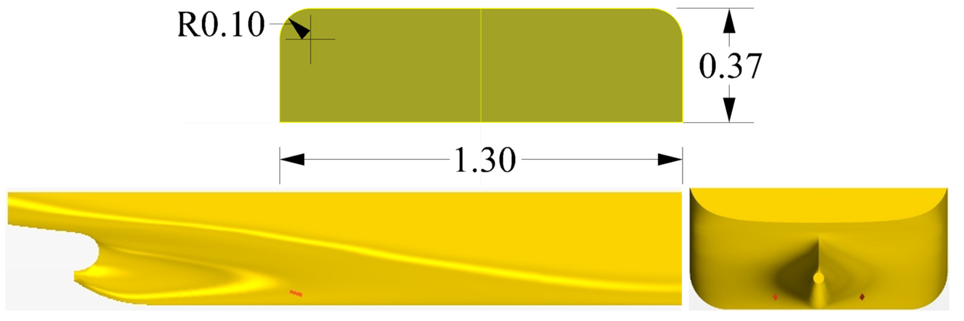
The flow control fins (FCFs) employed in this study were in the shape of a rectangular plate with rounded corners, as shown in Figure 5. The dimensions of the FCF were 1.30 m (length) × 0.37 m (height) × 0.03 m (thickness) in full scale. These dimensions correspond to $0.236 D$ (length) × $0.0673 D$ (height) × $0.00545 D$ (thickness) in terms of propeller diameter, $D$. As shown in Figure 5, the FCFs are attached perpendicularly to the hull surface on the stern part of the hull. Usually, the FCFs are attached in pair(s) at the same positions on the port and starboard sides. The design variables of the FCF adopted in this study were the longitudinal and vertical positions of the FCF and the inclination angle. Here, the position of the FCF corresponds to the midpoint of the baseline, and the inclination angle corresponds to the angle formed between the baseline of the FCF and the baseline of the hull. Depending on the design variables of the FCF, the downstream flow is affected differently in terms of spatial extent and velocity increment. In other words, the design variables of the FCF are optimized to change the propeller inflow in the intended manner, i.e., to be accelerated and become more uniform. The objective function for the optimization process will be described in detail in Section 4.2.

3.2. CFD Simulation for Training Data

In order to train, validate and test the neural network, a total of 693 data sets were obtained via the CFD analysis. Each data set corresponded to one design parameter set, with total design parameter sets being a combination of 11 longitudinal positions $\left(3.0\le x/St\le 4.0, \Delta x/St=0.1\right)\times 21$ vertical positions $\left(0.135\le z/T\le 0.405, \Delta z/T=0.0135\right)\times 3$ inclination angles $\left(\alpha =19°,20°,21°\right)$. Here, $St$ represents the station length, which is 1/20 of the length between perpendicular $L_{PP}$.

For the CFD analysis of the flow around a ship hull, the commercial CFD package STAR-CCM+ v.15.06 was employed. The governing equations for the CFD analysis are the continuity equation and Reynolds-Averaged Navier–Stokes (RANS) equation. These equations are expressed in tensor notation as follows:

$$\frac{\mathsf{\partial }{U}_i}{\mathsf{\partial }{x}_i}=0$$

(5)

$$\frac{\mathsf{\partial }{U}_i}{\mathsf{\partial }t}+\rho U_l\frac{\mathsf{\partial }{U}_i}{\mathsf{\partial }{x}_l}=-\frac{\mathsf{\partial }p}{\mathsf{\partial }{x}_i}+\frac{\mathsf{\partial }}{\mathsf{\partial }{x}_l}\left(\mu \frac{\mathsf{\partial }{U}_i}{\mathsf{\partial }{x}_l}-\rho \overline{u_i{u}_l}\right)+\rho g_i$$

(6)

where $U_i=\left(U,V,W\right)$ is the velocity component in the $x_i=\left(x,y,z\right)$ direction, while $p, \rho , \mu ,-\overline{u_i{u}_l}$ and $g_i$ are the static pressure, fluid density, fluid viscosity, Reynolds stress and gravitational acceleration in the $x_i$-direction, respectively.

The Reynolds stress turbulence model, which is known to be excellent in resolving bilge vortex and capable of high-accuracy prediction of the flow around a ship hull [21], was employed in the numerical analysis. The transport equation, derived from the RANS equation, is given as follows:

$$\frac{\mathsf{\partial }\overline{u_i^{\text{'}}{u}_j^{\text{'}}}}{\mathsf{\partial }t}=D_{ij}+G_{ij}-\frac{2}{3}{\delta }_{ij}\epsilon +PS$$

(7)

where ${\delta }_{ij}$ is the Kronecker delta and $D_{ij}$, $G_{ij}$ and $PS$ correspond to the diffusion, production and pressure strain terms, respectively, which are defined as follows:

$$D_{ij}=\frac{\mathsf{\partial }}{\mathsf{\partial }{x}_l}\left(C_k\frac{k^2}{\epsilon }\frac{\mathsf{\partial }\overline{u_i{u}_j}}{\mathsf{\partial }{x}_l}+\nu \frac{\mathsf{\partial }\overline{u_i{u}_j}}{\mathsf{\partial }{x}_l}\right)$$

(8)

$$G_{ij}=-\left(\overline{u_i{u}_l}\frac{\mathsf{\partial }{U}_j}{\mathsf{\partial }{x}_l}+\overline{u_j{u}_l}\frac{\mathsf{\partial }{U}_j}{\mathsf{\partial }{x}_l}\right)$$

(9)

$$PS=-C_1\frac{\epsilon }{k}\left(\overline{u_i{u}_j}-\frac{2}{3}{\delta }_{ij}k\right)-C_2\left(G_{ij}-\frac{2}{3}{\delta }_{ij}{G}_k\right)$$

(10)

Here, $C_k$, $C_1$ and $C_2$ are turbulent model constants. In addition, $k$ and $\epsilon$ stand for the turbulent kinetic energy and dissipation rate, respectively.

Figure 6 illustrates the computational domain, which is a rectangle occupying the range of $-2.5 L_{PP}<x<L_{PP}, 0<y<1.5 L_{PP}$ and $-1.5 L_{PP}<z<0$. Due to the symmetry about the centerplane $\left(y=0\right)$, only half of the domain was considered. Furthermore, double-body simulation, in which the underwater hull is mirrored about the free surface $\left(z=0\right)$, was carried out for all simulation cases. Through completing this step, wave generation due to the ship hull and consequent wave-making resistance was neglected. However, this process does not cause any complications in analyzing the effect of varying the FCF design on the flow field because the deep submergence of FCFs prevents them from affecting the free surface. Through omitting the time-consuming free surface calculations, the double-body simulation can significantly shorten the analysis time, which is crucial as this study involves numerous test cases. The boundary conditions for the surfaces of the computational domain in Figure 6 are summarized in

Table 2. Boundary conditions for Figure 6.

Boundary Surface	Type
Inlet	Velocity inlet
Outlet	Pressure outlet
Top, bottom, side, centerplane	Symmetry
Ship	Wall

.

It is worthwhile to mention that automation in pre-processing steps, such as geometry modeling and mesh generation, is of profound importance for the sake of overall computational efficiency for the entire 693 simulation cases. Processes such as 3D modeling of the hull form with varying FCF, mesh generation, and creation of CFD settings for each case were performed with professional hull form design S/W of OptHull^® (Cadas Co., Ltd., Changwon, Republic of Korea) The subsequent processes involved in the configuration of STAR-CCM+ and analysis automation were controlled via an in-house JavaScript code. Using a Message Passing Interface (MPI) parallel computing cluster consisting of 140 CPU cores (Intel Xeon 2.6 GHz), it took approximately 323 h to complete the 693 simulations required for the preparation of data.

4. Methodologies

4.1. ANN-Based Prediction of Wake Distribution

Before training the neural network, the flow field data obtained from the CFD analysis were pre-processed. A harmonic analysis was performed to find Fourier series coefficients for the axial velocity distribution in the form of a $73\times 8$ polar array, as shown in Figure 7. To be more specific, for eight radial positions in the range $0.3R<r<1.0R \left(\Delta r=0.1R\right)$, the circumferential distribution of axial velocity $V_x\left(\phi \right)$ was represented as the Fourier series up to 10th harmonic as follows:

$$V_x\left(\phi \right)=A\left(0\right)+{\displaystyle \sum }_{i=1}^{10}\left\{A\left(i\right)\cos \left(i\phi \right)+B\left(i\right)\sin \left(i\phi \right)\right\}$$

(11)

The symmetry of wake flow distribution precludes the sine coefficients $B\left(i\right)$; thus, the resulting $11\times 8$ Fourier series coefficients were used as the output of the neural network. We noted that the ANN in this study was primarily used to predict the axial velocity distribution in the propeller plane from given designs of FCFs. Therefore, the design variables $\left[x/St,z/T,AoA\right]$ were used as the inputs of the ANN, while the flow distribution was supposed to used as the output. Here, the angle of attack $AoA$ was defined as the difference between the angle of local streamline for the baseline hull without the FCF and the FCF inclination angle $\alpha$. For the sake of training efficiency, it was imperative to match the dimensions of the inputs and output of the neural network as closely as possible insofar as this did not hinder the detailed representation of velocity distribution. In a preliminary study, this harmonic analysis pre-processing turned out to improve the training efficiency compared to the case without pre-processing.

Based on the inputs and outputs from CFD analysis, the neural network was trained to predict the Fourier coefficients corresponding to given design variables $\left[x/St,z/T,AoA\right]$. The wake flow distribution was subsequently reconstructed via Equation (11). The 693 data sets were divided into 415 training sets, 139 validation sets and 139 test sets. Training usually failed when the magnitude of individual data sets differed significantly from one another. In order to avoid this issue, all data were normalized via Min–Max scaler to have a magnitude between 0 and 1. The structure of the ANN used in this study is shown in Figure 8. ReLU was employed as the activation function, and an Adam optimizer was used. The hyperparameters of the ANN are listed in

Table 3. Hyperparameters of the ANN.

Item	Value
# of Nodes of Hidden layer—1	11
# of Nodes of Hidden layer—2	22
# of Nodes of Hidden layer—3	44
# of Nodes of Hidden layer—4	66
# of Nodes of Hidden layer—5	89

.

4.2. Selection of the Optimal Fin Position

The final goal of this study was to optimize the design variables of FCFs depending on the specific choice of the objective function. The optimization process was initiated via a random guess for the design variables $\left[x/St,z/T,AoA\right]$. The two different kinds of optimization were carried out with respective objective functions defined as below.

4.2.1. Single-Objective Optimization Using SLSQP

For single-objective optimization, the design variables of FCFs were optimized to improve only the quality of the propeller inflow, i.e., the wake flow distribution. Here, the neural network was trained to predict the wake flow distribution, as shown in Figure 8. The selection of an objective function depended on how to quantify the quality of the wake flow. Two parameters were chosen for this purpose. Firstly, the nominal wake fraction $w_N$, which was the ratio of average deceleration of propeller inflow due to the ship hull, was used. A smaller value of $w_N$ was preferred. Secondly, $V_{peak}$, i.e., the axial velocity at the top dead center $\left(\phi =0°\right)$ in the reference radial position of $0.7R$, was maximized to suppress cavitation. Combining these two parameters, the following objective function and constraints were set for this optimization. It is notable that the constraints here were set for wider ranges of $x/St$ and $z/T$ than those of the training sets described in Section 3.2. In other words, the design variables were allowed to exceed the range of training data when necessary.

$$\left\{ \begin{array}{l}Minimize F(x/St, z/T, AoA)=-\frac{1}{w_N}{V}_{peak}\hfill \\ subject to 3.0\le x/St\le 7.0\hfill \\ 0.1\le z/T\le 0.5\hfill \end{array}\right.$$

(12)

4.2.2. Multi-Objective Optimization Using NSGA-II

In this optimization, not only was the quality of wake flow distribution improved, but so was the resistance performance. Consequently, the viscous resistance coefficient $C_{VM}$ was added to the objective function as follows:

$$Minimize F\left(x/St,z/T,AoA\right)=Min\left(-\frac{1}{w_N}{V}_{peak}, C_{VM}\right)$$

(13)

The position constraints in Equation (12) remained unchanged. In addition, $C_{VM}$ was also included in the output of the ANN, which became capable of predicting the wake flow distribution and the viscous resistance. We noted that the viscous resistance coefficient $C_{VM}$ was the resistance component that was devoid of the wave-making resistance contribution arising from the free surface. Since the CFD simulations for the data sets were all carried out without the free surface, this value is the relevant resistance coefficient that we minimized.

5. Results

5.1. Validation of CFD Analysis

Prior to analyzing the ANN-based prediction results, it is worth confirming the accuracy of the CFD simulation. Since the entire process of this study originates from the CFD data sets, its reliability rests on the accuracy of the CFD simulation. As mentioned in Section 3, the container ship was chosen as the target ship owing to the presence of high-fidelity CFD results, which are demonstrated in

Table 4. Comparison of CFD resistance analysis results with model test results.

Vs [kn]	${\mathit{C}}_{\mathit{T}\mathit{M}}\times {10}^3$			${\mathit{C}}_{\mathit{R}}\times {10}^3$
	EXP	CFD	Difference	EXP	CFD	Difference
17.0	3.929	3.870	−1.50%	0.741	0.678	−0.06
18.0	3.999	3.993	−0.15%	0.843	0.834	−0.01
19.0	4.199	4.178	−0.50%	1.073	1.049	−0.02

. Here, the CFD results for the total resistance coefficient $C_{TM}$ and the residuary resistance coefficient $C_R=C_{TM}-C_{FM}$ from the prior research of the authors are compared with the experimental results from the model test in a towing tank. For the sake of comparison with the towing tank, the total resistance in the presence of free surface was analyzed via CFD simulation in that previous research. As seen in Table 4, the CFD prediction of $C_{TM}$ is in excellent agreement with the experimental data, differing by only 0.15% at the design speed of 18.0 knots. In addition, the agreement with experimental results at other speeds is also satisfactory. These results are support the reliability of the current CFD simulation.

5.2. The ANN-Based Prediction

To reduce training time and data loss, a mini-batch was applied in the training process of the ANN, and approximately 28,000 iterations were performed. The prediction accuracies of learning models are quantified in terms of the mean square error (MSE), which are shown to be approximately 0.0047 in Figure 9. The peaks in the loss are generally encountered in the case of mini-batch training with segmented data.

The learning level of the neural network was verified by evaluating prediction accuracy for test data that were not used for training. Figure 10 provides the predictions for a couple of cases by comparing the predicted results with the target data, thus providing the answer for the prediction obtained via CFD analysis. The target wake distribution is given in the left contour, and the predicted wake distribution is given on the right contour. In the circumferential distributions of the axial velocity component, the target data are drawn in black dotted lines, while the predicted data are shown as red symbols and solid lines. A brief inspection of Figure 10 shows that the target and prediction are in excellent agreement.

Both the wake distribution and the viscous resistance can be predicted very accurately. Figure 11 plots the results for the two aforementioned test cases. The average error in the predicted viscous resistance coefficient of model $C_{VM}$ amounts to $0.0003\times {10}^{-3}$, which is less than 0.01% of the target value.

Considering the above results, it can be stated that the present ANN is capable of recognizing the design variables of FCFs and associating them with the wake distributions and the resistance coefficient with high accuracy. It is remarkable that it took only 39 s for the neural network to be trained for 500 epochs, and the ANN-based prediction gave the wake distributions and resistance coefficient almost instantly. The conventional optimization techniques based on CFD simulation would require CPU time proportional to the number of iterative evaluations, which of course becomes prohibitively large in the case of multi-objective, multi-parameter optimization. On the contrary, the ANN-based optimization process will scarcely consume time overhead once the database is established.

5.3. Optimization of the Design Variables of FCFs

5.3.1. Single-Objective Optimization Results

In this first optimization subtask, the design variables of FCFs are optimized under the single-objective function of Equation (12). The iterative optimization process was converged to the minimum at the eighth iteration. Figure 12 presents the evolutionary results obtained during this optimization process, with the result for the initial, arbitrary user input of design variable plotted in Figure 12a. On top of each wake distribution contour in Figure 12, the design variable $\left[x/St,z/T,AoA\right]$ corresponding to it is visible. In addition, the nominal wake fraction $w_N$ for each case is given in the figure caption. A closer inspection of Figure 12a–i reveals that the optimization advanced toward minimizing $w_{N,}$ as well as diminishing the low-velocity region near the top dead center. In all wake distributions to follow, a dashed circle is drawn to mark the representative radius $r=0.7R$.

Generally speaking, the installation of FCFs may lead to the additional benefit of resistance reduction. Although it was not optimized intentionally, the present optimal FCF for wake distribution would also be beneficial in terms of $C_{VM}$. A comparison between the bare hull without FCF and the optimal fin is made in

Table 5. Comparison of viscous resistance via single-objective method.

	Bare Hull	Optimal Fin
$C_{VM}\times {10}^3$	3.206	3.207
$R_{VM}$ [N]	52.37	52.41

. It was found, however, that the optimal fin led to an increase in $C_{VM}$, which is contrary to the above expectation. This result occurred mainly because the target ship had a slender hull form with good resistance performance. It is also noteworthy that resistance performance was not considered in this study’s single-objective optimization and associated neural network. Thus, a more sophisticated approach is required to improve resistance performance. As a matter of fact, this shortcoming was the motivation for multi-objective optimization described in the next section.

5.3.2. Multi-Objective Optimization Results

The second optimization subtask is involved in improving both the wake flow distribution and the resistance performance. In the genetic algorithm of NSGA-II, the population of each generation was set as 100, and the optimization proceeded down to the 200th generation. The whole calculation of optimization by means of ANN-based prediction took only 4 min and 30 s. If it had not been for the ANN-based prediction, the CFD-based genetic algorithm would have required 200 generations × 100 individuals = 20,000 simulations, which would amount to 10,000 h. This dramatic saving of time justifies the initial simulation overhead required for the 693 data sets used for training and validation.

The pareto fronts in terms of two objective functions are plotted in Figure 13. Each individual comprising the pareto front, which is marked in grey circles, corresponds to the FCF design variable. The initial design is marked with a black triangle. Along the pareto front, the values of the two objective functions are in negative correlation, which follows the general trend of the pareto fronts. It is also observed that the pareto fronts are located to the left of the initial design, implying that the two objectives are both reduced as a whole.

Among the pareto front, one particular individual, which is marked with a black circle, was selected as optimal because this achieved the same level of improvement in the wake distribution as the single-objective optimization. Figure 14 and

Table 6. Comparison of viscous resistance via multi-objective method.

	Bare Hull	Optimal Fin
$C_{VM}\times {10}^3$	3.206	3.203
$R_{VM}$ [N]	52.37	52.34

compare the multi-objective optimal with the initial case in terms of wake distribution and resistance performance, respectively. Contrary to the single-objective optimization discussed in the previous section, both wake distribution and viscous resistance were found to be improved.

The results presented in Figure 14 and Table 6 are identical to those predicted using the ANN. Consequently, they need to be validated against the CFD simulation results with corresponding FCF design variables. Figure 15 shows the validation of the initial design $\left[3.519, 0.186, 12.58\right]$. The ANN-predicted initial wake distribution in Figure 15b is very similar to that of the CFD simulation in Figure 15a, except for the lowest speed part near the top dead center of the propeller tip $\left(r=1.0 R, \phi =0°\right)$. Moreover, the nominal wake fractions are almost the same for the two cases. The agreement between the CFD simulation and the ANN prediction for the optimal design $\left[3.170, 0.330, 11.50\right]$, which is shown in Figure 16, is even more remarkable. The wake distributions are almost identical, and the nominal wake fractions differ from each other by only 0.001, which signifies that the difference in average inflow velocity is less than 0.13%.

In order to assess how much the present optimization process gave rise to the additional improvement in wake distribution over the training cases, the comparison presented in Figure 17 was made. Here, the wake distributions for the best case among 693 data sets in Figure 17b are compared to the optimal design in Figure 17c. If the optimization simply chose the best candidate among the existing data, the optimal design would have hardly been better than the best candidate, and the effectiveness of the optimization would be questionable. It is, however, obvious that the wake distribution in Figure 17c is superior to that in Figure 17b. As the final result of the present study, the hull in the case of optimal configuration is shown in Figure 18. Figure 19 compares the pressure distribution and streamline for the baseline hull without FCF and those values associated with the optimal configuration. It is clearly demonstrated that the streamlines are deflected upward by the presence of FCF, thereby providing larger momentum in the upper part of the propeller plane. It is worthwhile to mention that the change in the nominal wake is subject to a scale effect in the full-scale extrapolation. Recent studies by Farkas et al. [22,23] and Dogrul [24] can enlighten this issue.

In summary, the optimization algorithm used in this study, when combined with the ANN, proved its adequacy in the optimal design process for FCFs. The current process is much superior to the conventional simulation-based optimization process in terms of speed and practical applicability. From the viewpoint of prediction accuracy, the present ANN-based prediction was found to be just as accurate as the CFD-based prediction.

6. Conclusions

In this study, a novel methodology based on the ANN-based prediction of wake distribution and resistance performance, combined with single/multi-objective optimization techniques, was proposed to optimize design variables of flow control fins (FCFs) for a 1000 TEU container ship. The major contribution of this study lies in the application of an artificial neural network (ANN) to replace time-consuming CFD simulations, thereby enabling multi-objective optimization in a practically meaningful timeframe. Another novelty of the current study is enhancing the training efficiency of the neural network by representing wake distributions through means of Fourier coefficients. The resulting ANN-based prediction was found to be accurate within 0.13% and 0.01%, respectively, in terms of the nominal wake fraction ($w_N$) and viscous resistance coefficient ($C_{VM}$).

The optimal fin design was sought using two optimization techniques. Firstly, single-objective optimization for wake distributions only was carried out via SLSQP. Secondly, multi-objective optimization for wake quality improvement and resistance reduction was performed with the genetic algorithm NSGA-II. For the single-objective optimization study, resistance performance was not improved using the optimal FCF design, which necessitated the multi-objective optimization study. Using NSGA-II, the best pareto front in terms of two objective functions was formed, and the multi-objective optimal design was selected. The optimal design was found to improve both wake flow distributions and resistance performance. It is noteworthy that NSGA-II, which demands a large number of performance evaluations, would have been impractical without using the ANN-based prediction capability introduced in this study. In this regard, the current study offers an exemplary procedure in which a machine learning technique can contribute to advancing computational design technology. The present ANN-based prediction capability is not necessarily limited to the design in this particular case study. Through adopting the strategy of transfer learning, it could be extended to the design of other ship types, which will be the topic of a future study.

References

1. Joung, T.-H.; Kang, S.-G.; Lee, J.-K.; Ahn, J. The IMO initial strategy for reducing Greenhouse Gas (GHG) emissions, and its follow-up actions towards 2050. J. Int. Marit. Saf. Environ. Aff. Shipp. 2020, 4, 1–7. [Google Scholar] [CrossRef]
2. Lee, H.D.; Hong, C.B.; Kim, H.T.; Choi, S.H.; Han, J.M.; Kim, B.; Lee, J.H. Development and application of energy saving devices to improve resistance and propulsion performance. In Proceedings of the Twenty-fifth International Ocean and Polar Engineering Conference, Kona, HI, USA, 21–26 June 2015. [Google Scholar]
3. Inoue, T.; Saito, Y. A Study on the Principle and Energy Saving Effect of Multi ALV-Fin. In Proceedings of the 2nd Hull Performance & Insights Conference, Ulrichshusen, Germany, 27–29 March 2017. [Google Scholar]
4. Park, Y.; Hwangbo, S.M.; Yu, J.-W.; Cho, Y.; Lee, J.H.; Lee, I. Development of a small-sized tanker with reduced greenhouse gas emission under in-service condition based on CFD simulation. Ocean. Eng. 2022, submitted.
5. Hwangbo, S.; Shin, H. Statistical prediction of wake fields on propeller plane by neural network using back-propagation. J. Ship Ocean. Technol. 2000, 4, 1–12. [Google Scholar]
6. Kim, S.-Y.; Moon, B. Wake distribution prediction on the propeller plane in ship design using artificial intelligence. Ships Offshore Struct. 2006, 1, 89–98. [Google Scholar] [CrossRef]
7. Wie, D.-E.; Kim, D.-J. The Design Optimization of a Flow Control Fin Using CFD. J. Soc. Nav. Archit. Korea 2012, 49, 174–181. [Google Scholar] [CrossRef]
8. Pache, R.; Rung, T. Data-driven surrogate modeling of aerodynamic forces on the superstructure of container vessels. Eng. Appl. Comput. Fluid Mech. 2022, 16, 746–763. [Google Scholar] [CrossRef]
9. Sun, T.; Chen, G.; Yang, S.; Wang, Y.; Wang, Y.; Tan, H.; Zhang, L. Design and optimization of a bio-inspired hull shape for AUV by surrogate model technology. Eng. Appl. Comput. Fluid Mech. 2021, 15, 1057–1074. [Google Scholar] [CrossRef]
10. Zhang, S.; Tezdogan, T.; Zhang, B.; Lin, L. Research on the hull form optimization using the surrogate models. Eng. Appl. Comput. Fluid Mech. 2021, 15, 747–761. [Google Scholar] [CrossRef]
11. Alexiou, K.; Pariotis, E.G.; Zannis, T.C.; Leligou, H.C. Prediction of a ship’s operational parameters using artificial intelligence techniques. J. Mar. Sci. Eng. 2021, 9, 681. [Google Scholar] [CrossRef]
12. Lin, J.; Han, Y.; Guo, C.; Su, Y.; Zhong, R. Intelligent ship anti-rolling control system based on a deep deterministic policy gradient algorithm and the Magnus effect. Phys. Fluids 2022, 34, 057102. [Google Scholar] [CrossRef]
13. Yang, Z.R.; Yang, Z. Artificial Neural Networks. In Comprehensive Biomedical Physics, 1st ed.; Brahme, A., Ed.; Elsevier: Amsterdam, The Netherlands, 2014; Volume 6, pp. 1–17. [Google Scholar] [CrossRef]
14. Bishop, C.M. Neural networks and their applications. Rev. Sci. Instrum. 1994, 65, 1803–1832. [Google Scholar] [CrossRef]
15. Kraft, D. A Software Package for Sequential Quadratic Programming; DFVLR-FB 88-28 Technical Report; DLR German Aerospace Center–Institute for Flight Mechanics: Koln, Germany, 1988; Available online: http://www.opengrey.eu/item/display/10068/ (accessed on 10 April 2023).
16. Parkinson, A.R.; Balling, R.; Hedengren, J.D. Optimization Methods for Engineering Design: Applications and Theory, 5th ed.; Brigham Young University: Provo, UT, USA, 2013. [Google Scholar]
17. Nayak, S. Multiobjective optimization. In Fundamentals of Optimization Techniques with Algorithms; Academic Press: Cambridge, MA, USA, 2020; pp. 253–270. [Google Scholar] [CrossRef]
18. Andersson, J. A Survey of Multiobjective Optimization in Engineering Design; LiTH-IKP-R-1097 Technical Report; Department of Mechanical Engineering, Linköping University: Linköping, Sweden, 2000. [Google Scholar]
19. Srinivas, N.; Deb, K. Muiltiobjective optimization using nondominated sorting in genetic algorithms. Evol. Comput. 1994, 2, 221–248. [Google Scholar] [CrossRef]
20. Deb, K.; Pratap, A.; Agarwal, S.; Meyarivan, T. A fast and elitist multiobjective genetic algorithm: NSGA-II. IEEE Trans. Evol. Comput. 2002, 6, 182–197. [Google Scholar] [CrossRef]
21. Hino, T. Proceedings of CFD Workshop Tokyo 2005; National Maritime Research Institute: Tokyo, Japan, 2005. [Google Scholar]
22. Farkas, A.; Degiuli, N.; Martić, I. Assessment of hydrodynamic characteristics of a full-scale ship at different draughts. Ocean Eng. 2018, 156, 135–152. [Google Scholar] [CrossRef]
23. Farkas, A.; Degiuli, N.; Martić, I.; Dejhalla, R. Numerical and experimental assessment of nominal wake for a bulk carrier. J. Mar. Sci. Technol. 2019, 24, 1092–1104. [Google Scholar] [CrossRef]
24. Dogrul, A. Numerical prediction of scale effects on the propulsion performance of Joubert BB2 submarine. Brodogr. Teor. Praksa Brodogr. Pomor. Teh. 2022, 73, 17–42. [Google Scholar] [CrossRef]
Figure 1. Process of conventional case study for flow control fin design.
Jmse 11 01149 g001
Figure 2. Architecture of multilayer perceptron neural network with two layers.
Jmse 11 01149 g002
Figure 3. Flow chart of NSGA-II.
Jmse 11 01149 g003
Figure 4. A 3D volumetric views of baseline hull and propeller: (a) baseline hull; (b) propeller and rudder.
Jmse 11 01149 g004
Figure 5. Geometry of FCF and 3D views of hull with FCFs attached.
Jmse 11 01149 g005
Figure 6. Computational domain for double-body simulation.
Jmse 11 01149 g006
Figure 7. Pre-processing of output data for neural network: (a) division on propeller disc; (b) process of harmonic analysis.
Jmse 11 01149 g007
Figure 8. Structure of ANN for prediction of wake distribution.
Jmse 11 01149 g008
Figure 9. Loss for learning models.
Jmse 11 01149 g009
Figure 10. Evaluation of prediction accuracy via harmonic wake distribution and axial wake distribution: (a) test data No. 1; (b) test data No. 2.
Jmse 11 01149 g010
Figure 11. Evaluation of prediction accuracy for viscous resistance coefficient.
Jmse 11 01149 g011
Figure 12. Evolutionary results during process of single-objective optimization: (a) initial:   w N = 0.247 ; (b) step 1: w N = 0.249 ; (c) step 2: w N = 0.242 ; (d) step 3: w N = 0.225 ; (e) step 4: w N = 0.225 ; (f) step 5: w N = 0.240 ; (g) step 6: w N = 0.236 ; (h) step 7: w N = 0.226 ; (i) step 8: w N = 0.225 .
Jmse 11 01149 g012aJmse 11 01149 g012b
Figure 13. Best pareto front discovered via NSGA-II.
Jmse 11 01149 g013
Figure 14. Best pareto front discovered via NSGA-II: (a) initial: w N = 0.247 ; (b) optimal: w N = 0.225 .
Jmse 11 01149 g014
Figure 15. Comparison of wake distributions for initial design: (a) CFD: w N = 0.248 ; (b) ANN prediction: w N = 0.247 .
Jmse 11 01149 g015
Figure 16. Comparison of wake distributions for optimal design: (a) CFD: w N = 0.226 ; (b) ANN prediction: w N = 0.225 .
Jmse 11 01149 g016
Figure 17. Comparison between optimal wake and best case among collected data: (a) bare hull: w N = 0.275 ; (b) best case among 693 data: w N = 0.232 ; (c) optimal FCF: w N = 0.225 .
Jmse 11 01149 g017
Figure 18. A 3D volumetric view for optimized FCF.
Jmse 11 01149 g018
Figure 19. Comparison of pressure distribution and streamline: (a) bare hull; (b) the optimized FCF.
Jmse 11 01149 g019