Article

Risky Maritime Encounter Patterns via Clustering

Department of Civil Engineering, Ozyegin University, Istanbul 34794, Turkey
*
Author to whom correspondence should be addressed.
J. Mar. Sci. Eng. 2023, 11(5), 950; https://doi.org/10.3390/jmse11050950
Submission received: 28 March 2023 / Revised: 7 April 2023 / Accepted: 27 April 2023 / Published: 28 April 2023

Abstract

:
The volume of maritime traffic is increasing with the growing global trade demand. The effect of volume growth is especially observed in narrow and congested waterways as an increase in the ship-ship encounters, which can have severe consequences such as collision. This study aims to analyze and validate the patterns of risky encounters and provide a framework for the visualization of model variables to explore patterns. Ship–ship interaction database is developed from the AIS messages, and interactions are analyzed via unsupervised learning algorithms to determine risky encounters using ship domain violation. K-means clustering-based novel methodology is developed to explore patterns among encounters. The methodology is applied to a long-term dataset from the Strait of Istanbul. Findings of the study support that ship length and ship speed can be used as indicators to understand the patterns in risky encounters. Furthermore, results show that site-specific risk thresholds for ship–ship encounters can be determined with additional expert judgment. The mid-clusters indicate that the ship domain violation is a grey zone, which should be treated carefully rather than a bold line. The developed approach can be integrated to narrow and congested waterways as an additional safety measure for maritime authorities to use as a decision support tool.

1. Introduction

Maritime transportation constitutes a significant share of the global trade [1]. As the global trade volume is ascending, the size, speed and number of ships are also increasing. With each vessel being a key part of its supply chain, navigational safety is a primary concern for evolving ships and maritime traffic. Narrow and congested waterways are specifically subject to these risks where complex local traffic and navigational conditions are present, such as the Singapore Strait, Gulf of Finland, Kattegat in the Baltic Sea, and the Strait of Istanbul (SOI) [2,3,4,5]. Ship–ship collisions are one of the most frequent accident types in these waterways. Mitigation of potential consequences of these accidents is prioritized, considering the subject locations’ environmental vulnerability, geostrategic importance and urban life [6,7].
To estimate ship collision risks, researchers proposed different models. Geometric collision probability analysis [8], statistical analysis on past maritime collisions [9], anomaly detection [10] and accident estimation via stochastic modeling [11] have been some of the directions in the efforts. Detection of accident trends and frameworks for preventive measures have been studied [12]. Researchers also noted on limitations of maritime accident studies, and one of the primary reasons has been the scarcity of accidents in specific areas [13]. This has led to the prevention of comprehensive statistical learning applications. At the same time, Automatic Identification System (AIS) emerged as a vital source of maritime intelligence [14], where a wide range of information can be extracted from vast amounts of data.
To understand the complex nature of accidents and make use of the vast amount of intelligence sourced by AIS and Vessel Traffic Services (VTS), researchers have focused on proxy measures increasingly [15]. These measures aimed to explain the conditions causing a maritime accident inside a defined risk framework. Dangerous events where at least two ships are involved have been classified as non-accidental critical events, though a certain common definition is still missing. Collision candidate [13], maritime traffic conflict [16], and potential near miss [17] have been some of the wide range of adoptions for these definitions. By focusing on risky encounters rather than maritime accidents, researchers are able to conduct comprehensive statistical and machine-learning analyses using a vast amount of data available.
Debnath and Chin [18] introduced a nearness-based understanding of potential maritime accidents. Zhang et al. [17,19] proposed methodologies to identify near-miss situations during ship–ship encounters. Studies exploring the ship–ship interactions and non-accidental critical events [15] quantified the collision risk via geospatial information. Zhang et al.’s [20] work demonstrated a deep learning algorithm to classify potential near-miss collisions. Rong et al. [21] presented a spatial correlation analysis based on near-collision hotspots. Watawana and Caldera [22] developed a machine learning-based classification of potential near-miss collisions. Li et al. [23] have combined clustering and ship-to-ship encounter risk to model the macro complexity of the subject area to identify encounter risk. Lately, Szlapczynski and Szlapczynska [24] proposed a ship domain-based risk assessment framework. Rawson and Brito [25] developed a complex ship domain methodology using machine learning. The study represents the variations in the ship domain based on changes in navigational and geographical properties. Öztürk et al. [26] developed a spatial near miss risk density based visual tool. While these studies are helpful in determining the risk involved with an encounter, they mainly utilize distance between ships as a parameter of risk.
The adoption of the distance between ships as a risk determination parameter helps to assess the encounter situation with a comprehensive sense, while the caveat is the limitations of distance parameters. Zhang et al. [17] suggest that risk determination methodologies can be helpful in ranking cases based on severity, and highly ranked cases can be presented for expert judgments to prevent future cases. Considering the varying maneuverability capabilities of ships in short distances and navigational complexity, mitigation of navigational risk at the exact moment of a risky encounter can be challenging [27]. Du et al. [27] have been the first to offer a method for stand-on ships, which demonstrates the issues for late risk determination. To enable preventive navigational action for a risky encounter, maritime authorities need to be warned from time ahead. On this basis, it is suggested that the development of risk assessment models independent of the distance between ships offers practically promising risk mitigation planning buffers, both as time and distance.
The literature review indicates two important points. One of them is determining risky encounters with ship domain does not reach a consensus yet. The second one is the importance of mitigation of navigational risks during the navigation. To understand these two problems, the encounters should be analyzed to find out the patterns. Thus, in this study, patterns of risky encounters are analyzed with k-means clustering. The analyzed encounters are demonstrated in three dimensions and compared with the ship domain to highlight non-distance-related parameters’ values with respect to risk determination. This approach enables the extraction of patterns of risky encounter variables independent of the distance between ships and the grey zone, which is the zone between risky and non-risky encounters. The developed methodology also serves as a validation framework from the model variables’ perspective.
The introduced methodology can validate patterns of non-accidental critical events from the historical AIS dataset of the ship–ship interactions via clustering. The study proposes a validation framework for non-accidental critical event detection methodologies rather than proposing an alternative to them [15]. The paper aims to present a discussion on the interpretation of non-accidental critical events as a mass via mapping a large number of the ship–ship interactions visually to develop site-specific and model variable-based outcomes. With the help of this framework, patterns of near misses can be validated, site-specific risk thresholds can be determined and compared and grey zones for the encounters can be discovered. The study demonstrates a case study in the Strait of Istanbul (SOI).
The following parts of the paper are structured as given. Section 2 outlines the problem statement and information about the application area. Section 3 introduces the conceptual basis of the applied model, introduction of the background of the used model variables and the risk identification mechanism. Section 4 presents the development of the methodology, as well as a detailed outline of the clustering algorithm in the scope of this study. In Section 5, results and discussion are provided. Section 6 includes the conclusions.

2. Problem Statement and Application Area

2.1. Problem Statement

Studies on the analysis of non-accidental critical events [15] have gained attention, and various models are being proposed to identify these risky encounters. While the validity of developed methodologies has not been comprehensively established, researchers suggested that using different methods may lead to increasingly unreliable results [28]. Due to a lack of systematic validation, patterns of ships’ behaviors during non-accidental critical encounters remain a research question. Since each method is being developed with a limited number of model variables, the specific impact of these variables or other ship properties in the moment of risky encounters is not discovered. Considering the complexity of the relationship between variables with the nature of potential accidents, examining each model variable with respect to others can lead to meaningful outcomes. On this basis, analysis of model variables can help to validate proposed methodologies. As patterns are discovered, models can be improved to adapt to the nature of risky encounters. This study proposes a method to validate risky encounter models through high dimensional clustering-based mapping of model variables with respect to risk based segregation with the aid of ship domain.
Previous clustering applications showed navigational characteristics and applied risk analysis to model outcomes [20,24,29,30,31]. Liu et al. [32] presented a conflict detection method using a dynamic ship domain. They also used the ship domain to detect the severity of a conflict. Liu et al. [32] also adopted K-means clustering, though in the spatiotemporal domain, to find areas of conflict as hotspots. Feng et al. [33] used K-means clustering to quantify collision risk by extracting shipping routes’ information entropy. Zhou et al. [34] implemented a ship behavior clustering, which allowed ships’ systematic classification based on their characteristics. Wang et al. [35] developed a co-clustering-based methodology for discovering ship trajectory co-occurrence patterns. Zhang et al. [36] proposed a ship route design based on AIS trajectory analysis. Mieczynska and Czarnowski [37] used clustering to improve AIS device efficiency, where they aimed to eliminate existing outliers resulting from AIS packet collision. Park and Jeong [38] estimated collision risk via distance-based parameters, such as distance at closest point approach (DCPA) and time to closest point approach (TCPA). Rawson and Brito [39] presented opportunities and challenges for particularly supervised learning while outlined issues such as transparency and evaluation were also applicable to unsupervised methodologies presented in this paper. These studies did not use synchronous AIS data during ship–ship interaction for clustering to identify patterns.
The added value of this paper is the specific focus being proposed for the ship–ship interaction moment. Ships can be defined via their AIS intelligence synchronously in a ship–ship interaction. In this study, intelligence is extracted under the hypothesis of proposed model variables, and a large number of interactions are mapped to a three-dimensional plot. Thus, the aim is to show how ship length and ship speed are distributed and related to each other. These features are also combined with a risk measure in the same plot to identify patterns of these model variables. The research questions of this study can be summarized as below:
  • With respect to varying degrees of risk, how can the patterns for risky encounters be discovered and validated through model variables?
  • Is it possible to detect vessel size and vessel speed as risky encounter parameters in predicting potential near–miss situations?
  • Can the grey zones between risk/non-risky encounters be identified?

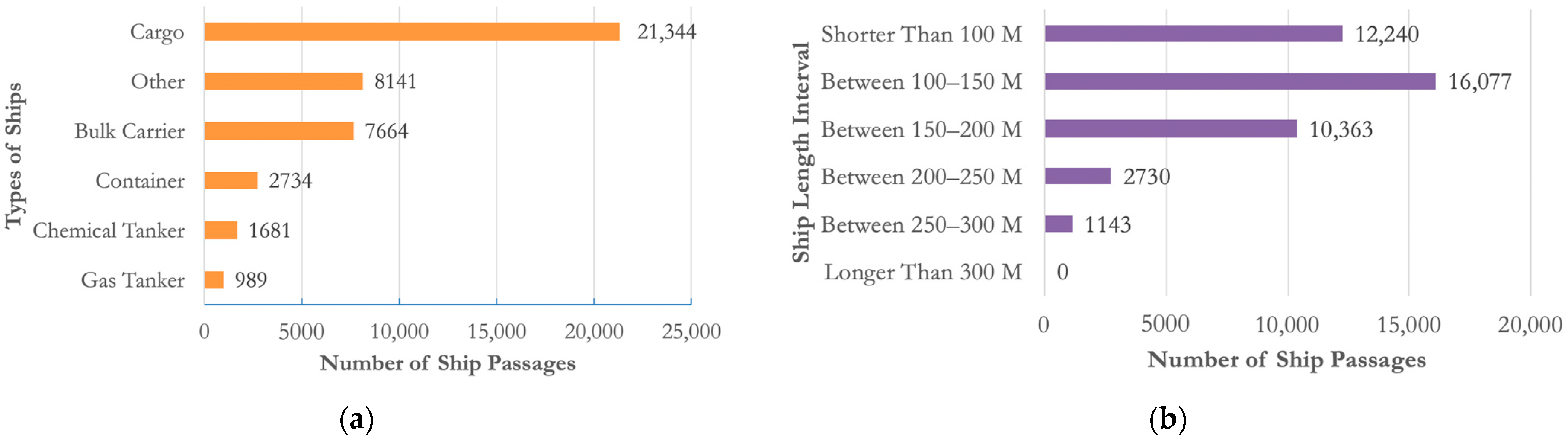
2.2. Application Area

A long-term AIS dataset is utilized in the scope of this study, which is captured from the Strait of Istanbul (SOI). This part presents a general view of the application area and data duration.
The Strait of Istanbul is one of the busiest and most complex waterways around the world. Navigational complexity is driven by the combination of local/transit traffic, continuously varying current regimes, strict maneuvers and narrow sections of the waterway. These are amplified with the crossing scheme, which meets two traffic routes in the busiest section of the straight [40]. With maritime traffic exceeding 300,000 vessels [40], complexity affects ship–ship interactions significantly.
In Figure 1a, yearly descriptive statistics about the types of ships passing through the SOI are presented. In Figure 1b, the distribution of length intervals for ships is presented. The largest percentage of the ships are comprised of cargo ships. When the ship length intervals are examined, the largest number of ships are present at 100–150 m intervals.
To obtain the full picture of the waterway traffic, 1 year of AIS data have been analyzed, covering a time range between September 2014 and August 2015. AIS data messages are stored and managed through Structured Query Language (SQL), with a size of 94 Gigabytes (GB). Detailed information about the data collection, initial management and organization process can be found in Altan and Otay [40].

3. Conceptual Basis

The scalable and interpretable nature of a clustering model with few variables would be a basis to pioneer discussions on observational insights based on clustering outcomes. Since one of the objectives of this study is to identify patterns in risky encounters, showing the relevance of used variables has been a prioritized objective. However, challenges are present for an innovative method’s potential applicability as a software system to maritime navigation systems [41]. On this basis, the clustering model is structured so that it can be tested without needing a complex computational system or runtime and with relatively few features. Considering the studies in the literature, the main risk parameter is taken as the ship domain violation. Own ship’s length and the target ship’s speed are used as the clustering model variables. In this section, the risk parameter and clustering variables are explained as subsections.

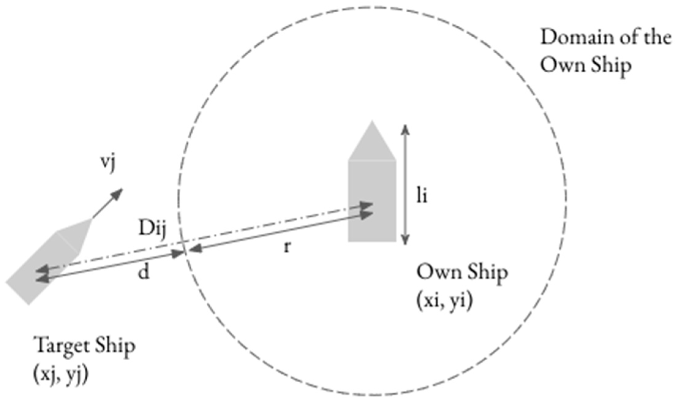
3.1. Ship Domain Violation

Fujii and Tanaka [42] suggested that the ship domain is an area from which target ships must avoid. On the other than, recent studies show that violation of the ship domain may not lead to a risky situation, considering a safe passage at a close distance with complete control [15]. Rawson and Brito [25] demonstrated a critique of ship domain-based assessment and risk and noted potential caveats. While researchers [7,43] showed that narrow waterways have complex conditions resulting in locally designated safe encounter conditions. A potential result is site-specific conditions-based ship domains [44]. Altan and Meijers [45] proposed a ship domain for the SOI in this perspective. The study [45] showed the areas around central ships that surrounding ships tended to avoid in the SOI, and the mentioned ship domain model is used in this research. The applied ship domain for the proposed model resembles the natural conditions. It signifies those ships violating these naturally identified areas are subject to a violation that is not naturally observed in ship–ship interactions of the SOI. These can be interpreted as potential maritime conflicts with respect to site-specific conditions.

3.2. Model Variables

Congested waterways bring both transit and local ships together in close proximity. The most distinctive aspect of these types of marine vessels can be mentioned as their length, considering the large sizes of cargo ships, bulk carriers and tankers. At the same time, local ships have smaller sizes and are mainly used as a means of public transportation. Since transit ships are subject to strict speed limit constraints, local ships’ speeds are found to be more diverse. On these bases, this article aims to highlight how the speed of a target ship is determinative in understanding an encounter’s risk aspect, considering the size of the own ship as a parameter for the target ship’s crew. Consequently, the target ship’s speed and its own ship’s length are determined as model variables.
Degré and Lefévre [46] have been the first to propose the usage of velocity in the maritime field in the context of determining the collision risk. In addition, Lenart [47] also contributed to the integration of velocity to determine collision danger via collision threat parameter area (CTPA), based on the idea that the velocity of the subject ship falls into CTPA. Velocity has been integrated as a basis for linear velocity obstacle (Linear-VO) models to detect if the subject ship’s velocity falls into the dedicated zone of velocity obstacle. This is generated by the model by Chen et al. and Kuwata et al. [13,48], where VO is integrated with COLREGs (Convention of International Regulations for Preventing Collisions at Sea) to develop a motion planning algorithm for unmanned surface vessels (UAV). Chen et al. [13] suggested a time discrete non-linear velocity obstacle (TD-NLVO) method to detect collision candidates. While the velocity obstacle (VO) approach is based on a spatio-temporal relationship among objects, the basis for the proposed model is the utilization of the velocity of the target ship at the closest distance to its own ship. This enables us to validate if speed can be a risky encounter parameter in predicting the potential near-miss situation or not.
Zhang et al. [17] have applied ship length as a decision parameter, both directly and indirectly, via the ship domain approach and reached the outcome that vessel size is a significant indicator for a possible near-miss situation’s detection via classifying ships’ size into three clusters. The local and transit maritime traffic characteristics of narrow waterways are distinct. Moreover, there is a significant difference between local ships’ sizes and transit ships’ sizes [40]. Due to this, it has been relevant to include ship size as a decision factor for other ships in interaction. Furthermore, this study also describes the understanding of the own ship’s length by surrounding vessels. One hypothesis can be outlined as local ships’ captains being “more cautious” in certain conditions where transit ships’ observable characteristics resemble intimidation. This is also outlined via varying ship domains based on speed, length, vessel type, course over ground (COG), and approaching angles [45], including ship length as a feature to contribute to detecting the outcome of this hypothesis as well.

4. Materials and Methods

In this part, the framework of the procedure, encounter model and clustering is summarized. Through the framework, significant steps to develop the course are highlighted. In the encounter model section, the most fundamental stage of development of the computational model to extract intelligence out of the ship–ship interaction situations is discussed. Moreover, the utilized ship domain approach to assessing risky encounter determination is provided. Feature selection and design of risky encounter assessment features are outlined. Furthermore, a sample preprocessed dataset is presented. In the Clustering section, the determination of the appropriate algorithms and practical optimality tests are explained. Additionally, the aspect of three-dimensional interpretation and the conceptual basis is demonstrated on the literature basis.

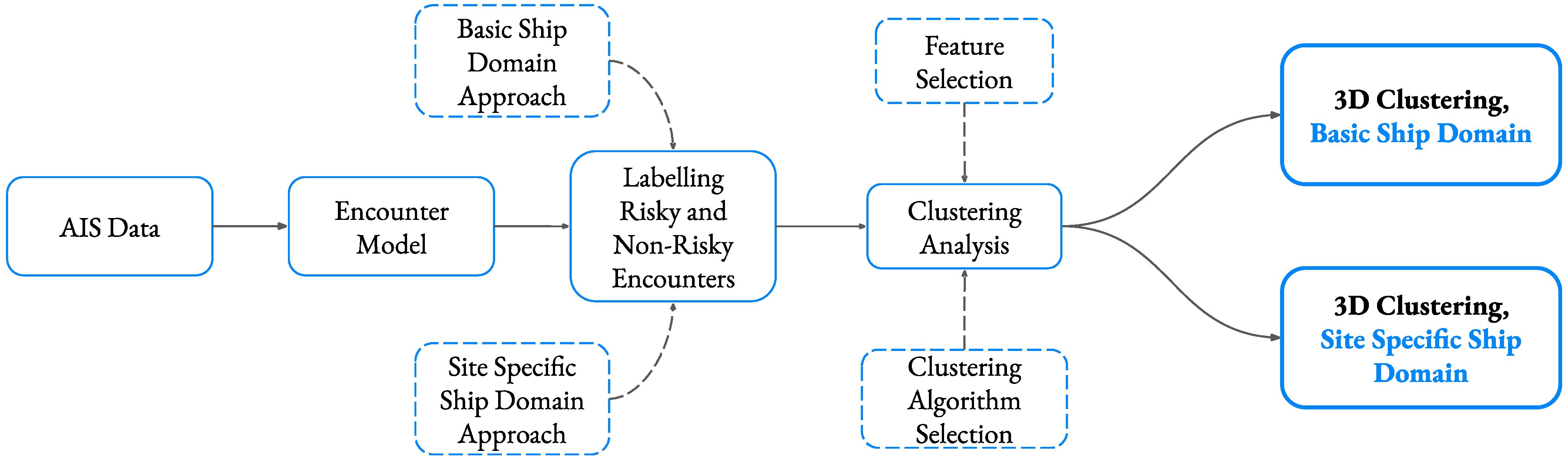
4.1. Framework of the Procedure

Throughout the analysis, different methodologies are combined constructively. In the initial step, an algorithm is developed to transform the raw AIS dataset to an encounter model, where each ship–ship interaction is extracted with respective parameters. Next, based on an extensive literature review and experimental calculations, variables are selected and designed to be introduced to the clustering model. Determination of the used clustering algorithm is also conducted. Based on variables chosen and predetermined algorithms, an optimal number of clusters are calculated via optimality tests, and candidate cluster counts are prepared. In the final step, a three-dimensional clustering application is performed via two distinct ship domain approaches. A high-level diagrammatic representation of the process is provided in Figure 2.

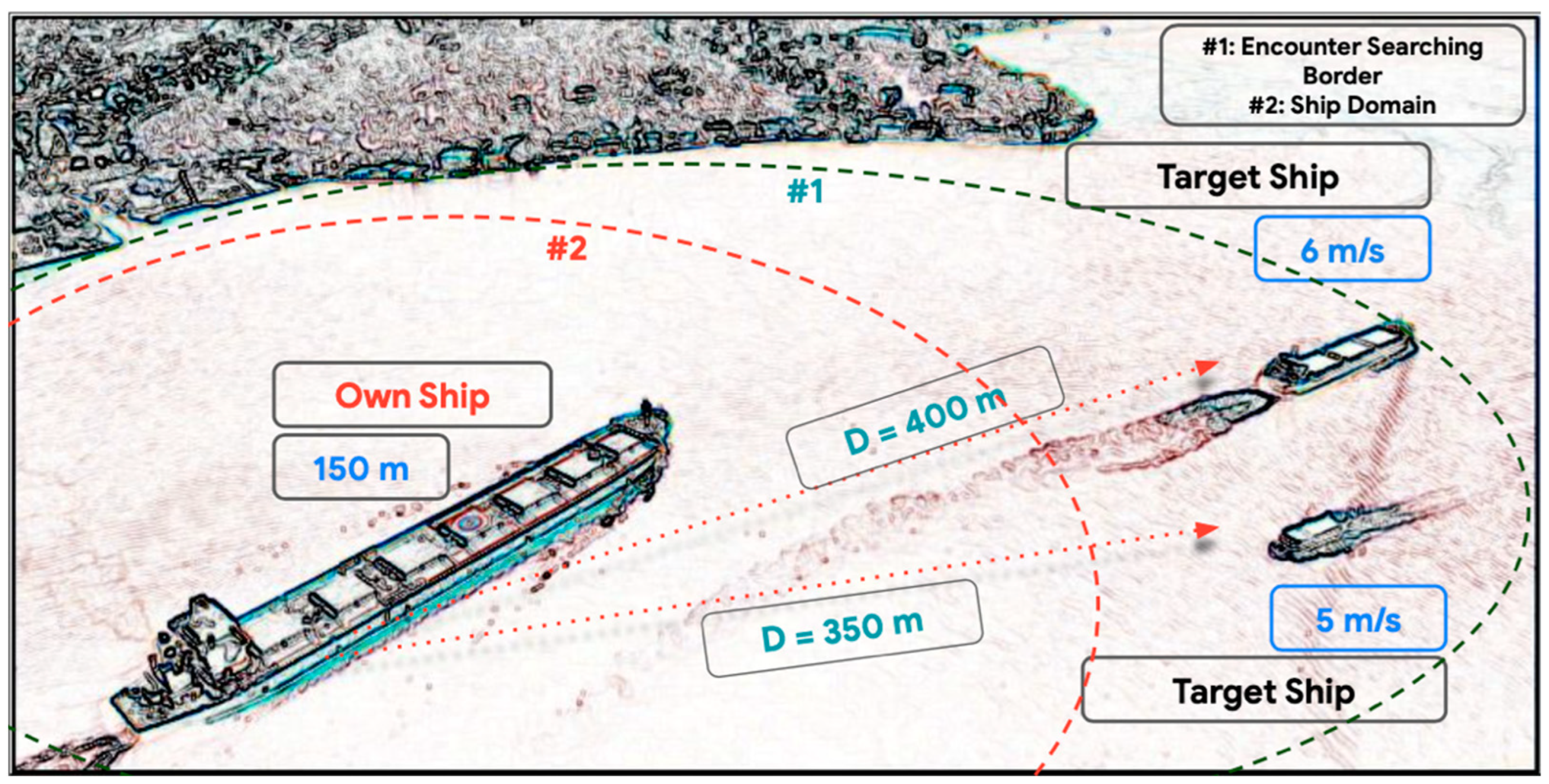
4.2. Encounter Model

A ship–ship encounters database is developed to determine potentially risky encounters. Following an extensive cleaning and preprocessing procedure, algorithms are built and applied to the raw AIS database to create a dataset suitable for the analysis. The resulting dataset has been the basis of clustering applications. Montewka et al.’s [4] circular ship domain, which is also utilized by Weng et al. and Mou et al. [43,49], is adopted. Ship domain violation criteria are used as “Own ship’s domain should not be violated by the entrance of the target ship” [50].
In Figure 3, a representation of the encounter searching algorithm is presented as a sketch in a non-scaled way. A developed algorithm is used to capture the encounter between two ships. Around each own ship, a 1 km meters radius circle is searched. This area is represented with circle #1 in Figure 3. Ships and their distance inside this radius are recorded. Among interactions, the closest interaction between all ships is extracted. Review and elimination of duplicate ship–ship interactions are applied to keep a single interaction between each ship pair. During the application of the algorithm, the non-regular timely submission of data points is overcome via a linear interpolation process. In this way, each interaction situation is analyzed in a synchronized way.
After determining the ship interactions, a smaller circular area is searched around the own vessels. In this step, the radius of the circle is determined through the ship domain of the own ship, and it is demonstrated as circle #2 in Figure 3. For each encounter, the rate of ship domain violation or non-violation is recorded. Through this approach, relevant encounters are recorded, and the dataset is prepared for clustering analysis.
A representation of the ship domain is given in Figure 4. In the Figure, ( x i , y i ) represent own ship’s location, and ( x j , y j ) represent the target ship’s location. l i is the length of the own ship, v j is the velocity of the target ship. Distance between these ships is provided with D i j , where the calculation is given in Equation (1). The radius of the circular ship domain is represented as r , and the distance from the target ship to the domain boundary is shown as d .
D i j =   ( x i x j ) 2 + ( y i y j ) 2  
For the size of the ship domain, Mou et al. [49] state that the majority of circular ship domain radii are around three times the own ship’s length. Based on the unique conditions in the SOI, where narrow passages as low as 700 m are a significant challenge for captains [37], two times the own ship’s length is determined as the basic ship domain approach as given in Equation (2).
r i = 2 × l i
On the other hand, considering the unique conditions of the SOI, a site-specific statistical ship domain approach is used to observe the changes in the results. Therefore, a modified version of the [45] statistical ship domain with two-length groups for the SOI is used. These can be provided as small LOA <= 157 m and large as LOA > 157 m. Smaller ships’ domains were detected to have a lower LOA multiplier for their domain, while larger vessels were observed to have a higher multiplier for their size. To simulate site-specific conditions and represent more accurate ship domain violations, two different ship domain calculations are proposed for respective length groups as given in Equations (3) and (4).
r i = 1.75 × l i   ;   i f   L O A 157   m
r i = 3 × l i   ;   i f   L O A > 157   m
The comparison of the basic ship domain and site-specific ship domain is given in Table 1.
After calculating ship domain distances, the violation of the ship domain for each interaction and violation distances are mapped. Since each interaction’s distance is an essential factor in the violation, a parameter to relate ship–ship distance, violation distance, and own ship’s length is needed. To achieve this, the Violation Distance per Own Ship’s Length (V.D.P.O.S.L.) measure is developed as given in Equation (5):
V . D . P . O . S . L . = l i × r D i j / l i
where l i is the own ship’s length, r is the domain radius for the individual approach, and D i j is the distance between two ships. The V.D.P.O.S.L parameter is critical in the sense that it provides a depth of risk spectrum for model variables. Rather than identifying risky or non-risky situations, the spectrum enables the assessment of risk associated with each encounter smoothly. Moreover, due to the −1 to 1 scale of the variable, encounters that have a value close to 0 are positioned to be neutral, independent of their sign.
V.D.P.O.S.L. parameter also signifies if a ship’s domain is violated or not. Based on similar calculations, this can be represented via a binary relationship as in Equation (6), where x represents own ship’s length:
f x = 0 ,     D i j x × r > 0 1 ,     D i j x × r 0
By using the explained framework, a representation of the prepared dataset used in the clustering analysis is provided in Table 2.

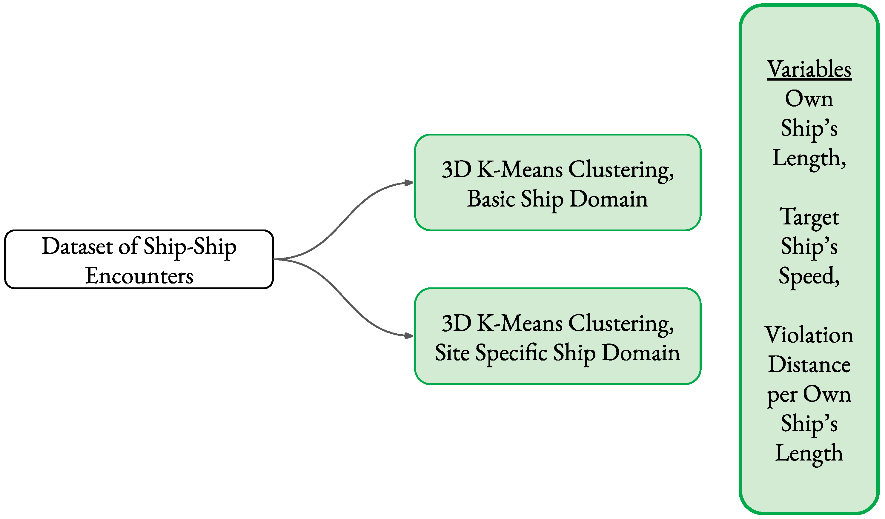
4.3. Clustering Model

Unsupervised learning is generally positioned as the exploratory procedure during an analysis. Moreover, it is identified to be challenging in the sense that assessing the results of an unsupervised learning implementation can be subjective due to the lack of a clear indicator of success [51]. Clustering can be identified as one of the most fundamental unsupervised learning algorithms, convenient where datasets are not naturally labeled and patterns are hidden among the hidden layers. It is also defined as the process of finding out what happens naturally in a given dataset [52]. For the case of vast datasets, if labeling is a challenging process, clustering becomes significantly efficient in discovering insights [53]. Considering the randomness of the encounters, the K-means algorithm is utilized with its computational feasibility, high dimensional convenience and robustness [54].
The k-means algorithm conducts a center-based grouping of provided data points, and each center would represent its group. It is also referred to as “vector quantization,” where the main objective of the algorithm is to apply division to numerous data points for k distinct groups in a way that within-group distances are minimized and distance between members of different groups are maximized [54]. The algorithm works to iterate itself until the centers of the groups would not be subject to further change with each iteration. Additionally, a specific limitation of iterations can be included. Previously, for near-miss modeling, K-means has been used to model spatial images’ clustering to reveal patterns [17]. K-means can be identified as applicable, considering their applicability in visualization and suitability for various shapes to occur due to clustering in the high dimensional space. Since three-dimensional observation is crucial for this research, K-means is suitable to serve.
Since K-means require predetermination of the number of clusters, an initial step for deciding on the optimal number of clusters is needed. Quantitative methodologies to relate the within-cluster sum of distances and the inter-cluster sum of lengths are helpful in conducting judgments. Silhouette Coefficient and Elbow Method are utilized in the scope of this paper. Silhouette can be defined as the measure of within closeness and between apartness of each cluster. This can be expressed as a natural separation assessment for each cluster; in other words, it assesses if the resulting clustering scheme reflects the natural conditions. To calculate Silhouette, the average dissimilarity of a point to its cluster and average dissimilarity to other clusters would be required metrics. It is calculated for each data point, and each score from a dataset can be averaged to assign a Silhouette score for a given dataset in a given number of clusters status. Secondly, elbow methodology measures the sum of squares of each data point to its cluster center [55]. A higher number of clusters may be potentially more explanatory to identifying detailed patterns in a dataset. However, a lower number of clusters could be more insightful and practical for observing distinct separations. Via the elbow method, the optimal point for these two assessments is compared in a two-dimensional plot, and the number of clusters can be decided. While clustering is an analysis that is highly dependent on the approach and can accommodate subjectivity, visual observation is also helpful in assessing optimality in some clusters.
For the cases where quantitative methodologies do not propose an obvious outcome, visual exploration and comparison via domain knowledge are required, as is also applied in this paper [56]. In this perspective, the optimum candidate number of clusters is generated and presented in this study rather than selecting a single number of clusters. This can also be identified as a remark on the subjective nature of clustering analysis, especially in higher dimensions [53]. High dimensional clustering is known for its interpretable challenges and lack of visual observational suitability [57]. The third dimension in clustering helps with an additional observational layer for analysis. At the same time, it does not suffer from a lack of interpretability; instead, it increases the revealing ability of results, so it is advantageous from multiple perspectives.

5. Results and Discussion

The presented approach is applied to a comprehensive AIS dataset collected from the Strait of Istanbul. After the extensive encounter model development process, a clustering dataset has been prepared. Three variables are determined to be input for the clustering model, namely, Own Ship’s Length (0 to 1), Target Ship’s Speed (0 to 1) and Violation Distance per Own Ship’s Length (V.D.P.O.S.L.) (−1 to 1). The −1 to 0 range for V.D.P.O.S.L. should be interpreted as the situation of the ship domain being violated. The 0 to 1 range for the same scale should be interpreted as the ship domain not being violated. Moreover, −1 represents the maximum distance between ships with respect to their own ship’s length, and +1 represents the minimum distance with respect to their own ship’s length. Own Ship’s Length is scaled between 10 m and 300 m. Target Ship’s Speed is scaled between 2 m/s to 15 m/s.
A total of 73,543 interactions are included in the three-dimensional clustering process. Figure 5 represents a general overview of the process.
In the first clustering model, the basic ship domain approach is utilized, as provided in Equation (2). To detect the optimum number of clusters, Silhouette Coefficient and elbow analyses have been conducted. In the Silhouette analysis, 2 clusters obtained the highest score with 0.3651. It was followed by 3 clusters with the second-highest score of 0.3183 and 4 clusters with 0.3143. Moreover, combined with a visual observation for different clusters and the elbow analysis, local optimums in 3, 5 and 9 are selected as candidate numbers of clusters. Silhouette analysis results can be found in Figure 6a. In Figure 6b, the elbow method’s outcome is presented.
In the second clustering model, site-specific ship domain conditions are used as provided in Equations (3) and (4). Silhouette Coefficient resulted in two possible optimum locations, 3 clusters and 5 clusters, with 0.3703 and 0.3027 scores, respectively. Following an elbow analysis and observational judgment, a number of clusters are designated based on these two alternatives, 3 and 5 clusters. Figure 7a,b represent the Silhouette coefficient and elbow model’s graphs for site-specific ship domain conditions, respectively.
Figure 8 and Figure 9 represent three-dimensional clustering visualizations, and in each figure, x, y, z dimensions represent:
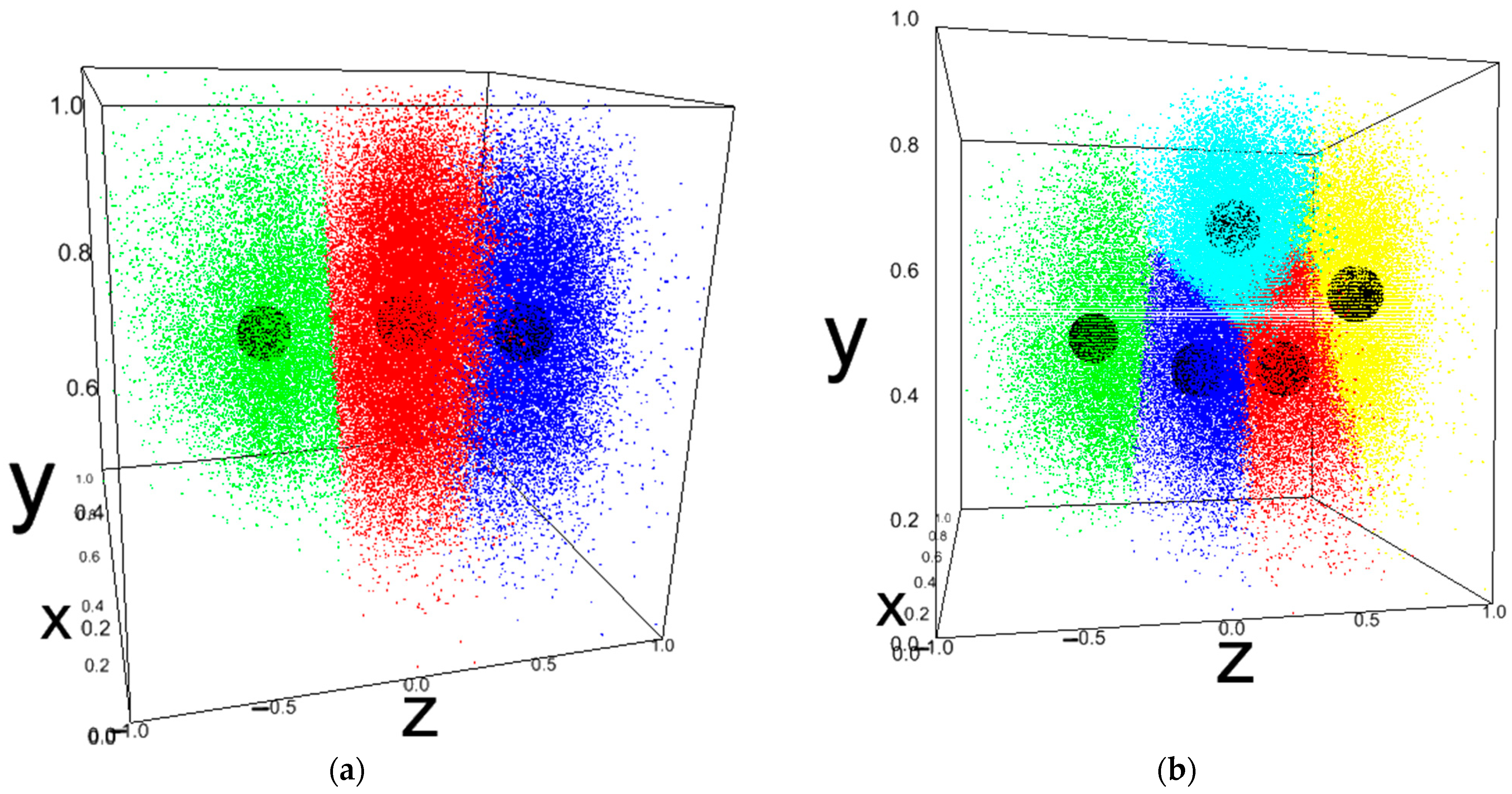
  • x = Own Ship’s Length, Scaled (0 to 1)
  • y = Target Ship’s Speed, Scaled (0 to 1)
  • z = Violation Distance per Own Ship’s Length (V.D.P.O.S.L.), Scaled (−1 to 1)
Figure 8 is the representation of the basic ship domain approach, while Figure 9 is the representation of the site-specific ship domain approach. In Figure 8a and Figure 9a, 3 clusters case is presented for two different ship domain approaches. Figure 8b and Figure 9b represent 5 cluster cases. Finally, 9 cluster cases are presented in Figure 8c. In all visuals, colors are randomly assigned and do not have an underlying implication.
When all clustering outcomes are examined, the mutual pattern can be identified as the mid-cluster, where a smooth trend of switching from non-violation to violation is observed. As the z-axis represents the Violation Distance per Own Ship’s Length parameter, a certain group of interactions that can be defined as almost violations and almost non-violations are observed to be carrying similar properties. So, they form a cluster together. This cumulation around point 0 in the z-axis can be interpreted with the indefinite or ambiguous transition between violation and non-violation situations between ships. In other words, this is the grey zone, which is the end-product of captains’ judgments about the risk. When a ship domain is applied to label these encounters, some of them are labeled as non-risky, although they are very close to risky encounters. As a result, the classification of each ship–ship encounter is binary in terms of risk can be expressed to be challenged with this result.
Edges of clustering results in the z dimension explain how limiting properties are shaped in ship–ship interactions. While there is an unclear separation between violation and non-violation situations in the 0 line, both edges are distinctly clustered together with some data points in the mid-cloud. Considering the three-dimensional plot, the main distinction between interactions is almost always the Violation Distance per Own Ship’s Length, as provided.
In Figure 8, the dispersion of ship–ship encounters in three dimensions is visualized from the own ship’s length perspective. With the increase in the number of clusters for the basic ship domain between Figure 8a,b, the violation indicating cluster gets smaller. The mid-cloud gets divided, and the non-violation cluster gets divided into two parts: one is in the middle of the violation rate while the other is in the far-right edge. The interpretation of this point is how edge points are not being impacted by the change in the number of clusters and how the middle cluster is being further divided. At this point, since the majority of interactions are in the region where violation to non-violation switch occurs, a further separation within this group is being required by maximization of between clusters and minimization of within-cluster principles. At the same time, with 5 clusters, the far-right cluster gets to be divided into the vertical axis (target ship’s speed). This can be explained as the target ship’s speed being a more crucial determinant than the own ship’s length for the case of non-risky interactions. In Figure 8c, nine clusters case is presented. The occurrence of the far left risky clusters is observed. Moreover, in the nine clusters case, only 8 clusters are visible from the x perspective. This indicates how the own ship’s length becomes crucial in the nine clusters case; thus, some of the clusters experience separation in the x perspective.
With the implementation of a site-specific ship domain, more realistic outcomes are attempted, and results are presented in Figure 9a,b. As a result of the implementation, more data points are found out be belonging to the risky encounter class when compared to the basic ship domain. Figure 9a represents the three clusters case, where increased encounters on the negative z-axis are observed. At the same time, based on a general comparison between basic ship domain and site-specific ship domain approaches for five cluster cases, a slight change towards the negative sign in the z-axis is observed in the cluster centers. This can be understood as the impact of site-specific ship domain and the realistic outcome being riskier in the generous sense when a more accurate ship domain approach is implemented.
In addition to the visual representation of the clustering, results are also shown in Table 3 and Table 4 in terms of clusters’ centers for each analysis. Fitted centers are demonstrated to detect risky encounters and corresponding model variable values for their fitted centers. In Table 3, basic ship domain approach, the highest target ship speed is observed in the violation occurring cluster’s center. While the risky encounter cluster is also represented by the lowest own ship’s length value. This indicates that the target ship’s speed and own ship’s length are important determinants of ship domain violation as they represent two edges for both features. In Table 3, five clusters setting, the risky encounter cluster is also observed with the highest target ship speed and lowest own ship’s length. Furthermore, the target ship speed is higher than the three clusters case for this setting. At the same time, in the site-specific ship domain setting, a different pattern is observed. Violation representing cluster is identified by the highest own ship’s length value. This result shows how used decision criteria shapes outcomes, and model variables are representative of risky encounter from different perspectives in varying settings.
Results indicate that the most distinctive axis is the z-axis, which is the defined metric. It would indicate that while length and speed present a diverse distribution, theirs are rather uniform, while V.D.P.O.S.L. metric segments encounter different groups. In other words, the defined metric is a proxy parameter to understand the encounters’ nature about involved risk, and occurring clusters along 0 value indicate encounters should not be solely defined as risky or non-risky; rather, the risk is a continuous measure.
When the overall results of both the B.S.D and S.S.S.D approaches are analyzed, the clustering approach shows the middle clusters, which are at standing close to the ship domain violation, have members both at the violating and non-violating side of the domain boundary. This outcome proves that captains make their judgments according to visual inspection. As a result, ship domain violation is found to be a grey zone rather than a bold line. This outcome can help while making judgments about the risk level of the encounters.

6. Conclusions

In this paper, a novel methodology to explore patterns in ship–ship interactions is presented and applied to the Strait of İstanbul. Three-dimensional clustering analysis is conducted to present patterns among risky encounters. For clustering purposes, the K-means algorithm is used. The number clusters were determined via the elbow and Silhouette method. Visual feature-based mapping for 73,543 encounters is presented, and feature-based separation of risky and non-risky encounters is discussed. The main contribution of this paper is mapping synchronous states of ship speed and ship length in encounter situations together with varying degrees of risk. Ship domain violation per ship’s length is presented as a criterion to assess the severity of the risky encounter and integrated into a three-dimensional clustering analysis.
Results show that both the own ship’s length and the target ship’s speed provide important outcomes in interpreting risky encounters. A cluster of risky encounters forms in each result. For the basic ship domain approach, the lowest own ship’s length and highest target ship speed represent the risky cluster. For the site-specific ship domain approach, the highest own ship’s length represents a risky encounter cluster. The distinction between risky and non-risky encounters is found to obtain a smooth transition. The Violation Distance per Own Ship’s Length (V.D.P.O.S.L.) feature is the most distinctive feature among the presented model features. Basic and site-specific ship domain approaches are used, and both present similar results. The site-specific ship domain highlights risky encounters and produces a greater risky encounter cluster. In all results, the largest cluster occurs in the middle area, where the smallest Violation Distance per Own Ship’s Length values is present. The mid-clusters show that violation is a grey zone rather than a bold line for both basic ship domain and site-specific ship domain applications. Thus, labeling encounters via just ship domain can create over or under-estimation of risky encounters.
A limitation of the study can be described as the lack of individual ship-level information due to the analysis of a large number of encounters. On this basis, the study aims to demonstrate the large-scale occurrence of risky patterns and approach encounters independent of their case-by-case nature.
The study can be improved by including additional model variables and cross-comparison of different variable relationships via clustering. Alternative risky encounter detection frameworks can be applied. The presented model can be applied to different narrow and congested waterways to compare results. Since patterns of risk in terms of model variables are presented, site-specific risk thresholds for model variables can be determined, and these thresholds can be compared between different narrow and congested waterways. In this way, characteristic and quantitative maritime traffic conditions of different sites can be determined. This information can be utilized for maritime traffic regulation through authorities. A ship domain, which has been agreed upon for the given waterway, with all of its irregularities in terms of shape, can be used for further clustering purposes and sensitivity checks of different ship domain sizes can be conducted. Lastly, machine learning-based prediction models can be built to predict risky encounters without including distance by examining ship length and speed as distinctive risk factors. This promising application can help to predict potential risky encounters before vessels enter the waterway.

Author Contributions

Conceptualization, M.F.O. and Y.C.A.; methodology, M.F.O. and Y.C.A.; software, M.F.O.; validation, M.F.O.; formal analysis, M.F.O. and Y.C.A.; investigation, M.F.O. and Y.C.A.; resources, M.F.O. and Y.C.A.; data curation, M.F.O.; writing—original draft preparation, M.F.O. and Y.C.A.; writing—review and editing, M.F.O. and Y.C.A.; visualization, M.F.O.; supervision, Y.C.A.; project administration, Y.C.A. All authors have read and agreed to the published version of the manuscript.

Funding

This research received no external funding.

Data Availability Statement

Readers can access our data by sending an email to the corresponding author.

Conflicts of Interest

The authors declare no conflict of interest.

References

  1. Wan, Z.; Chen, J.; El Makhloufi, A.; Sperling, D.; Chen, Y. Four routes to better maritime governance. Nature 2016, 540, 27–29. [Google Scholar] [CrossRef]
  2. Goerlandt, F.; Goite, H.; Banda, O.A.V.; Höglund, A.; Ahonen-Rainio, P.; Lensu, M. An analysis of wintertime navigational accidents in the Northern Baltic Sea. Saf. Sci. 2017, 92, 66–84. [Google Scholar] [CrossRef]
  3. Qu, X.; Meng, Q.; Suyi, L. Ship collision risk assessment for the Singapore Strait. Accid. Anal. Prev. 2011, 43, 2030–2036. [Google Scholar] [CrossRef]
  4. Montewka, J.; Hinz, T.; Kujala, P.; Matusiak, J. Probability modelling of vessel collisions. Reliab. Eng. Syst. Saf. 2010, 95, 573–589. [Google Scholar] [CrossRef]
  5. Kujala, P.; Hänninen, M.; Arola, T.; Ylitalo, J. Analysis of the marine traffic safety in the Gulf of Finland. Reliab. Eng. Syst. Saf. 2009, 94, 1349–1357. [Google Scholar] [CrossRef]
  6. Mostafa, M.M. Forecasting the Suez Canal traffic: A neural network analysis. Marit. Policy Manag. 2004, 31, 139–156. [Google Scholar] [CrossRef]
  7. Wu, X.; Mehta, A.L.; Zaloom, V.A.; Craig, B.N. Analysis of waterway transportation in Southeast Texas waterway based on AIS data. Ocean Eng. 2016, 121, 196–209. [Google Scholar] [CrossRef]
  8. Mazaheri, A.; Montewka, J.; Kujala, P. Modeling the risk of ship grounding—A literature review from a risk management perspective. WMU J. Marit. Aff. 2013, 13, 269–297. [Google Scholar] [CrossRef]
  9. Kum, S.; Sahin, B. A root cause analysis for Arctic Marine accidents from 1993 to 2011. Saf. Sci. 2015, 74, 206–220. [Google Scholar] [CrossRef]
  10. Pallotta, G.; Vespe, M.; Bryan, K. Vessel Pattern Knowledge Discovery from AIS Data: A Framework for Anomaly Detection and Route Prediction. Entropy 2013, 15, 2218–2245. [Google Scholar] [CrossRef]
  11. Otay, E.N.; Özkan, Ş. Stochastic Prediction of Maritime Accidents in the strait of Istanbul. In Proceedings of the 3rd International Conference on Oil Spills in the Mediterranean and Black SEA Regions, Istanbul, Turkey, 31 October–3 November 2003; pp. 92–104. [Google Scholar]
  12. Merrick, J.R.W.; van Dorp, J.R.; Mazzuchi, T.; Harrald, J.R.; Spahn, J.E.; Grabowski, M. The Prince William Sound Risk Assessment. INFORMS J. Appl. Anal. 2002, 32, 25–40. [Google Scholar] [CrossRef]
  13. Chen, P.; Huang, Y.; Mou, J.; van Gelder, P. Ship collision candidate detection method: A velocity obstacle approach. Ocean Eng. 2018, 170, 186–198. [Google Scholar] [CrossRef]
  14. Tu, E.; Zhang, G.; Rachmawati, L.; Rajabally, E.; Huang, G.-B. Exploiting AIS Data for Intelligent Maritime Navigation: A Comprehensive Survey From Data to Methodology. IEEE Trans. Intell. Transp. Syst. 2017, 19, 1559–1582. [Google Scholar] [CrossRef]
  15. Du, L.; Goerlandt, F.; Kujala, P. Review and analysis of methods for assessing maritime waterway risk based on non-accident critical events detected from AIS data. Reliab. Eng. Syst. Saf. 2020, 200, 106933. [Google Scholar] [CrossRef]
  16. Debnath, A.K.; Chin, H.C. Navigational Traffic Conflict Technique: A Proactive Approach to Quantitative Measurement of Collision Risks in Port Waters. J. Navig. 2009, 63, 137–152. [Google Scholar] [CrossRef]
  17. Zhang, W.; Goerlandt, F.; Kujala, P.; Wang, Y. An advanced method for detecting possible near miss ship collisions from AIS data. Ocean Eng. 2016, 124, 141–156. [Google Scholar] [CrossRef]
  18. Debnath, A.; Chin, H.C. Analysis of marine conflicts. In Proceedings of the 19th KKCNN Symposium on Civil Engineering, Kyoto, Japan, 10–12 December 2006. [Google Scholar]
  19. Zhang, W.; Goerlandt, F.; Montewka, J.; Kujala, P. A method for detecting possible near miss ship collisions from AIS data. Ocean Eng. 2015, 107, 60–69. [Google Scholar] [CrossRef]
  20. Zhang, W.; Feng, X.; Goerlandt, F.; Liu, Q. Towards a Convolutional Neural Network model for classifying regional ship collision risk levels for waterway risk analysis. Reliab. Eng. Syst. Saf. 2020, 204, 107127. [Google Scholar] [CrossRef]
  21. Rong, H.; Teixeira, A.; Soares, C.G. Spatial correlation analysis of near ship collision hotspots with local maritime traffic characteristics. Reliab. Eng. Syst. Saf. 2021, 209, 107463. [Google Scholar] [CrossRef]
  22. Watawana, T.; Caldera, A. Analyse Near Collision Situations of Ships Using Automatic Identification System Dataset. In Proceedings of the 2018 5th International Conference on Soft Computing & Machine Intelligence (ISCMI), Nairobi, Kenya, 21–22 November 2018; pp. 155–162. [Google Scholar] [CrossRef]
  23. Li, Y.-P.; Liu, Z.-J.; Kai, J.S. Study on complexity model and clustering method of ship to ship encoun-tering risk. J. Mar. Sci. Technol. 2019, 27, 153–160. [Google Scholar] [CrossRef]
  24. Szlapczynski, R.; Szlapczynska, J. A ship domain-based model of collision risk for near-miss detection and Collision Alert Systems. Reliab. Eng. Syst. Saf. 2021, 214, 107766. [Google Scholar] [CrossRef]
  25. Rawson, A.; Brito, M. A critique of the use of domain analysis for spatial collision risk assessment. Ocean Eng. 2020, 219, 108259. [Google Scholar] [CrossRef]
  26. Öztürk, Ü.; Boz, H.A.; Balcisoy, S. Visual analytic based ship collision probability modeling for ship navigation safety. Expert Syst. Appl. 2021, 175, 114755. [CrossRef]
  27. Du, L.; Banda, O.A.V.; Goerlandt, F.; Huang, Y.; Kujala, P. A COLREG-compliant ship collision alert system for stand-on vessels. Ocean Eng. 2020, 218, 107866. [Google Scholar] [CrossRef]
  28. Goerlandt, F.; Kujala, P. On the reliability and validity of ship–ship collision risk analysis in light of different perspectives on risk. Saf. Sci. 2014, 62, 348–365. [Google Scholar] [CrossRef]
  29. Weng, J.; Liao, S.; Wu, B.; Yang, D. Exploring effects of ship traffic characteristics and environmental conditions on ship collision frequency. Marit. Policy Manag. 2020, 47, 523–543. [Google Scholar] [CrossRef]
  30. Fang, Z.; Yu, H.; Ke, R.; Shaw, S.-L.; Peng, G. Automatic Identification System-Based Approach for Assessing the Near-Miss Collision Risk Dynamics of Ships in Ports. IEEE Trans. Intell. Transp. Syst. 2019, 20, 534–543. [Google Scholar] [CrossRef]
  31. Debnath, A.K.; Chin, H.C. Modelling Collision Potentials in Port Anchorages: Application of the Navigational Traffic Conflict Technique (NTCT). J. Navig. 2015, 69, 183–196. [Google Scholar] [CrossRef]
  32. Liu, K.; Yuan, Z.; Xin, X.; Zhang, J.; Wang, W. Conflict detection method based on dynamic ship domain model for visualization of collision risk Hot-Spots. Ocean Eng. 2021, 242, 110143. [Google Scholar] [CrossRef]
  33. Feng, H.; Grifoll, M.; Yang, Z.; Zheng, P. Collision risk assessment for ships’ routeing waters: An information entropy approach with Automatic Identification System (AIS) data. Ocean Coast. Manag. 2022, 224, 106184. [Google Scholar] [CrossRef]
  34. Zhou, Y.; Daamen, W.; Vellinga, T.; Hoogendoorn, S.P. Ship classification based on ship behavior clustering from AIS data. Ocean Eng. 2019, 175, 176–187. [Google Scholar] [CrossRef]
  35. Wang, J.; Zhu, C.; Zhou, Y.; Zhang, W. Vessel Spatio-temporal Knowledge Discovery with AIS Trajectories Using Co-clustering. J. Navig. 2017, 70, 1383–1400. [Google Scholar] [CrossRef]
  36. Zhang, D.; Zhang, Y.; Zhang, C. Data mining approach for automatic ship-route design for coastal seas using AIS trajectory clustering analysis. Ocean Eng. 2021, 236, 109535. [Google Scholar] [CrossRef]
  37. Mieczyńska, M.; Czarnowski, I. K-means clustering for SAT-AIS data analysis. WMU J. Marit. Aff. 2021, 20, 377–400. [Google Scholar] [CrossRef]
  38. Park, J.; Jeong, J.-S. An Estimation of Ship Collision Risk Based on Relevance Vector Machine. J. Mar. Sci. Eng. 2021, 9, 538. [Google Scholar] [CrossRef]
  39. Rawson, A.; Brito, M. A survey of the opportunities and challenges of supervised machine learning in maritime risk analysis. Transp. Rev. 2022, 43, 108–130. [Google Scholar] [CrossRef]
  40. Altan, Y.C.; Otay, E.N. Maritime Traffic Analysis of the Strait of Istanbul based on AIS data. J. Navig. 2017, 70, 1367–1382. [Google Scholar] [CrossRef]
  41. Ożoga, B.; Montewka, J. Towards a decision support system for maritime navigation on heavily trafficked basins. Ocean Eng. 2018, 159, 88–97. [Google Scholar] [CrossRef]
  42. Fujii, Y.; Tanaka, K. Traffic Capacity. J. Navig. 1971, 24, 543–552. [Google Scholar] [CrossRef]
  43. Weng, J.; Meng, Q.; Qu, X. Vessel Collision Frequency Estimation in the Singapore Strait. J. Navig. 2012, 65, 207–221. [Google Scholar] [CrossRef]
  44. Hansen, M.G.; Jensen, T.K.; Lehn-Schiøler, T.; Melchild, K.; Rasmussen, F.M.; Ennemark, F. Empirical Ship Domain based on AIS Data. J. Navig. 2013, 66, 931–940. [Google Scholar] [CrossRef]
  45. Altan, Y.C.; Meijers, B.M. Ship Domain Variations in the Strait of Istanbul. In Proceedings of the WCTRS SIGA2 2021 Conference, Antwerp, Belgium, 5–7 May 2021. [Google Scholar]
  46. Degré, T.; Lefèvre, X. A Collision Avoidance System. J. Navig. 1981, 34, 294–302. [Google Scholar] [CrossRef]
  47. Lenart, A.S. Collision Threat Parameters for a new Radar Display and Plot Technique. J. Navig. 1983, 36, 404–410. [Google Scholar] [CrossRef]
  48. Kuwata, Y.; Wolf, M.T.; Zarzhitsky, D.; Huntsberger, T.L. Safe Maritime Navigation with COLREGS Using Velocity Obstacles; Institute of Electrical and Electronics Engineers (IEEE): Piscataway, NJ, USA, 2011; pp. 4728–4734. [Google Scholar] [CrossRef]
  49. Mou, J.M.; van der Tak, C.; Ligteringen, H. Study on collision avoidance in busy waterways by using AIS data. Ocean Eng. 2010, 37, 483–490. [Google Scholar] [CrossRef]
  50. Szlapczynski, R.; Szlapczynska, J. Review of ship safety domains: Models and applications. Ocean Eng. 2017, 145, 277–289. [Google Scholar] [CrossRef]
  51. James, G.; Witten, D.; Hastie, T.; Tibshirani, R. An Introduction to Statistical Learning: With Applications in R.; Springer: New York, NY, USA, 2013; p. 426. ISBN 978-1-4614-7137-0. [Google Scholar] [CrossRef]
  52. Barlow, H.; Laboratory, P.L.H.B.C.; Xiong, H.; Rodríguez-Sánchez, A.J.; Szedmak, S.; Piater, J.; Lagorce, X.; Ieng, S.-H.; Clady, X.; Pfeiffer, M.; et al. Unsupervised Learning. Neural Comput. 1989, 1, 295–311. [Google Scholar] [CrossRef]
  53. Alpaydin, E. Introduction to Machine Learning; The MIT Press: Cambridge, MA, USA, 2004. [Google Scholar]
  54. Hartigan, J.A.; Wong, M.A. Algorithm AS 136: A K-Means Clustering Algorithm. J. R. Stat. Soc. Ser. Appl. Stat. 1979, 28, 100–108. [Google Scholar] [CrossRef]
  55. Thorndike, R.L. Who belongs in the family? Psychometrika 1953, 18, 267–276. [Google Scholar] [CrossRef]
  56. Bittmann, R.M.; Gelbard, R.M. Decision-making method using a visual approach for cluster analysis problems; indicative classification algorithms and grouping scope. Expert Syst. 2007, 24, 171–187. [Google Scholar] [CrossRef]
  57. Hastie, T.; Tibshirani, R.; Friedman, J. The Elements of Statistical Learning: Data Mining, Inference, and Prediction; Springer Science & Business Media: New York, NY, USA, 2009. [Google Scholar]
Figure 1. (a) Yearly Ship Type Distribution; (b) Yearly Ship Length Distribution.
Jmse 11 00950 g001
Figure 2. Methodological framework.
Jmse 11 00950 g002
Figure 3. Encounter searching algorithm representation.
Jmse 11 00950 g003
Figure 4. Encounter situation and ship domain as the safety criteria.
Jmse 11 00950 g004
Figure 5. General overview of the clustering process.
Jmse 11 00950 g005
Figure 6. (a) Silhouette Score graph for basic ship domain model; (b) Elbow Method graph for basic ship domain model.
Jmse 11 00950 g006
Figure 7. (a) Silhouette Score graph for site-specific ship domain model; (b) Elbow Method graph for site-specific ship domain model.
Jmse 11 00950 g007
Figure 8. Three-dimensional Clustering with Basic Ship Domain, X perspective (a) 3 clusters case, (b) 5 clusters case, (c) 9 clusters case.
Jmse 11 00950 g008
Figure 9. Three-dimensional Clustering with Site Specific Ship Domain, X perspective (a) 3 clusters case, (b) 5 clusters case.
Jmse 11 00950 g009
Table 1. Respective ship domain radii for two approaches.
Ship Length (m)Basic Ship Domain (m)Site Specific Ship Domain (m)
Length (li) ≤ 157 m2 × li1.75 × li
Length (li) > 157 m2 × li3 × li
Table 2. Dataset used in the clustering process.
VariableValue
Own Ship’s Length (m)157
Target Ship’s Speed (m/s)4.5
Basic Ship Domain (m)157 × 2
Site-specific Ship Domain (m)157 × 1.75
Distance (m)350
Violation Distance per Own Ship’s Length (B.S.D.)((157 × 2) − 350)/157
Violation Distance per Own Ship’s Length (S.S.S.D.)((157 × 1.75) − 350)/157
Violation Indicator (0 or 1) (Basic Ship Domain)0
Violation Indicator (0 or 1) (Site-specific Ship Domain)1
Table 3. Basic Ship Domain Clustering Results: Fitted Centers.
Non-Scaled, Basic Ship Domain
3 Clusters Fitted Centers
Cluster No.Own Ship’s Length (m)Target Ship’s Speed (m/s)V.D.P.O.S.L.
196.8724.821−0.203
2266.9123.7220.573
3139.9283.5620.161
5 Clusters Fitted Centers
Cluster No.Own Ship’s Length (m)Target Ship’s Speed (m/s)V.D.P.O.S.L.
1229.165.4210.278
2109.3523.5020.055
397.8085.275−0.278
4186.7283.2620.348
5284.3843.4890.655
9 Clusters Fitted Centers
Cluster No.Own Ship’s Length (m)Target Ship’s Speed (m/s)V.D.P.O.S.L.
1129.0085.035−0.054
2298.4243.2620.724
376.5923.4420.08
4236.0243.2890.511
591.2565.654−0.39
6117.1523.2490.115
7285.9445.1810.493
8173.6243.2820.302
9205.1365.3150.208
Table 4. Site-Specific Ship Domain Clustering Results: Fitted Centers.
Non-Scaled, Site-Specific Ship Domain
3 Clusters Fitted Centers
Cluster No.Own Ship’s Length (m)Target Ship’s Speed (m/s)V.D.P.O.S.L.
1124.645.0550.15
2207.0084.435−0.312
3109.3524.9210.604
5 Clusters Fitted Centers
Cluster No.Own Ship’s Length (m)Target Ship’s Speed (m/s)V.D.P.O.S.L.
1120.5844.1350.384
2116.2166.1010.163
3105.6085.1810.677
4145.2324.0820.052
5210.444.515−0.359
Disclaimer/Publisher’s Note: The statements, opinions and data contained in all publications are solely those of the individual author(s) and contributor(s) and not of MDPI and/or the editor(s). MDPI and/or the editor(s) disclaim responsibility for any injury to people or property resulting from any ideas, methods, instructions or products referred to in the content.

