Analysis and Compensation of Installation Perpendicularity Error in Unmanned Surface Vehicle Electro-Optical Devices by Using Sea–Sky Line Images

Abstract

As an important sensor of an unmanned surface vehicle (USV), an electro-optical device is usually used to detect ships and obstacles in USV autonomous navigation and collision avoidance. However, the installation perpendicularity error of the electro-optical device greatly impacts the line-of-sight (LOS) stability control. This error is difficult to eliminate through mechanical calibration because the platform inertial navigation axis cannot be led out. This study aims to establish the model for the perpendicularity error of electro-optical devices during circumferential scanning and analyze its impact on the stability of LOS. In addition, we present a measurement technique for perpendicularity errors utilizing sea–sky line images. Through this method, we find an error function of LOS elevation angle, which is a convex function that can quickly search out high-precision perpendicularity errors step by step. Finally, we measured and compensated the perpendicularity error according to experimental data collected by the electro-optical device. The findings of this research demonstrate that the suggested approach can efficiently mitigate low-frequency disruptions and minor amplitude high-frequency vibrations of LOS in the elevation direction. As a result, it considerably enhances the precision of stability and image observation effect of electro-optical devices.

1. Introduction

In recent years, with the rapid developments of unmanned technology, artificial intelligence, and internet technology, unmanned intelligent autonomous systems have been widely used in military and civilian fields. An unmanned surface vehicle [1], as a highly autonomous sea mobile platform, can be employed for large-scale, long-term, low-cost engineering tasks and marine scientific research tasks in the ocean. It can even replace manned platforms to conduct operations in dangerous sea areas or sea conditions [2,3,4]. Hence, unmanned surface vehicles (USVs) have emerged as a crucial research subject in achieving ship intelligence and automation. In non-military applications, USVs primarily serve the purpose of marine environmental monitoring, maritime surveillance and patrol, evidence collection and investigation, search and rescue operations, and elimination of floating debris from the ocean’s surface [5,6,7]. USVs are usually equipped with advanced sensing systems [8], control systems, communication systems, and navigation systems that can accomplish various tasks such as intelligent environmental perception, autonomous planning and decision-making, navigation collision avoidance [4,9,10], and target detection and recognition [11,12,13]. USV sensing systems are mainly composed of electro-optical, radar, sonar, and other devices [14,15]. The electro-optical device can detect and recognize ships and obstacles in the sea and is thus an important means for USVs to achieve navigation collision avoidance, intelligent target awareness, and auxiliary decision-making [16,17,18].

USVs roll and pitch under the influence of surface waves when sailing on the sea. To ensure that the line-of-sight (LOS) of the electro-optical device is not affected by the sway of the hull, the electro-optical device is usually designed with a two-axis stabilization function for the LOS [19]. The hull attitude information provided by the USV inertial navigation equipment is acquired, then used to adjust the rotation of the electro-optical sensor assembly in the azimuth and elevation directions in real time, to reversely compensate for the hull swing to isolate hull disturbance and stabilize the LOS. In principle, the device’s coordinate system of electro-optical equipment should be parallel to the platform’s inertial navigation coordinate system, utilizing the platform’s inertial navigation attitude data. Therefore, during the installation of the equipment on the ship’s deck, the electro-optical device must be leveled and calibrated to ensure consistency between the two coordinate systems. However, in practical terms, extracting and measuring the three axes of the inertial navigation coordinate system is challenging, leading to a deviation between the base plane of the electro-optical device and the horizontal plane of the inertial navigation. Consequently, the azimuth rotation axis of the electro-optical device is not perpendicular to the horizontal plane of the inertial navigation. The perpendicularity error causes an angular deviation between the electro-optical stabilization and the required pointing [20]. For example, when the electro-optical device performs a circumferential scanning at the zero-degree angle of the elevation, the LOS should move along the sea–sky line; however, the actual LOS moves upward and downward around the sea–sky line and vibrates in small amplitude and high frequency. When observing distant scenes in a small viewing field, an image of the sky or the sea may also be included. In view of this phenomenon, we study the influence of LOS stability control in the circumferential scanning process caused by the installation perpendicularity error between the base of the electro-optical device and the platform of USV, and propose an error measurement and compensation method based on sea–sky line images. The simulation and experimental results reveal that the proposed correction method could effectively reduce low-frequency disturbances and small high-frequency vibrations of the LOS and improve the system’s stabilization accuracy.

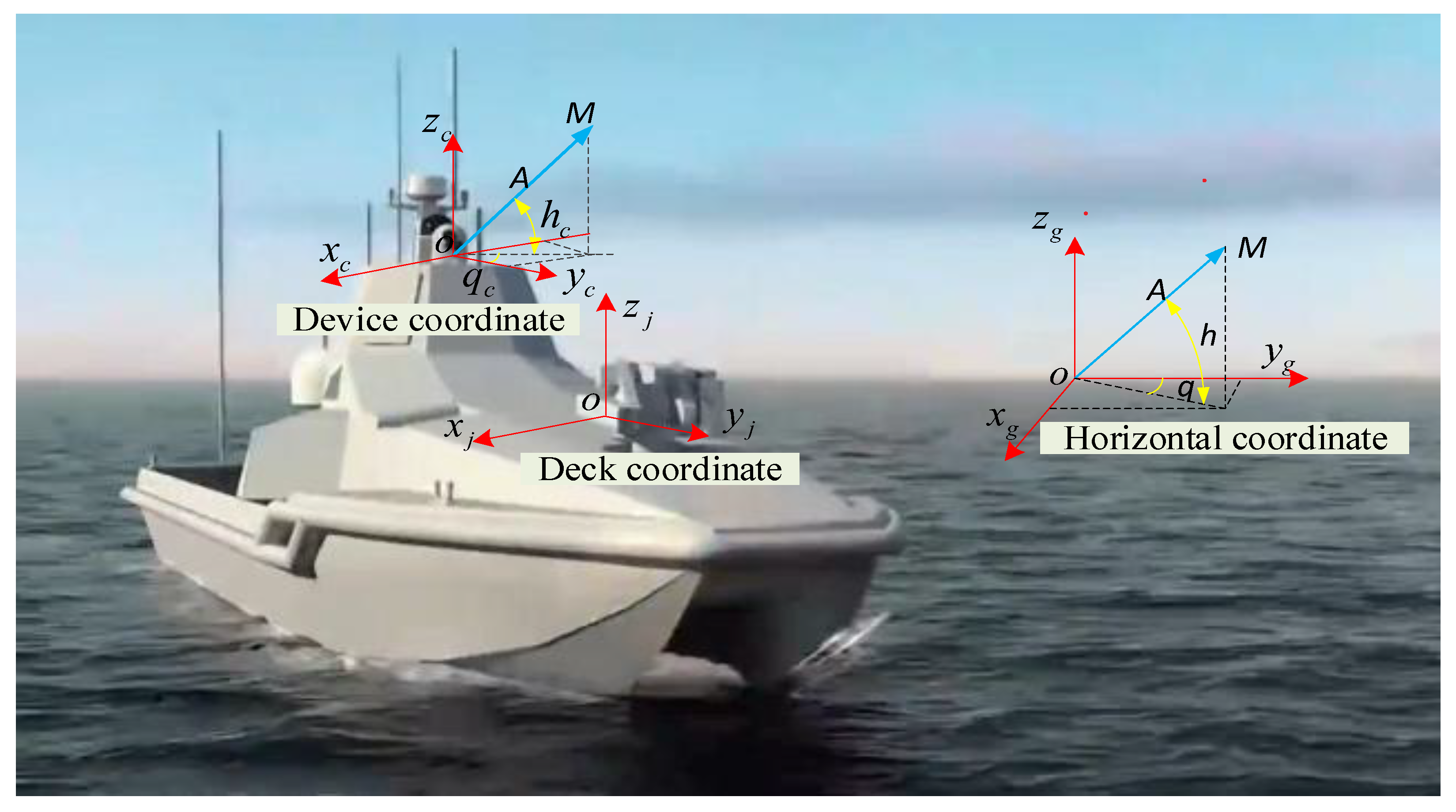
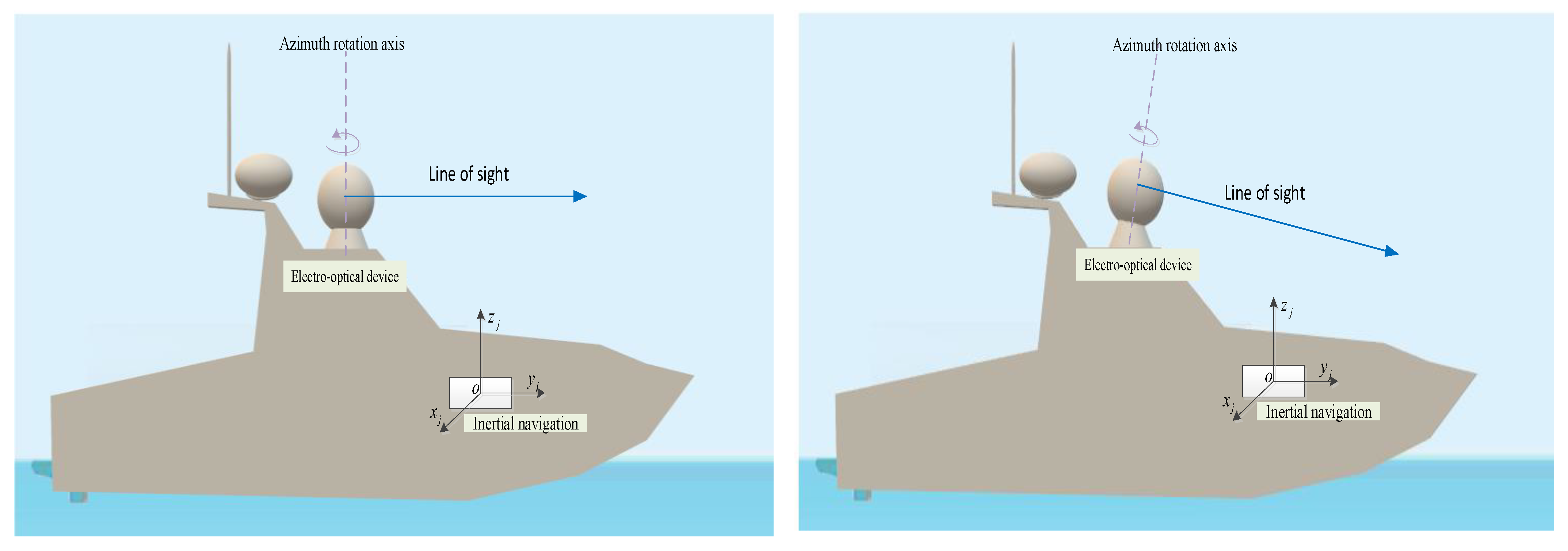
2. LOS Stabilization Representation

As shown in Figure 1, the coordinate system of the electro-optical device installed on the USV and connected with the carrier is $o{x}_c{y}_c{z}_c$. The coordinate system of the deck where the USV inertial navigation base is installed is $o{x}_j{y}_j{z}_j$, where $o{y}_j$, $o{x}_j$, $o{z}_j$ point ship heading, starboard, and upwards, respectively [21]. The horizontal coordinate system is $o{x}_g{y}_g{z}_g$, with $o{y}_g$ pointing due north, $o{x}_g$ pointing due east, $o{z}_g$ facing up, and the $x_{g}o{y}_g$ plane parallel to the earth. The $o{x}_g{y}_g{z}_g$ is the reference coordinate system, and $o{x}_c{y}_c{z}_c$, $o{x}_j{y}_j{z}_j$ are the axis coordinate system of the electro-optical device and inertial navigation device, respectively. These coordinate systems conform to the right-hand rule [22]. When there is no installation perpendicularity error or azimuth initialization error, the $o{x}_c{y}_c{z}_c$ can coincide with $o{x}_j{y}_j{z}_j$ by coordinate system translation.

The matrix expression of the pointing vector $A$ of the LOS M of the electro-optical device in the horizontal coordinate system is as follows:

$$A={(\cos h\sin q,\cos h\cos q,\sin h)}^T$$

(1)

where q and h are the azimuth and elevation angles of the LOS M in the horizontal coordinate system, respectively.

When the hull rotates around the $o{x}_j$ axis by a pitch angle P, the transformation matrix of point M from the horizontal coordinate system to the deck coordinate system can be expressed as follows:

$$S_p=\left[\begin{array}{ccc}1& 0& 0\\ 0& \cos P& \sin P\\ 0& -\sin P& \cos P\end{array}\right]$$

(2)

When the hull rotates around the $o{y}_c$ axis by a roll angle R, the transformation matrix of point M from the horizontal coordinate system to the deck coordinate system can be written as follows:

$$S_R=\left[\begin{array}{ccc}\cos R& 0& -\sin R\\ 0& 1& 0\\ \sin R& 0& \cos R\end{array}\right]$$

(3)

Accordingly, the matrix expression of vector $A$ in the deck coordinate system is as follows:

$$A_j=S_R{S}_{P}A$$

(4)

Furthermore, the azimuth angle $q_j$ and pitch angle $h_j$ of the LOS M in the deck coordinate system after rotation can be, respectively, expressed as follows:

$$q_j={\tan }^{-1}(A_j(1)/A_j(2))$$

(5)

$$h_j={\sin }^{-1}(A_j(3))$$

(6)

Because the device coordinate system $o{x}_c{y}_c{z}_c$ is consistent with the deck coordinate system $o{x}_j{y}_j{z}_j$, the azimuth angle $q_c$ and elevation angle $h_c$ of the LOS M in the device coordinate system are $q_c=q_j \mathrm{and} h_c=h_j$, respectively.

To ensure that the LOS is pointing to $M$ on the sea–sky line, the electro-optical device must be rotated in the azimuth and elevation directions relative to the device coordinate system by angles $\mathsf{\Delta }q=q_c \mathrm{and} \mathsf{\Delta }h=h_c$, respectively. Thus, the shaking of the captured images caused by the swaying of the carrier can be eliminated to realize the LOS stabilization function in the horizontal coordinate system. When the elevation angle $h$ is zero, the center of the images captured by the electro-optical device is always stable on the sea–sky line.

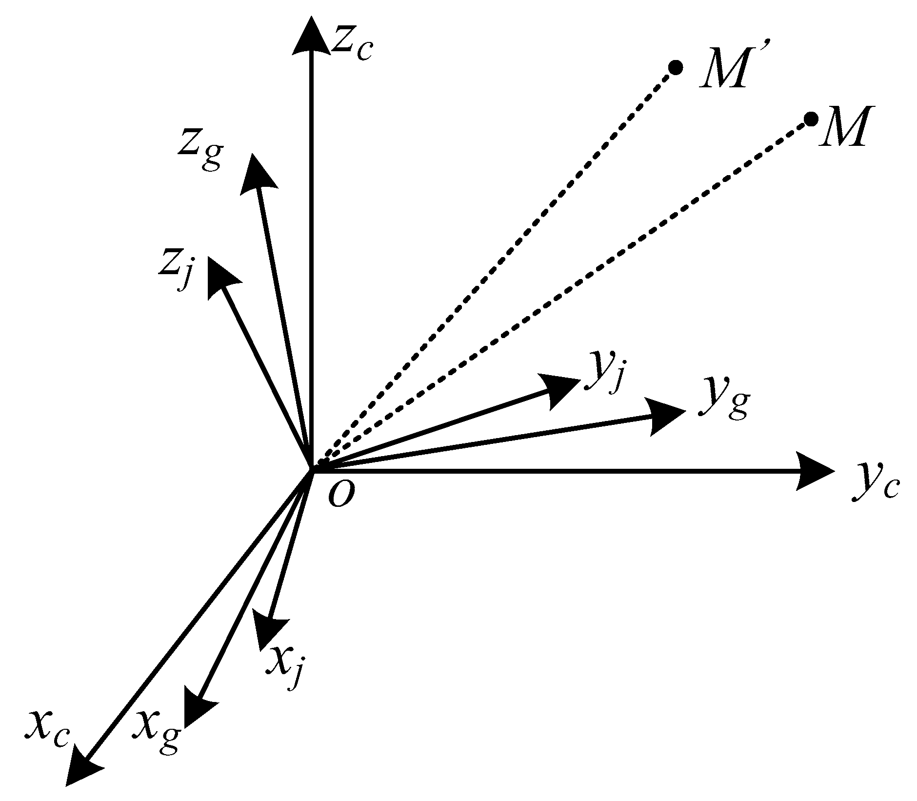
3. Influence of the Perpendicularity Error on Stability

When the electro-optical device is installed on the USV, the base plane of the equipment must be level with the horizontal plane of the platform inertial navigation and aligned with the inertial navigation azimuth so that the coordinate system $o{x}_c{y}_c{z}_c$ of the electro-optical device is parallel to the coordinate system $o{x}_j{y}_j{z}_j$ of the deck [23]. The attitude angle of the hull sensitive to inertial navigation is consistent with the swing angle of the electro-optical device (i.e., the rotation angles of $o{x}_c{y}_c{z}_c$ and $o{x}_j{y}_j{z}_j$ are the same) only when the aforementioned condition is satisfied. The electro-optical equipment compensates for carrier swing by utilizing real-time calculations of the inertial navigation’s attitude data [24,25]. Achieving image stabilization necessitates maintaining consistency between the attitude angle obtained through the boat’s inertial navigation and that of the electro-optical equipment. Where there is an installation perpendicularity error, as shown in Figure 2, the above precondition is violated, and there is a deviation between the attitude angle of the electro-optical device and the inertial navigation sensitive attitude angle. This causes a deviation in the pointing of the LOS in the horizontal coordinate system after compensation.

In the case of a perpendicularity error in the installation of the electro-optical device, the electro-optical azimuth rotation axis $o{z}_c$ is inclined at a certain angle, and a certain space angle exists between the $x_{c}o{y}_c$ and $x_j{o}_{}{y}_j$ planes [26]. Assume that the error angle component relative to the $x_j$ and $y_j$ axes are $\alpha$ and $\beta$, respectively, and the azimuth angle $q_c$ and elevation angle $h_c$ of $M^{\prime }$ in the device coordinate system $o{x}_c{y}_c{z}_c$ are known.

According to Euler’s law of rotation, the real pointing coordinates of the LOS $M^{\prime }$ in this state can be calculated by rotating the vector $M^{\prime }$ by perpendicularity error angles $\alpha$ and $\beta$ from the $o{x}_c{y}_c{z}_c$ coordinate system to the $o{x}_j{y}_j{z}_j$ coordinate system, as shown in Figure 3, and then its coordinate matrix in the horizontal coordinate system can be calculated according to the attitude angle.

(1)

Transformation from the device coordinate system to the deck coordinate system

According to Equations (5) and (6), the coordinate matrix $A_c^{\prime }$ of $M^{\prime }$ in the device coordinate system can be expressed as follows:

$$A_i^{\prime }={(\cos h_c\sin q_c,\cos h_c\cos q_c,\sin h_c)}^T$$

(7)

Then, its coordinate matrix $A_j$ in the deck coordinate system can be obtained through the following transformation:

$$A_j^{\prime }=S_{\alpha }{S}_{\beta }{A}_c^{\prime }$$

(8)

where $S_{\alpha }$ and $S_{\beta }$ are rotation matrices and can be expressed as follows:

$$S_{\alpha }=\left[\begin{array}{ccc}1& 0& 0\\ 0& \cos \alpha & -\sin \alpha \\ 0& \sin \alpha & \cos \alpha \end{array}\right]$$

(9)

$$S_{\beta }=\left[\begin{array}{ccc}\cos \beta & 0& \sin \beta \\ 0& 1& 0\\ -\sin \beta & 0& \cos \beta \end{array}\right]$$

(10)

(2)

Transformation from the deck coordinate system to the horizon coordinate system transformation

The coordinate matrix $A_g^{\prime }$ of the coordinate matrix $A_j^{\prime }$ relative to the horizontal coordinates can be obtained by the inverse transformation of Equation (4):

$$A_g^{\prime }=S_P^{-1}{S}_R^{-1}{A}_j^{\prime }$$

(11)

By using Equations (4), (8) and (11), the coordinate matrix of $M^{\prime }$ in the horizon coordinate system can be obtained as follows:

$$A_g^{\prime }=S_P^{-1}{S}_R^{-1}{S}_{\alpha }{S}_{\beta }{S}_R{S}_P{A}_{}$$

(12)

Accordingly, the deviation between $M^{\prime }$ and the actual required point $M$ in the horizontal coordinate system can be expressed as

$$\Delta q^{\prime }={\tan }^{-1}(A_g^{\prime }(1)/A_g^{\prime }(2))-q$$

(13)

$$\Delta h^{\prime }={\sin }^{-1}(A_g^{\prime }(3))-h$$

(14)

During circumferential scanning observation by using the electro-optical device, the sea–sky line is a circular trajectory in the horizontal coordinate system, that is, in Equation (1), azimuth $q$ is $\omega t$ and elevation h is zero, and $\omega$ is the angular velocity of the scanning operation. The simulation calculations were performed with the following initial conditions: $\omega$ = $6°/s$, and the hull roll R and pitch P were simple harmonic motion with amplitudes of 20° and 10° and periods of 4 and 5 s, respectively; the corresponding perpendicularity errors $(\alpha ,\beta )$ were, respectively, (0°, 0°), (−2°, 0°), (0°, 2°), and (5°, 5°). The comparison of the simulation calculation results in the four cases is presented in Figure 4; the left column shows the trajectory of the LOS in the surrounding scan in space, and the right column shows the elevation angle error $\Delta h^{\prime }$ caused by the perpendicularity error to the LOS stability in the horizon coordinate system. Simulation outcomes demonstrate that in the absence of a perpendicularity error, LOS moves along the sea–sky line, with the elevation angle always at zero degrees in the horizontal coordinate system. However, in the presence of an installation perpendicularity error, as depicted in Figure 4b, the line of sight’s center no longer forms a horizontal circular track but is inclined and exhibits high-frequency oscillations. Furthermore, as can be seen, the center of the LOS deviates above and below the sea–sky line.

As can be seen from the simulation results, the overall deviation trend of the LOS error $\Delta h^{\prime }$ is a trigonometric function curve with a small high-frequency vibration superimposed on this curve. Further analysis reveals that the overall deviation trend of $\Delta h^{\prime }$ is related to the perpendicularity error $(\alpha ,\beta )$ and the small-magnitude high-frequency vibrations are related to hull roll R and pitch P. The $(\alpha ,\beta )$ angles are fixed, and the roll R and pitch P of the hull are, respectively, set as zero and non-zero simple harmonic motion for comparative simulation. Simulation results are shown in Figure 5, where $(\alpha ,\beta )$ are (5°, 5°), and the hull roll R and pitch P are (0, 0) and [$20\sin (0.25t)$, $10\sin (0.2t)$], respectively. As can be seen from the simulation results, the LOS is a smooth trigonometric function curve when (R, P) is (0, 0). There are many small vibrations around the blue curve when (R, P) is [$20\sin (0.25t)$, $10\sin (0.2t)$], further indicating that the frequency of the vibrations is related to the frequency of roll and pitch.

4. Calculation Method of the Perpendicularity Error

Let $P=0,R=0$, and $A={(\sin q,\cos q,0)}^T$. Substituting these values into Equation (12), we obtain

$$ctg{q}^{\prime }=\frac{\cos \alpha }{ \cos \beta }ctgq+\tan \beta \cdot \sin \alpha$$

(15)

$$\sin h^{\prime }=\sin \alpha \cdot \cos q- \cos \alpha \cdot \sin \beta \cdot \sin q$$

(16)

For the points P2 and P4 at the valley and peak values in Figure 5, by using trigonometric functions, Equation (16) can be transformed as follows:

$$\sin h^{\prime }=-\sqrt{{\sin }^2\alpha +{\cos }^2\alpha {\sin }^2\beta }\sin (q-\varphi )$$

(17)

When $\varphi =t{g}^{-1}(\frac{\sin \alpha }{\cos \alpha \sin \beta })+\frac{\pi }{2}$, the right side of Equation (17) takes the maximum value, and $h^{\prime }$ is the peak value. Because $\sin h^{\prime }$ is a sine function, P2 is the valley point and P4 is the peak point in $q-\varphi =\pm \frac{\pi }{2}$; the maximum and minimum values are

$$\left\{\begin{array}{c}{h^{\prime }}_{\max }={\sin }^{-1}(\sqrt{{\sin }^2\alpha +{\cos }^2\alpha {\sin }^2\beta })\\ {h^{\prime }}_{\min }={\sin }^{-1}(-\sqrt{{\sin }^2\alpha +{\cos }^2\alpha {\sin }^2\beta })\end{array}\right.$$

(18)

Substituting $h^{\prime }=0$ into Equation (16), the value of $\mathit{q}$ at the elevation error zero points P1 and P3 can be obtained as follows:

$$q={\tan }^{-1}(\frac{\tan \alpha }{\sin \beta })$$

(19)

Substituting Equation (19) into Equation (15), we obtain

$$q^{\prime }=ct{g}^{-1}(\frac{\tan \beta }{\sin \alpha })$$

(20)

The coordinate values of P0–P4 can be measured. Assuming that the known zero point P1 and peak point P2 are $(q_1^{\prime },0)$ and $(q_2^{\prime },h_2^{\prime })$, respectively, we obtain

$$\tan q_1^{\prime }=\frac{\sin \alpha }{\tan \beta }$$

(21)

$${\sin }^2{h}_2^{\prime }={\sin }^2\alpha +{\cos }^2\alpha {\sin }^2\beta$$

(22)

From Equations (21) and (22), we obtain

$$\left\{\begin{array}{ll}\alpha ={\cos }^{-1}(\sqrt{\frac{{\cos }^2{h}_2^{\prime }+{\cos }^2{h}_2^{\prime }{\tan }^2{q}_1^{\prime }}{{\cos }^2{h}_2^{\prime }+{\tan }^2{q}_1^{\prime }}})& \begin{array}{l}\alpha \in (-\frac{\pi }{2},-\frac{\pi }{2})\end{array}\\ \beta ={\cos }^{-1}(\sqrt{\frac{{\cos }^2{h}_2^{\prime }+{\tan }^2{q}_1^{\prime }}{1+{\tan }^2{q}_1^{\prime }}})& \begin{array}{l}\beta \in (-\frac{\pi }{2},-\frac{\pi }{2})\end{array}\end{array}\right.$$

(23)

By using Equation (23), the perpendicularity error angles $\alpha$ and $\beta$ can be approximated by extracting the coordinates P1 and P2 at the peak point where the LOS deviates from the sea–sky line in the circumferential scanning image and the zero-crossing point passing through the sea–sky line. At point P0 $(q_0^{\prime },h_0^{\prime })$, let ${\mathrm{q}}_0=0$. Then, by using Equations (15) and (16), $q_0^{\prime }=0$ and $h_0^{\prime }=\alpha$ are obtained, that is, the coordinate of point P0 is $(0,\alpha )$. Therefore, the sign of $\alpha$ obtained using Equation (23) is consistent with that of $h_0^{\prime }$, and the sign of $\beta$ is negative if there is a peak point first and then a valley point from azimuth 0° to 359°; otherwise, it takes a positive sign. There are two peak points in the elevation error curve, and two points of zero-degree intersection with the sea–sky line, and the azimuth angle difference between the two points is $\pi$; thus, the average value of the two points can be obtained to improve the coordinate accuracy of the extraction point. The aforementioned formula derivation and error analysis are mainly used to obtain the rules and effects of perpendicularity errors $\alpha$ and $\beta$ on the stability, without considering the effect of small vibrations errors on the curve caused by the roll and pitch; however, the low-precision perpendicularity error can be calculated using the values of several special points P0–P4.

The known data during electro-optical circumferential scanning include roll $R$ and pitch $P$ and a given azimuth angle $q$, and the measurable value on the circumferential scanning image is the elevation deviation angle $h_i^{\prime }$ between the LOS and the sea–sky line. A sequence $(h_i^{\prime },q_i{P}_i,R_i,i\in n)$ of n points can be obtained by sampling at equal azimuth angles on the images. Due to the lack of $q^{\prime }$ values, multivariate data fitting parameters $\alpha$ and $\beta$ cannot be determined using Equation (12).

To obtain high-precision perpendicularity error values, first, the low-precision $\alpha$ and $\beta$ values can be calculated using Equation (23). Then, taking 21 × 21 groups of $\{{\alpha }_l,{\beta }_k,l,k\in (0,21)\}$ within the range of $(\alpha {\pm 1}^{\circ },\beta {\pm 1}^{\circ })$ and a step size of 0.1°, $h_i^{″}$ can be calculated for each group $({\alpha }_l,{\beta }_k)$ using Equation (12) and ${(q}_i{,P}_i,R_i,i\in n)$, and the mean value ${\mathrm{L}}_{\mathrm{lk}}$ of the absolute value of the error between $h_i^{″}$ and the measured value $h_i^{\prime }$ can be calculated using Equation (24):

$${\mathrm{L}}_{\mathrm{lk}}=\frac{1}{n}{\displaystyle {\sum }_{i=1}^n\left|h_i^{″}-h_i^{\prime }\right|}$$

(24)

Next, the ${\alpha }^{\prime }$ and ${\beta }^{\prime }$ values corresponding to the minimum value from 21 × 21 ${\mathrm{L}}_{\mathrm{lk}}$ are obtained. Subsequently, ${\alpha }^{\prime }$ and ${\beta }^{\prime }$ are taken as the center, and the above process is repeated to determine the ${\alpha }^{″}$ and ${\beta }^{″}$ values corresponding to the minimum ${\mathrm{L}}_{\mathrm{lk}}$ in the range of $({\alpha }^{\prime }\pm 0{.1}^{\circ },{\beta }^{\prime }\pm 0{.1}^{\circ })$ with a step size of 0.01°. ${\alpha }^{″}$ and ${\beta }^{″}$ have very high precision, with errors of less than 0.01°. For example, substituting the measured values (44.5, 0.004) and (130.5, −7.044) of points P1 and P2 in Figure 5 into Equation (23) yields $\alpha =4.95$ and $\beta =5.018$. The minimum ${\mathrm{L}}_{\mathrm{lk}}$ value in the range of ±1° with a step size of 0.1° is obtained, yielding ${\alpha }^{\prime }=5.05$, ${\beta }^{\prime }=5.018$, and ${\mathrm{L}}_{\mathrm{lk}}=0.032774$. As shown in the curve on the left of Figure 6, ${\mathrm{L}}_{\mathrm{lk}}$ is a convex function of $\alpha$ and $\beta$. Next, the minimum ${\mathrm{L}}_{\mathrm{lk}}$ value is obtained within the range of ±0.1° of ${\alpha }^{\prime }$ and ${\beta }^{\prime }$ with a step size of 0.01°, and ${\alpha }^{″}=5.0$, ${\beta }^{″}=4.998$, and ${\mathrm{L}}_{\mathrm{lk}}=0.0012$ are obtained. The deviation between the values of ${\alpha }^{″}$ and ${\beta }^{″}$ and the true value (5, 5) is (0, 0.002), and the precision is less than 0.01°.

5. Error Compensation Method

A perpendicularity error is a systematic error that occurs during the installation of electro-optical equipment. As the inertial navigation axis of the platform cannot be extracted, it is challenging to eliminate this error through mechanical calibration. Therefore, the error values $\alpha$ and $\beta$ can be accurately calculated using the method presented in Section 4 and corrected using software when performing LOS stabilization control. Adhering to the principle of LOS stabilization control, the correction of the perpendicularity error is possible after converting LOS from the horizontal coordinate system to the deck coordinate system. $A_j$ is calculated using Equation (4) and multiplied with the inverse matrix of the $\alpha$ and $\beta$ rotation matrices and then converted into the device coordinate system by using Equation (25). Therefore, the rotation angles $q_c$ and $h_c$ of the electro-optical device in the azimuth and elevation directions relative to the device coordinate system can be calculated. After error correction, the electro-optical device can be stabilized near the sea–sky line.

$$A_c={(S_{\alpha }{S}_{\beta })}^{-1}{A}_j$$

(25)

$$q_c={\tan }^{-1}(A_c(1)/A_c(2))$$

(26)

$$h_c={\sin }^{-1}(A_c(3))$$

(27)

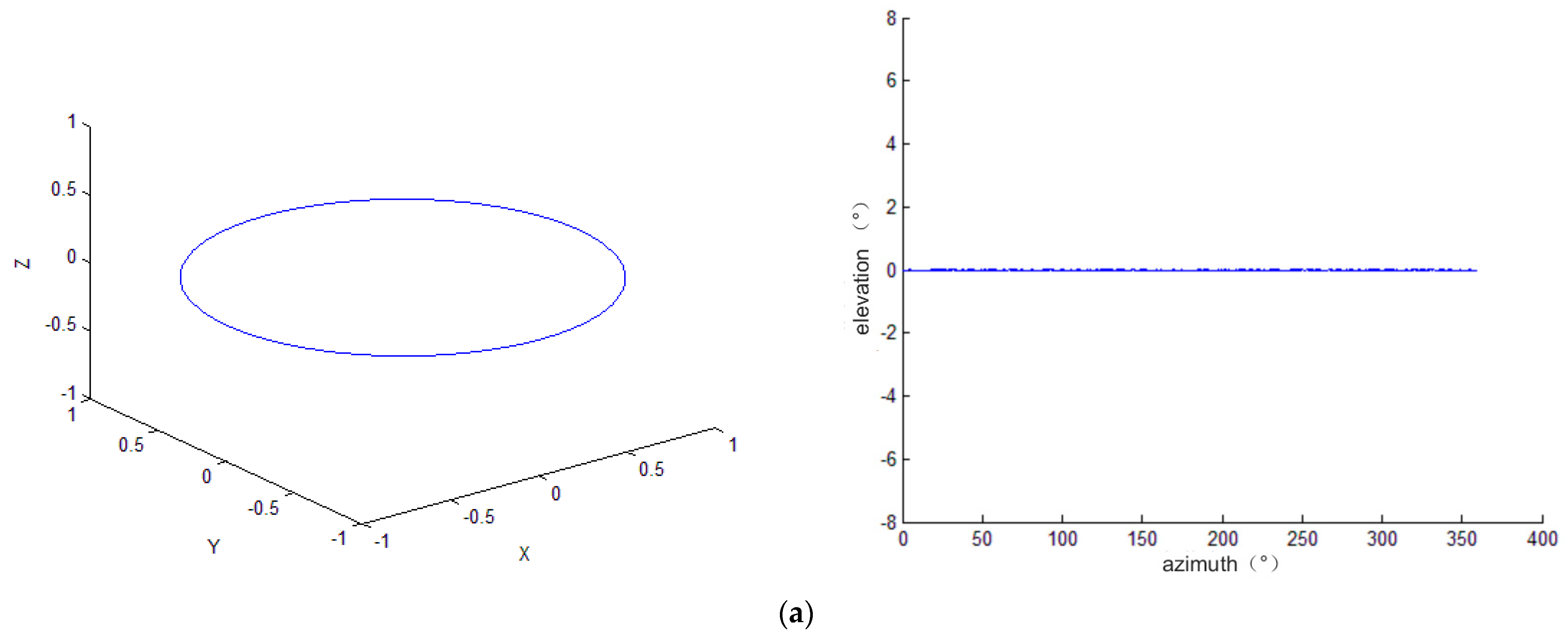
6. Experimental Results

The USV electro-optical device used in the experiment has the function of two-axis LOS stabilization and is equipped with a color TV. The resolution and the vertical field angle of the TV sensor are 768 × 576 and 6.67° × 5°, respectively. The experimental area is located in a wide sea area. Before conducting the experiment, the pitch angle of the LOS of the electro-optical equipment is established at 0°, while the azimuth angle ranges from 0° to 360°. During the circumferential scanning process, sea–sky line images are captured using the TV sensor, and the corresponding roll R and pitch P of the USV are documented at the time of each image. The angle error in the pitching direction between the LOS and the sea–sky line can be calculated by Equation (28).

$$h_i^{\prime }=\frac{n_{yi}}{N_h}\times {\omega }_y+{\Delta }_{\epsilon i}$$

(28)

As shown in Figure 7, in Equation (28), $n_{yi}$ is the number of pixels in the i-th image from the LOS to the sea–sky line in the pitching direction (positive when the sea–sky line is above the LOS, otherwise negative). $N_h$ is the vertical resolution of the TV, that is $N_h=576$. ${\omega }_y$ is the vertical view field of the TV, that is ${\omega }_y=5°$. ${\Delta }_{\epsilon i}$ is the pitch error when the electro-optical device is stably controlled. For example, in Figure 7, the measured value of $n_{yi}$ is −107 and the ${\Delta }_{\epsilon i}$ is 0.02°, according to the above parameters the $h_i^{\prime }$ can be calculated as −0.91°.

The images collected by the electro-optical device during the circumferential scanning process are shown in Figure 8. Figure 8a illustrates that at an azimuth angle of 70.28°, the center of LOS intersects with the sea–sky line and subsequently moves upwards from the sea to the sky. When the azimuth angle is 160.04° (Figure 8b), the LOS reaches the peak value of 1.076° and gradually moves downward from the sky toward the sea. At 249.94°, the LOS intersects with the sea–sky line again and then continues to move downward on the sea surface. When the azimuth angle is 339.76°, the LOS reaches the valley value of −0.9722°, and after passing the valley point, it moves from the sea to the sky in the opposite direction. The azimuth difference between the peak point and the valley point is about 180°, and that between LOS and sea–sky line intersection is about 180°. This phenomenon occurs repeatedly throughout the scanning procedure, in line with the simulation outcomes presented in Section 3.

According to the method described in Section 4, the low-precision $\alpha$ and $\beta$ values calculated by special points are 1.0133° and 0.3632°, respectively. One-hundred-and-twenty groups of data collected at 3° azimuth intervals were collected from the circumferential scanning images of the electro-optical device, including azimuth $q_i$, pitch $P_i$, roll $R_i$, and elevation error angle $h_i^{\prime }$ of the LOS. We obtained 120 groups of experimental data, and

Table 1. The 120 groups of data collected in the experiment.

Frame i	Azimuth ${\mathit{q}}_{\mathit{i}}$ (°)	Pitch ${\mathit{P}}_{\mathit{i}}$ (°)	Roll ${\mathit{R}}_{\mathit{i}}$ (°)	${\mathbf{\Delta }}_{\mathit{\epsilon }\mathit{i}}$ (°)	Pixels $\mathbf{} {\mathit{n}}_{\mathit{y}\mathit{i}}$	${\mathit{h}}_{\mathit{i}}^{\prime }$ (°)
1	0.02	−2.79	0.09	0.04	102	0.925416667
2	0.89	−1.92	1.23	0.03	90	0.81125
3	3.94	1.31	2.75	−0.03	116	0.976944444
4	6.91	2.44	1.22	0	107	0.928819444
5	9.7	2.35	−1.34	−0.05	120	0.991666667
6	12.73	−2.24	−3.46	−0.02	102	0.865416667
7	15.94	−3.27	−1.18	0.02	78	0.697083333
8	18.94	0.14	2.1	0.06	120	1.101666667
9	21.95	2.05	2.25	−0.04	164	1.383611111
10	24.66	1.98	0.71	−0.01	125	1.075069444
11	27.6	3.34	−1.51	−0.01	87	0.745208333
12	31.11	0.75	−2.28	−0.02	80	0.674444444
13	33.93	−1.07	0.16	0.02	56	0.506111111
14	36.94	1.31	2	0.04	68	0.630277778
15	39.68	2.39	1.23	−0.03	146	1.237361111
16	42.65	3.05	0.83	0.01	163	1.424930556
17	45.94	5.69	−2.06	0	42	0.364583333
18	49.01	4.91	0.3	−0.03	48	0.386666667
19	52	2.25	1.85	0	38	0.329861111
20	54.64	2.12	1.46	0	33	0.286458333
21	57.64	1.88	0.34	0	29	0.251736111
22	60.93	3.79	−2.82	0	13	0.112847222
23	63.96	4.94	−1.8	0	15	0.130208333
24	67	2.71	0.93	−0.01	10	0.076805556
25	69.71	0.9	2.42	0.01	6	0.062083333
26	72.66	1.06	1.41	0	−11	−0.095486111
27	76.07	3.91	−1.08	0.02	−14	−0.101527778
28	78.98	1.99	−2.56	0	−4	−0.034722222
29	81.95	0.08	0.62	0	−30	−0.260416667
30	84.65	2.21	1.93	0.01	−37	−0.311180556
31	87.64	2.64	1.81	0	−38	−0.329861111
32	90.93	1.47	0.61	0.01	−41	−0.345902778
33	93.93	0.29	−2.49	0.01	−55	−0.467430556
34	96.99	0.08	0.41	0	−45	−0.390625
35	99.71	0.88	1.54	0	−67	−0.581597222
36	102.69	1.17	2.03	0.03	−71	−0.586319444
37	106.04	−2.54	0.1	0	−60	−0.520833333
38	108.94	−3.59	−2.02	−0.01	−90	−0.79125
39	111.96	0.08	−2.24	0	−78	−0.677083333
40	114.64	0.47	0.33	0	−67	−0.581597222
41	117.68	0.5	2.73	−0.01	−83	−0.730486111
42	120.97	3.06	1.31	0	−115	−0.998263889
43	123.95	2.65	−1.84	−0.02	−96	−0.853333333
44	126.97	0.79	−1.84	−0.02	−106	−0.940138889
45	129.64	2.36	−1.02	−0.02	−100	−0.888055556
46	132.65	1.23	1.4	−0.01	−98	−0.860694444
47	135.94	0.17	2.02	0.01	−111	−0.953541667
48	138.95	0.77	0.19	0.01	−98	−0.840694444
49	142.02	1.1	−1.39	−0.02	−99	−0.879375
50	145	5.22	−2.34	0.01	−124	−1.066388889
51	147.67	4.39	−1.17	0.02	−107	−0.908819444
52	150.64	0.88	1.35	−0.01	−108	−0.9475
53	153.96	0.74	2.44	0.01	−123	−1.057708333
54	156.95	0.27	0.89	0	−128	−1.111111111
55	160.04	0.06	−2.05	0	−126	−1.09375
56	162.71	1.7	−2.22	0	−105	−0.911458333
57	165.65	1.93	0.37	−0.01	−112	−0.982222222
58	168.91	0.3	1.91	0.01	−113	−0.970902778
59	171.96	−2.47	1.52	−0.01	−124	−1.086388889
60	174.99	−1.14	−1.01	0	−119	−1.032986111
61	177.65	−1.07	−1.57	−0.02	−104	−0.922777778
62	180.64	0.03	−1.17	0	−108	−0.9375
63	183.93	0.08	0.55	0	−94	−0.815972222
64	186.95	0.5	1.72	0	−107	−0.928819444
65	189.98	1.23	0.41	0.01	−104	−0.892777778
66	192.68	0.93	0.91	0	−105	−0.911458333
67	195.67	2.52	0.8	0	−82	−0.711805556
68	198.94	1.84	0.78	0.01	−91	−0.779930556
69	201.93	0.57	0.66	0	−84	−0.729166667
70	204.96	1.61	0.4	0	−65	−0.564236111
71	207.67	2.72	0.02	0.01	−86	−0.736527778
72	210.7	0.18	0.6	0.03	−65	−0.534236111
73	213.93	2.47	0.16	−0.01	−62	−0.548194444
74	216.91	0.46	0.39	0	−68	−0.590277778
75	219.96	0.37	0.02	−0.02	−33	−0.306458333
76	222.71	2.64	0.51	0	−50	−0.434027778
77	225.7	3.37	−1.32	0.01	−39	−0.328541667
78	228.93	2.85	0.74	0	−47	−0.407986111
79	231.94	0.31	1.03	0.02	−33	−0.266458333
80	234.97	0.75	1.64	−0.01	−18	−0.16625
81	237.69	0.58	0.78	0.02	−21	−0.162291667
82	243.95	0.1	−1.75	0.01	−24	−0.198333333
83	246.94	−1.57	0.86	0	8	0.069444444
84	249.94	0.78	1.62	−0.02	5	0.023402778
85	252.7	0.49	1.26	0.01	9	0.088125
86	255.69	−1.07	0.32	0	32	0.277777778
87	258.96	−1.28	0.92	0	93	0.807291667
88	261.94	1.97	0.14	0.02	70	0.627638889
89	264.95	2.94	0.92	−0.01	24	0.198333333
90	267.7	0.16	0.88	0.02	27	0.254375
91	270.69	0.76	0.04	−0.02	42	0.344583333
92	273.99	−2.27	−1.27	−0.01	39	0.328541667
93	276.93	−3.41	0.09	0	144	1.25
94	279.94	−1.07	0.82	0	149	1.293402778
95	282.67	0.91	1.22	0	141	1.223958333
96	285.69	−1.45	0.23	0.02	139	1.226597222
97	288.98	1.56	−1.8	−0.01	95	0.814652778
98	291.99	0.81	0.85	0	103	0.894097222
99	294.91	2.55	1.12	0	81	0.703125
100	297.95	2.56	1.78	0	82	0.711805556
101	300.71	2.57	0.77	0	92	0.798611111
102	303.74	1.55	−1.57	0	95	0.824652778
103	306.98	1.93	−1.95	0.02	132	1.165833333
104	309.9	2.82	0.36	−0.01	131	1.127152778
105	312.91	4.57	2.68	0	135	1.171875
106	315.7	5.61	2.08	−0.02	132	1.125833333
107	318.74	4.08	0.96	0	112	0.972222222
108	322.01	4.37	−2.87	−0.01	106	0.910138889
109	325.11	4.58	−1.5	0	96	0.833333333
110	327.98	2.7	0.65	−0.01	93	0.797291667
111	330.66	0.56	2.67	0	107	0.928819444
112	333.65	1.03	2.71	0	150	1.302083333
113	336.93	3.32	−1.59	0	135	1.171875
114	340	2.31	−4.48	−0.03	109	0.916180556
115	342.92	0.96	−1.8	−0.03	89	0.742569444
116	345.67	0.3	1.36	−0.01	91	0.779930556
117	348.66	−1.28	3.89	0.01	95	0.834652778
118	351.89	1.76	1.63	0.02	120	1.061666667
119	355.04	1	−4.19	−0.02	112	0.952222222
120	357.96	−2.78	−3.8	0	89	0.772569444

shows all the experimental data.

As shown in Figure 9a, the high-precision $\alpha$ and $\beta$ values obtained using the method presented in Section 4 are 0.9533 and 0.3732, respectively. The blue star points in Figure 9b are the measured values of the elevation error angle $h_i^{\prime }$, and the red dots are the elevation error values calculated based on the calculated high-precision $\alpha$ and $\beta$ values. The calculated values exhibit good agreement with the measured values. A small part of the error measurement value deviations is too large. The nearby surge obstructs the distant sea–sky line, leading to a significant elevation angle error in the measured sea–sky line. However, this does not affect the calculation of $\alpha$ and $\beta$ values as these values with large deviations can be removed during calculation, and the number of sampling points can be increased by increasing the number of circumferential scans. Finally, the values of $\alpha$ and $\beta$ are corrected according to the perpendicularity error in Section 5. Subsequently, the electro-optical device is well stabilized near the sea–sky line, as shown in Figure 10.

7. Conclusions

The influence of the installation perpendicularity error between the base of the electro-optical device and the platform of the USV on the stability control of the LOS of the electro-optical device during the circumferential scanning process is studied. In real-world scenarios, eliminating the perpendicularity error through mechanical calibration is difficult because the platform inertial navigation axis cannot be led out. In this regard, a novel method is introduced to measure and rectify the perpendicularity error utilizing sea–sky line images. The corresponding error function of LOS caused by perpendicularity errors in the elevation direction is established. The error function is a convex function concerning the perpendicularity error and can accurately identify the error with an error precision of up to 0.01°. The simulation calculations and experimental results demonstrate that the low-frequency disturbance phenomenon of the LOS near the sea–sky line during the actual scanning process is consistent with the simulation results. By measuring the elevation error angle of the LOS from the sea–sky line and using the proposed method, the perpendicularity error can be accurately calculated and then corrected using software when performing LOS stabilization control. The electro-optical device, after error correction, can eliminate low-frequency disturbances and small high-frequency vibrations of the LOS during the circumferential scanning process, thus, greatly improving the system’s LOS stabilization accuracy and image observation effect. The suggested approach is uncomplicated and efficient, making it suitable for the routine or online calibration of the electro-optical equipment used in USV, and it has considerable engineering practicality.

References

1. Barrera, C.; Padron, I.; Luis, F.S.; Llinas, O. Trends and challenges in unmanned surface vehicles (Usv): From survey to shipping. TransNav 2021, 15, 135–142. [Google Scholar] [CrossRef]
2. Villa, J.L.; Paez, J.; Quintero, C.; Yime, E.; Cabrera, J. Design and control of an unmanned Surface vehicle for environmental monitoring applications. In Proceedings of the 2016 IEEE Colombian Conference on Robotics and Automation (CCRA), Bogota, Colombia, 29–30 September 2016; pp. 1–5. [Google Scholar]
3. Kim, M.; Joung, T.-H.; Jeong, B.; Park, H.-S. Autonomous shipping and its impact on regulations, technologies, and industries. J. Int. Marit. Saf. Environ. Affairs Ship. 2020, 4, 17–25. [Google Scholar] [CrossRef]
4. Mousazadeh, H.; Jafarbiglu, H.; Abdolmaleki, H.; Omrani, E.; Monhaseri, F.; Abdollahzadeh, M.-r.; Mohammadi-Aghdam, A.; Kiapei, A.; Salmani-Zakaria, Y.; Makhsoos, A. Developing a navigation, guidance and obstacle avoidance algorithm for an Unmanned Surface Vehicle (USV) by algorithms fusion. Ocean Eng. 2018, 159, 56–65. [Google Scholar] [CrossRef]
5. Barrera, C.; Morales, T.; Moran, R.; Caudet, E.; Marrero, R.; Cianca, A.; Alcaraz, D.; Campuzano, F.; Fernandes, C.; de Sousa, J.T.B. Expanding operational ocean-observing capabilities with gliders across the Macaronesia region. In Proceedings of the Ocean Sciences Meeting 2020, San Diego, CA, USA, 16–21 February 2020. [Google Scholar]
6. Setiawan, J.D.; Septiawan, M.A.; Ariyanto, M.; Caesarendra, W.; Munadi, M.; Alimi, S.; Sulowicz, M. Development and Performance Measurement of an Affordable Unmanned Surface Vehicle (USV). Automation 2022, 3, 27–46. [Google Scholar] [CrossRef]
7. Han, J.; Kim, J. Three-dimensional reconstruction of a marine floating structure with an unmanned surface vessel. IEEE J. Ocean. Eng. 2018, 44, 984–996. [Google Scholar] [CrossRef]
8. Balestrieri, E.; Daponte, P.; De Vito, L.; Lamonaca, F. Sensors and measurements for unmanned systems: An overview. Sensors 2021, 21, 1518. [Google Scholar] [CrossRef] [PubMed]
9. Sang, H.; You, Y.; Sun, X.; Zhou, Y.; Liu, F. The hybrid path planning algorithm based on improved A* and artificial potential field for unmanned surface vehicle formations. Ocean Eng. 2021, 223, 108709. [Google Scholar] [CrossRef]
10. Wang, H.; Fu, Z.; Zhou, J.; Fu, M.; Ruan, L. Cooperative collision avoidance for unmanned surface vehicles based on improved genetic algorithm. Ocean Eng. 2021, 222, 108612. [Google Scholar] [CrossRef]
11. Liu, T.; Pang, B.; Zhang, L.; Yang, W.; Sun, X. Sea surface object detection algorithm based on YOLO v4 fused with reverse depthwise separable convolution (RDSC) for USV. J. Mar. Sci. Eng. 2021, 9, 753. [Google Scholar] [CrossRef]
12. Zhang, W.; Gao, X.-Z.; Yang, C.-F.; Jiang, F.; Chen, Z.-Y. A object detection and tracking method for security in intelligence of unmanned surface vehicles. J. Ambient. Intell. Humaniz. Comput. 2020, 10, 1279–1291. [Google Scholar] [CrossRef]
13. Kim, J.-H.; Kim, N.; Park, Y.W.; Won, C.S. Object detection and classification based on YOLO-V5 with improved maritime dataset. J. Mar. Sci. Eng. 2022, 10, 377. [Google Scholar] [CrossRef]
14. Thombre, S.; Zhao, Z.; Ramm-Schmidt, H.; García, J.M.V.; Malkamäki, T.; Nikolskiy, S.; Hammarberg, T.; Nuortie, H.; Bhuiyan, M.Z.H.; Särkkä, S. Sensors and AI techniques for situational awareness in autonomous ships: A review. IEEE Trans. Intell. Transp. Syst. 2020, 23, 64–83. [Google Scholar] [CrossRef]
15. Cormack, D.; Schlangen, I.; Hopgood, J.R.; Clark, D.E. Joint registration and fusion of an infrared camera and scanning radar in a maritime context. IEEE Trans. Aerosp. Electr. Syst. 2019, 56, 1357–1369. [Google Scholar] [CrossRef]
16. Han, J.; Cho, Y.; Kim, J.; Kim, J.; Son, N.s.; Kim, S.Y. Autonomous collision detection and avoidance for ARAGON USV: Development and field tests. J. Field Robot. 2020, 37, 987–1002. [Google Scholar] [CrossRef]
17. Zhang, Y.; Li, Q.-Z.; Zang, F.-N. Ship detection for visual maritime surveillance from non-stationary platforms. Ocean Eng. 2017, 141, 53–63. [Google Scholar] [CrossRef]
18. Prasad, D.K.; Rajan, D.; Rachmawati, L.; Rajabally, E.; Quek, C. Video processing from electro-optical sensors for object detection and tracking in a maritime environment: A survey. IEEE Trans. Intell. Transp. Syst. 2017, 18, 1993–2016. [Google Scholar] [CrossRef]
19. Liu, H.; Zhou, X.; Liu, Q.; Ma, R.; Lu, M.; Lin, J.; Ma, M. Modeling and Simulation Analysis of Optical Axis Pointing Error of Aerial Complex Optomechanical System. In Proceedings of the 2019 International Conference on Modeling, Simulation and Big Data Analysis (MSBDA 2019), Wuhan, China, 23–24 June 2019; pp. 119–123. [Google Scholar]
20. Wu, F.; Li, S.; Zhu, H.; An, C.; Cai, J.; Du, P.; Wang, C.; Cui, X.; Yan, X. Analysis on the optical axis error of the spherical shell in the electro-optical system. Optik 2018, 168, 458–461. [Google Scholar] [CrossRef]
21. Zhang, Z.; Zhou, X.; Fan, D. Analysis, modeling and correction of pointing errors for electro-optical detection systems. Acta Aeronaut. Astronaut. Sin. 2011, 32, 2042–2054. [Google Scholar]
22. Huang, L.; Ma, W.; Huang, J. Modeling and calibration of pointing errors with alt-az telescope. New Astron. 2016, 47, 105–110. [Google Scholar] [CrossRef]
23. Zhou, X.; Liu, H.; Liu, Q.; Lin, J. Modeling and optimization of the integrated TDICCD aerial camera pointing error. Appl. Opt. 2020, 59, 8196–8204. [Google Scholar] [CrossRef]
24. Masten, M.K. Inertially stabilized platforms for optical imaging systems. IEEE Contr. Syst. Mag. 2008, 28, 47–64. [Google Scholar]
25. Tang, Q.; Yang, Q.; Wang, X.; Forbes, A.B. Pointing error compensation of electro-optical detection systems using Gaussian process regression. Int. J. Metrol. Qual. Eng. 2021, 12, 22. [Google Scholar] [CrossRef]
26. Huang, B.; Li, Z.H.; Tian, X.Z.; Yang, L.; Zhang, P.J.; Chen, B. Modeling and correction of pointing error of space-borne optical imager. Optik 2021, 247, 167998. [Google Scholar] [CrossRef]
Figure 1. The device coordinate system and the deck coordinate system.
Jmse 11 00863 g001
Figure 2. Schematic for the case of a perpendicularity error in installing the electro-optical device.
Jmse 11 00863 g002
Figure 3. Attitude relationship of each coordinate system of the electro-optical device.
Jmse 11 00863 g003
Figure 4. Comparison of LOS pointing curve for two cases under three-dimensional rectangular coordinates and two-dimensional angular coordinates. (a) The LOS Pointing curve without installation perpendicularity error (both α and β are 0°). (b) The LOS pointing curve with installation perpendicularity error ( α , β ) are (−2°, 0°), (0°, 2°), (5°, 5°).
Jmse 11 00863 g004aJmse 11 00863 g004b
Figure 5. The effect of hull roll and pitch on the elevation error Δ h curve.
Jmse 11 00863 g005
Figure 6. High-precision perpendicularity error search chart with 0.1°and 0.01°steplength.
Jmse 11 00863 g006
Figure 7. The error in the pitching direction between the LOS and the sea–sky line.
Jmse 11 00863 g007
Figure 8. The LOS deviates up and down around the sea–sky line when the electro-optical device moves during circumferential scanning.
Jmse 11 00863 g008
Figure 9. Comparison of pitch angle error measurement values and fitting calculation values between the line-of-sight and the sea–sky line.
Jmse 11 00863 g009
Figure 10. Circumferential scanning image after the electro-optical device corrects the perpendicularity error.
Jmse 11 00863 g010