Article

Numerical Study on the Water Entry of a Freely Falling Unmanned Aerial-Underwater Vehicle

1
School of Oceanography, Shanghai Jiao Tong University, Shanghai 200240, China
2
School of Naval Architecture & Ocean Civil Engineering, Shanghai Jiao Tong University, Shanghai 200240, China
3
State Key Laboratory of Ocean Engineering, Shanghai Jiao Tong University, Shanghai 200240, China
*
Authors to whom correspondence should be addressed.
J. Mar. Sci. Eng. 2023, 11(3), 552; https://doi.org/10.3390/jmse11030552
Submission received: 2 February 2023 / Revised: 25 February 2023 / Accepted: 1 March 2023 / Published: 4 March 2023
(This article belongs to the Special Issue Frontiers in Deep-Sea Equipment and Technology II)

Abstract

:
The unmanned aerial–underwater vehicle (UAUV) is a new type of vehicle that can fly in the air and cruise in water and is expected to cross the free water surface several times to perform continuous uninterrupted observation and sampling. To analyze the hydrodynamic and motion characteristics of the vehicle, the whole water-entry process of a multi-degree-of-freedom UAUV with various velocity and pitch angle was investigated through a Reynolds-averaged Navier–Stokes method. The computational domain was meshed by trimmer cells. The relative movement between the vehicle and fluid domain was simulated using moving reference frame overset mesh to delineate the interaction region around vehicle body. To reduce the computational cost, adaptive mesh refinement and adaptive time-stepping strategy were used to capture the slamming pressure accurately with reasonable computational effort. First, convergence study is considered. Simulations of the vehicle with various initial velocities and different pitch angles were performed. The variable physical properties were analyzed, and detailed results through the time-varying force and velocity were shown. Initial velocity and pitch angle are found to significantly influence hydrodynamic behavior, including the time-varying force, while thickness ratio has a great impact on added mass and pressure. The results show that higher entry velocity results in greater peak vertical force. The transverse hydrodynamic characteristics for oblique water entry of the vehicle with varies pith angle are quite different.

1. Introduction

The unmanned aerial vehicle (UAV) and the autonomous underwater vehicle (AUV) have become significant in joint multidomain marine operations, which have been widely favored by research communities. A single independent unmanned vehicle cannot satisfy the mission demand well, whereas it also is a daunting challenge to integrate various kinds of vehicles into one system properly. The unmanned aerial–underwater vehicle (UAUV) exhibits the characteristics of both the UAV and AUV, which meets demands for aerial and underwater tasks. The UAUV can fly in the air and cruise in water and is expected to cross the free water surface several times (Nicolaou [1]). The UAUV concept has been introduced as the LPL (Russian abbreviation for Flying Submarine) projects by the Soviet Union, which can navigate in either air or water (Petrov [2]). So far, UAUVs are still at the stage of prototype concept, and most work has been devoted to designing a configuration fitting for both air and water domain operations, and its irregular surface shape poses some challenges in the final manufacture. With their potential civil and military requirement, UAUVs have attracted more and more attention from researchers in recent years.
The complete motion process of the vehicle consists of three main stages: air flight, underwater navigation, and media crossing motion, including water entry and exit stages. The wing-folding machinery for the vehicle is difficult to design and manufacture. The propulsion systems should be suitable for both water-to-air and air-to-water transition (Li et al. [3]). Among the key technologies for the development of UAUVs, the techniques for air-to-water transition are quite significant, especially for fixed-wing shaped UAUVs. During the transition, fixed-wing UAUVs always undergo a sharp change in hydrodynamic force and a complicated slamming phenomenon associated with cavity formation, splash, and free surface deformation, which may cause damage to the vehicles’ components. For instance, the impact load may make UAUVs bounce on the water surface, damaging their components (Oumeraci [4]). Instability of the motion may also produce negative effects for the working conditions of the cruise. Furthermore, the hydrodynamic forces of lift and drag affect motion during the smoothing and consecutive transition from air flight to water cruise (Wei et al. [5]). To consider this aspect, the hydrodynamic characteristics of UAUVs were studied in the present work using the computational fluid dynamics (CFD) method.
The pioneer reports on the phenomenon of water impact by a rigid body were published by Von Karman [6], who gave an analytical expression for the impact force derived from the momentum theorem without considering the splash-up effect. Based on Von Karman [6], Wagner [7] derived a fair flat theoretical assumption and proposed a mathematical model that obtained satisfactory results. Based on an integro-differential equation introduced by Wagner [7], Dobrovol’skaya [8] extended the model and obtained self-similar solutions for water entry of a wedge at a constant speed. Toyama [9] presented typical solutions for asymmetrical water entry of unsymmetrical section bodies without flow separation, based on the potential flow introduced by Wagner [7]. Based on Dobrovol’skaya [8], Mei et al. [10] introduced a boundary element method (BEM). Early investigations on the problem of water entry were studied by many researchers (Vorus [11], Semenov & Iafrati [12], Xu & Wu [13], Han & Sun [14]) using potential flow and boundary elements theory, and variations in pressure distribution were also obtained. Based on the accurate surface shape of the fluid-structure coupling, Wang et al. [15] established an oblique water-entry impact model coupled with ballistic and dynamic models. However, the above methods ignore some physical properties, such as viscosity, vortex, and cavitation of the fluid.
With the rapid development of high-performance computational technology in recent years, the parallelization of computation efficiency and accuracy has increased so that complicated coupling problems are expected to be solved (Afzal, 2017 [16]). Qiu et al. [17] studied the water entry process of bodies of revolution by the CFD analysis software FLUENT with user-defined functions (UDFs) and a MIXTURE process model. Based on the Reynolds-averaged Navier–Stokes (RANS) method, Guo et al. [18] simulated the planned forced landing of a transport aircraft on the water free surface and studied the water-entry impact forces and the proper initial angle. Shi et al. [19] designed a buffer cap for an underwater vehicle and analyzed the influence of various parameters on the water-entry process. Chen et al. [20] presented a numerical study of the launching and recovery process for an autonomous underwater helicopter from a research vessel using the commercial software STAR-CCM +, showing that the optimal water-entry angle was 75°, which contributes to shape optimization. Du et al. [21] studied the influence of geometrical shapes on cavity evolution, flow fields, and vortex structure evolution during water-entry processes by using experimental and OpenFOAM platforms.
By simulating the hydrodynamics of water entry, some further applications about the vehicles have also been studied by researchers. Based on the motions and forces result by numerical simulations, identification of vehicle parameters can be done thereafter. Wu et al. [22] established the dynamic model of a freely falling UAUV immerging into the water and obtained the satisfactory trajectory using a cuckoo search (CS) optimization algorithm. Wu et al. [23] also studied the cross-domain trajectory for an aerial–aquatic coaxial eight-rotor vehicle, considering the influence of navigation error. On the other hand, some control could complete the control task of the unmanned vehicle system, without a priori knowledge or an identification process. Baldi & Roy [24] designed an autopilot framework, which needs no knowledge of the vehicle dynamics and environment messages. Embedding adaptation mechanisms in guidance law, Wang & Roy [25] proposed an adaptive vector field guidance method for UAVs, where a priori knowledge is also not required, and obtained fine results in the tests on the hardware platforms.
When a fixed-wing UAUV enters the water, the impact always induces a series of problems. This work considers the hydrodynamic problems of UAUVs using the CFD method. In contrast to the regular shapes, such as wedges, cones, and circulars mentioned above, vehicles have curvy surfaces and relatively complicated shapes, which makes the problem no longer linear. The volume of fluid (VOF) method is utilized to numerically capture the free surface profiles (Wang et al. [26]), and overset mesh technology is utilized to achieve the interaction between the background domain and the body region. This technology has an instructive significance in practical engineering applications that provides a reference in the dynamic modeling of cross-domain bodies. The present study is motivated by the need to evaluate the impact loads that may induce damage to the structure or bouncing of the falling object.

2. Materials and Methods

For freely falling bodies, it is also common to assume that the motions can be decoupled into longitudinal and lateral motions. In this study, it is speculated that the vehicle enters the water in a vertical plane, as shown in the sketch in Figure 1. It is of interest to analyze the slamming force and the motion responses of the vehicle.

2.1. Governing Equations and Turbulence Model

As the velocity of the vehicle is much lower than the acoustic speed, the compressibility of water can also be ignored. Without energy exchange, the numerical solution only follows the conservation equation of mass and continuum:
ρ t + ( ρ u i ) x i = 0
( ρ u i ) t + ( ρ u i u j ) x j = p x i + ρ ( τ i j ) x j + ρ g j
where xj are the Cartesian coordinates; ui and uj are the Cartesian components of the time-averaged velocity (i, j = 1, 2, 3), p is mean pressure, ρ is the fluid density, g denotes the body forces due to the gravitational acceleration, and τij is the viscous stress tensor belonging to a new unknown in which the equations are not closed.
To close the Reynolds stresses in the equations, the RANS has been modeled with the Shear-Stress Transport (SST) k-ω model (Menter [27]). Wilcox derived a 2-equation k-ω turbulence model for the correlation between the transport equations for 2 parameters: the turbulent kinetic energy k and the specific dissipation rate ω = ε/Cμk, which are obtained from the following transport equation:
t ( ρ k ) + x i ( ρ k u i ) = x j ( Γ k k x j ) + G k ˜ Y k
and:
t ( ρ ω ) + x i ( ρ ω u j ) = x j ( Γ ω ω x j ) + G ω ˜ Y ω + D ω
where Γk and Γω are the effective diffusivities for the SST k-ω model, respectively:
Γ k = μ + μ t σ k
Γ ω = μ + μ t σ ω
where σk and σω represent the turbulent Prandtl numbers for kinetic energy k and the specific dissipation rate ω, respectively. The turbulent viscosity μt is computed as:
μ t = ρ k ω 1 max [ 1 a * , S F 2 a 1 ω ]
σ k = 1 F 1 σ k , 1 + ( 1 F 1 ) σ k , 2
σ ω = 1 F 1 σ ω , 1 + ( 1 F 1 ) σ ω , 2
where S is the modulus of the mean rate-of-strain tensor. The term G k ˜ represents the production of turbulence kinetic energy, which is defined as:
G k ˜ = min ( G k , 10 ρ β * k ω )
To evaluate the term G k consistent with the Boussinesqu hypothsesis:
G k = μ t S 2
The term G ω is defined as:
G ω = a v t G k ˜
and D ω is defined as:
D ω = 2 ( 1 F 1 ) ρ 1 ω σ ω , 2 k x j ω x j
This turbulence model provides accurate and reliable solutions for a wide variety of flows, including adverse pressure gradient flow, effectively blending the robust and accurate formulation of the model in the far field [28]. For the fully developed turbulent flow, the higher accuracy of the k-ω model helps in predicting characteristics of the flow field and tracking streamline distribution during the whole water-entry process. More details on the closure coefficients and auxiliary relationships in the above equations were presented in previous papers by Wilcox [29,30].

2.2. Treatment of Free Surface

For multiphase analyses, the Eulerian-based VOF method developed by Hirt and Nichols [31] is applied to capture the interface in multiphase flows. This method is based on the rationale of the determination of air-water interface by calculating the volume function of the air and water phases within the grids [32]. In this work, the free surface is computed through the VOF method. The VOF formulation is set to be unsteady implicit in this study. Throughout the computational domain, air above the free surface of the calm water is selected as the gas phase, while the water is selected as the liquid phase. In the beginning step, flat wave has been selected.
To simulate the time-varying process of a vehicle submerging into the water, the overset mesh technique is used to track the motion of the vehicle region. This technique utilizes a set of Chimera embedding grids to discretize complex regions into simpler meshes [33]. The scheme is to transfer physical quantities between the multiblock mesh systems by interpolations in which the solution from one grid is linked to the solution on the embedding grids.
For free surface problems and overset mesh interaction problems, the implementation of grid refinement plays an important role in the accuracy of numerical solutions. Several arbitrarily shaped volumetric control regions were previously adopted to refine some meshes near the body surface and the free surface with a larger curvature. In order to balance accuracy and efficiency during the simulation, the AMR method, which adjusts the cell grid adaptively, is developed in the STAR-CCM+. To improve the stability and the accuracy of the results during the simulation, the adaptive mesh refinement (AMR) technology is used to increase the convergence rate and reduce calculation errors and [34]. An initial uniform mesh is generated at the beginning, and the local mesh near the specified area will be redefined adaptively in next iteration step. The accuracy error of numerical solutions is the criterion for adjusting each cell node during the iteration. In the regions with higher nonlinearity, the distribution of gird nodes will be denser to increase computational accuracy using the proposed method. In order to decrease computational burden, it will be sparser in the regions with lower nonlinearity in the meantime.
Adaptive time-stepping strategy is also used to reduce run time of the simulation and attain a specified temporal resolution. In the iteration process, this strategy first calculates local time step automatically, based on the free surface Courant-Friedrichs-Lewy (CFL) condition. Then, the global time step is obtained based on Courant number weight using the rate of change of volume fraction. This adjustment is particularly useful for cases with large variations of flow topology or large varying time scales of the physics [34].

2.3. Numerical Procedure

The motion of the body interacts with the unknowns of flow characteristics, so it should be decoupled. With the dynamic fluid body interaction (DFBI) module superposed rotation and translation motion, the motions of the vehicle can be obtained at each time step. First, the pressure and shear on each boundary are obtained through Equations (1) and (2) above, and the resultant forces and moments acting on the body surface can also be calculated by integration, according to the related kinetic parameters. At this time, the accelerations can be obtained through the governing equations of the 6 degrees of freedom (6-DOF) motion solver. Once the new position and orientation of the body are updated over time, the body surface will in turn act on the nearby fluid domain. Then, the real-time physical state of the body is computed again.
The simulations are conducted using the CFD software STAR-CCM+ (version 17.02) to numerically simulate the problem. The solution method for solving the pressure-velocity coupled equation system in multiphase flow is the SIMPLE scheme algorithm. In discretization of volume fraction and turbulent kinetic energy, 1st-order upwind is selected until the residuals converge and then are turned into 2nd-order backward Euler scheme to improve precision of the simulation. The implicit unsteady algorithm is used for velocity–pressure coupling. The same numerical scheme had been used to investigated the oblique water entry of projectiles (Song & Duan [35]). The gravity acceleration in this case is set in negative z0-direction. A robust automated prism layer meshing algorithm is also used on the vehicle surface, with two-layer all y+ wall treatment, to better capture the boundary layer.

3. Test Object and Computational Mesh

In this section, studies on the water-entry process of UAUVs is carried out. This vehicle can be carried by a supporting vessel and transit between two phases smoothly. Similar to AUVs and UAVs, UAUAVs can cruise underwater and fly in the air.

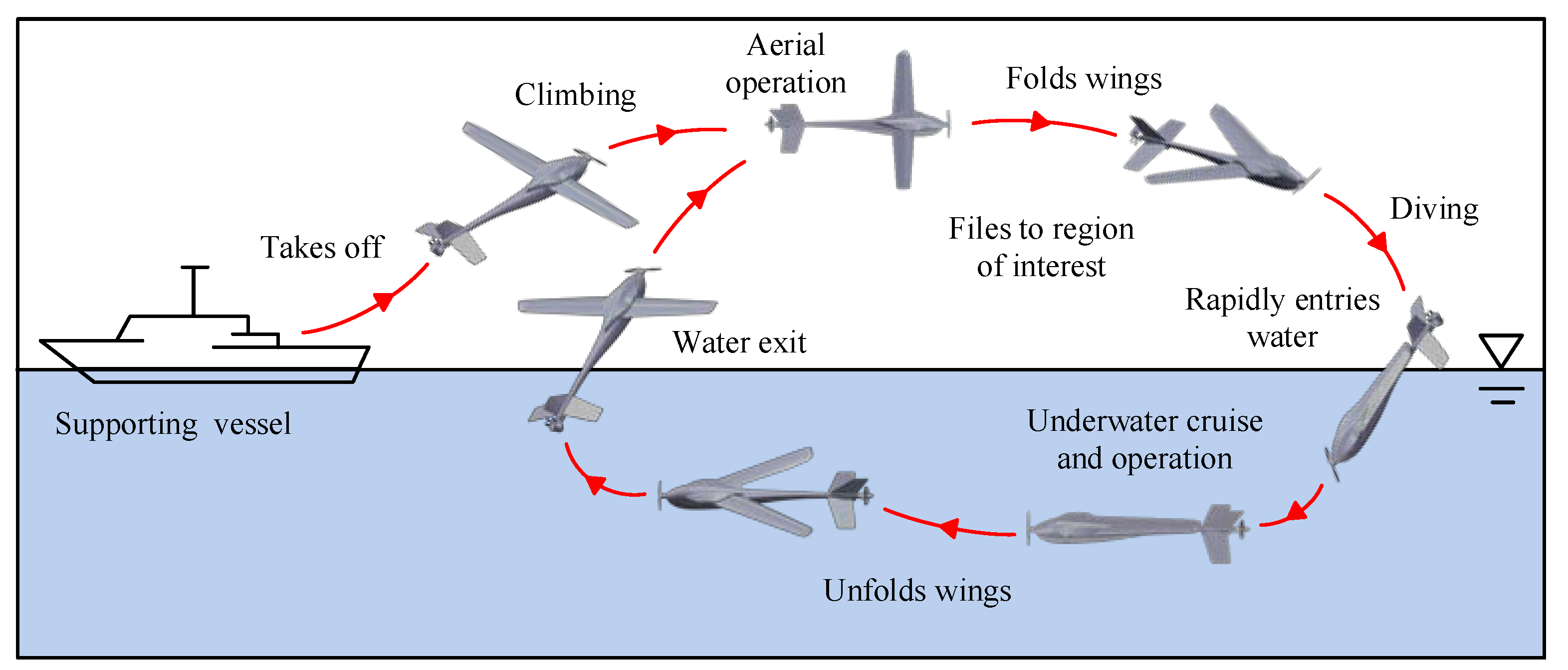
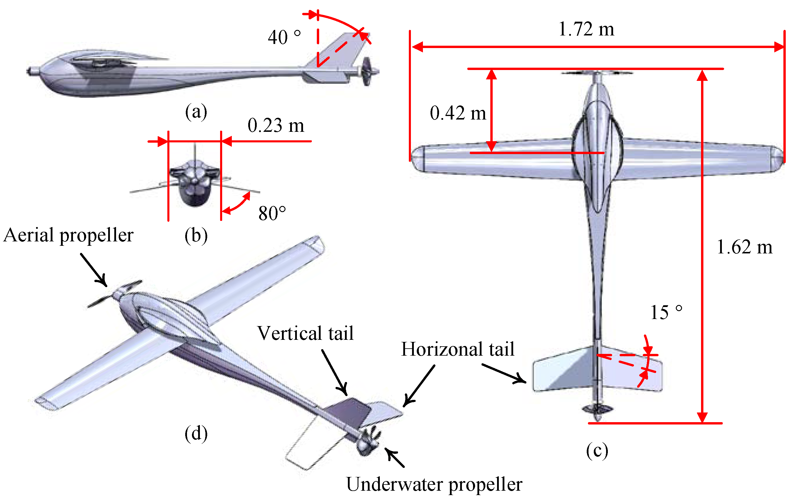
3.1. Description of the UAUV

As shown in Figure 2, the main stages of the complete operation are taking off, climbing, aerial flight, diving, water entry, underwater cruise, floating, and water exit. In an ocean survey, when the supporting vessel arrives at the ingress area, the vehicle is launched from the deck. Thereafter, the vehicle flies to the wrecked area and surveys aerially above the water surface. Then, the vehicle immerges into the water to investigate the region of interest. When the underwater cruise is completed, the vehicle floats up by the propellers. The stream flow produced by the propellers and the lift forces generated by the wings can also help the UAUV convert into flight state smoothly. Upon water exit, the UAUV communicates with the supporting vessel and transmits key data for making timely decisions afterward. Then, the UAUV could continue aerial or underwater observation missions. This vehicle has a real-time ability to exchange information and achieve extensive range of both aerial and underwater investigations such as relay communication, marine environment reconnaissance, seabed detection, and rescue applications.
Definition of the main parameters are given in Table 1, and the configuration of the UAUV is shown in Figure 3. Figure 3a–c shows three views of the UAUV and Figure 3d shows the stereogram view of the UAUV. The fixed wing is based on an ultrathin RSG-28 airfoil commonly used in UAVs, which remarkably saves space to facilitate folding. Two small winglets are implemented to improve the kinetic stability of the vehicle, ensuring aerodynamic efficiency during air flight. An aerodynamic propeller is adopted on the vehicle’s fore, and a hydrodynamic propeller is adopted on the aft.
The equilibrium of the buoyancy force and gravity influences the stability of underwater vehicles. The relative mass density of a vehicle determines its negative, positive, or neutral buoyancy. Most underwater vehicles are designed as neutrally or positively buoyant so that they can float passively in case of an accident. In the simulations, the UAUV is set as neutrally buoyant.

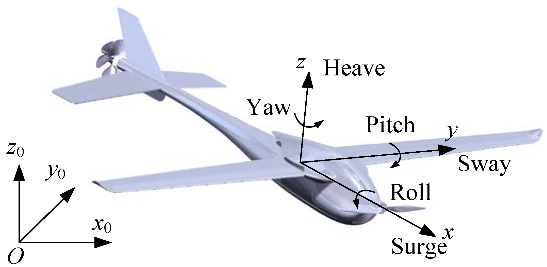
3.2. Coordinate Systems and Dimensionless Quantities

To describe the hydrodynamic forces and motions of the vehicle, there are two right-handed Cartesian coordinate systems as shown in the sketch in Figure 4. In this study, the vehicle changes its wing span and orientation before water entry, and the simulated object is the UAUV under the folded state (AUV mode). In order to display the direction of the y axis more clearly, the wings are unfolded as in Figure 4. O-x0y0z0 is the inertial Earth-fixed coordinate system, and fixed in the space is defined with O arranging at the center of gravity (CG) of the vehicle; the x0 axis coincides with the mean water surface, and the z0 axis points upward. In addition, a moving coordinate system of O-xyz fixed on the vehicle is defined, with its horizontal axis Ox and vertical axis Oz aligned at the right angle and along the moving direction of the vehicle, respectively.
To simplify the problem, the UAUV moves only in the x0-O-z0 plane and the out-of-plane motions are neglected, which indicates the motion plane of the vehicle being normal to the y0 axis. As the vehicle entered the water, the body-fixed coordinate system also moved in the x0-O-z0 plane. In this study, the simulated object is the UAUV under the folded state. The simulated forces and moments exerted on the vehicle in 3-DOF are estimated in the O-xyz coordinate including the surge force, force heave, and pitch moment, designated as X, Z and M, respectively. To simplify the problem, the aerial propeller and the underwater propeller are also neglected, because the underwater and aerial propellers will stop rotating. The water-entry process can be regarded as freely falling.

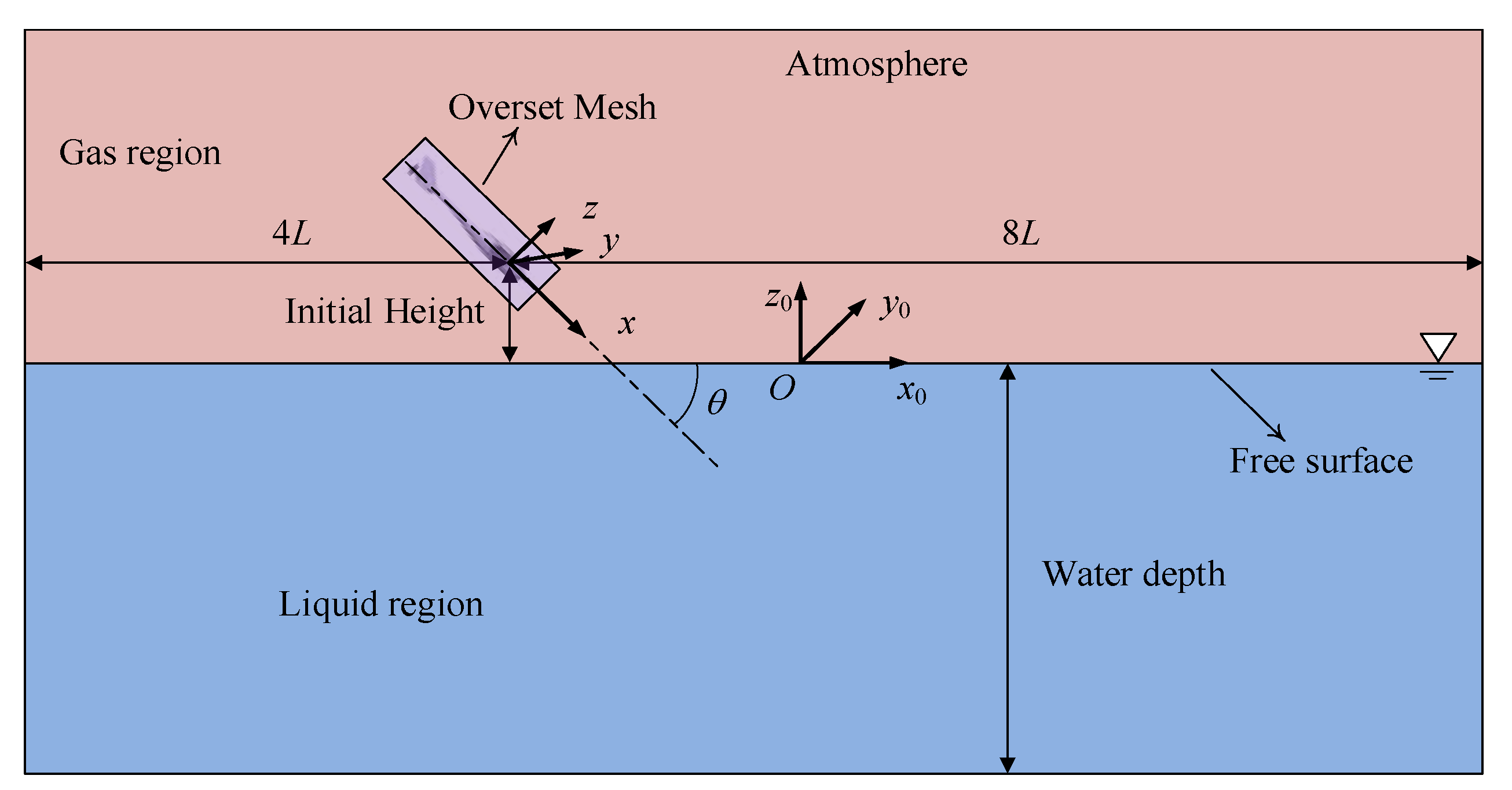
3.3. Computational Domain and Boundary Conditions

To solve the integral Equations (1) and (2) numerically, the boundaries are represented in spatial and temporal discretized form. A mesh strategy with high computational accuracy and fast efficiency should be selected for simulation calculation. The sketch of the computational domain is shown in Figure 5a. The surface remesher is used to generate the volume mesh for a trimmed nonstructured mesh, which has better geometric adaptability. There is an overset mesh block around the free surface, moving in the vertical plane, as shown in Figure 5b. Data exchange between two blocks is realized by the least square interpolation. The DFBI solver should been created, and it is necessary to specify the manner in which the vehicle body can move freely. In this study, the vehicle body is set free to translate in the x axis (lateral direction) and in the z axis (transverse direction) and to rotate about the y axis (pitch). Overset AMR and free surface AMR are utilized during the simulation process.
During the CFD simulation, a rectangular computational domain region of 12L × 10L × 5L is selected, as shown in Figure 5a. Due to the symmetry of the flow field, a symmetric surface treatment is applied for the computational domain. The vehicle surface is defined as moving walls with certain velocities. For inlet, the velocity inlet boundary is set with a specification of inlet velocity magnitude and specified at 4L upstream of the vehicle. The pressure outlet with specified pressure is specified at 8L downstream of the vehicle. After the vehicle model is released, it falls freely due to Earth’s gravity with an initial velocity. The water depth is set as 6L, and the initial height of the vehicle is specified as 0.5 m above the mean water. The y+ values should be larger than 30 to ensure accuracy for the SST k-ω model [36].

4. Convergence Study

This section describes the convergence study conducted to make sure the appropriate time step and mesh size are chosen so that the whole process of the UAUV entering the water can be solved. To test the numerical error, convergence studies were conducted for the UAUV to evaluate the influences of mesh size dl and time step Δt on the simulation results. The mesh convergence study was carried out with the dl of the fine grid to 20 mm; the dl of the other two meshes were 25.19 and 31.75 mm. The initial mesh number NT was scaled by a factor of 2.0 with three typical sizes. Therefore, three meshes were evaluated with a grid refinement ratio of rG = 2 3 , In each mesh system, the same basic length scale was applied to both background mesh and overset mesh.
Three groups of elements were chosen to carry out the grid uncertainty analysis, as shown in Table 2. The time interval of the grids changed with the decrease of mesh number due to the refinement dl. The medium grid illustrated in Figure 6a,b contains a total of 2,451,104 cells. The overset domain contains about 80% of all meshes. The cell parameters should be decided with caution, as this involves much computational resources. Meanwhile, most meshes of the background were near the free surface to obtain a convergent profile. The meshes around the block interface should be similar in size to ensure efficient data transfer through the interface. For better computational convergency, the grid size and discrete scheme should be approximate between the background and the overset region.
For a vehicle with a smooth fore, the stagnation point is near the fore and may move toward the upstream direction. According to Bernoulli’s equation, the fore of the vehicle is generally exposed to the pressure peak, which can be taken into consideration. Therefore, the maximum pressure at the fore of the vehicle is defined as a representative pressure, as shown in Figure 6b. In the simulations, the vertically deposited UAUV with initial pitch angle θ0 = 90° falls freely and vertically with Ws = 4.0 m/s, where Ws is the initial vertical water-entry velocity in the Earth-fixed coordinate. For the vertical water-entry problem, the vertical velocity W equals the transverse velocity u in the body-fixed coordinate.
The STAR-CCM+ predicted pressure at the fore and the vertical force Z0 (in z0-direction) as shown in Figure 7a,b, respectively. There are some differences between the fine mesh and the other two meshes, especially in pressure. Too coarse a mesh may cause computation divergency, because the fluid domain is discretized into unstructured trimmer cells in Star-CCM+ simulations. The basic mesh size and the time step in the third mesh could capture key features of the flow field better. However, the fine mesh system involved too much computational resources and CPU time. The hydrodynamic performance of the vehicle is one of the major focuses in present study, and the medium mesh system is enough to ensure the fidelity of hydrodynamic forces and motion during the numerical procedure, occupying fewer computational resources. Empirically based on extensive test simulation, the second mesh fits due to the compromise of computation efficiency and accuracy. The medium mesh system spatial size grid is shown in Figure 6.

5. Numerical Results and Discussions

This section computes more results of UAUVs entering the water using the present method and considers the effects of two main parameters: initial vertical velocity W and initial pitch angle θ. A series of numerical simulations are presented in this section. The initial time step Δt = 0.001 s and the basic mesh size dl = 25.19 mm are chosen for all the cases in this section. The time step and mesh are automatically adjusted during the course of calculations, followed by an adaptive time-stepping strategy and AMR technology.

5.1. Effect of Initial Vertical Velocity

This section considers four conditions in which the UAUV falls freely into the water at initial velocities of Ws = 2.0, 4.0, 8.0, and 12 m/s. According to the results, the hydrodynamic forces acting on the approximately symmetric vehicle is approximately along the vertical axis during the whole water entry, and the horizontal (in x0-direction) motion is somewhat smaller than the vertical (in z0-direction) motion. Thus, the horizontal motion can be ignored here, so this section lists only the results of the vertical motion. For the sake of comparison, the Froude number Fr can be defined as
F r = V z g L
where g is the gravity acceleration and Vz is the vertical velocity in z0-direction.
In some water-entry problems, a time-varying and deformable cavity may form while the body is immersing into the water (Birkhoff & Zarantonello [37]). To study the influence of initial velocity, the simulated free surface profiles over the UAUV at Ws = 4.0 m/s and 12.0 m/s at each moment are shown in Figure 8 and Figure 9, respectively. The deformed free surface finally tends to move downward due to the acting force from the vehicle surface and the restoring force of the gravity effect. As x position increases, the evolution of water first increases sharply and then gradually falls to zero far away from the vehicle due to the infinity boundary condition.
Figure 10a shows the jet flow around the intersection area between the water and the vehicle. The flow separation depends on the Froude number and the shape of body (Gurevich [38]). In some cases, the water would separate from the body in the absence of fluid gravity, and the water would break up into spray, as shown in Figure 10a. Streamlines around and velocity magnitude distributions at t = 0.15 s are shown in Figure 10b. Because of gravity, the fluid particles attached to the body surface were pulled down eventually, and the attached water could not be sustained indefinitely. Fluid/structure interaction may also make the flow more turbulent.
The characteristics of the predicted vertical velocity, acceleration, and hydrodynamic force are analyzed against a submergence parameter s. The depths curves of the vertical translation s and vertical velocity (in the Earth-fixed coordinate) are given in Figure 11a,b. While impacting the water, the vehicle decelerates due to the slamming force exerted on it. Through the comparison of different Ws, it was found that vertical translation varies faster with larger vertical velocity.
The velocity variation is highly correlated with the real impact velocity W0, which is the velocity magnitude when the fore end of the vehicle first touches the water. Due to the gravity effect, W0 may be larger than the intended initial speed. Table 3 shows the comparison of the velocity variation at certain positions. W1 is the velocity magnitude at s = 0.8 m, and W2 is the velocity magnitude at the final distance of s = 1.4 m. W0% = (W0 − Ws)/Ws, W1% = (W1 − Ws)/Ws, and W2% = (W2 − Ws)/Ws are the velocity variation percentages relative to Ws. Both vertical velocity reductions W1% and W2% become less for the vehicle with larger Ws. This is because in the vehicle with larger velocity the interaction of fluid/structure impact becomes more significant, thus making kinetic energy dissipate faster.
Figure 12 compares the monitored pressure at the fore of the vehicle. Undoubtedly, the pressure in the initial stage is mainly caused by the slamming, which is closely associated with the local deadrise angle (Wu et al. [39]). It can be found from the vehicle profile that the normal deadrise angle increases rapidly and then decreases gradually as the vehicle becomes submerged in water. There is a sharp peak pressure during the early stage, which can be defined as the slamming pressure. After a sharp increase, the pressure gradually decreases and then smoothly increases in the later stage. This is because the effect of fluid gravity becomes more significant in the water-entry process.
The vertical force and vertical acceleration for different initial velocities are given in Figure 13a,b. Here, the vertical force Z0 equals the transverse force in the body-fixed coordinate. As can be seen, the simulated acceleration curves from the four cases coincide with the force curves for the same case during the whole water-entry process. In addition, pressure and force with higher Ws are entirely larger than with lower Ws. Notably, the force Z0 is always positive throughout the whole water entry due to the slamming effect. This may be because more active turbulence dynamics are caused by larger induced velocity. When s is small, the local deadrise angle is smaller, thus leading to higher pressure peaks and high loads. The slamming force is normally proportional with quadratic velocity as indicated by Von Karman [6]. After the peak slamming force, the vertical hydrodynamic force decreases rapidly until it drops to the minimum positive value and then climbs up again, which can also be verified by the results of the acceleration. According to its contributing factor, the total hydrodynamic force can be divided into viscous force and pressure force. In the early water-entry stage, the pressure force occupies the main component (Xiang & Wang et al. [40]), and the hydrodynamic forces in the late stage are essentially buoyancy forces. At the same time, when Froude is low, the growth trend is faster because there is a more obvious gravity effect in the late stage.
The acceleration histories can also illustrate the trend of hydrodynamic force. In a physical meaning, when the slamming velocity decreases, the Froude number also decreases, and the influence of gravity turns into remarkable gradually. Before the vehicle touches the water, the vertical acceleration approximately equals the gravity acceleration g for the effect of freely falling. For lower Ws, the curve would not be consistent with the results of larger Ws. During the initial water-entry stage, the vertical acceleration suddenly varies to a positive peak. After the vehicle submerges, the sign of the vertical acceleration is always positive because of buoyancy, resistance, and slamming force.

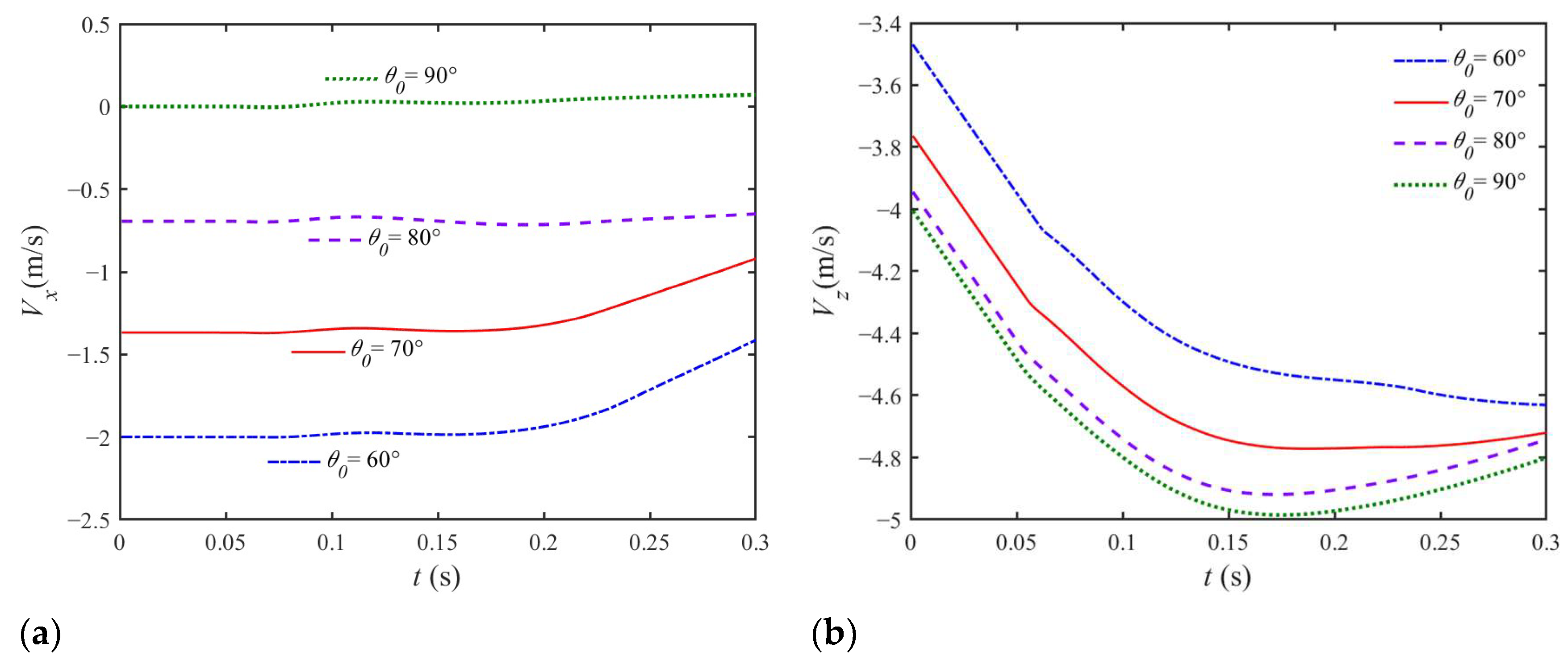
5.2. Effect of Initial Pitch Angle

Except for vertical water entry, it is of extensive interest to simulate the oblique water entry of a body with an initial pitch angle. As an important physical parameter, the difference of a vehicle’s inclination has a significant influence on the media crossing motion. The water-entry velocity is us = 4.0 m/s, and the initial pitch angles θ0 are 90° (reference case), 80°, 70°, and 60°, while holding other variables the same. The direction of initial water-entry velocity us is along the axis of the vehicle as shown in Figure 14a. Here, angle of inclination (AOI) is defined as the complementary angles of the pitch angles, which are 0°, 10°, 20°, and 30°, correspondingly. In this section, further results on horizontal motion and hydrodynamic force will be discussed.
Figure 15, Figure 16 and Figure 17 show snapshots of the free surface profiles when the UAUV enters the water with different θ0. With time, the free surface first moves upward, with the most dramatic nonlinear effect observed near the jet root with the curviest free surface. As seen in the figures, flow separation occurs more violently for the vehicle with higher horizontal velocity. It can also be found that gravity would eventually pull the water down at this velocity as discussed in Section 5.1.
Figure 18a and Figure 18b, respectively, give the time-varying moment and pitch angle of the vehicle. The net rotation of the vehicle with θ0 = 60°and 70° is much larger than the other two cases, as shown in Figure 18b. The initial pitch angle affects the horizontal translation and rotation of the vehicle as it enters the water for a longer time. A larger righting moment exerted on the vehicle accelerates its rotation and restores its orientation. Figure 19a and Figure 19b, respectively, gives the horizontal and vertical translation of the vehicle with different initial pitch angles. With time, the vehicle penetrates the water surface gradually. Transverse resistance is also exerted on the vehicle, which results in horizontal translation. The trajectories depend on both the direction of velocity and the inclination state. In Figure 19b, the curve of θ0 = 80° is close to the reference case of vertical water entry.
Figure 20 compares the time history curve of transverse and lateral forces in the body-fixed coordinate, whose direction is shown in Figure 14b. The simulated lateral force curves from all cases show similar trends, with a gentle peak in the initial stage due to the slamming effect. In the early stage of water entry, the vertical slamming peak of the transverse lateral force is sharper and slightly increases correspondingly with the increasing of inclination. Transverse force not only depends on the entry velocity but is also related to the projected wetted surface and volume. The associated wetted area of the vehicle is affected by both the pitch angle and penetration depth. When the vehicle touches the water surface, the pressure difference between the two sides results in a moment in the y0 direction, resulting in the vehicle’s rotation. As the vehicle penetrates obliquely deeper, the transverse wetted area increases, resulting in a larger drag force in the vertical direction as shown in Figure 20a. Therefore, the inclination increases due to the wetted surface area increase. Then, as result of the rotation, the associated wetted area in the horizontal direction also decreases compared with the vertical water-entry case, which causes a smaller vertical hydrodynamic force. The vertical slamming peak force slightly increases correspondingly with the increasing of inclination, and it can be inferred that vertical water entry mildly helps reduce the early vertical slamming force for a slender vehicle. As the vehicle penetrates deeper, its vertical projected wetted area constantly increases. However, for vertical water entry of θ = 90°, the curve would not be consistent with the results of oblique water entry. In the early period, the difference in vertical force become less obvious after a numerical transition period, and then the gap increases faster in a later period.
Figure 21 compares the simulated horizontal and vertical velocity history curves of the vehicle, in the O-x0y0z0 coordinate. As the vehicle enters the water for a longer time, it obviously begins moving in a transverse direction as shown in Figure 21a. It can be noticed that the final velocity at t = 0.3 s significantly decreased in contrast to us. The curve of the horizontal velocity changes less and gradually becomes close to linear. In addition, it can be clearly found in Figure 21b that the turning points of the curve are the corresponding moment when the vehicle touches the water surface. In the beginning, the lateral hydrodynamic force is still developing, so the vehicle does not move in the x0 direction. In addition, the development of transverse hydrodynamic force is not unbalanced enough. Similarly, for the water entry of the cylinder, vortex is only induced after the initial ‘warm-up’ stage (Xiang & Wang et.al [36]). As shown in Figure 15, Figure 16 and Figure 17, it can be observed that more flow separation occurs for the oblique water-entry cases in the later stage. More energy transfers to the water because of horizontal velocity, generating more water splashes. On the other hand, the pressure difference between the two sides of lager inclination is larger, resulting in a much larger horizontal hydrodynamic force. Thus, more air is trapped on the downstream side, which can also be observed in Figure 15, Figure 16 and Figure 17. Compared with the oblique water-entry cases, the time history curve of transverse force for the vertical water entry is much flatter in the later stage. In the early stage, the pitch angle has less effect on both transverse force and lateral force. Over time, the pitch angle produces more effect on the hydrodynamic force, especially transverse force. This may be induced by the asymmetric shedding vortex of the body with higher inclination angle.

6. Conclusions

In this work, the water-entry process of a multi-DOF vehicle have been simulated based on the RANS method with AMR technologies. The flow field and structural body motion are solved simultaneously using a DFBI solver. Numerical convergency with respect to mesh sizes and time step was verified, and more simulations were performed. Parametric studies have been conducted in addition to factors such as the vertical velocity and pitch angle of the UAUV. Flow separation occurs around the vehicle body, and some jet flow could be observed. The comparison of the time-varying velocity, pressure, force, and acceleration revealed that the vertical velocity exhibits a significant effect on the hydrodynamics of the vehicle. The results show that the slamming pressure and force occurred at the early stage. In the oblique water-entry cases, the velocity and force of the vehicle in each direction were analyzed deeply. It was found that the pitch angle significantly affects the motion and force in the later stage of water entry. The effect of initial inclination has been conducted in which the horizontal velocity decreases with a larger pitch angle. The influence of initial pitch angles on the horizontal force was more significant in the later stage of water entry. The numerical results indicated that the vertical hydrodynamic force was mainly affected by vertical velocity, and the contributions of pitch angle are less significant.
In the simulated oblique entry cases, some flow separation would occur near the vehicle body on the downstream side, around where cavities may occur. The studied vehicle is slender and symmetric, with its head entering the water vertically. Based on the present study, further investigations will be required with ventilation, air cavity phenomena, and initial air cushion.

Author Contributions

Conceptualization, Z.W. and L.L.; methodology, L.D. and Z.W.; software, L.D. and H.Z.; validation, L.D. and H.Z.; formal analysis, B.Y.; investigation, Z.W.; writing—original draft preparation, L.D.; writing—review and editing, L.D., Z.W and L.L.; project administration, L.L. All authors have read and agreed to the published version of the manuscript.

Funding

This research was funded by the project of the Shanghai Committee of Science and Technology, grant number 20dz1206600.

Institutional Review Board Statement

Not applicable.

Informed Consent Statement

Not applicable.

Data Availability Statement

Not applicable

Conflicts of Interest

The authors declare no conflict of interest.

References

  1. Nicolaou, S. Flying Boats & Seaplanes: A History from 1905; Bay View Books Ltd.: Bideford, UK, 1996. [Google Scholar]
  2. Petrov, G. Flying submarine. J. Fleet. 1995, 3, 52–53. [Google Scholar]
  3. Li, Y.; Feng, J.; Hu, J.; Yang, J. Research on the motion characteristics of a trans-media vehicle when entering water obliquely at low speed. Int. J. Nav. Archit. Ocean Eng. 2018, 10, 188–200. [Google Scholar] [CrossRef]
  4. Oumeraci, H. Review and analysis of vertical breakwater failures—Lessons learned. Coast. Eng. 1994, 22, 3–29. [Google Scholar] [CrossRef]
  5. Wei, Z.; Teng, Y.; Meng, X.; Yao, B.; Lian, L. Lifting-principle-based design and implementation of fixed-wing unmanned aerial–underwater vehicle. J. Field Robot. 2022, 39, 694–711. [Google Scholar] [CrossRef]
  6. Von Karman, T. The Impact on Seaplane Floats during Landing; Tech. Rep. Arch. Image Librar: Washington, DC, USA, 1929; Available online: https://digital.library.unt.edu/ark:/67531/metadc54062/ (accessed on 15 March 2019).
  7. Wagner, H. Uber Stoss—und Gleitvorgange an der oberflacke flussigkiten. ZAMM 1932, 4, 193–235. [Google Scholar] [CrossRef]
  8. Dobrovol’skaya, Z.N. On some problems of similarity flow of fluid with a free surface. J. Fluid Mech. 1969, 36, 805–829. [Google Scholar] [CrossRef]
  9. Toyama, Y. Two-dimensional water impact of unsymmetrical bodies. J. Soc. Nav. Arch. Jpn. 1993, 173, 285–291. [Google Scholar] [CrossRef]
  10. Mei, X.; Liu, Y.; Yue, D.K. On the water impact of general two-dimensional sections. Appl. Ocean Res. 1999, 21, 1–15. [Google Scholar] [CrossRef]
  11. Vorus, W.S. A flat cylinder theory for vessel impact and steady planing resistance. J. Ship Res. 1996, 40, 89–106. [Google Scholar] [CrossRef]
  12. Semenov, Y.A.; Iafrati, A. On the nonlinear water entry problem of asymmetric wedges. J. Fluid Mech. 2006, 547, 231–256. [Google Scholar] [CrossRef]
  13. Xu, G.; Wu, G.; Duan, Y. Axisymmetric liquid block impact on a solid surface. Appl. Ocean Res. 2011, 33, 366–374. [Google Scholar] [CrossRef]
  14. Han, B.; Peng, Y.; Li, H.; Liu, S.; Sun, S.; Shan, Y.; Sun, Z. Numerical investigations of a 2D bow wedge asymmetric free-falling into still water. Ocean Eng. 2022, 266, 112905. [Google Scholar] [CrossRef]
  15. Wang, Y.; Shi, X.; Wang, P. Modeling and simulation of oblique water-entry of disk Ogive. Torpedo Technol. 2008, 16, 14–17. [Google Scholar]
  16. Afzal, A.; Ansari, Z.; Faizabadi, A.R.; Ramis, M.K. Parallelization Strategies for Computational Fluid Dynamics Software: State of the Art Review. Arch. Comput. Methods Eng. 2017, 24, 337–363. [Google Scholar] [CrossRef]
  17. Qiu, H.; Yuan, X.; Wang, Y.; Liu, C. Simulation on impact load and cavity shape in high speed vertical water entry for an axisymmetric body. Torpedo Technol. 2013, 21, 161–164. [Google Scholar]
  18. Guo, B.; Liu, P.; Qu, Q.; Wang, J. Effect of pitch angle on initial stage of a transport airplane ditching. Chin. J. Aeronaut. 2013, 26, 17–26. [Google Scholar] [CrossRef] [Green Version]
  19. Shi, Y.; Pan, G.; Huang, Q. Water entry impact cushioning performance of mitigator for AUV. In Oceans 2017-Aberdeen; IEEE: Aberdeen, UK, 2017. [Google Scholar]
  20. Chen, C.; Wang, T.; Feng, Z.; Lu, Y.; Huang, H.; Ji, D.; Chen, Y. Simulation research on water-entry impact force of an autonomous underwater helicopter. J. Mar. Sci. Technol. 2020, 25, 1166–1181. [Google Scholar] [CrossRef]
  21. Du, Y.; Wang, Z.; Wang, Y.; Wang, J.; Qiu, R.; Huang, C. Study on the cavity dynamics of water entry for horizontal objects with different geometrical shapes. Ocean Eng. 2022, 252, 111242. [Google Scholar] [CrossRef]
  22. Wu, Y.; Li, L.; Su, X.; Gao, B. Dynamics modeling and trajectory optimization for unmanned aerial-aquatic vehicle diving into the water. Aerosp. Sci. Technol. 2019, 89, 220–229. [Google Scholar] [CrossRef]
  23. Wu, Y.; Li, L.; Su, X.; Cui, J. Multi-phase trajectory optimization for an aerial-aquatic vehicle considering the influence of navigation error. Eng. Appl. Artif. Intel. 2020, 89, 103404. [Google Scholar] [CrossRef]
  24. Baldi, S.; Roy, S.; Yang, S. Towards adaptive autopilots for fixed-wing unmanned aerial vehicles. In Proceedings of the 2020 59th IEEE Conference on Decision and Control (CDC), Jeju, Korea, 14–18 December 2020; IEEE: New York, NY, USA, 2020. [Google Scholar]
  25. Wang, X.; Roy, S.; Farì, S.; Baldi, S. Adaptive Vector Field Guidance Without a Priori Knowledge of Course Dynamics and Wind. IEEE/ASME Trans. Mechatron. 2022, 27, 4597–4607. [Google Scholar] [CrossRef]
  26. Wang, Z.; Stern, F. Volume-of-fluid based two-phase flow methods on structured multiblock and overset grids. Int. J. Numer. Methods Fluids 2022, 94, 557–582. [Google Scholar] [CrossRef]
  27. Menter, F.R. Two-equation eddy-viscosity turbulence models for engineering applications. AIAA J. 1994, 32, 1598–1605. [Google Scholar] [CrossRef] [Green Version]
  28. Durbin, P.A.; Reif, B.P. Statistical Theory and Modeling for Turbulent Flows; John Wiley & Sons: Chichester, West Sussex, UK, 2011. [Google Scholar]
  29. Wilcox, D.C. Turbulence Modeling for CFD; DCW Industries: La Canada, CA, USA, 1998. [Google Scholar]
  30. Wilcox, D.C. Formulation of the k-w turbulence model revisited. AIAA J. 2008, 46, 2832–2838. [Google Scholar] [CrossRef] [Green Version]
  31. Hirt, C.W.; Nichols, B.D. Volume of fluid (VOF) method for the dynamics of free boundary. J. Comput. Phys. 1981, 39, 201–225. [Google Scholar] [CrossRef]
  32. Nova Science Publishers. Multiphase Flow Research; Nova Science Publishers: New York, NY, USA, 2009. [Google Scholar]
  33. Zahle, F.; Sørensen, N.N.; Johansen, J. Wind turbine rotor-tower interaction using an incompressible overset grid method. Wind Energy Int. J. Prog. Appl. Wind Power Convers. Technol. 2009, 12, 594–619. [Google Scholar] [CrossRef]
  34. Siemens Digital Industries Software. STAR-CCM+ User Guide, Version.17.02; Siemens PLM Software: Plano, TX, USA, 2022; pp. 6882–7019. [Google Scholar]
  35. Song, Z.; Duan, W.; Xu, G.; Zhao, B. Experimental and numerical study of the water entry of projectiles at high oblique entry speed. Ocean Eng. 2020, 211, 107574. [Google Scholar] [CrossRef]
  36. Qiu, S.; Ren, H.; Li, H. Computational Model for Simulation of Lifeboat Free-Fall during Its Launching from Ship in Rough Seas. J. Mar. Sci. Eng. 2020, 8, 631. [Google Scholar] [CrossRef]
  37. Birkhoff, G.; Zarantonello, E. Jets, Wakes, and Cavities; Elsevier: New York, NY, USA, 1960; p. 261. [Google Scholar]
  38. Gurevich, M. The Theory of Jets in an Ideal Fluid; Elsevier: Amsterdam, The Netherlands, 2014. [Google Scholar]
  39. Wu, G.; Sun, H.; He, Y. Numerical simulation and experimental study of water entry of a wedge in free fall motion. J. Fluids Struct. 2004, 19, 277–289. [Google Scholar] [CrossRef]
  40. Xiang, G.; Wang, S.; Soares, C.G. Study on the motion of a freely falling horizontal cylinder into water using OpenFOAM. Ocean Eng. 2020, 196, 106811.1–106811.13. [Google Scholar] [CrossRef]
Figure 1. The sketch of the problem definition.
Jmse 11 00552 g001
Figure 2. Schematic sketch of operational regimes of the UAUV.
Jmse 11 00552 g002
Figure 3. Prototype configuration for the UAUV: (ac) three views; (d) stereogram view.
Jmse 11 00552 g003
Figure 4. Schematic diagram of the Earth-fixed coordinate and body-fixed coordinate system of the UAUV.
Jmse 11 00552 g004
Figure 5. The sketch of CFD settings: (a) configuration of the boundary conditions; (b) mesh of computational domain.
Jmse 11 00552 g005
Figure 6. The sketch of the CFD mesh generations: (a) cross-view details; (b) mesh partition of the UAUV surface.
Jmse 11 00552 g006
Figure 7. Convergent analysis of the time history curves of (a) pressure at the fore; (b) vertical force for the water entry of UAUV with different mesh systems.
Jmse 11 00552 g007
Figure 8. Free surface profiles of the vehicle entering water at Ws = 4.0 m/s at different times: (a) t = 0.10 s, (b) t = 0.15 s, (c) t = 0.20 s, (d) t = 0.25 s, and (e) t = 0.30 s.
Jmse 11 00552 g008
Figure 9. Free surface profiles of the UAUV entering water at Ws = 12.0 m/s at different times: (a) t = 0.04 s, (b) t = 0.06 s, (c) t = 0.08 s, (d) t = 0.08 s, and (e) t = 0.12 s.
Jmse 11 00552 g009
Figure 10. Profiles for (a) jet flow and (b) streamlines around the UAUV with Ws = 4.0 m/s at t = 0.15 s.
Jmse 11 00552 g010
Figure 11. Comparison of the depth curve of (a) vertical displacement and (b) vertical velocity for the water entry of UAUV with different initial velocities.
Jmse 11 00552 g011
Figure 12. Comparison of the time history curve of monitored pressure for water entry of UAUV with various initial velocities.
Jmse 11 00552 g012
Figure 13. Comparison of the displacement curve of (a) vertical force and (b) vertical acceleration for the water entry of UAUV with different initial velocities.
Jmse 11 00552 g013
Figure 14. The sketch of the CFD mesh partition of (a) initial time and (b) running time of the oblique water entry.
Jmse 11 00552 g014
Figure 15. Free surface profiles of the vehicle entering water at θ0 = 60° at different times: (a) t = 0.10 s, (b) t = 0.15 s, (c) t = 0.20 s, (d) t = 0.25 s, and (e) t = 0.30 s.
Jmse 11 00552 g015
Figure 16. Free surface profiles of the vehicle entering water at θ0 = 70° at different times: (a) t = 0.10 s, (b) t = 0.15 s, (c) t = 0.20 s, (d) t = 0.25 s, and (e) t = 0.30 s.
Jmse 11 00552 g016
Figure 17. Free surface profiles of the vehicle entering water at θ0 = 80° at different times: (a) t = 0.10 s, (b) t = 0.15 s, (c) t = 0.20 s, (d) t = 0.25 s, and (e) t = 0.30 s.
Jmse 11 00552 g017
Figure 18. Comparison of time history curve of (a) moment and (b) pitch angle for the water entry of UAUV with different initial pitch angles.
Jmse 11 00552 g018
Figure 19. Comparison of time history curve of (a) horizontal translation and (b) vertical translation for the water entry of UAUV with different initial pitch angles.
Jmse 11 00552 g019
Figure 20. Comparison of time history curve of (a) transverse force and (b) lateral force for the water entry of UAUV with different initial pitch angles.
Jmse 11 00552 g020
Figure 21. Comparison of time history curve of (a) horizontal velocity and (b) vertical velocity for the water entry of UAUV with different initial pitch angles.
Jmse 11 00552 g021
Table 1. Parameters of the object.
Main ParametersSymbolUnitQuantitative Values
Length of the vehicleLm1.62
Span of the wing (UAV moed)bm1.72
Width of the vehicle (AUV mode)Bm0.23
Weight of the vehicleWkg7.86 kg
Pitch angle of the vehicleθ°variable
Table 2. Detailed information on the initial mesh systems.
MeshBasic Mesh Size dl (mm)Time Interval Δt (s)Initial Mesh Number NT
Coarse31.750.0021225 k
Medium25.190.0012451 k
Fine200.00054902 k
Table 3. Comparison of the velocity variation of the UAUV with various Ws.
Initial VelocityW0 [m/s]W1 [m/s]W2 [m/s]W0%W1%W2%
Ws = 2.0 m/s2.8853.7663.66744.2488.28%83.37%
Ws = 4.0 m/s4.4864.9854.81412.1624.63%20.35%
Ws = 8.0 m/s8.2488.2197.7843.112.73%−2.70%
Ws = 12.0 m/s12.14811.79311.1171.24−1.73%−7.36%
Disclaimer/Publisher’s Note: The statements, opinions and data contained in all publications are solely those of the individual author(s) and contributor(s) and not of MDPI and/or the editor(s). MDPI and/or the editor(s) disclaim responsibility for any injury to people or property resulting from any ideas, methods, instructions or products referred to in the content.

