Article

Analysis of the Descent Process and Multi-Objective Optimization Design of a Benthic Lander

1
School of Mechanical Engineering, Hangzhou Dianzi University, Hangzhou 310018, China
2
Key Laboratory of Marine Biogenetic Resources, Third Institute of Oceanography, Ministry of Natural Resources, Xiamen 361005, China
*
Authors to whom correspondence should be addressed.
These authors contributed equally to this work.
J. Mar. Sci. Eng. 2023, 11(1), 224; https://doi.org/10.3390/jmse11010224
Submission received: 21 November 2022 / Revised: 6 January 2023 / Accepted: 13 January 2023 / Published: 15 January 2023
(This article belongs to the Special Issue Frontiers in Deep-Sea Equipment and Technology II)

Abstract

:
The growing need for deep-sea biological research and environmental monitoring has expanded the demand for benthic landers. Compared with remotely operated vehicles (ROVs) and autonomous underwater vehicles (AUVs), benthic landers can reduce overall operation cost and also possess longer endurance. Configuring a suitable descent velocity is important for benthic lander designs, helping them avoid retrieval failure and improve sea trial efficiencies. In this study, an effective scheme for the configuration and optimization of a self-developed benthic lander was outlined. First, the structural characteristics of the benthic lander were analyzed, and then a dynamic model was established. Second, the hydrodynamic coefficients of the benthic lander during its descent process were calculated using computational fluid dynamics (CFD) methods. Third, the MATLAB Simulink simulation environment was used to solve the dynamic model, and then the multi-objective optimization algorithm was introduced for the optimization design. Finally, the model was validated based on sea trial data, which demonstrated that the designed configuration and optimization scheme were correct and efficient. Collectively, this work provides a useful reference for the rational configuration and practical application of benthic landers.

1. Introduction

The deep sea is rich in energy, minerals and biogenetic resources; thus, it has significant economic value [1,2]. The impact of human activities on the marine environment is continually increasing [3,4], especially in offshore areas, but the response of the deep-sea to human activities remains unclear. In recent years, a large number of underwater vehicles have been used in marine climate change exploration, deep-sea observation, bioprospecting, mineral resource development and other fields. However, the mobility of conventional ROVs is severely limited due to the connection of the umbilical cable, while the cost of ROV sea trials is relatively high [5,6]. Although AUVs compensate for the abovementioned ROV shortcomings, they have poor endurance [7]. In contrast, benthic landers are playing an increasingly important role due to their relatively low cost, longer endurance and reusability.
Benthic landers have been widely utilized in in situ studies of deep-sea ecology, resources and environments. In 1975, Smith et al. designed a free vehicle respirometer (FVR) that could in situ measure the oxygen consumption of benthic communities relative to abyssal depths [8]. The other two types of benthic landers—the Autonomous Lander for Biological Experiments (ALBEX) [9,10] and the deep-sea benthic environmental observation system (Benvir) [11]—were developed for studies on deep-sea sediment community oxygen consumption. With the development of marine science and engineering technology, benthic landers can be equipped with various types of sampling modules for the collection of deep-sea seawater, sediment, microfauna and macrofauna. In 2009, the sediments incubated in the benthic lander named FLUFO [12] contained seep-associated fauna, and this study reveals the relationship between methane emissions from sediments with the seep-associated fauna. In the same year, a project called the Hadal Environment and Educational Program (HADEEP) was launched; it aimed to examine hadal biology and extend ecology research [13]. In this project, benthic landers were equipped with biological traps and seawater samplers to collect hadal samples. Thereafter, two function-similar benthic landers—a 7000-m-depth-rated lander (HaiJiao) [14] and a full-ocean-depth-rated lander—were separately produced by the Shenyang Institute of Automation of Chinese Academy of Sciences and the University of California San Diego (UCSD) [15]. Recently, Wei et al. successfully mounted their newly designed multiple in situ nucleic acid collections (MISNAC) on a benthic lander (Phoenix) to collect deep-sea microbial nucleic acid samples under in situ conditions [16]. In our previous study, a novel genus-level deep-sea bacterial species was isolated from an in situ enriched consortium collected by a benthic lander [17], and the lander used there is the prototype of the lander intended for optimization in this study. Benthic landers also have important applications in deep-sea acoustics [18], geohazards [19] and ocean-bottom seismometers (OBS) [20]. Collectively, in order to have an intuitive understanding of the background, onboard sensors and sampling modules of related landers, some typical cases of deep-sea environmental and biological studies using benthic landers are summarized in Table 1.
In recent years, the frame structure of the benthic lander has also been greatly developed. The early lander mainly comprised a tripod frame [8,9,13] was constructed around a centrally located acoustic release, similarly to the FVR lander; on top of the three legs is an aluminum plate. The BIGO [21,22] lander also has a tripod frame, but a cuboid frame is added on the top of the floatation sphere array of the lander to carry more scientific devices. The three legs make up the simplest stable structure, and the plate provides a larger contact area to avoid retrieval failure caused by excessive subsidence depth with the seafloor. Then, the three legs gradually developed into four legs [23,24,25] for higher stability, which greatly increased the ability of the lander to carry scientific devices, similarly to the RAP2 [26] lander. The four-legged Gothenburg [27] lander adopted a two-frame solution, and this was significant because it allowed for the flexibility to deploy only the inner-frame from small vessels. However, landers used for ocean-bottom seismic research usually have flat boards [28] or annular structures [20,29].
The control of descent velocity is a key concern in the design and application of benthic landers. After the benthic lander separated from the ship, its descent velocity was mainly determined by the system’s configuration [30]. When the descent velocity is too low, the efficiency of the sea trial will be reduced, and the lander may also experience uncontrolled lateral drift driven by ocean currents. Simultaneously, excessive descent velocities will also lead to a series of problems, such as lander damage or sinking too deep into the seabed sediment, which may all lead to a failure in lander retrieval. To solve these problems, Mortensen et al. [31] designed crossed wings to control the descent velocity of the lander. However, the velocity was too low, which resulted in lower efficiency and higher costs in sea trials. Jun [32] and Gang et al. [33] controlled the descent velocity by integrating a hydrofoil into the lander, but the effectiveness needs to be further verified. Therefore, achieving a more direct control scheme over the descent process is a problem that needs to be considered when designing a benthic lander.
Based on the above analysis, an effective scheme for the configuration and optimization of a self-developed benthic lander was outlined in this study. This scheme started with dynamic modelling and hydrodynamic coefficients calculation. Second, the CFD methods and multi-objective optimization algorithms were used to comprehensively study the influence mechanism of several variables on the lander’s descent velocity, including the number of floatation spheres, the mass of the weight stack and the contact area of the weight stack. Finally, the mutual restriction relationship between the lander’s descent time and subsidence depth was revealed. This study provides a useful reference for the rational configuration and practical application of a benthic lander.

2. Model Establishment of the Benthic Lander

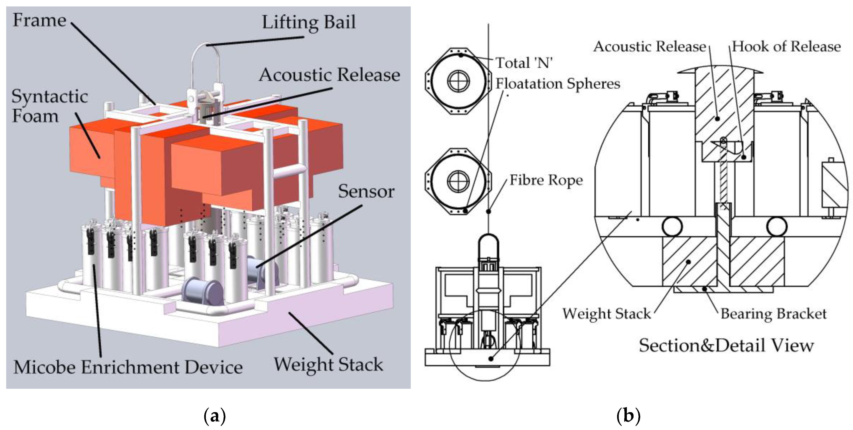
2.1. Frame Structure and Working Principle of the Benthic Lander

The lander mainly comprises three parts: an upper floatation sphere array that provides positive buoyancy, a frame that supports the scientific device and a lower weight stack that provides descending gravity (see Figure 1a). The floatation sphere array is connected in series with the fiber rope, and each floatation sphere (model: NMS-FS-6700-17RO, Nautilus Marine Service GmbH) provides 26 kg of positive buoyancy; moreover, the number of floatation spheres is configurable depending on the weight of the scientific device. The frame is made of titanium alloys. Loaded within the frame is a syntactic foam that provides positive buoyancy and structural support to the frame, and on top of the frame is a lifting bail that facilitates the process of deployment and retrieval. At the center of the frame is an acoustic release (model: OCEANO 2500S Light, iXblue, Paris, France) that is responsible for releasing the disposable weight stack. The scientific device includes the microbe enrichment device [34] array, which is the main usage of the lander, and a dual-axis inclinometer sensor (model: LCT100A, Guigangshi Lecheng Information Technology Co., Ltd., Guigang, China) with an angle resolution of 0.0001° and a 1–100 Hz configurable output frequency. The weight in water of the frame (including foam, release and science devices without the weight stack) is −85 kg, which was obtained from the water tank experiment (see Figure A1). Based on the above explanation of the lander’s frame structure, the working principle of the benthic lander is described as follows: At the end of the experiment, an acoustic remote-control unit (model: TT801, iXblue, Paris, France) is used to release the hook of the acoustic release; see Figure 1b. Then, the weight stack and bearing bracket (see Figure A2) are automatically separated from the frame, and the positive buoyancy provided by the floatation sphere array and syntactic foam allows the frame to ascend from the seafloor.

2.2. Benthic Lander Dynamic Modeling

The dynamic model of an underwater vehicle in six degrees of freedom can be described as a nonlinear equation of motion in matrix form [35]:
M υ ˙ + C υ υ + D υ υ + g η = τ
η ˙ = J η υ
where M = M R B + M A is the inertia matrix for the rigid-body mass matrix and added mass matrix, respectively;
C υ = C R B υ + C A υ is the Coriolis and centripetal matrix for rigid-body mass and added mass, respectively;
D υ = D q u a d . υ + D l i n . is the quadratic and linear damping matrix, respectively;
g η is the hydrostatic restoring force matrix resulting from the different positions of the center of buoyancy and the center of gravity;
τ is the sum of the acting forces and moments produced by the propulsion system of the vehicle, which is equal to zero in this case because the lander is a freely descending vehicle;
υ is the generalized velocity vector; accordingly, υ ˙ is the generalized acceleration vector;
η denotes the generalized position coordinates, and J is the rotation matrix for the transformation from the body-fixed frame to the earth-fixed frame. Note: M , C υ , D υ R 6 x 6 , g η , τ , υ , η R 6 x 1 .
Due to the relatively low descent velocity (please refer to the data presented in “6 Sea Trials”.), the Coriolis and centripetal matrix can be ignored, and its symmetrical structure design means that the lander is relatively stable with respect to its attitude (please refer to the data presented in “3.2. Calculation of Damping Force Coefficients”.); thus, the quadratic and linear viscous coupling coefficients between the degrees of freedom are small and can be ignored. Finally, the descent process of the next analysis was only carried out for the lander’s heave degree of freedom, and the model described in Equations (1) and (2) can be simplified as follows:
M RB + M A υ ˙ + ( D quad . υ + D lin . ) υ = g
where M RB is the mass of the lander; D quad . and D lin . are the quadratic and linear damping coefficients, respectively; υ is the descent velocity in the heave degree of freedom; −g is the net gravity for the free descending vehicle (lander). Moreover, gravity is composed of three parts: weight in seawater of the weight stack (positive), the buoyancy of the floatation sphere array (negative) and the buoyancy of the frame (negative).

3. Calculating Hydrodynamic Coefficients

3.1. Hydrodynamic Modeling

The benthic lander is an open frame structure with different configurations of the scientific device, which increases the difficulty of solving the hydrodynamic coefficients in Equation (3). The Favre-averaged Navier–Stokes (FANS) equation is a widely used method for hydrodynamic simulations of underwater vehicles with turbulent flows. In this study, the CFD software add-in, SOLIDWORKS Flow Simulation, is used to implement the FANS to compute the hydrodynamic coefficients. Assuming that the fluid comprises continuous media and does not exhibit energy conservation, the conservation laws for mass and angular momentum can be written in the conservation form as follows [36]:
ρ t + x i ρ u i = 0
ρ u i t + x j ρ u i u j + p x i = x j τ ij + τ ij R + S i   i = 1 , 2 , 3
where u is the fluid velocity, and ρ is the fluid density. Moreover, S 1 denotes a mass-distributed external force per unit mass due to a porous media resistance, and S 2 denotes buoyancy ( S 2 = ρ g i , where g i is the gravitational acceleration component along the i-th coordinate direction). S 3 denotes the coordinate system’s rotation. Moreover, τ ij denotes the viscous shear stress tensor, accordingly, τ ij R denotes the rotation form of τ ij . Significantly, with the exception of S i , other subscripts represent the corresponding coordinate direction.
The κ-ε turbulence model is used for the simulation, and the fluid volume is selected as 8 L lander × 8 W lander × 10 H lander (length, width, height (LWH)); the dimension of the lander is 0.99 × 0.97 × 1.04   m . The wall conditions and wall roughness comprise an adiabatic wall and is rated at zero, respectively. The two-scale wall functions (2SWF) model [36] was used to describe boundary layers on a fine mesh; the number of cells across a boundary layer is 8, and the corresponding approach is called the ”thick boundary layer”. To select an appropriate basic mesh size and obtain high calculation accuracy with as few cells as possible, six different basic mesh sizes were used to calculate the hydrodynamic drag force during the lander’s descent process, and the incoming flow velocity is set at 0.1 m/s and 1.0 m/s. The so-called mesh irrelevance verification is shown in Table 2.
As observed in Table 2, when the basic mesh is less than 0.09 m, the drag force gradually stabilizes and undergoes a small change. Considering limited computing resources, a basic mesh of 0.09 m is finally selected for the next CFD simulation.

3.2. Calculation of Damping Force Coefficients

In the CFD simulation, the descent velocity of the benthic lander is changed by adjusting the incoming flow velocity. The incoming flow velocity is set as 0.1–1.0 m/s, and the interval is 0.1 m/s. In contrast, Figure 2a, a cut plot, provides a contoured view of the velocity parameter distribution in which the range is divided by colored intervals; thus, each interval has its own color. Obviously, the symmetrical velocity distribution of the left and right sides also means that the damping force (D(υ)) of the lander is essentially symmetrical. Therefore, when only hydrodynamic forces are considered, the lander is relatively stable in its attitude. The damping force is a quadratic function of velocity only. From the simulated forces, the least mean square method is used to determine the hydrodynamic parameters based on Equation (3), and the results are shown in Figure 2b. The corresponding quadratic function is shown in Equation (6). As with the lander, the damping force function of a single floatation sphere is shown in Equation (7). For the full CFD data, we refer the readers to Supplementary Table S1: CFD data.
D υ = 686.5 υ 2 0.3 υ
D υ = 119.4 υ 2 + 0.5 υ

3.3. Calculation of Added Mass Coefficients
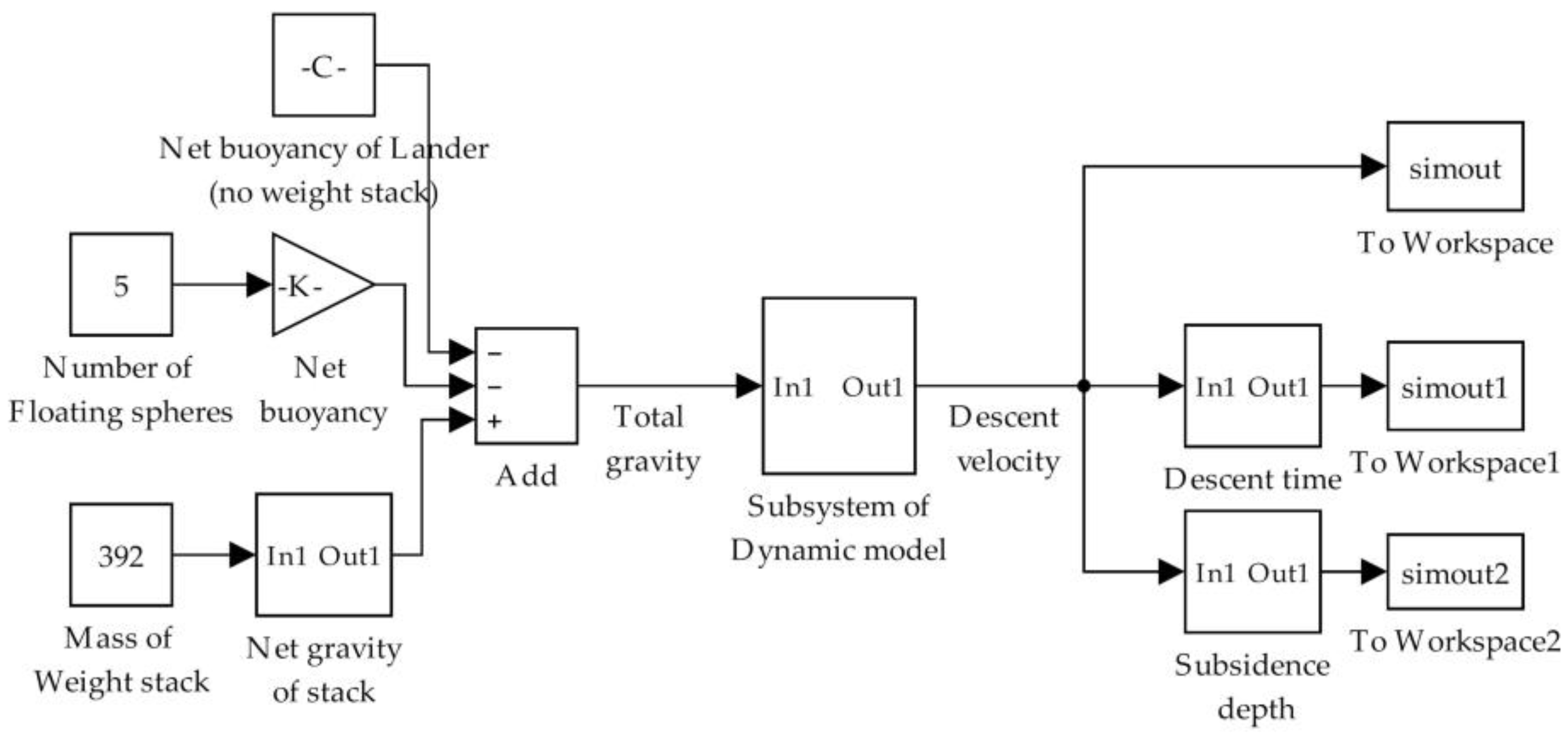
When an underwater vehicle moves in a fluid, the inertia of the fluid opposes the motion; that effect is equal to having a virtual mass added to the mass of the vehicle. In other words, when the underwater vehicle exhibits unsteady motion, it will produce added mass; we refer the reader to Equation (3). The velocities with sine functions [37] or ramp functions [38] are widely used in unsteady motions. In this study, the velocity with ramp functions was selected; we refer the reader to Equation (8), where “a” is the constant acceleration and the parameter is set as 3 groups: 0.100, 0.125 and 0.150 m / s 2 .
υ = a t
In the SOLIDWORKS Flow Simulation, the simulation project selects the time-dependent physical feature. The fluid’s unsteady motion requires a certain time period (for example, in group 3, the time approx. 13 s) to reach relatively stable acceleration velocities, and the actual acceleration is different from the set value. The actual velocity development is shown in Figure 3a, where the black dashed line represents the actual acceleration (or slope) when the steady state is attained. As shown in Equation (3), the total drag force comprises two parts: the damping force calculated in Equation (6) and the difference force generated by the added mass. The results of the explained difference force are shown in Figure 3b (in group 3, the data from groups 1 and 2 are shown in Figure A3 and Figure A4, respectively). The dashed line is the boundary at which the fluid reaches a relatively stable acceleration; obviously, the difference force is relatively constant at this boundary. Finally, bringing simulation data into Equation (3), we can obtain the added mass; we refer the reader to Table 3.

4. MATLAB Simulink

To study the influence of the lander’s configuration parameters on the variables of the descent process and based on the established dynamic model and calculated hydrodynamic coefficients, the MATLAB Simulink simulation environment was used to design the block diagram model (as we can see from Figure 4), and the corresponding file is shown in Supplementary Model S1: Simulink dynamic model. This simulation model has three input variables—the number of floatation spheres (N), the mass of the weight stack ( m stack ) and the bottom area of the weight stack ( A stack ) —and three output variables—the descent velocity ( V des ), descent time ( T des ) and subsidence depth ( D sub ) with the seafloor. The variable explanation is as follows, and the nomenclature is shown in Table 4.
  • A stack 
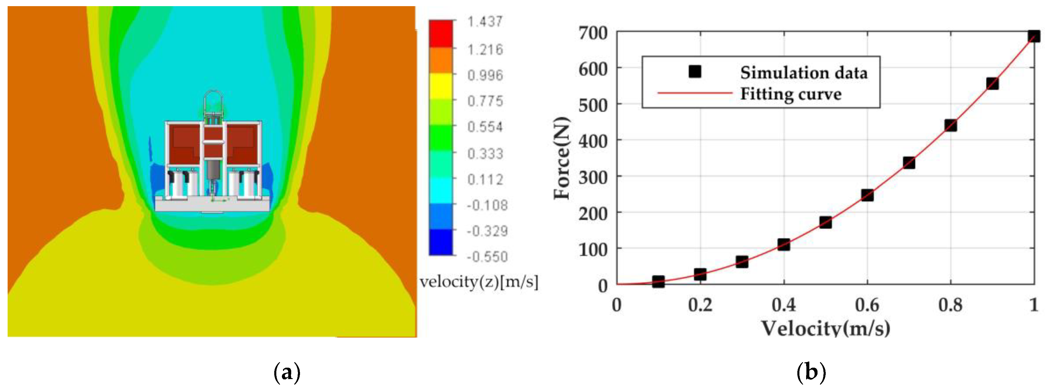
influences the hydrodynamic coefficients (as we can see from Figure A5): The corresponding function relationship is calculated by using SOLIDWORKS Flow Simulation. The results are shown in Equations (9) and (10);
  • T des takes the water depth of 5133 m during the sea trial as the background: The corresponding function is shown in Equation (11);
  • D sub was tested by a previous study [39,40] for the same benthic lander: The corresponding function is shown in Equation (12).
    D quad . = 14.29 A stack 2 23.17 A stack + 9.92
    D lin . = 14.29 A stack 2 23.17 A stack + 9.92
    T des = 5133 3600 υ
    D sub = 30.7 υ + 2.65
The dynamic model in Equation (3) is a nonlinear, first-order differential equation that may be integrated (in the Simulink diagram model, the Integrator block is used; we refer the readers to Figure A5) numerically to yield vehicle translational velocities when provided with the suitable initial conditions. The fixed-step size is 0.02 s by using the ode4 (Runge–Kutta) solver to solve the nonlinear differential equation.
Keeping the number of floatation spheres (N) constant at five in the descent process, the steady state motion was calculated by changing the mass of the weight stack ( m stack ) and the bottom area of the weight stack ( A stack ). The developmental rules of the subsidence depth ( D sub ) and descent time ( T des ) are shown in Figure 5. Obviously, the subsidence depth increases with m stack ; the smaller the bottom area, the greater m stack affects the subsidence depth. This shows that when the bottom area is small, it is easier to change the subsidence depth of the lander by adjusting m stack . In contrast, the descent time decreases with m stack ; therefore, m stack shall be appropriately increased in the sea trial in pursuit of operational efficiency.
Keeping the bottom area of the weight stack ( A stack ) constant at 0.96 m 2 in the descent process, the steady state motion was calculated by changing the mass of the weight stack ( m stack ) and the number of floatation spheres (N). The results of the descent time ( T des ) and subsidence depth ( D sub ) are shown in Figure 6. As the number of floatation spheres increases, T des increases but D sub decreases. When m stack is small, T des and D sub are more sensitive to changes in the number of floatation spheres. For example, when N is six, T des increased dramatically and lost its practical significance; thus, this situation was deleted from this Figure. Therefore, m stack should not be too small in value in order to reduce the influence of T des and D sub .

5. Multi-Objective Optimization
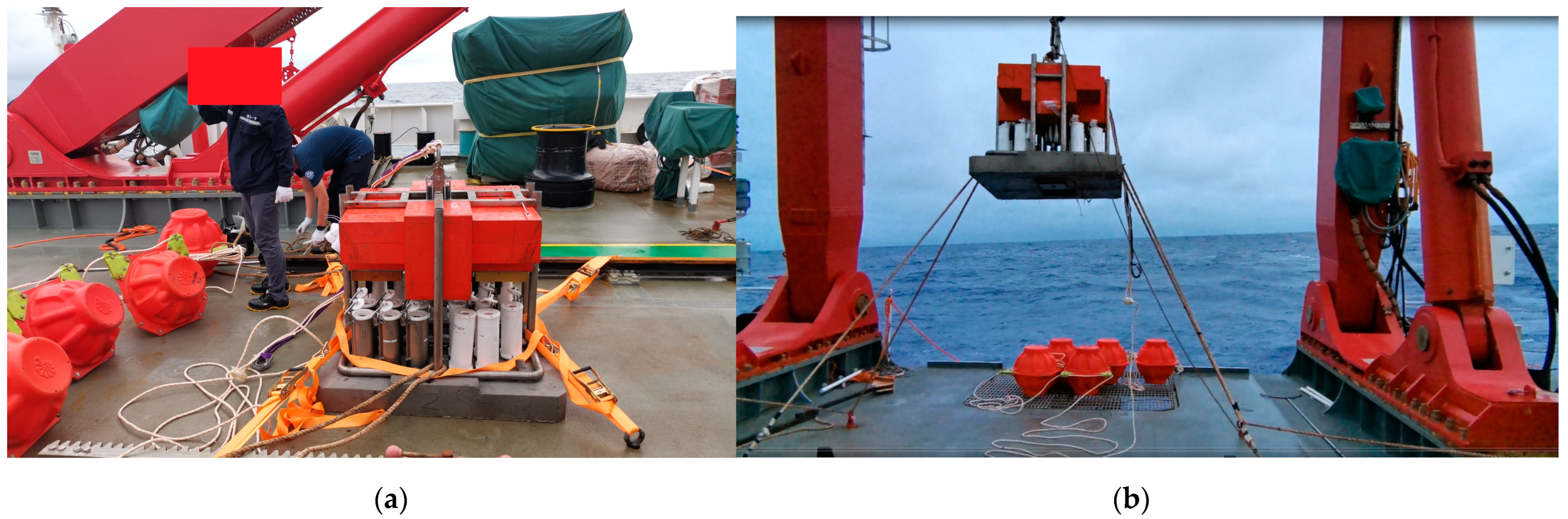
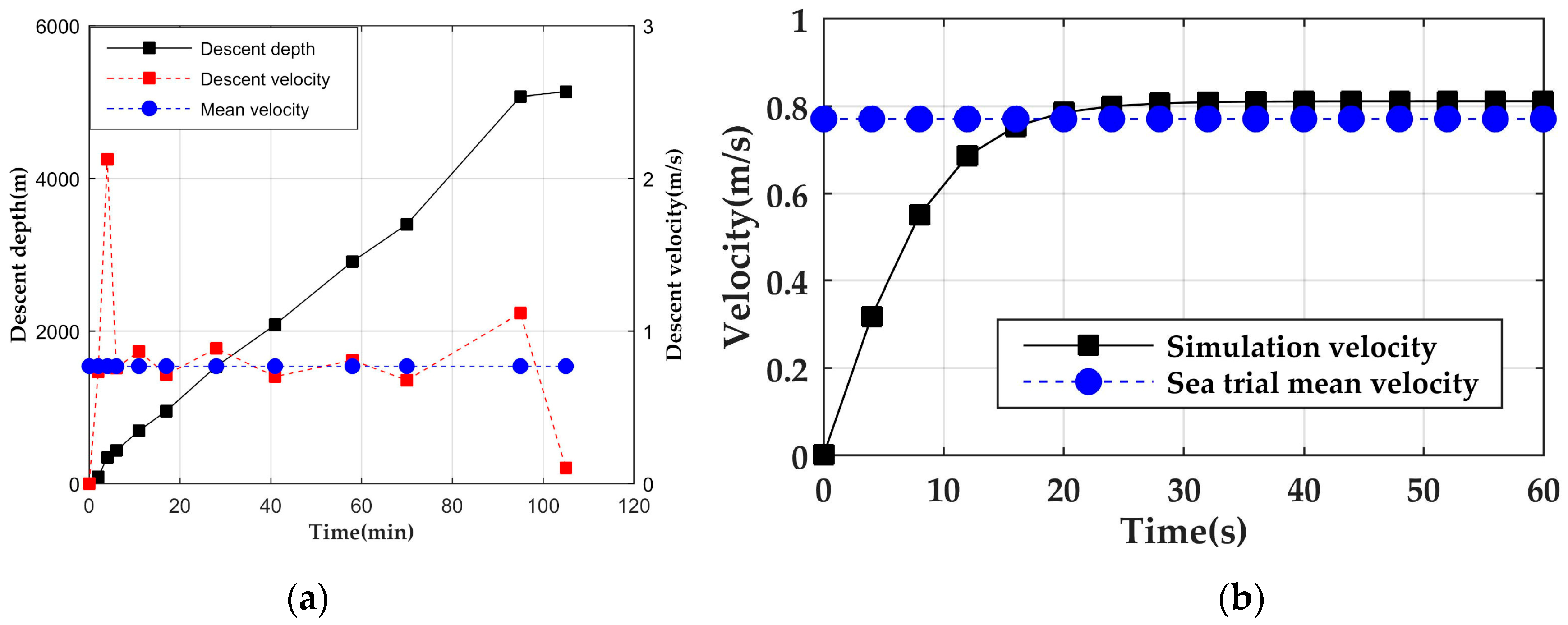
Based on the analysis of MATLAB Simulink, we know the relationship between specific configuration parameters and descent time ( T des ) and subsidence depth ( D sub ) of the lander, but making a choice is still difficult because there are various configuration schemes. Second, in practical applications, the descent time should be as small as possible to increase the operation efficiency in sea trials, and the subsidence depth should be as small as possible to avoid retrieval failure. As we can see from Figure 5, the descent time and subsidence depth are two conflicting objectives; thus, it is a multi-objective optimization problem (MOP). In this case, the objective of optimization is to minimize the descent time and subsidence depth simultaneously, which can be formulated [41] as follows:
min X F X = f 1 X , f 2 X T s . t .     g i X 0 , i = 1 , 2 , 3
where X = x 1 , x 2 , x 3 T is the decision vector; decision variable x 1 4 , 5 , 6 is the number of floatation spheres (N), which is configured by previous sea trial experience; x 2 370 580 is the mass of the weight stack ( m stack ), which is limited by the boundary of the bottom area of the weight stack ( A stack ); and x 3 0.8 1.2 is the bottom area of the weight stack ( A stack ), which is limited by the number of scientific device carried by the lander. F X is the objective vector, objective value f 1 X is the descent time ( T des ) defined in Equation (11), and f 2 X is the subsidence depth ( D sub ) defined in Equation (12). g i X denotes inequality constraints, where g 1 X ensures that the total net gravity is positive, g 2 X ensures that the descent time is less than 3 h, and g 3 X ensures that the subsidence depth is less than 45 mm. The details are described as follows, and the corresponding MATLAB code is shown in Algorithms B1.
g 1 X = 26 N 1869.7 2869.7 x 2 + 85 0
g 2 X = f 1 X 3 0
g 3 X = f 2 X 45 0
Based on the above MOP, the platform for evolutionary multi-objective optimization (PlatEMO) [42] was used to solve this problem, and the corresponding multi-objective evolutionary algorithms (MOEAs) comprise NSGA-II; [43]. The population size is set to 100, and the evaluation number is 10,000. The Pareto-optimal front (objective value) is obtained as shown in Figure 7a, and the corresponding Pareto-optimal set (decision variable) is shown in Figure 7b. The black, red and blue points distinguish the different numbers of floatation spheres. Finally, parts of the configuration from the Pareto-optimal front and set are shown in Table 5 (Supplementary Table S2: multi-objective optimization), which provides an accurate configuration reference depending on the specific T des and D sub .
The goal of MOEAs is to provide the last population with good convergence and diversity when the evaluation ends; convergence and diversity are also two important performance indicators for evaluating the optimization results. Diversity is usually measured by the diversity metric (DM) [44], and larger values are better. Convergence is usually measured by the inverted generational distance (IGD) [45], and smaller values are better. Finally, the results of the DM and IGD indicators in this study are shown in Figure 8. Obviously, the IGD tends to be stable when the number of evaluations is greater than 500; the DM has some oscillation, but the average value is approximately 0.7, both of which meet the requirements of engineering practice.

6. Sea Trials

The benthic lander sea trial was conducted in the South China Sea in July 2018 [39,40], and the newest sea trial was conducted in the western Pacific Ocean (location: 134.84°E, 16.96°N) in January 2021 (Figure 9). The corresponding video is shown in Supplementary Video S1: sea trial. The newest sea trial will be discussed in this study, and the basic configuration is N = 5, m stack = 392   kg , and A stack = 0.96   m 2 , one of the optimization results from Table 5. After the lifting device is released from the benthic lander, gravity provided by the weight stack drives the lander to freely land on the bottom of the seafloor. The original document that shows the range function of the acoustic release that obtains the relationship between the descent depth and descent time (Table 6 and Figure 10a) can be found in Supplementary Document S1: Lander deployment log sheet, and the following details are noteworthy:
  • The depth information reflected by the range data of the acoustic release is relatively accurate and reliable. First, the total mass of the lander system (603 kg) is large, and the sea current has little influence on it. Second, the successful retrieval of the lander at the original location in the later sea trials proved that the horizontal drifts during the descent process can be ignored;
  • Removal of instability during the initial launch and final landing, and the steady descent (6–70 min) velocity fluctuates between 0.68 and 0.89 m/s, which meets the expected results.
As observed in Figure 10b, the Simulink simulation velocity is basically consistent with the mean descent velocity in the sea trial; the correctness of the Simulink simulation results and CFD hydrodynamic calculation was verified; the mean descent velocity was calculated in the steady descent (6–70 min) process. As the added mass is considered in Section 2.1, the acceleration process of the lander is relatively long; at approx. 50 s, its velocity reaches the maximum and remains relatively stable. The descent time ( T des ) calculated based on the average descent velocity of the sea trial is 1.85 h. Table 5 shows that, under the sea trial configuration, the descent time obtained by using multi-objective optimizations is 1.76 h, and the relative error between the two is 5.1%. Thus, the correctness of multi-objective optimizations was verified.

7. Discussion

In this study, based on the analysis of MATLAB Simulink and CFD methods, the multi-objective optimization algorithm was used to achieve a rational configuration scheme for a benthic lander that realizes reasonable control of descent velocity. This scheme makes up the shortcomings of previous studies, for example, using crossed wings (Mortensen et al. [31]) or integrating a hydrofoil (Jun [32] and Gang et al. [33]) into the benthic lander. On the other hand, the main reasons for the higher Simulink simulation velocity (see Figure 10b) can be concluded as follows. First, the hydrodynamic drag coefficients of the lander and the floatation spheres are considered, but the coupling effects between the two are neglected. Second, the CFD damping force calculation is based on the static steady descent velocity, but the actual descent velocity has some oscillations (Figure 10a). Finally, as described in Section 6, the horizontal drifts of the lander during the descent process can be ignored, but the drifts exist, which leads to the actual descent depth being smaller than the range data from the acoustic release. However, we can conclude that the overall trend is basically correct.
In specific applications, we need to decide the descent time ( T des ) tolerated by the sea trials and the subsidence depth ( D sub ) tolerated by the lander according to Figure 7a, and the two values were used to choose a rational configuration from Table 5 (the full table see Supplementary Table S2: multi-objective optimization). Significantly, the proper number of floatation spheres (N) should be carefully selected because N has a large influence on T des and D sub (Figure 6). The population size and number of evaluations should be appropriately increased when using multi-objective optimization, which can improve the choice of configuration scheme and enhance the convergence/diversity of the population, respectively.
The results were calculated by a multi-objective optimization algorithm, and only configurations with five floatation spheres were verified in the sea trial. In future work, the number of floatation spheres at four and six still require further verification, which can comprehensively verify the correctness of the proposed scheme. The applicability of CFD simulation also needs to be tested more directly, especially since the calculation of the added mass coefficients usually has a relatively large error. In future studies, a spherical example should be introduced to test the relevant settings of SOLIDWORKS Flow Simulation in order to reduce simulation errors.

Supplementary Materials

The following supporting information can be downloaded at: https://www.mdpi.com/article/10.3390/jmse11010224/s1, Document S1: Lander deployment log sheet; Model S1: Simulink dynamic model; Table S1: CFD data; Table S2: multi-objective optimization; Video S1: sea trial.

Author Contributions

Conceptualization, D.Z. and Z.S.; methodology, D.Z. and Q.Z.; software, Q.Z.; validation, D.Z.; formal analysis, D.Z. and Q.Z.; investigation, Q.Z. and C.D.; data curation, D.Z. and C.D.; writing—original draft preparation, Q.Z. and C.D.; writing—review and editing, Q.Z., C.D., Z.S. and D.Z.; visualization, Q.Z.; supervision, D.Z. and Z.S.; project administration, D.Z. and C.D.; funding acquisition, Z.S. and D.Z. All authors have read and agreed to the published version of the manuscript.

Funding

This research was funded by the High-Tech Research and Development Program of China, grant number 2012AA092102.

Institutional Review Board Statement

Not applicable.

Informed Consent Statement

Not applicable.

Data Availability Statement

Not applicable.

Acknowledgments

We thank Gao Wei for his help with the CFD simulation and MATLAB Simulink modeling. We thank Tian Ye for his help with the multi-objective optimization. We extend our gratitude to Jianhua Xu and Dongmei Zhang for their help at sea trials. We also thank Zhao Qi for his help with the water tank experiment.

Conflicts of Interest

The authors declare no conflict of interest.

Appendix A

Figure A1. Water tank experiment.
Jmse 11 00224 g0a1
Figure A2. Bearing bracket.
Jmse 11 00224 g0a2
Figure A3. Difference force in group 1.
Jmse 11 00224 g0a3
Figure A4. Difference force in group 2.
Jmse 11 00224 g0a4
Figure A5. Subsystem of the dynamic model.
Jmse 11 00224 g0a5

Appendix B

Algorithms B1% Usage: 1.put Lander_optimization.m file to PlatEMO-1.6(can be another version)\PlatEMO\Problems\CF folder
% 2. corresponding command in matlab: main(’-algorithm’,@NSGAII,’-problem’,@Lander_optimization,’-N’,100,’-M’,2,’-D’,3,’-evaluation’,10000,’-save’,1);
% Reference: [46]
classdef Lander_optimization < PROBLEM
% <problem> <CF>
% Constrained benchmark MOP
  methods
  %% Initialization
    function obj = Lander_optimization()
     obj.Global.M = 2; %number of objects
     if isempty(obj.Global.D)
        obj.Global.D = 3; %number of decision variables
      end
      obj.Global.lower = [4370,0.8]; %lower boundary of decision variables
      obj.Global.upper = [6580,1.2]; %upper boundary of decision variables
      obj.Global.encoding = ‘real’;
    end
    %% Calculate objective values
    function PopObj = CalObj(obj,X)
      m_frame = 211; %mass of frame(without weight stack)(kg)
      G = 9.8; %gravitational acceleration(m/s2)
      Bfq = 26; %buoyancy of signal floatation sphere(kg)
      Rho_ballast = 2869.69; %the density of the ballast(kg/m3)
      Rho_water = 1000; %the density of the water(kg/m3)
      k1 = 686.5; %quadratic hydrodynamic coefficient of lander
      k2 = 119.4; %quadratic hydrodynamic coefficient of signal floatation sphere
      %round function is to towards nearest integer for the numbers of floatation sphere
      k = k2*round(X(:,1)) + k1.*(14.29.*X(:,3).^2 − 23.17.*X(:,3) + 9.92);
      %85 is the net gravity of lander without the weight stack
      g = (−Bfq.*round(X(:,1)) + X(:,2)./Rho_ballast.*(Rho_ballast-Rho_water) −85).*G./(m_frame+X(:,2));
      v = sqrt((m_frame+X(:,2)) .*g./k); %descent velocity
      PopObj(:,1) = 5133./(3600.*v); %descent time
      PopObj(:,2) = 30.7.*v + 2.65; %subsidence depth
    end
    %% Calculate constraint violations
    function PopCon = CalCon(obj,X)
      PopObj = obj.CalObj(X);
      %g_1(X) is to make sure the total net gravity is positive
      PopCon(:,1) = 26.*round(X(:,1)) − X(:,2)./2869.69.*(2869.69−1000) + 85;
      %g_2(X) is to make sure the descent time less than 3 h
      PopCon(:,2) = PopObj(:,1) − 3;
      %g_3(X) is to make sure the subsidence depth less than 45 mm
      PopCon(:,3) = PopObj(:,2) − 45;
    end
    %% Sample reference points on Pareto front
    function P = PF(obj,N)
      P(:,1) = (0.33:1/20:3)’; %the values of f1(x)
      P(:,2) = (30.7*5)./(9.*P(:,1)) + 2.65; %the values of f2(x)
    end
  end
end

References

  1. Marshall, N.B. Glimpses into Deep-Sea Biology. In The Arctic Ocean: The Hydrographic Environment and the Fate of Pollutants; Rey, L., Ed.; Palgrave Macmillan: London, UK, 1982; pp. 263–271. [Google Scholar]
  2. McLellan, B.C. Sustainability Assessment of Deep Ocean Resources. Procedia Environ. Sci. 2015, 28, 502–508. [Google Scholar] [CrossRef] [Green Version]
  3. Harrould-Kolieb, E.R.; Herr, D. Ocean Acidification and Climate Change: Synergies and Challenges of Addressing Both under the UNFCCC. Clim. Policy 2012, 12, 378–389. [Google Scholar] [CrossRef]
  4. Cooley, S.R.; Bello, B.; Bodansky, D.; Mansell, A.; Merkl, A.; Purvis, N.; Ruffo, S.; Taraska, G.; Zivian, A.; Leonard, G.H. Overlooked Ocean Strategies to Address Climate Change. Glob. Environ. Chang. 2019, 59, 101968. [Google Scholar] [CrossRef]
  5. Nunoura, T.; Takaki, Y.; Hirai, M.; Shimamura, S.; Makabe, A.; Koide, O.; Kikuchi, T.; Miyazaki, J.; Koba, K.; Yoshida, N.; et al. Hadal Biosphere: Insight into the Microbial Ecosystem in the Deepest Ocean on Earth. Proc. Natl. Acad. Sci. USA 2015, 112, E1230–E1236. [Google Scholar] [CrossRef] [Green Version]
  6. Bowen, A.D.; Yoerger, D.R.; Taylor, C.; McCabe, R.; Howland, J.; Gomez-Ibanez, D.; Kinsey, J.C.; Heintz, M.; McDonald, G.; Peters, D.B.; et al. The Nereus Hybrid Underwater Robotic Vehicle for Global Ocean Science Operations to 11,000 m Depth. In Proceedings of the OCEANS 2008, Quebec, QC, Canada, 15–18 September 2008; pp. 1–10. [Google Scholar] [CrossRef]
  7. Wynn, R.B.; Huvenne, V.A.I.; Le Bas, T.P.; Murton, B.J.; Connelly, D.P.; Bett, B.J.; Ruhl, H.A.; Morris, K.J.; Peakall, J.; Parsons, D.R.; et al. Autonomous Underwater Vehicles (AUVs): Their Past, Present and Future Contributions to the Advancement of Marine Geoscience. Mar. Geol. 2014, 352, 451–468. [Google Scholar] [CrossRef] [Green Version]
  8. Smith, K.L., Jr.; Clifford, C.H.; Eliason, A.H.; Walden, B.; Rowe, G.T.; Teal, J.M. A Free Vehicle for Measuring Benthic Community Metabolism1. Limnol. Oceanogr. 1976, 21, 164–170. [Google Scholar] [CrossRef]
  9. Duineveld, G.C.A.; Lavaleye, M.S.S.; Berghuis, E.M. Particle Flux and Food Supply to a Seamount Cold-Water Coral Community (Galicia Bank, NW Spain). Mar. Ecol. Prog. Ser. 2004, 277, 13–23. [Google Scholar] [CrossRef]
  10. Lavaleye, M.; Duineveld, G.; Lundälv, T.; White, M.; Guihen, D.; Kiriakoulakis, K.; Wolff, G. Cold-Water Corals on the Tisler Reef: Preliminary Observations on the Dynamic Reef Environment. Oceanography 2009, 22, 76–84. [Google Scholar] [CrossRef] [Green Version]
  11. Zhao, G.; Yu, X.; Li, X. Benvir: A in Situ Deep-Sea Observation for Benthic Environmental Monitoring. High Technol. Lett. 2015, 25, 54–60. [Google Scholar]
  12. Linke, P.; Sommer, S.; Rovelli, L.; McGinnis, D.F. Physical Limitations of Dissolved Methane Fluxes: The Role of Bottom-Boundary Layer Processes. Mar. Geol. 2010, 272, 209–222. [Google Scholar] [CrossRef]
  13. Jamieson, A.J.; Fujii, T.; Solan, M.; Priede, I.G. HADEEP: Free-Falling Landers to the Deepest Places on Earth. Mar. Technol. Soc. J. 2009, 43, 151–160. [Google Scholar] [CrossRef]
  14. Chen, J.; Zhang, Q.; Zhang, A.; Tang, Y. 7000M Lander Design for Hadal Research. In Proceedings of the 2014 Oceans—St. John’s, St. John’s, NL, Canada, 14–19 September 2014; pp. 1–4. [Google Scholar]
  15. Peoples, L.M.; Norenberg, M.; Price, D.; McGoldrick, M.; Novotny, M.; Bochdansky, A.; Bartlett, D.H. A Full-Ocean-Depth Rated Modular Lander and Pressure-Retaining Sampler Capable of Collecting Hadal-Endemic Microbes under in Situ Conditions. Deep. Sea Res. Part I Oceanogr. Res. Pap. 2019, 143, 50–57. [Google Scholar] [CrossRef]
  16. Wei, Z.-F.; Li, W.-L.; Li, J.; Chen, J.; Xin, Y.-Z.; He, L.-S.; Wang, Y. Multiple in Situ Nucleic Acid Collections (MISNAC) from Deep-Sea Waters. Front. Mar. Sci. 2020, 7. [Google Scholar] [CrossRef] [Green Version]
  17. Dong, C.; Ma, T.; Liu, R.; Lai, Q.; Shao, Z. Hydrocarboniclastica marina gen. nov., sp. nov., a Marine Hydrocarbonoclastic Bacterium Isolated from an in Situ Enriched Hydrocarbon-Degrading Consortium in Sea Sediment. Int. J. Syst. Evol. Microbiol. 2019, 69, 2250–2257. [Google Scholar] [CrossRef] [PubMed]
  18. Barclay, D.R.; Simonet, F.; Buckingham, M.J. Deep Sound: A Free-Falling Sensor Platform for Depth-Profiling Ambient Noise in the Deep Ocean. Mar. Technol. Soc. J. 2009, 43, 144–150. [Google Scholar] [CrossRef] [Green Version]
  19. Yonggang, J.; Chaoqi, Z.; Liping, L.; Dong, W. Marine Geohazards: Review and Future Perspective. Acta Geol. Sin.—Engl. Ed. 2016, 90, 1455–1470. [Google Scholar] [CrossRef]
  20. Montagner, J.-P.; Karczewski, J.-F.; Romanowicz, B.; Bouaricha, S.; Lognonné, P.; Roult, G.; Stutzmann, E.; Thirot, J.-L.; Brion, J.; Dole, B.; et al. The French Pilot Experiment OFM-SISMOBS: First Scientific Results on Noise Level and Event Detection. Phys. Earth Planet. Inter. 1994, 84, 321–336. [Google Scholar] [CrossRef]
  21. Sommer, S.; Pfannkuche, O.; Linke, P.; Luff, R.; Greinert, J.; Drews, M.; Gubsch, S.; Pieper, M.; Poser, M.; Viergutz, T. Efficiency of the Benthic Filter: Biological Control of the Emission of Dissolved Methane from Sediments Containing Shallow Gas Hydrates at Hydrate Ridge. Glob. Biogeochem. Cycles 2006, 20. [Google Scholar] [CrossRef] [Green Version]
  22. Sommer, S.; Linke, P.; Pfannkuche, O.; Schleicher, T.; Deimling, J.S.V.; Reitz, A.; Haeckel, M.; Flögel, S.; Hensen, C. Seabed Methane Emissions and the Habitat of Frenulate Tubeworms on the Captain Arutyunov Mud Volcano (Gulf of Cadiz). Mar. Ecol. Prog. Ser. 2009, 382, 69–86. [Google Scholar] [CrossRef]
  23. Linke, P.; Suess, E.; Torres, M.; Martens, V.; Rugh, W.D.; Ziebis, W.; Kulm, L.D. In Situ Measurement of Fluid Flow from Cold Seeps at Active Continental Margins. Deep. Sea Res. Part I Oceanogr. Res. Pap. 1994, 41, 721–739. [Google Scholar] [CrossRef]
  24. Smith, K.L.; Baldwin, R.J.; Karl, D.M.; Boetius, A. Benthic Community Responses to Pulses in Pelagic Food Supply: North Pacific Subtropical Gyre. Deep. Sea Res. Part I Oceanogr. Res. Pap. 2002, 49, 971–990. [Google Scholar] [CrossRef]
  25. Ekeroth, N.; Kononets, M.; Walve, J.; Blomqvist, S.; Hall, P.O.J. Effects of Oxygen on Recycling of Biogenic Elements from Sediments of a Stratified Coastal Baltic Sea Basin. J. Mar. Syst. 2016, 154, 206–219. [Google Scholar] [CrossRef]
  26. Khripounoff, A.; Caprais, J.-C.; Crassous, P.; Etoubleau, J. Geochemical and Biological Recovery of the Disturbed Seafloor in Polymetallic Nodule Fields of the Clipperton-Clarion Fracture Zone (CCFZ) at 5000-m Depth. Limnol. Oceanogr. 2006, 51, 2033–2041. [Google Scholar] [CrossRef] [Green Version]
  27. Kononets, M.; Tengberg, A.; Nilsson, M.; Ekeroth, N.; Hylén, A.; Robertson, E.K.; van de Velde, S.; Bonaglia, S.; Rüt-ting, T.; Blomqvist, S.; et al. In Situ Incubations with the Gothenburg Benthic Chamber Landers: Applications and Quality Control. J. Mar. Syst. 2021, 214, 103475. [Google Scholar] [CrossRef]
  28. Tréhu, A.M.; de Moor, A.; Madrid, J.M.; Sáez, M.; Chadwell, C.D.; Ortega-Culaciati, F.; Ruiz, J.; Ruiz, S.; Tryon, M.D. Post-Seismic Response of the Outer Accretionary Prism after the 2010 Maule Earthquake, Chile. Geosphere 2019, 16, 13–32. [Google Scholar] [CrossRef] [Green Version]
  29. Person, R.; Aoustin, Y.; Blandin, J.; Marvaldi, J.; Rolin, J.F. From Bottom Landers to Observatory Networks. Ann. Geophys. 2006, 49. [Google Scholar] [CrossRef]
  30. Spagnoli, F.; Penna, P.; Giuliani, G.; Masini, L.; Martinotti, V. The AMERIGO Lander and the Automatic Benthic Chamber (CBA): Two New Instruments to Measure Benthic Fluxes of Dissolved Chemical Species. Sensors 2019, 19, 2632. [Google Scholar] [CrossRef] [Green Version]
  31. Mortensen, A.C.; Lange, R.E. Design Considerations of Wing Stabilized Free-Fall Vehicles. Deep. Sea Res. Oceanogr. Abstr. 1976, 23, 1231–1240. [Google Scholar] [CrossRef]
  32. Jun, C. Research on Techniques of Hadal Lander and Applications on Biology. Ph.D. Thesis, University of Chinese Academy of Sciences, Beijing, China, 2018. [Google Scholar]
  33. Gang, X.; Yanjun, L.; Yifan, X. Hydrodynamic Characteristics Research and Structure Optimization of Hadal Lander with Hydrofoil. J. Mech. Eng. 2022, 58, 1–15. [Google Scholar]
  34. Yuanyuan, S.; Donghui, Z. Design of a Deep-Sea Microbe Enrichment Device. J. Hangzhou Dianzi Univ. 2017, 37, 57–60. [Google Scholar]
  35. Thor, I.F. Guidance and Control of Ocean Vehicles, Chapter 4; John Wiley and Sons Ltd.: New York, NY, USA, 1994. [Google Scholar]
  36. SOLIDWORKS Flow Simulation. Flow Simulation 2017 Technical Reference; Dassault System: Vélizy-Villacoublay, France, 2017. [Google Scholar]
  37. Kim, H.; Akimoto, H.; Islam, H. Estimation of the Hydrodynamic Derivatives by RaNS Simulation of Planar Motion Mechanism Test. Ocean. Eng. 2015, 108, 129–139. [Google Scholar] [CrossRef]
  38. Lack, S.; Rentzow, E.; Jeinsch, T. Experimental Parameter Identification for an Open-Frame ROV: Comparison of Towing Tank Tests and Open Water Self-Propelled Tests. IFAC-PapersOnLine 2019, 52, 271–276. [Google Scholar] [CrossRef]
  39. Yu, W. Dynamic Analysis of Sediment Sediment Bottom Sitting Process of Deep Sea Lander. Master’s Thesis, Hangzhou Dianzi University, Hangzhou, China, 2020. [Google Scholar]
  40. Yu, Z.; Zhang, C.; Chen, J.; Ren, Z. Dynamic Analysis of Bottom Subsidence of Benthic Lander. J. Mar. Sci. Eng. 2022, 10, 824. [Google Scholar] [CrossRef]
  41. Release PlatEMO v1.6 (2018/9/9), BIMK/PlatEMO, GitHub. Available online: https://github.com/BIMK/PlatEMO/releases/tag/v1.6 (accessed on 20 November 2022).
  42. Tian, Y.; Cheng, R.; Zhang, X.; Jin, Y. PlatEMO: A MATLAB Platform for Evolutionary Multi-Objective Optimization [Educational Forum]. IEEE Comput. Intell. Mag. 2017, 12, 73–87. [Google Scholar] [CrossRef] [Green Version]
  43. Deb, K.; Pratap, A.; Agarwal, S.; Meyarivan, T. A Fast and Elitist Multiobjective Genetic Algorithm: NSGA-II. IEEE Trans. Evol. Comput. 2002, 6, 182–197. [Google Scholar] [CrossRef] [Green Version]
  44. Deb, K.; Jain, S. Running Performance Metrics for Evolutionary Multi-Objective Optimizations. In Proceedings of the Fourth Asia-Pacific Conference on Simulated Evolution and Learning (SEAL’02), Orchid Country Club, Singapore, 18–22 November 2002; pp. 1–18. [Google Scholar]
  45. Coello, C.A.C.; Cortés, N.C. Solving Multiobjective Optimization Problems Using an Artificial Immune System. Genet. Program. Evolvable Mach. 2005, 6, 163–190. [Google Scholar] [CrossRef]
  46. Zhang, Q.; Zhou, A.; Zhao, S.; Suganthan, P.; Liu, W.; Tiwari, S. Multiob-jective optimization test instances for the CEC 2009 special session and competition University of Essex, Colchester, UK and Nanyang technological University, Singapore, special session on performance assessment of multi-objective optimization algorithms. Tech. Rep. 2008, 264, 1–30. Available online: https://www.researchgate.net/publication/265432807 (accessed on 20 November 2022).
Figure 1. (a) The overall structure of the benthic lander; (b) the working principle of the benthic lander.
Jmse 11 00224 g001
Figure 2. (a) Cut plot when the incoming flow velocity is 1 m/s; (b) damping force quadratic function curve of the lander.
Jmse 11 00224 g002
Figure 3. (a) The actual velocity development; (b) the difference force generated by the added mass in group 3.
Jmse 11 00224 g003
Figure 4. Simulink block diagram model.
Jmse 11 00224 g004
Figure 5. (a) Subsidence depth vs. the mass of the weight stack and bottom area of the weight stack; (b) descent time vs. mass of the weight stack and bottom area of the weight stack.
Jmse 11 00224 g005
Figure 6. Subsidence depth, descent time vs. mass of the weight stack and number of floatation spheres.
Jmse 11 00224 g006
Figure 7. (a) The Pareto-optimal front of optimization results; (b) the distribution of the Pareto-optimal set.
Jmse 11 00224 g007
Figure 8. The DM and IGD indicator of optimization results.
Jmse 11 00224 g008
Figure 9. (a) The lander on the deck; (b) the lander to be released.
Jmse 11 00224 g009
Figure 10. (a) Descent information from the sea trial; (b) Simulink simulation data vs. sea trial data.
Jmse 11 00224 g010
Table 1. Summary of typical benthic landers used in in situ studies of deep-sea ecology, resources and environments.
FVRALBEXFLUFOHADEEPBenvirHaiJiaoUCSD-Lander
Background
CountryU.S.A.NetherlandGermanyJapan and UKChinaChinaU.S.A.
Time1975199820092009200920152019
Sensor
CTD
Dissolved Oxygen (DO)
PH
Sampling modules
Camera
Seawater
Sediments
(Microbe
Enrichment)
Biological trap
Table 2. The mesh irrelevance verification.
Basic Mesh 1/(m)CellsDrag/(N) in 0.1 m/sDrag/(N) in 1.0 m/s
0.17131,4597.18721.98
0.15210,6836.02601.49
0.13311,7796.98704.71
0.11525,8306.97696.15
0.09898,4226.83686.12
0.071,974,6856.81681.81
1 The basic mesh is used for the x/y/z direction.
Table 3. Summary of added mass calculation.
Group Setting   Acceleration   ( m / s 2 ) Actual   Acceleration   ( m / s 2 ) Boundary(s) M A (kg) 1
10.1000.14314–184008.4
20.1250.17312–164138.2
30.1500.21212–144163.9
The mean value of M A (kg) in 3 groups4103.5
1 Note: the M RB is 588.6 kg.
Table 4. Nomenclature.
SymbolDescriptionUnitSymbolDescriptionUnit
Nnumber of floatation spheres- T des descent timeH
m stack mass of the weight stackkg V des descent velocitym/s
A stack bottom area of the weight stack m 2 D sub subsidence depthmm
Table 5. Summary of optimization results.
Decision VariablesObjective ValuesDecision VariablesObjective Values
N m s t a c k (kg) A s t a c k   ( m 2 ) T d e s  (H) D s u b  (mm) N m s t a c k (kg) A s t a c k   ( m 2 ) T d e s  (H) D s u b  (mm)
4557.70.891.0345.04511.80.921.1839.8
4510.00.831.1042.34508.10.871.1341.3
5392.00.961.7627.55441.91.202.6319.3
5468.31.192.3521.35444.51.102.2422.2
6410.40.893.0017.26553.60.921.4433.1
6436.50.882.3221.56414.00.892.8817.9
Table 6. The depth information comes from acoustic release.
Descent Time(min)Descent Depth(m)Corresponding
Velocity(m/s)
Descent Time(min)Descent Depth(m)Corresponding
Velocity(m/s)
00-2815360.89
2880.734120830.70
43432.135829080.81
64340.767033960.68
116940.879550711.12
179510.7110551330.10
Disclaimer/Publisher’s Note: The statements, opinions and data contained in all publications are solely those of the individual author(s) and contributor(s) and not of MDPI and/or the editor(s). MDPI and/or the editor(s) disclaim responsibility for any injury to people or property resulting from any ideas, methods, instructions or products referred to in the content.

