A Novel Finite Difference Scheme for Normal Mode Models in Underwater Acoustics

Abstract

Normal mode models are commonly used to simulate sound propagation problems in horizontally stratified oceanic environments. Although several normal mode models have been developed, the fundamental techniques for accurately and efficiently solving the modal equation are still under development. Since the standard three-point central finite difference scheme (SFD) for the modal equation has a relatively large numerical error, at least twenty sampling grid points per wavelength should be set in the depth direction. Herein, a novel finite difference scheme (NFD) is developed to further improve the accuracy of the mode solution, and the resulting linear system still has a tridiagonal structure similar to that of the SFD. To compare the performance of the NFD to that of the SFD, the NFD has been implemented in the open-source normal mode model KrakenC, and three acoustic propagation cases have been carried out, including the plane-wave reflection, the Pekeris waveguide, and the Munk waveguide. Test results show that the NFD presented in this paper is more accurate than the SFD, and can be used to reduce the number of grid points needed in the depth direction for solving the modal equation in normal mode models.

1. Introduction

Acoustic waves are the primary carriers for long-distance transmission of underwater information, so it is crucial to develop underwater acoustic models for numerically simulating the propagation of sound waves in oceanic media. Acoustic models include mathematical formulas describing sound waves and program codes that can be used to calculate and visualize the sound field by computers. So far, most underwater acoustic problems can be simulated using normal mode models (commonly abbreviated as normal modes), fast-field (wavenumber integration) models, parabolic equation models, or ray models, depending on the particular approximations to the wave equation that can be made for the problem [1]. Although the acoustic models mentioned above have been relatively mature, some algorithms and techniques used in these models are still being improved and developed. At low frequencies, normal modes are commonly used to solve sound propagation problems in horizontally stratified oceanic environments. One of the earliest papers on normal modes was published in 1948 by Pekeris, who developed the theory for a simple medium model consisting of two homogeneous layers of seawater and sediment [2]. Since then, much progress has been made in the development of normal modes, as summarized in M. Porter’s report [3].

So far, several normal modes have been developed [4], and the applications of these models have been extended to range-dependent marine environments [5,6]. However, key techniques of normal modes are still developing, such as advanced algorithms for solving the unforced depth-separated equation (modal equation) more accurately and efficiently. Common difficulties in solving the modal equation include numerical instabilities for certain types of environments and failures to compute some propagation modes [3]. Therefore, robust and accurate algorithms for solving the modal equation are of great value in improving the accuracy of normal modes. The modal equation can be solved using theoretical or numerical methods. Theoretical methods divide the grid line in the depth direction into several segments and approximate the sound speed profile to a simple form within each piece [7]. For underwater acoustic environments, the simplest form is a constant sound speed, and the piecewise linear approximation to the square of the index of refraction is also commonly used [8]. By contrast, numerical methods can deal with more general sound speed profiles, including the finite difference method (FDM) [9,10], the finite element method (FEM) [11], and the spectral method [12,13]. The FDM is relatively simple compared to the latter two methods, and the obtained sparse linear systems can be solved efficiently. Thus, the FDM is widely used in normal modes, such as the KrakenC code, a version of Kraken that searches for eigenvalues in the complex plane [3].

KrakenC is one of the open-source normal mode programs developed by Michael Porter as part of the Acoustic Toolbox [14], which uses the standard three-point central finite difference scheme (SFD) to discretize and solve the modal equation. In KrakenC, shooting methods [15] are used to search for the approximate eigenvalues of the complex tridiagonal matrix obtained by the SFD, and the Richardson extrapolation process [16,17] is utilized to determine the eigenvalues more accurately. Then, the eigenvector (eigenfunction) corresponding to each eigenvalue is computed using inverse iteration methods [18,19]. Generally, KrakenC is robust and is extensively used to simulate underwater acoustic propagation [20]. However, due to the SFD’s relatively low second-order accuracy, at least twenty sampling grid points per wavelength (PPW) should be set to reduce the numerical error [3]. To improve the accuracy of the finite difference (FD) scheme used in KrakenC, herein, a novel finite difference scheme (NFD, initially studied in computational mathematics [21]) was developed by applying the Taylor expansion, where the second and higher derivatives of the eigenfunction were converted to the first derivatives and eigenfunction terms using the modal equation. The attractive features of the NFD include its higher accuracy than the SFD with the same grid step size, and the resulting linear system still having a tridiagonal structure similar to that derived from the SFD.

Section 2 details the mathematical models of the SFD and the NFD. To compare the performance of the NFD to that of the SFD, three acoustic test cases were carried out in Section 3, including the plane-wave reflection, the Pekeris waveguide, and the Munk waveguide. Finally, the discussion about the NFD was presented in Section 4.

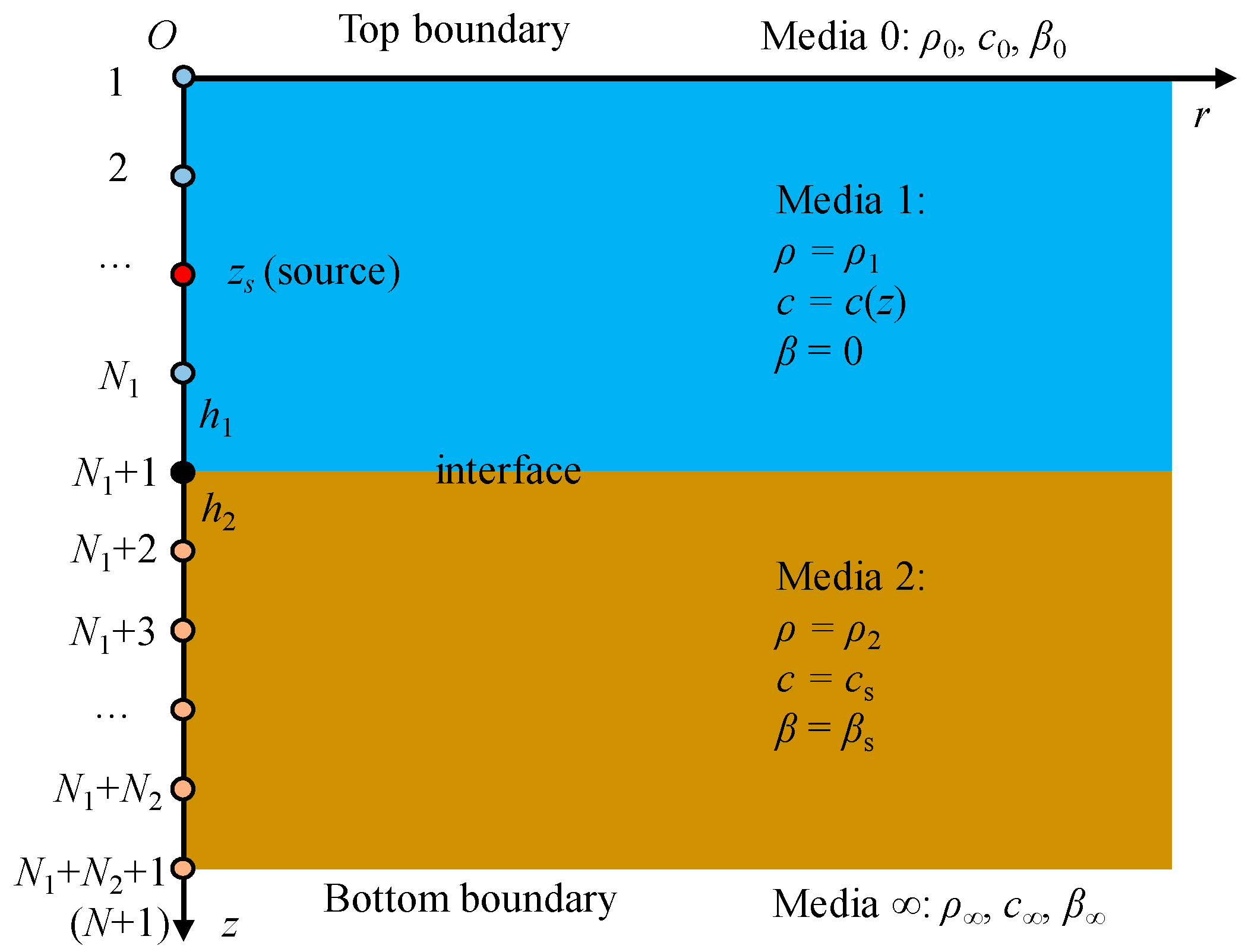
2. Mathematical Models

The pressure field excited by a time-harmonic point source in horizontally stratified oceanic environments can be modeled using Hankel integral transforms. Then, the sound pressure can be constructed by summing the contributions from individual components called normal modes, and each mode is associated with one of the solutions to the modal equation. The modal equation has an infinite number of solutions, and each solution (mode) is characterized by a mode shape function (eigenfunction) and a horizontal wavenumber (eigenvalue). Then, the acoustic pressure at any point in the cylindrical coordinate system can be calculated as the sum of the contributions of all the found modes [1]:

$$P\left(r,z\right)=\frac{\pi \mathrm{i}}{\rho \left(z_s\right)}\left[{\displaystyle \sum _{n=1}^M{\widehat{\phi }}_n\left(z_s\right){\widehat{\phi }}_n\left(z\right)H_0^{\left(1\right)}\left(k_{r,n}r\right)}\right]$$

(1)

$${\widehat{\phi }}_n\left(z\right)=\frac{{\phi }_n\left(z\right)}{\sqrt{\mathrm{i}{\phi }_n^2\left(H\right)/{\left(2\rho k_{z,n}\right)}_{\infty }+{\displaystyle {\int }_{z_0}^{z_N}{\phi }_n^2\left(z\right)/\rho dz}}}$$

(2)

where P is the complex sound pressure in the frequency-domain; r is the range coordinate from the source; z is the vertical coordinate; z_s and H are the depths of the sound source and lower boundary of the sound field, respectively; the imaginary unit number i (iota) is equal to the square root of −1; $H_0^{\left(1\right)}$ is the zero-order Hankel function of the first kind; k_r and $k_z=\sqrt{{\omega }^2/c^2-k_r^2}$ are horizontal and vertical wavenumbers, respectively, where ω = 2πf and f is the frequency of the sound source; ρ and c are the density and sound speed of the medium as functions of the depth z; the number of found modes, M, should be large enough to ensure the calculation result has sufficient precision; k_r,n and φ_n are the nth eigenvalue and its corresponding eigenfunction, respectively.

As shown in Figure 1, the densities of water and sediment are commonly treated as constants in marine environments, and thus the modal equations in the water and sediment layers can be separately formulated as

$${\phi }^{\left(2\right)}\left(z\right)+\left({\omega }^2/c_w^2-k_r^2\right)\phi \left(z\right)=0,\hspace{1em}z\in \left(0,D\right)$$

(3)

$${\phi }^{\left(2\right)}\left(z\right)+\left({\omega }^2/c_s^2-k_r^2\right)\phi \left(z\right)=0,\hspace{1em}z\in \left(D,H\right)$$

(4)

where φ⁽ⁿ⁾(z) denotes the nth derivative of φ(z) at a depth of z; D is the depth of the water column (D ≤ H); the subscripts of “w” and “s” stand for the water and sediment medium, respectively. The interface condition can be given by

$${\rho }_w^{-1}{\phi }^{\left(1\right)}\left(D^{-}\right)={\rho }_s^{-1}{\phi }^{\left(1\right)}\left(D^{+}\right)$$

(5)

where φ⁽¹⁾(D^±) denotes the limiting value of the first derivative of φ(z) at the interface as approached from z > D (D⁺) and z < D (D⁻), respectively. Furthermore, acoustic half-space (Sommerfeld radiation) conditions are introduced at the top and bottom boundaries of the sound field, respectively given by

$${\rho }_{\mathrm{w}}^{-1}{\phi }^{\left(1\right)}\left(0^{+}\right)=-\mathrm{i}{k}_{z,0}{\rho }_0^{-1}\phi \left(0\right)$$

(6)

$${\rho }_s^{-1}{\phi }^{\left(1\right)}\left(H^{-}\right)=\mathrm{i}{k}_{z,\infty }{\rho }_{\infty }^{-1}\phi \left(H\right)$$

(7)

where the subscripts “0” and “∞” indicate the homogenous half-space medium above and below the region of the sound field, respectively. If the upper half-space is assumed to be a vacuum (ρ₀ = 0), the top boundary condition can be correspondingly simplified to

$$\phi \left(0\right)=0$$

(8)

The FDM is applied to the modal equation, and its principle is to employ a Taylor series expansion to discretize the derivatives of the function φ. We can then build a system of linear algebraic equations involving the unknown solution values at grid points in the vertical direction, which can be solved numerically by direct or iterative methods. As illustrated in Figure 1, the water and sediment layers are divided into N₁ and N₂ equal intervals, respectively, and grid step sizes in the two medium layers can be calculated by h₁ = D/N₁ and h₂ = (H − D)/N₂, respectively, where N₁ and N₂ are positive integers and should be set large enough to adequately sample the modes; for instance, at least twenty points per wavelength should be set in KrakenC.

2.1. The SFD

Although the interior point scheme of the SFD is well known, the modal equation also contains the interface condition and Sommerfeld radiation boundary condition. Therefore, we will briefly deduce the SFD, including FD schemes corresponding to the interface point, the boundary point, and the interior point. In addition, this section will help one to understand the connection and differences between the NFD and the SFD more clearly.

2.1.1. Interface Scheme

The function φ at the point just above the interface ($z_{N_1+1}$ = D) can be expressed as

$$\phi \left(D-h_1\right)=\phi \left(D\right)-h_1{\phi }^{\left(1\right)}\left(D^{-}\right)+\frac{h_1^2}{2!}{\phi }^{\left(2\right)}\left(D^{-}\right)+O\left(h_1^3\right)$$

(9)

According to the modal equation of Equation (3), we have

$${\phi }^{\left(2\right)}\left(D^{-}\right)=-\left({\omega }^2/c_w^2-k_r^2\right)\phi \left(D\right)$$

(10)

Then, Equation (9) can be rewritten as

$${\phi }^{\left(1\right)}\left(D^{-}\right)=\frac{-\phi \left(D-h_1\right)}{h_1}+\frac{\phi \left(D\right)-h_1^2\left({\omega }^2/c_w^2-k_r^2\right)\phi \left(D\right)/2}{h_1}+O\left(h_1^2\right)$$

(11)

By applying a similar process as that used to derive Equation (11), we can obtain

$${\phi }^{\left(1\right)}\left(D^{+}\right)=\frac{\phi \left(D+h_2\right)}{h_2}+\frac{-\phi \left(D\right)+h_2^2\left({\omega }^2/c_s^2-k_r^2\right)\phi \left(D\right)/2}{h_2}+O\left(h_2^2\right)$$

(12)

Substituting Equations (11) and (12) into Equation (5), the interface condition can be approximated by the following FD scheme

$$\frac{\phi \left(D-h_1\right)}{{\rho }_w{h}_1}-\left(\frac{2-h_1^2{k}_{z,w}^2}{2{\rho }_w{h}_1}+\frac{2-h_2^2{k}_{z,s}^2}{2{\rho }_s{h}_2}\right)\phi \left(D\right)+\frac{\phi \left(D+h_2\right)}{{\rho }_s{h}_2}=O\left(h_1^2\right)+O\left(h_2^2\right)$$

(13)

2.1.2. Boundary Schemes

At the bottom of the acoustic field (z_N+1 = H), the backward difference formula similar to Equation (11) can be used to approximate φ⁽¹⁾(H⁻)

$${\phi }^{\left(1\right)}\left(H^{-}\right)=\frac{-\phi \left(H-h_2\right)}{h_2}+\frac{\phi \left(H\right)-h_2^2{k}_{z,s}^2\phi \left(H\right)/2}{h_2}+O\left(h_2^2\right)$$

(14)

Then, the Sommerfeld radiation condition of Equation (7) at the bottom of the sound field can be approximated as

$$\frac{\phi \left(H-h_2\right)}{{\rho }_{\mathrm{s}}{h}_2}-\left(\frac{2-h_2^2{k}_{z,s}^2}{2{\rho }_{\mathrm{s}}{h}_2}+\frac{-\mathrm{i}{k}_{z,\infty }}{{\rho }_{\infty }}\right)\phi \left(H\right)=O\left(h_2^2\right)$$

(15)

Symmetrically with the treatment of the bottom boundary condition, the forward difference formula similar to Equation (12) can be used to approximate ${\phi }^{\left(1\right)}\left(z_1^{+}\right)$ at the top of the acoustic field (z₁ = 0)

$${\phi }^{\left(1\right)}\left(z_1^{+}\right)=\frac{\phi \left(z_1+h_1\right)}{h_1}+\frac{-\phi \left(z_1\right)+h_1^2\left({\omega }^2/c_{\mathrm{w}}^2-k_r^2\right)\phi \left(z_1\right)/2}{h_1}+O\left(h_1^2\right)$$

(16)

Then, the Sommerfeld radiation condition of Equation (6) at the top of the sound field can be approximated as

$$\frac{\phi \left(z_1+h_1\right)}{{\rho }_{\mathrm{w}}{h}_1}-\left(\frac{2-h_1^2{k}_{z,\mathrm{w}}^2\left(z_1\right)}{2{\rho }_{\mathrm{w}}{h}_1}+\frac{-\mathrm{i}{k}_{z,0}}{{\rho }_0}\right)\phi \left(z_1\right)=O\left(h_1^2\right)$$

(17)

In underwater acoustics, the top boundary commonly indicates the sea surface, and then the pressure-release condition of Equation (8) can be directly used (φ(z₁) = 0).

2.1.3. Interior Point Scheme

In the water layer (0 < z < D), the coordinates of grid points in the z-direction can be expressed as z_j = (j-1)h₁ (1 < j ≤ N₁+1). By applying the Taylor expansion, the functions φ(z_j + h₁) and φ(z_j − h₁) have a power series representation about z = z_j

$$\phi \left(z_j+h_1\right)=\phi \left(z_j\right)+h_1{\phi }^{\left(1\right)}\left(z_j\right)+\frac{h_1^2}{2!}{\phi }^{\left(2\right)}\left(z_j\right)+\dots +\frac{h_1^n}{n!}{\phi }^{\left(n\right)}\left(z_j\right)+\dots$$

(18)

$$\phi \left(z_j-h_1\right)=\phi \left(z_j\right)-h_1{\phi }^{\left(1\right)}\left(z_j\right)+\frac{h_1^2}{2!}{\phi }^{\left(2\right)}\left(z_j\right)+\dots +{\left(-1\right)}^n\frac{h_1^n}{n!}{\phi }^{\left(n\right)}\left(z_j\right)+\dots$$

(19)

Adding Equations (18) and (19), we have

$$\phi \left(z_j+h_1\right)-2\phi \left(z_j\right)+\phi \left(z_j-h_1\right)-h_1^2{\phi }^{\left(2\right)}\left(z_j\right)=O\left(h_1^4\right)$$

(20)

From the modal equation in the water layer (Equation (3)), the SFD at an interior grid point z_j can be obtained

$$\phi \left(z_j+h_1\right)-\left(2-h_1^2{k}_{z,w}^2\right)\phi \left(z_j\right)+\phi \left(z_j-h_1\right)=O\left(h_1^4\right)$$

(21)

To be consistent with the interface scheme and boundary schemes, we introduce a scaling factor of 1/(ρ_wh₁) in Equation (21)

$$\frac{\phi \left(z_j+h_1\right)}{{\rho }_{\mathrm{w}}{h}_1}-\frac{2-h_1^2{k}_{z,w}^2}{{\rho }_{\mathrm{w}}{h}_1}\phi \left(z_j\right)+\frac{\phi \left(z_j-h_1\right)}{{\rho }_{\mathrm{w}}{h}_1}=O\left(h_1^3\right)$$

(22)

The SFD at an interior point in the sediment medium (D < z < H) is similar to Equation (22) (replacing ρ_w, h₁, and k_z,w with ρ_s, h₂, and k_z,s, respectively).

2.1.4. Linear System

Using Equations (13), (15), (17) and (20), a linear system corresponding to the SFD can be constructed, which is given by

$${\mathit{A}}_{\mathrm{SFD}}\mathit{\phi }=\mathbf{0}$$

(23)

where A_SFD is a complex symmetric tridiagonal matrix defined by (N = N₁ + N₂)

$${\mathit{A}}_{\mathrm{SFD}}=\left[\begin{array}{ccccccccc}{d}_1& e_2& & & & & & & \\ e_2& d_2& e_3& & & & & & \\ & \cdots & \cdots & \cdots & & & & & \\ & & e_{N_1}& d_{N_1}& e_{N_1+1}& & & & \\ & & & e_{N_1+1}& d_{N_1+1}& e_{N_1+2}& & & \\ & & & & e_{N_1+2}& d_{N_1+2}& e_{N_1+3}& & \\ & & & & & \cdots & \cdots & \cdots & \\ & & & & & & e_N& d_N& e_{N+1}\\ & & & & & & & e_{N+1}& d_{N+1}\end{array}\right]$$

(24)

and the coefficients are given by

$$d_1=-\left[1-h_1^2{k}_{z,\mathrm{w}}^2/2-\mathrm{i}{k}_{z,0}{h}_1{\rho }_{\mathrm{w}}{\rho }_0^{-1}\right]/\left({\rho }_{\mathrm{w}}{h}_1\right)$$

(25)

$$d_w=-\left(2-h_1^2{k}_{z,w}^2\right)/\left({\rho }_{\mathrm{w}}{h}_1\right),\hspace{1em}w=2,3,\dots ,N_1$$

(26)

$$d_{N_1+1}=-\left[\left(2-h_1^2{k}_{z,\mathrm{w}}^2\right)/\left(2{\rho }_w{h}_1\right)+\left(2-h_2^2{k}_{z,\mathrm{s}}^2\right)/\left(2{\rho }_s{h}_2\right)\right]$$

(27)

$$d_s=-\left(2-h_2^2{k}_{z,s}^2\right)/\left({\rho }_s{h}_2\right),\hspace{1em}s=N_1+2,N_1+3,\dots ,N$$

(28)

$$d_{N+1}=-\left[1-h_2^2{k}_{z,s}^2/2-\mathrm{i}{k}_{z,\infty }{h}_2{\rho }_s{\rho }_{\infty }^{-1}\right]/\left({\rho }_{\mathrm{s}}{h}_2\right)$$

(29)

$$e_w=1/\left({\rho }_{\mathrm{w}}{h}_1\right),\hspace{1em}w=2,\dots ,N_1+1$$

(30)

$$e_s=1/\left({\rho }_s{h}_2\right),\hspace{1em}s=N_1+2,N_1+3,\dots ,N+1$$

(31)

Because the horizontal wavenumber k_r cannot be known in advance, Equation (23) needs to be solved by shooting methods. Note that if the top boundary condition is the pressure-release condition (meaning that ρ₀ = 0 and φ(0) = 0), ${\rho }_0^{-1}$ in Equation (25) goes to infinity, and then d₁ and e₂ need to be changed to d₁ = 1 and e₂ = 0, respectively.

2.2. The NFD

From the modal equation in the water layer (Equation (3)), we have

$${\phi }^{\left(2\right)}\left(z\right)=-k_{z,w}^2\left(z\right)\phi \left(z\right)$$

(32)

$${\phi }^{\left(3\right)}\left(z\right)=-{\left(k_{z,w}^2\left(z\right)\right)}^{\left(1\right)}\phi \left(z\right)-k_{z,w}^2\left(z\right){\phi }^{\left(1\right)}\left(z\right)$$

(33)

where

$${\left(k_{z,w}^2\left(z\right)\right)}^{\left(1\right)}=\frac{d\left({\omega }^2/c_w^2\left(z\right)-k_r^2\right)}{dz}={\omega }^2\frac{d\left(c_w^{-2}\left(z\right)\right)}{dz}=-2{\omega }^2{c}_w^{-3}\left(z\right)\frac{d{c}_w\left(z\right)}{dz}$$

(34)

For shallow water acoustics, the commonly used value of the sound speed in water is a constant of 1500 m/s (such as the Pekeris waveguide problem), meaning dc_w/dz = 0. For deep water acoustics, as the sound speed typically changes weakly with depth, the absolute value of ${\left(k_{z,w}^2\left(z\right)\right)}^{\left(1\right)}$ is commonly small enough to be safely ignored. For instance, the Munk sound speed profile is widely used in deep water acoustics and has an analytical formula of

$$c_w\left(z\right)=1500\left[1+0.00737\left(\tilde{z}-1+e^{-\tilde{z}}\right)\right]$$

(35)

where $\tilde{z}=2\left(z-1300\right)/1300$. Then, the derivative of the sound speed with respect to z can be formulated as

$$\frac{d{c}_w\left(z\right)}{dz}=1500\times \frac{0.00737\times 2}{1300}\left(1-e^{-2\left(z-1300\right)/1300}\right)$$

(36)

For the low-frequency sound field, we have

$$\left|{\left(k_{z,w}^2\left(z\right)\right)}^{\left(1\right)}\right|\approx \left|\frac{-2{\omega }^2}{{1500}^3}\frac{d{c}_w\left(z\right)}{dz}\right|\le \left|2{\omega }^2\frac{0.00737\times 2}{{1500}^2\times 1300}\left(e^2-1\right)\right|=6.44e^{-11}{\omega }^2\approx 0$$

(37)

Therefore, the ${\left(k_{z,w}^2\left(z\right)\right)}^{\left(1\right)}$ term is ignored in this paper, and the second and higher derivatives of the function φ can be converted into terms of the function or its first derivative, meaning

$${\phi }^{\left(2n\right)}\left(z\right)={\left(-1\right)}^n{k}_{z,w}^{2n}\left(z\right)\phi \left(z\right)$$

(38)

$${\phi }^{\left(2n+1\right)}\left(z\right)={\left(-1\right)}^n{k}_{z,w}^{2n}\left(z\right){\phi }^{\left(1\right)}\left(z\right)$$

(39)

Furthermore, Equations (18) and (19) can be respectively rewritten as

$$\begin{array}{l}\phi \left(z_j+h_1\right)=\left[{\displaystyle \sum _{n=0}^{\infty }{\left(-1\right)}^n\frac{h_1^{2n}{k}_{z,w}^{2n}\left(z_j\right)}{\left(2n\right)!}}\right]\phi \left(z_j\right)+\left[{\displaystyle \sum _{n=0}^{\infty }{\left(-1\right)}^n\frac{h_1^{2n+1}{k}_{z,w}^{2n+1}\left(z_j\right)}{\left(2n+1\right)!}}\right]\frac{{\phi }^{\left(1\right)}\left(z_j\right)}{k_{z,\mathrm{w}}\left(z_j\right)}\\ \hspace{1em}\hspace{1em}\hspace{1em}\hspace{1em}=\cos \left(h_1{k}_{z,w}\left(z_j\right)\right)\phi \left(z_j\right)+k_{z,w}^{-1}\left(z_j\right)\mathrm{s}\mathrm{i}\mathrm{n}\left(h_1{k}_{z,w}\left(z_j\right)\right){\phi }^{\left(1\right)}\left(z_j\right)\end{array}$$

(40)

$$\phi \left(z_j-h_1\right)=\cos \left(h_1{k}_{z,w}\left(z_j\right)\right)\phi \left(z_j\right)-k_{z,w}^{-1}\left(z_j\right)\mathrm{s}\mathrm{i}\mathrm{n}\left(h_1{k}_{z,w}\left(z_j\right)\right){\phi }^{\left(1\right)}\left(z_j\right)$$

(41)

2.2.1. Interface Scheme

Using Equation (41), the function φ at the point just above the interface ($z_{N_1+1}$ = D) can be expressed as

$$\phi \left(D-h_1\right)=\cos \left(h_1{k}_{z,w}\left(D^{-}\right)\right)\phi \left(D\right)-k_{z,w}^{-1}\left(D^{-}\right)\mathrm{s}\mathrm{i}\mathrm{n}\left(h_1{k}_{z,w}\left(D^{-}\right)\right){\phi }^{\left(1\right)}\left(D^{-}\right)$$

(42)

and thus

$${\phi }^{\left(1\right)}\left(D^{-}\right)=-\frac{\phi \left(D-h_1\right)-\cos \left(h_1{k}_{z,w}\left(D^{-}\right)\right)\phi \left(D\right)}{k_{z,w}^{-1}\left(D^{-}\right)\sin \left(h_1{k}_{z,w}\left(D^{-}\right)\right)}$$

(43)

Similarly, using Equation (40), we have (c_s is commonly treated as a constant)

$$\phi \left(D+h_2\right)=\cos \left(h_2{k}_{z,s}\right)\phi \left(D\right)+k_{z,s}^{-1}\sin \left(h_2{k}_{z,s}\right){\phi }^{\left(1\right)}\left(D^{+}\right)$$

(44)

and thus

$${\phi }^{\left(1\right)}\left(D^{+}\right)=\frac{\phi \left(D+h_2\right)-\cos \left(h_2{k}_{z,s}\right)\phi \left(D\right)}{k_{z,s}^{-1}\sin \left(h_2{k}_{z,s}\right)}$$

(45)

then, Equation (5) can then be approximated by the following FD scheme

$$\frac{\phi \left(D-h_1\right)}{{\rho }_w{k}_{z,w}^{-1}\left(D^{-}\right)\sin \left(h_1{k}_{z,w}\left(D^{-}\right)\right)}-\left(\frac{\cot \left(h_1{k}_{z,w}\left(D^{-}\right)\right)}{{\rho }_w{k}_{z,w}^{-1}\left(D^{-}\right)}+\frac{\cot \left(h_2{k}_{z,s}\right)}{{\rho }_s{k}_{z,s}^{-1}}\right)\phi \left(D\right)+\frac{\phi \left(D+h_2\right)}{{\rho }_s{k}_{z,s}^{-1}\sin \left(h_2{k}_{z,s}\right)}=0$$

(46)

If ρ_w = ρ_s, c_w = c_s, and h₁ = h₂, then the interface condition scheme of Equation (46) will be equivalent to the interior scheme of Equation (53). If the unnormalized sinc function is used in Equation (46), mathematically defined as

$$\mathrm{sinc}\left(x\right)=\left\{\begin{array}{cc}1& \mathrm{for} x=0\\ \sin \left(x\right)/x& \mathrm{otherwise}\end{array}\right.$$

(47)

then Equation (46) can be transformed into

$$\frac{\phi \left(D-h_1\right)}{{\rho }_w{h}_1\mathrm{sinc}\left(h_1{k}_{z,w}\left(D^{-}\right)\right)}-\left(\frac{\cos \left(h_1{k}_{z,w}\left(D^{-}\right)\right)}{{\rho }_w{h}_1\mathrm{sinc}\left(h_1{k}_{z,w}\left(D^{-}\right)\right)}+\frac{\cos \left(h_2{k}_{z,s}\right)}{{\rho }_s{h}_2\mathrm{sinc}\left(h_2{k}_{z,s}\right)}\right)\phi \left(D\right)+\frac{\phi \left(D+h_2\right)}{{\rho }_s{h}_2\mathrm{sinc}\left(h_2{k}_{z,s}\right)}=0$$

(48)

2.2.2. Boundary Schemes

At the bottom of the acoustic field, the backward difference formula similar to Equation (43) can be used to approximate φ⁽¹⁾(H⁻)

$${\phi }^{\left(1\right)}\left(H^{-}\right)=-\frac{\phi \left(H-h_2\right)-\cos \left(h_2{k}_{z,s}\right)\phi \left(H\right)}{k_{z,s}^{-1}\sin \left(h_2{k}_{z,s}\right)}$$

(49)

Then, the Sommerfeld radiation condition of Equation (7) at the bottom of the sound field can be approximated as

$$\frac{\phi \left(H-h_2\right)}{{\rho }_{\mathrm{s}}{h}_2\mathrm{sinc}\left(h_2{k}_{z,s}\right)}-\left[\frac{\cos \left(h_2{k}_{z,s}\right)}{{\rho }_{\mathrm{s}}{h}_2\mathrm{sinc}\left(h_2{k}_{z,s}\right)}+\frac{-\mathrm{i}{k}_{z,\infty }}{{\rho }_{\infty }}\right]\phi \left(H\right)=0$$

(50)

Symmetrically with the treatment of the bottom boundary condition, the forward difference formula similar to Equation (45) can be used to approximate ${\phi }^{\left(1\right)}\left(z_1^{+}\right)$ at the top of the acoustic field (z₁ = 0)

$${\phi }^{\left(1\right)}\left(z_1^{+}\right)=\frac{\phi \left(z_1+h_1\right)-\cos \left(h_1{k}_{z,\mathrm{w}}\left(z_1\right)\right)\phi \left(z_1\right)}{h_1\mathrm{sinc}\left(h_1{k}_{z,\mathrm{w}}\left(z_1\right)\right)}$$

(51)

Then, the Sommerfeld radiation condition of Equation (6) at the top of the sound field can be approximated as

$$\frac{\phi \left(z_1+h_1\right)}{{\rho }_{\mathrm{w}}{h}_1\mathrm{sinc}\left(h_1{k}_{z,\mathrm{w}}\left(z_1\right)\right)}-\left[\frac{\cos \left(h_1{k}_{z,\mathrm{w}}\left(z_1\right)\right)}{{\rho }_{\mathrm{w}}{h}_1\mathrm{sinc}\left(h_1{k}_{z,\mathrm{w}}\left(z_1\right)\right)}+\frac{-\mathrm{i}{k}_{z,0}}{{\rho }_0}\right]\phi \left(z_1\right)=0$$

(52)

If the top boundary indicates the sea surface, the pressure-release condition can be directly used, meaning φ(z₁) = 0.

2.2.3. Interior Point Scheme

The FD scheme at an interior grid point z_j in the water layer can be obtained by adding Equations (40) and (41)

$$\phi \left(z_j+h_1\right)-2\cos \left(h_1{k}_{z,w}\left(z_j\right)\right)\phi \left(z_j\right)+\phi \left(z_j-h_1\right)=0$$

(53)

The FD scheme at an interior point in the sediment medium (D< z < H) is similar to Equation (53) (replacing h₁ and k_z,w with h₂ and k_z,s, respectively).

2.2.4. Linear System

Using Equations (48), (50), (52), and (53), a linear system according to the NFD can be built, given by

$${\mathit{A}}_{\mathrm{NFD}}\mathit{\phi }=0$$

(54)

where A_NFD is a complex asymmetric tridiagonal matrix defined by (N = N₁ + N₂)

$${\mathit{A}}_{\mathrm{SFD}}=\left[\begin{array}{ccccccccc}{d}_1& e_2& & & & & & & \\ 1& d_2& 1& & & & & & \\ & \cdots & \cdots & \cdots & & & & & \\ & & 1& d_{N_1}& 1& & & & \\ & & & e_{N_1+1}& d_{N_1+1}& e_{N_1+2}& & & \\ & & & & 1& d_{N_1+2}& 1& & \\ & & & & & \cdots & \cdots & \cdots & \\ & & & & & & 1& d_N& 1\\ & & & & & & & e_{N+1}& d_{N+1}\end{array}\right]$$

(55)

and the coefficients are given by

$$d_1=-\left[\cos \left(h_1{k}_{z,\mathrm{w}}\left(z_1\right)\right)/\left({\rho }_{\mathrm{w}}{h}_1\mathrm{sinc}\left(h_1{k}_{z,\mathrm{w}}\left(z_1\right)\right)\right)-\mathrm{i}{k}_{z,0}/{\rho }_0\right]$$

(56)

$$d_w=-2\cos \left(h_1{k}_{z,w}\left(z_i\right)\right),\hspace{1em}w=2,3,\dots ,N_1$$

(57)

$$d_{N_1+1}=-\left(\frac{\cos \left(h_1{k}_{z,w}\left(D^{-}\right)\right)}{{\rho }_w{h}_1\mathrm{sinc}\left(h_1{k}_{z,w}\left(D^{-}\right)\right)}+\frac{\cos \left(h_2{k}_{z,s}\right)}{{\rho }_s{h}_2\mathrm{sinc}\left(h_2{k}_{z,s}\right)}\right)$$

(58)

$$d_s=-2\cos \left(h_2{k}_{z,s}\right),\hspace{1em}s=N_1+2,N_1+3,\dots ,N$$

(59)

$$d_{N+1}=-\left[\cos \left(h_2{k}_{z,s}\right)/\left({\rho }_{\mathrm{s}}{h}_2\mathrm{sinc}\left(h_2{k}_{z,s}\right)\right)-\mathrm{i}{k}_{z,\infty }/{\rho }_{\infty }\right]$$

(60)

$$e_w=1/\left[{\rho }_{\mathrm{w}}{h}_1\mathrm{sinc}\left(h_1{k}_{z,\mathrm{w}}\left(z_w\right)\right)\right],\hspace{1em}w=2,N_1+1$$

(61)

$$e_s=1/\left[{\rho }_{\mathrm{s}}{h}_2\mathrm{sinc}\left(h_2{k}_{z,s}\right)\right],\hspace{1em}s=N_1+2,N+1$$

(62)

Similar to the matrix A_SFD, if the top boundary condition is the pressure-release condition, then d₁ and e₂ in the A_NFD need to be changed to d₁ = 1 and e₂ = 0, respectively. Since both A_SFD and A_NFD are tridiagonal matrices, they can be solved using the forward elimination and backward substitution algorithms. In addition, to limit the amount of computation required to form the matrix A_NFD, the trigonometric functions are calculated using truncated series expansions, meaning (L = 6 in this paper)

$$\cos \left(\theta \right)={\displaystyle \sum _{l=0}^L{\left(-1\right)}^l\frac{{\theta }^{2l}}{\left(2l\right)!}}+O\left({\theta }^{2l+2}\right)$$

(63)

$$\mathrm{sinc}\left(\theta \right)=\frac{\sin \left(\theta \right)}{\theta }={\displaystyle \sum _{l=0}^L{\left(-1\right)}^l\frac{{\theta }^{2l}}{\left(2l+1\right)!}}+O\left({\theta }^{2l+2}\right)$$

(64)

3. Test Cases

Three test cases were carried out to compare the performance of the NFD to that of the SFD, including the plane-wave reflection case independent of the KrakenC code, the Pekeris waveguide case with a constant sound speed of water, and the Munk waveguide case with a varying sound speed profile in the water layer. For testing the last two cases, the KrakenC code was modified, and one could choose either the original SFD or the NFD. It should be mentioned that the original KrakenC code has restrictions on the PPW: the recommended PPW is greater than 20 (20 by default), and the minimum is 10; in contrast, the PPW in the modified KrakenC code can be less than 10.

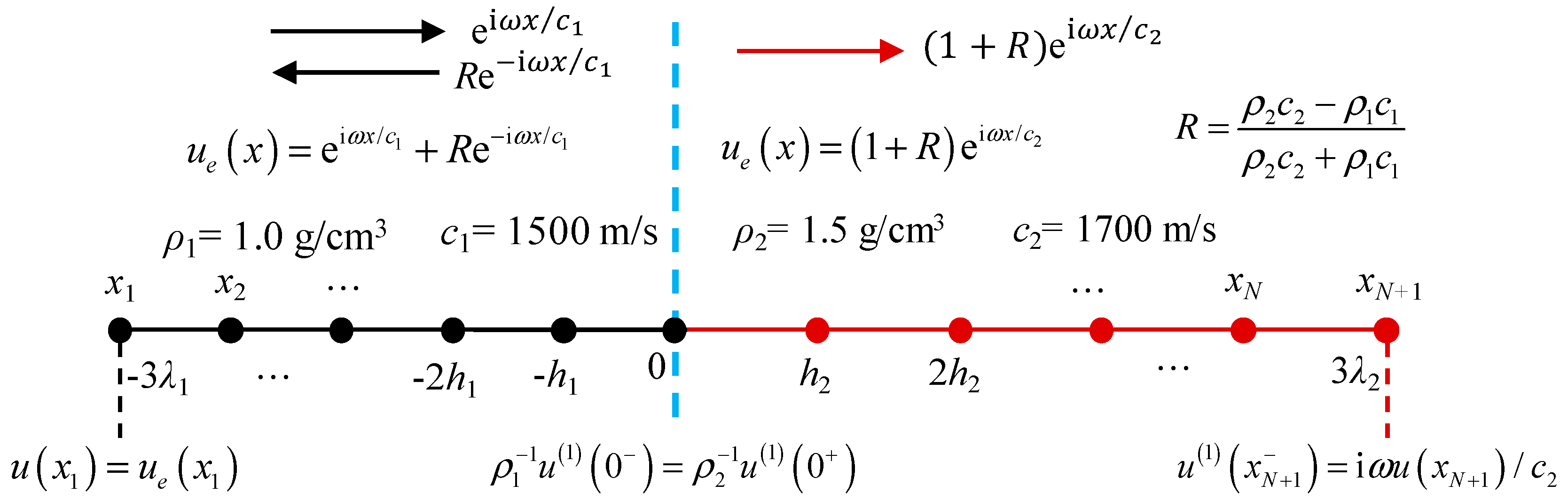
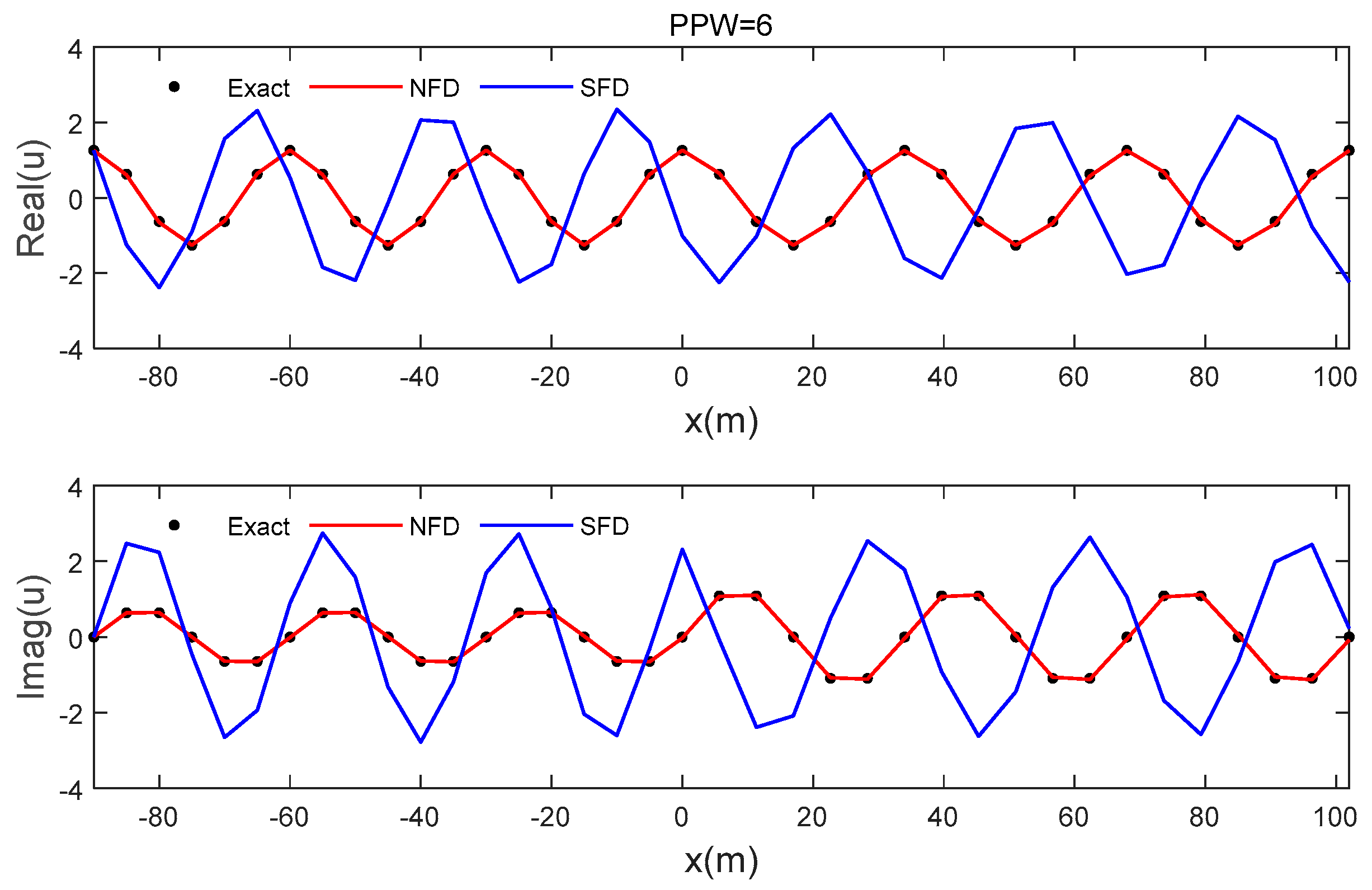
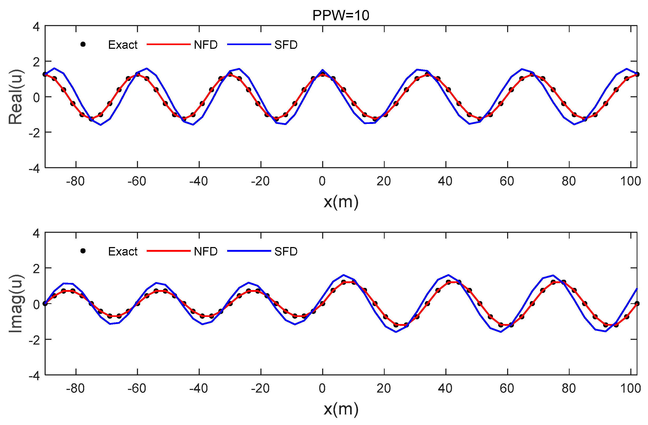
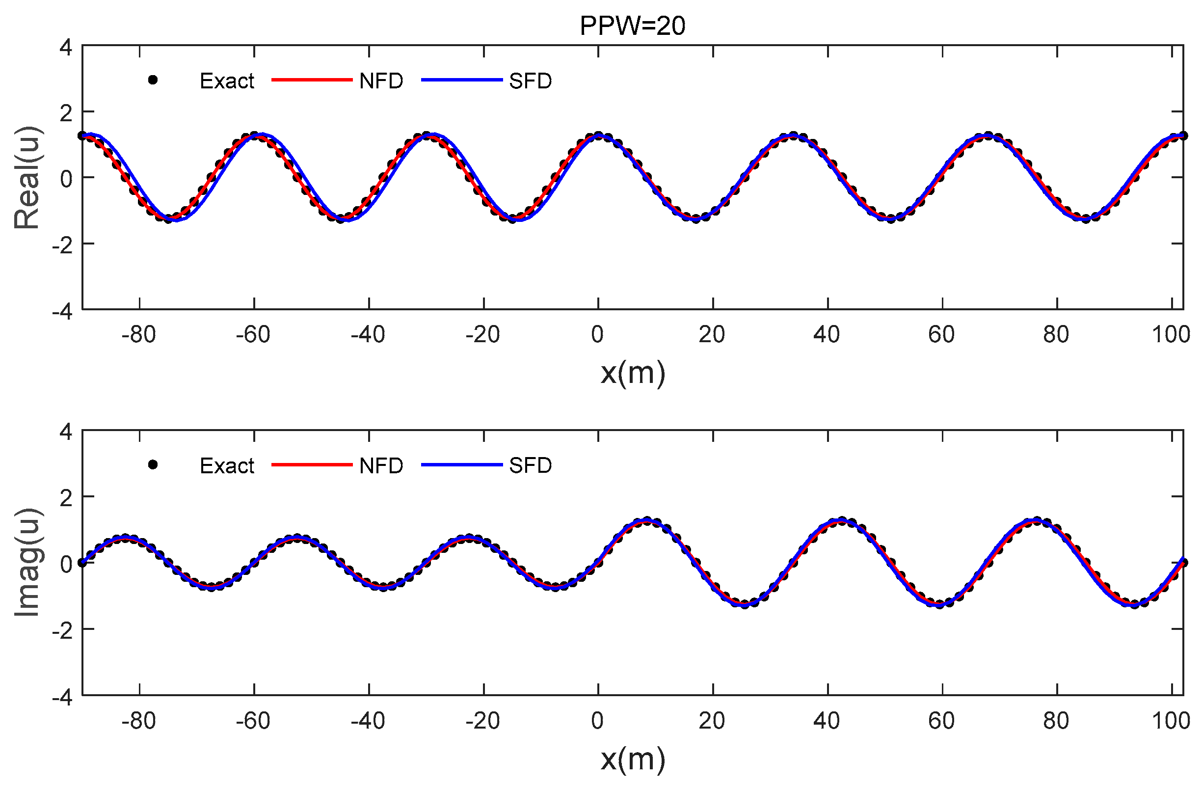
3.1. Plane-Wave Reflection

As shown in Figure 2, we consider a time-harmonic sound wave that only propagates in both the positive x and negative x directions. This acoustic propagation problem can be modeled using the following one-dimensional (1D) Helmholtz equation in the frequency-domain

$$\rho \left(x\right)\frac{\partial }{\partial x}\left(\frac{1}{\rho \left(x\right)}\frac{\partial u}{\partial x}\right)+\frac{{\omega }^2}{c^2\left(x\right)}u\left(x\right)=0,\hspace{1em}x\in \left[-3{\lambda }_1,3{\lambda }_2\right]$$

(65)

where u(x) is the sound pressure function; λ₁ and λ₂ are the wavelengths in the regions of x < 0 and x > 0, respectively; the density ρ(x) and the sound speed c(x) are piecewise constants, respectively:

$$\rho \left(x\right)=\left\{\begin{array}{c}{\rho }_1=1.0 \mathrm{g}/\mathrm{c}{\mathrm{m}}^3\\ {\rho }_2=1.5 \mathrm{g}/\mathrm{c}{\mathrm{m}}^3\end{array}\begin{array}{c},\\ ,\end{array}\begin{array}{c} x<0\\ x>0\end{array}\right.$$

(66)

$$c\left(x\right)=\left\{\begin{array}{c}{c}_1=1500 \mathrm{m}/\mathrm{s}\\ c_2=1700 \mathrm{m}/\mathrm{s}\end{array}\begin{array}{c},\\ ,\end{array}\begin{array}{c} x<0\\ x>0\end{array}\right.$$

(67)

Then, the exact solution to Equation (65) can be given by

$$u_e\left(x\right)=\left\{\begin{array}{c}{\mathrm{e}}^{\mathrm{i}\omega x/c_1}+R{\mathrm{e}}^{-\mathrm{i}\omega x/c_1}\\ \left(1+R\right){\mathrm{e}}^{\mathrm{i}\omega x/c_2}\end{array}\begin{array}{c},\\ ,\end{array}\begin{array}{c} x<0\\ x\ge 0\end{array}\right.$$

(68)

where the reflection coefficient R = (ρ₂c₂ − ρ₁c₁)/(ρ₂c₂ + ρ₁c₁) and ω = 2πf (f = 50 Hz in this case). Ensuring that the interface position (x = 0) corresponds to a grid point, the interface condition can be expressed similarly to Equation (5):

$${\rho }_1^{-1}{u}^{\left(1\right)}\left(0^{-}\right)={\rho }_2^{-1}{u}^{\left(1\right)}\left(0^{+}\right)$$

(69)

In each of the two regions of x < 0 and x > 0, Equation (65) can be discretized at evenly spaced grid points, and the grid step sizes are calculated respectively by

$$h_1={\lambda }_1/PPW=c_1/f/PPW$$

(70)

$$h_2={\lambda }_2/PPW=c_2/f/PPW$$

(71)

Then, the grid step number in each region can be given by N₁ = 3λ₁/h₁ = 3PPW and N₂ = 3λ₂/h₂ = 3PPW, respectively. The Dirichlet boundary condition is set at the left boundary (x₁ = −3λ₁), and the solution at the left boundary is given by using Equation (68), which means

$$u\left(x_1\right)=u_e\left(x_1\right)$$

(72)

The Robin (Sommerfeld radiation) boundary condition is set at the right boundary (x_N+1 = 3λ₂), and we have a similar equation to Equation (7) (herein ρ_s = ρ_∞ = ρ₂)

$$u^{\left(1\right)}\left(x_{N+1}^{-}\right)=\mathrm{i}\omega u\left(x_{N+1}\right)/c_2$$

(73)

Equations (65), (69), (72) and (73) can be discretized using the SFD or the NFD. It should be noted that the horizontal wavenumber is not included in these equations, equivalent to k_r = 0 in Equations (3), (4) and (7), and thus the tridiagonal system of linear algebraic equations resulting from the SFD or the NFD can be efficiently solved by direct methods. The real and imaginary parts of the solutions calculated by the exact formula, the SFD, and the NFD with PPW = 6, 10, and 20 were shown in Figure 3, Figure 4 and Figure 5, respectively. With all PPW numbers, the solutions from the NFD match the exact ones very well; in contrast, the curve of the SFD deviates from the other two curves, but the deviation gradually decreases as the PPW increases.

The results of this case clearly show that the SFD has a relatively large numerical error in solving the 1D Helmholtz equation (similar in form to the modal equation), and at least 20 grid points per wavelength should be set to make the error within an acceptable range, consistent with KrakenC’s recommendation of PPW ≥ 20. In contrast, the solution precision at all grid points, including the interior and boundary points, of the NFD is very high even with PPW = 6, and thus replacing the SFD with the NFD is expected to improve the precision of the KrakenC model and relax its restrictions on the PPW number.

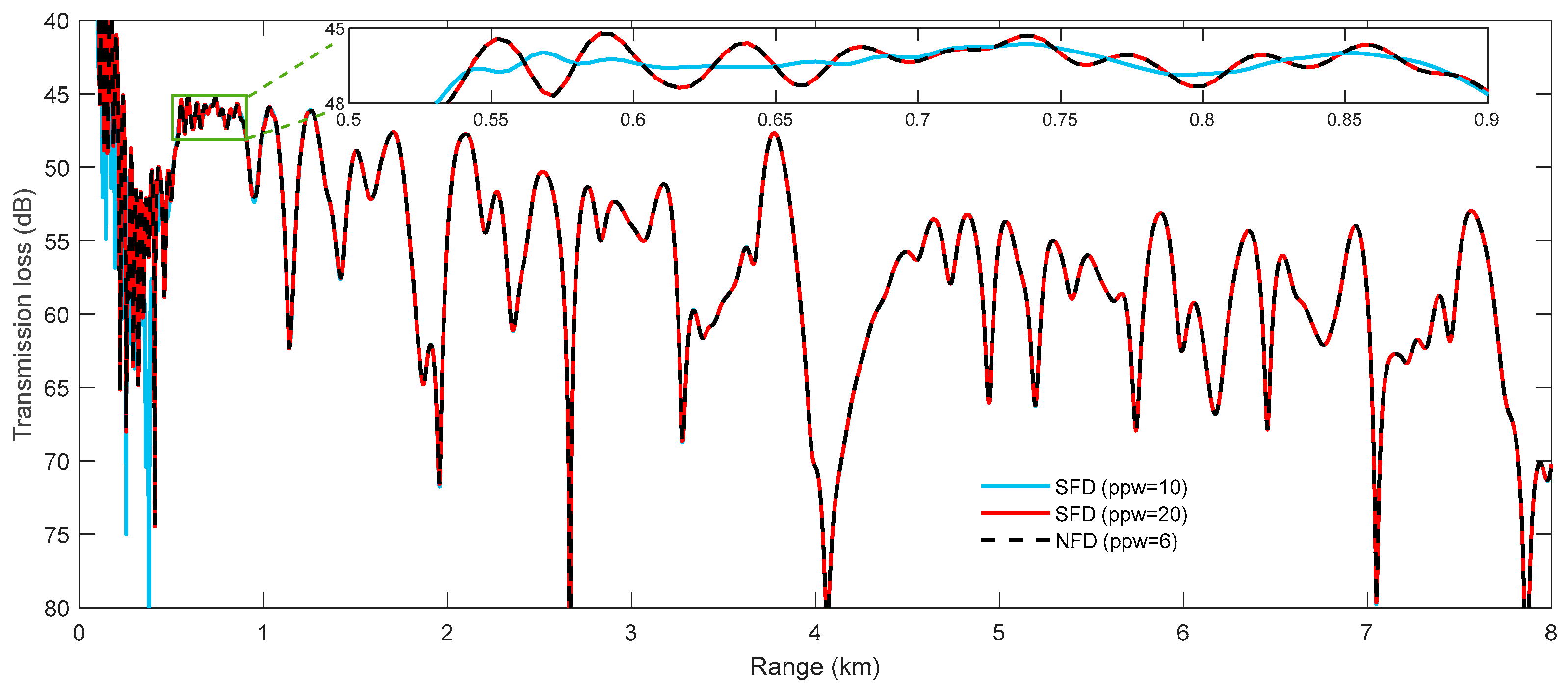
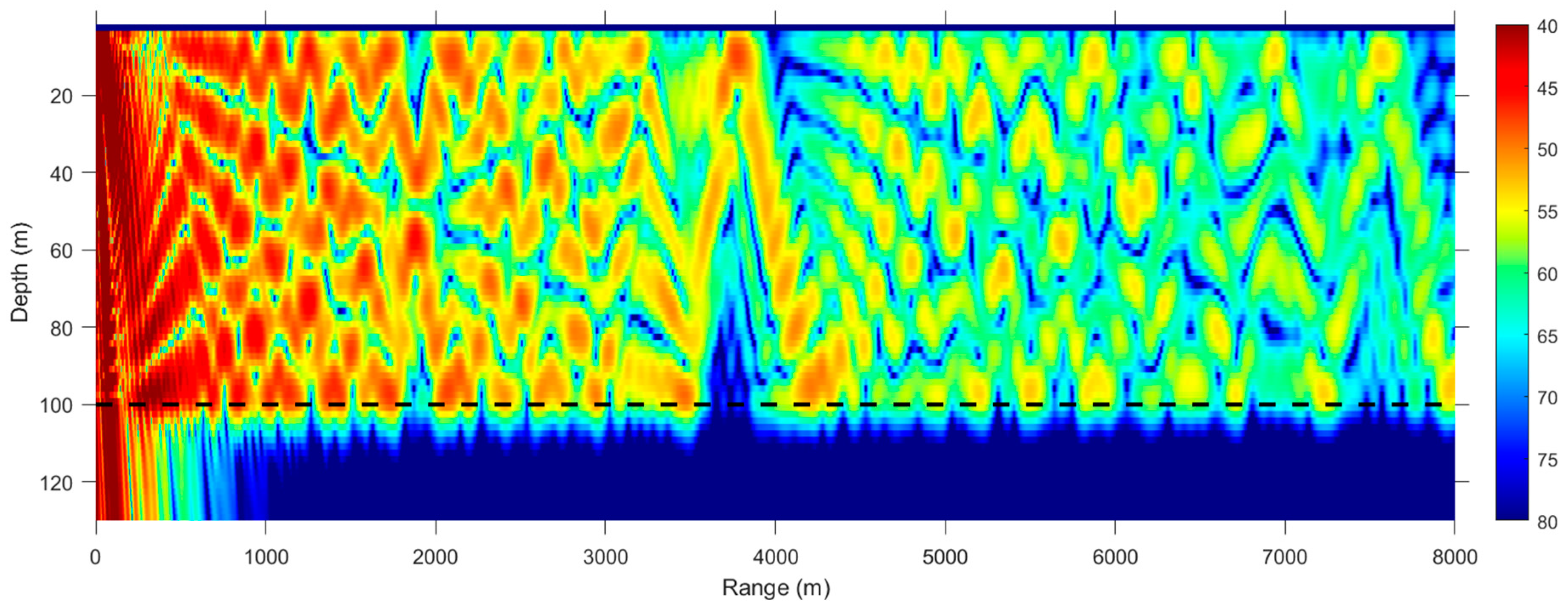
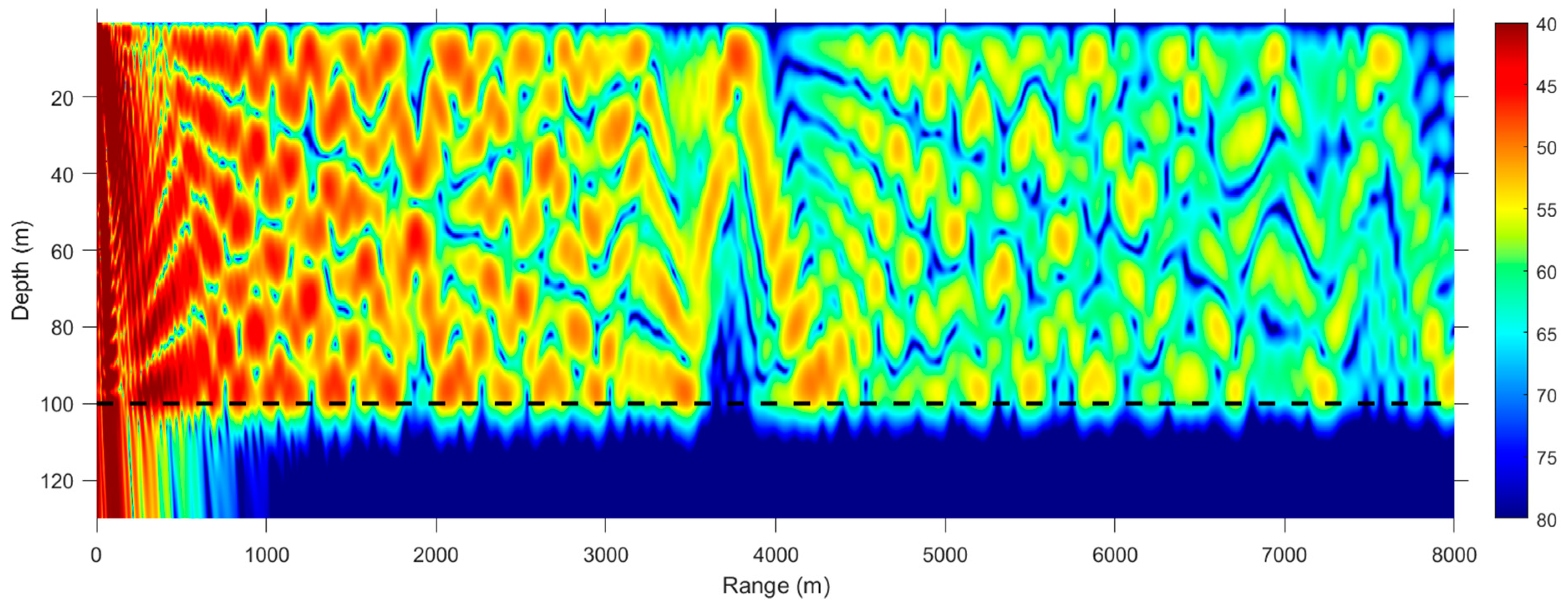
3.2. Pekeris Waveguide

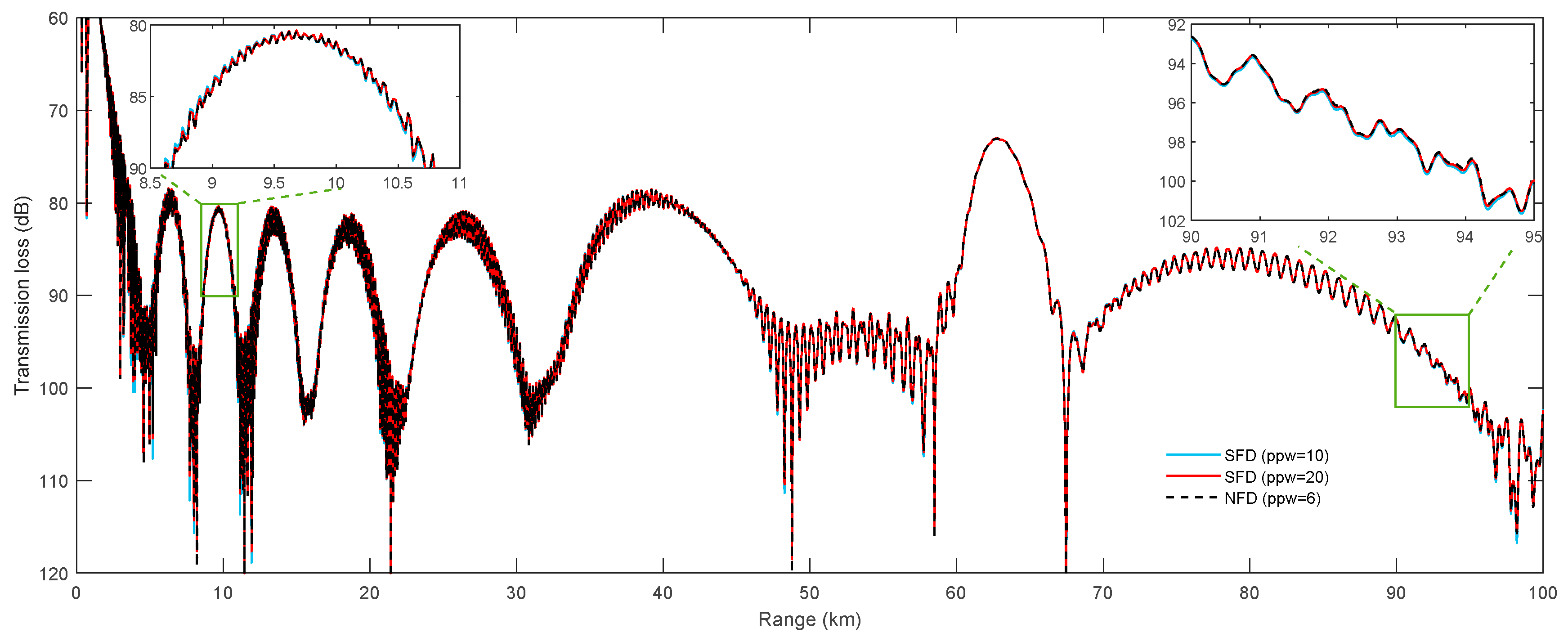
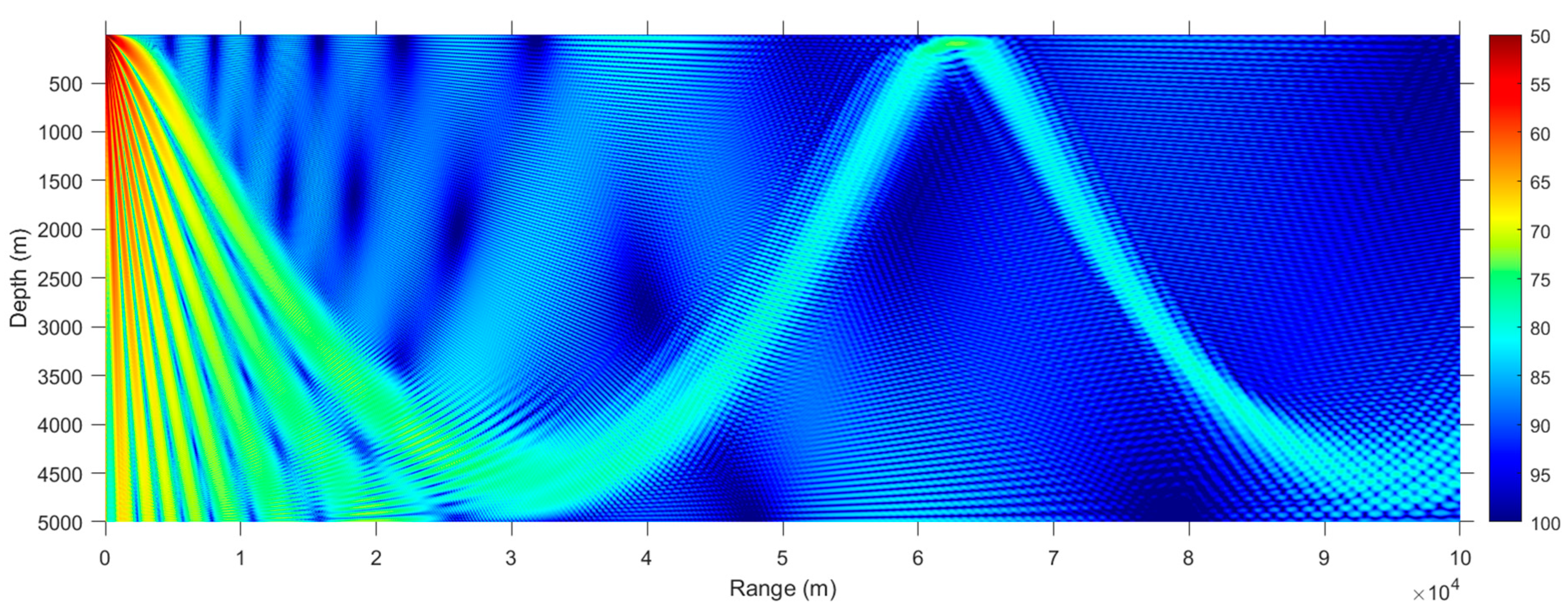
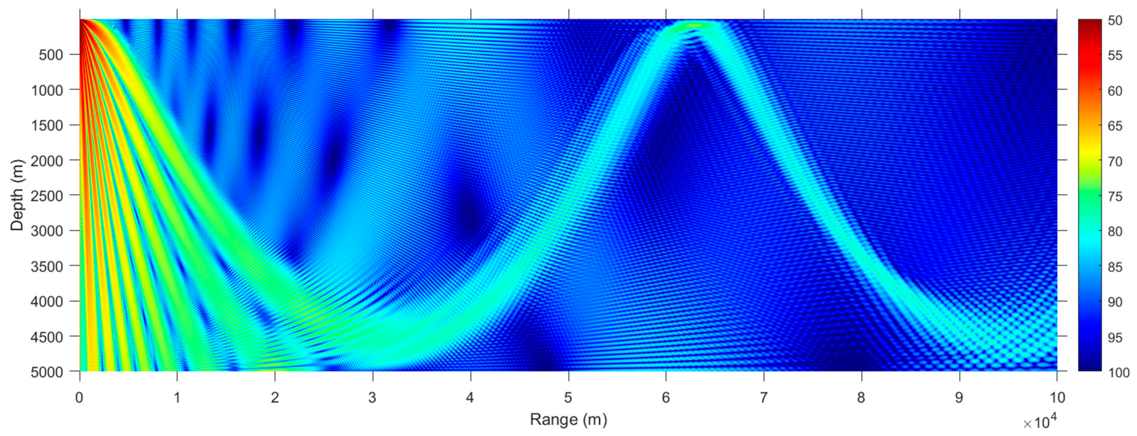
The Pekeris waveguide problem is a classical test case in underwater acoustics and consists of a homogeneous water layer over a uniform sediment half-space. Herein, the water layer is 100 m deep; the sound speed and the density of water are 1500 m/s and 1.0 g/cm³, respectively; the sediment medium has a sound speed of 1800 m/s, a density of 1.8 g/cm³, and an attenuation rate of 0.5 dB/λ. The source depth is 10 m, and the sound frequency is 150 Hz. For the root-finder in KrakenC, the lower (c_low) and upper (c_high) phase speed limits were set to 0 m/s and 10,000 m/s, respectively. It should be noted that, in this test case, the grid size of the sound field in the horizontal direction is uniform at 4 m, while the grid size in the depth direction is variable (represented by the PPW). The PPW number in the water layer is equal to that in the sediment medium.

Theoretically, the solution to the modal Equation (3) in a homogeneous water layer has the following analytical form:

$$\phi \left(z\right)=A_w^{+}{e}^{\mathrm{i}{k}_{z,w}z}+A_w^{-}{e}^{-\mathrm{i}{k}_{z,w}z},\hspace{1em}z\in \left(0,D\right)$$

(74)

At the sea surface, φ(0) = 0, and thus $A_w^{-}=-A_w^{+}\ne 0$. Therefore, at the interface point (D = 100 m), we have

$$\phi \left(D\right)=A_w^{+}\left(e^{\mathrm{i}{k}_{z,w}D}-e^{-\mathrm{i}{k}_{z,w}D}\right)=2\mathrm{i}{A}_w^{+}\sin \left(k_{z,w}D\right)$$

(75)

$${\phi }^{\left(1\right)}\left(D^{-}\right)=2\mathrm{i}{A}_w^{+}{k}_{z,w}\cos \left(k_{z,w}D\right)=k_{z,w}\cot \left(k_{z,w}D\right)\phi \left(D\right)$$

(76)

Similarly, the solution to the modal Equation (4) in the uniform sediment half-space (truncated at H = 130 m) has the following analytical form:

$$\phi \left(z\right)=A_s^{+}{e}^{\mathrm{i}{k}_{z,\mathrm{s}}z},\hspace{1em}z\in \left(D,H\right)$$

(77)

then

$${\phi }^{\left(1\right)}\left(D^{+}\right)=\mathrm{i}{k}_{z,s}{A}_s^{+}{e}^{\mathrm{i}{k}_{z,\mathrm{s}}z}=\mathrm{i}{k}_{z,s}\phi \left(D\right)$$

(78)

By substituting Equations (76) and (78) into Equation (5), one can obtain

$$\tan \left(D{k}_{z,w}\right)+\mathrm{i}{\rho }_s{k}_{z,w}/\left({\rho }_w{k}_{z,s}\right)=0$$

(79)

This equation can be used to calculate numerical errors of the approximate eigenvalues found by KrakenC in this case. For instance, if $k_{r,n}^{SFD}$ represents the nth eigenvalue found by KrakenC using the SFD, the error of this approximate eigenvalue can be calculated by applying the following formula:

$$E_n^{SFD}=\left|\tan \left(D\sqrt{{\omega }^2/c_w^2-{\left(k_{r,n}^{\mathrm{SFD}}\right)}^2}\right)+\mathrm{i}\frac{{\rho }_s\sqrt{{\omega }^2/c_w^2-{\left(k_{r,n}^{SFD}\right)}^2}}{{\rho }_w\sqrt{{\omega }^2/c_s^2-{\left(k_{r,n}^{\mathrm{SFD}}\right)}^2}}\right|$$

(80)

Utilizing the modified KrakenC code, the acoustic field of this case was simulated using the original SFD with PPW = 10, 20 and the NFD with PPW = 6, respectively, and the approximate eigenvalues found and their numerical errors are shown in

Table 1. Approximate eigenvalues and their numerical errors in the Pekeris waveguide case.

n	NFD (PPW = 6)		SFD (PPW = 10)		SFD (PPW = 20)
	${\mathit{k}}_{\mathit{r},\mathit{n}}^{\mathit{N}\mathit{F}\mathit{D}}$	${\mathit{E}}_{\mathit{n}}^{\mathit{N}\mathit{F}\mathit{D}}$	${\mathit{k}}_{\mathit{r},\mathit{n}}^{\mathit{S}\mathit{F}\mathit{D}}$	${\mathit{E}}_{\mathit{n}}^{\mathit{S}\mathit{F}\mathit{D}}$/${\mathit{E}}_{\mathit{n}}^{\mathit{N}\mathit{F}\mathit{D}}$	${\mathit{k}}_{\mathit{r},\mathit{n}}^{\mathit{S}\mathit{F}\mathit{D}}$	${\mathit{E}}_{\mathit{n}}^{\mathit{S}\mathit{F}\mathit{D}}$/${\mathit{E}}_{\mathit{n}}^{\mathit{N}\mathit{F}\mathit{D}}$
01	6.27607882022858 × 10−1–1.43856482281990 × 10−6i	4.61 × 10−5	6.27607882022858 × 10−1–1.43856482281990 × 10−6i	1.00 × 100	6.27607882022858 × 10−1–1.43856402701203 × 10−6i	1.00 × 100
02	6.25467598438263 × 10−1–5.58376723347465 × 10−6i	2.23 × 10−5	6.25467598438263 × 10−1–5.58376723347465 × 10−6i	1.00 × 100	6.25467598438263 × 10−1–5.58376768822200 × 10−6i	1.00 × 100
03	6.21873557567596 × 10−1–1.20058493848774 × 10−5i	1.87 × 10−5	6.21873557567596 × 10−1–1.20058493848774 × 10−5i	1.00 × 100	6.21873557567596 × 10−1–1.20058493848774 × 10−5i	1.00 × 100
04	6.16787314414978 × 10−1–2.02101928152842 × 10−5i	4.34 × 10−6	6.16787314414978 × 10−1–2.02101928152842 × 10−5i	1.00 × 100	6.16787314414978 × 10−1–2.02101928152842 × 10−5i	1.00 × 100
05	6.10157787799835 × 10−1–2.98445593216456 × 10−5i	7.65 × 10−6	6.10157787799835 × 10−1–2.98445593216456 × 10−5i	1.00 × 100	6.10157787799835 × 10−1–2.98445593216456 × 10−5i	1.00 × 100
06	6.01922035217285 × 10−1–4.08637897635344 × 10−5i	5.79 × 10−6	6.01922035217285 × 10−1–4.08637897635344 × 10−5i	1.00 × 100	6.01922035217285 × 10−1–4.08637897635344 × 10−5i	1.00 × 100
07	5.92005014419556 × 10−1–5.36890329385642 × 10−5i	1.96 × 10−6	5.92005014419556 × 10−1–5.36890329385642 × 10−5i	1.00 × 100	5.92005014419556 × 10−1–5.36890329385642 × 10−5i	1.00 × 100
08	5.80318808555603 × 10−1–6.95202397764660 × 10−5i	2.49 × 10−5	5.80318808555603 × 10−1–6.95202397764660 × 10−5i	1.00 × 100	5.80318808555603 × 10−1–6.95202397764660 × 10−5i	1.00 × 100
09	5.66763103008270 × 10−1–9.13004550966434 × 10−5i	6.94 × 10−6	5.66763103008270 × 10−1–9.13004550966434 × 10−5i	1.00 × 100	5.66763103008270 × 10−1–9.13004550966434 × 10−5i	1.00 × 100
10	5.51232635974884 × 10−1–1.27768376842141 × 10−4i	4.11 × 10−5	5.51232635974884 × 10−1–1.27768376842141 × 10−4i	1.00 × 100	5.51232635974884 × 10−1–1.27768376842141 × 10−4i	1.00 × 100
11	5.33674001693726 × 10−1–2.26555464905687 × 10−4i	1.35 × 10−4	5.33674001693726 × 10−1–2.26555464905687 × 10−4i	1.00 × 100	5.33674001693726 × 10−1–2.26555450353771 × 10−4i	1.00 × 100
12	4.63520050048828 × 10−1–3.02227609790862 × 10−3i	4.06 × 10−6	3.81191879510880 × 10−1–5.55971916764975 × 10−3i	5.13 × 105	4.63520050048828 × 10−1–3.02227609790862 × 10−3i	1.00 × 100
13	4.32712376117706 × 10−1–3.96012421697378 × 10−3i	5.82 × 10−6	3.36082935333252 × 10−1–7.09269661456347 × 10−3i	3.33 × 105	4.32712376117706 × 10−1–3.96012421697378 × 10−3i	1.00 × 100
14	3.97054076194763 × 10−1–5.04005001857877 × 10−3i	2.10 × 10−6	2.80377447605133 × 10−1–9.42375324666500 × 10−3i	8.70 × 105	3.97054076194763 × 10−1–5.04005001857877 × 10−3i	1.00 × 100
15	3.55095088481903 × 10−1–6.39960262924433 × 10−3i	4.50 × 10−6	2.05873236060143 × 10−1–1.39953233301640 × 10−2i	3.89 × 105	3.55095088481903 × 10−1–6.39960449188948 × 10−3i	1.01 × 100
16	3.04253190755844 × 10−1–8.32277443259955 × 10−3i	2.88 × 10−6	-	-	3.04253190755844 × 10−1–8.32277256995440 × 10−3i	1.01 × 100
17	2.38977894186974 × 10−1–1.16468686610460 × 10−2i	7.58 × 10−7	-	-	2.38977909088135 × 10−1–1.16468686610460 × 10−2i	2.28 × 100
18	1.41187623143196 × 10−1–2.14445460587740 × 10−2i	6.40 × 10−8	-	-	1.41187608242035 × 10−1–2.14445423334837 × 10−2i	2.21 × 101

. It shows that although the NFD uses a smaller PPW than the SFD, $E_n^{NFD}\le E_n^{SFD}$ for each eigenvalue. Moreover, due to the relatively large numerical errors of the SFD with PPW = 10, the 16th to 18th eigenvalues are not found by the KrakenC code using the SFD, and the errors of the 12th to 15th eigenvalues are significant.

After the approximate eigenvalues corresponding to the A_SFD or the A_NFD have been found, the eigenfunction values at all grid points for each eigenvalue can be calculated using inverse iteration methods, and then the eigenfunction values at any depth can be obtained by interpolation. Furthermore, the sound pressure field can be calculated using Equation (1). Figure 6 shows transmission loss (TL) curves at the depth of the sound source using the SFD (PPW = 10, 20) and the NFD (PPW = 6), where TL = −20 log₁₀|P| in decibels (dB) and |P| denotes the magnitude of the complex pressure P. The three curves generally match well, and the two curves obtained by using the SFD with PPW = 20 and the NFD with PPW = 6 almost coincide, indicating that the NFD with a smaller PPW number can be used to obtain the results with the same precision as the SFD with a larger PPW number, thus reducing the amount of calculation required for the NFD. In contrast, the curve obtained by using the SFD with PPW = 10 significantly deviates from the other two curves within a horizontal distance of 1 km, due to the SFD with PPW = 10 failing to accurately solve the 12th to 18th eigenvalues whose imaginary parts have large absolute values, as shown in Table 1. Because the Hankel function $H_0^{\left(1\right)}\left(k_{r,n}r\right)$ in Equation (1) vanishes quickly as the absolute value of the imaginary part of k_r,nr increases, the 12th to 18th eigenvalues only have a significant impact on the horizontal near-field, resulting in a reduction in accuracy. In contrast, the far-field results are not significantly affected.

Figure 7 and Figure 8 show TL contours in the Pekeris waveguide case using the NFD with PPW = 6 and the SFD with PPW = 20, respectively. Compared to Figure 8, Figure 7 is slightly blurred due to a relatively small number of grid points in the depth direction, but the characteristics of these two sound fields are identical.

In addition, due to the small scale of calculation in this case, the computation time of KrakenC (mainly used to calculate the eigenvalues and eigenfunctions corresponding to the modal equation) using the NFD and the SFD are both below several milliseconds, and zero seconds can even appear in multiple measurements, making it difficult to accurately measure the computation time, so a comparison analysis of calculation speed could not be provided in this case.

3.3. Munk Waveguide

The Munk waveguide problem consists of a deep water layer with a varying sound speed profile (as shown in Equation (35)) over a homogeneous sediment half-space. The depth of the water layer is 5000 m, and the water density is 1.0 g/cm³. The sediment has a sound speed of 1600 m/s, a density of 1.8 g/cm³, and an attenuation rate of 0.1 dB/λ. The depth of the sound source is 100 m, and the source frequency is 60 Hz. The lower and upper phase speed limits were set to 0 m/s and 10,000 m/s, respectively. Similarly to the Pekeris waveguide case, the grid size of the sound field in the horizontal direction is uniform at 20 m in this test case, whereas the grid size in the depth direction is variable and is represented by the PPW.

Since the error of each eigenvalue calculated by the SFD or the NFD cannot be evaluated due to the lack of a condition like Equation (80), the performance of the SFD and the NFD will only be judged from the TL results. Figure 9 shows TL curves at the depth of the sound source using the SFD (PPW = 10, 20) and the NFD (PPW = 6), respectively. The three curves generally match well, and the two curves obtained by using the SFD with PPW = 20 and the NFD with PPW = 6 almost coincide, confirming once again that the NFD with a smaller PPW number can be used to obtain the results with the same precision as the SFD with a larger PPW number. By contrast, the curve obtained by using the SFD with PPW = 10 deviates from the other two curves due to the relatively large numerical error of the SFD with a small PPW number.

Figure 10 and Figure 11 show the two TL contours in the Munk waveguide case using the NFD with PPW = 6 and the SFD with PPW = 20, respectively. Due to the large range and depth of the sound field, the grid step size in the depth direction has little effect on the sound field visualization, and the characteristics of these two sound fields are identical.

Furthermore, the computation time of KrakenC (mainly including the calculation of the eigenvalues and eigenfunctions, not including the calculation of the sound pressure field) can be significantly reduced using the NFD with smaller PPW numbers. In the Munk waveguide case, the computation time of KrakenC using the NFD with PPW = 6 and SFD with PPW = 10, 20 is 0.297 s, 0.375 s, and 0.703 s, respectively, meaning that the modified KrakenC using the NFD (PPW = 6) runs more than twice as fast as the original KrakenC using the SFD (PPW = 20) when their results have comparable accuracy.

4. Discussion

The NFD for solving the modal equation in fluid media is presented in this paper, and three test cases are carried out to verify that the NFD is generally better than the SFD. The advantages of the NFD include that it can be used with a coarser grid in the depth direction to obtain results with the same accuracy as the SFD with a finer grid, meaning that the computation time and computational effort of the KrakenC model can be reduced accordingly. Moreover, the resulting system of linear equations still has the tridiagonal structure as that derived from the SFD. It should be noted that the proposed NFD in this paper is only applicable to horizontally stratified fluid media (not including elastic boundary conditions) where the sound speed of water changes slightly with depth. Although typical underwater environments meet this condition of weak vertical variation in sound speed, some particular environments may deviate from this condition, resulting in additional numerical errors.

Future work on NFD will include applying it to other acoustic propagation models, such as wavenumber integration models [22], and expanding the types of acoustic media to which the NFD is applicable, such as elastic media and fluid media where sound speed varies moderately with depth. In addition, accurate and efficient computation of eigenvalues and eigenfunctions corresponding to the modal equation is not only related to FD schemes, but also to other relevant algorithms used to solve the eigenvalue problem. Therefore, to further improve the accuracy of normal modes, it is necessary to develop better shooting methods, Richardson extrapolation techniques, inverse iteration algorithms, and so on.

References

1. Jensen, F.B.; Kuperman, W.A.; Porter, M.B.; Schmidt, H. Computational Ocean Acoustics, 2nd ed.; Springer: New York, NY, USA, 2011. [Google Scholar] [CrossRef] [Green Version]
2. Pekeris, C.L. Theory of propagation of explosive sound in shallow water. In Geological Society of America Memoirs; Geological Society of America: Boulder, CO, USA, 1948; Volume 27, pp. 1–116. [Google Scholar] [CrossRef]
3. Porter, M.B. The KRAKEN Normal Mode Program; Naval Research Lab Washington DC: Washington, DC, USA, 1992. [Google Scholar]
4. Etter, P.C. Underwater Acoustic Modeling and Simulation; CRC Press: Boca Raton, FL, USA, 2018. [Google Scholar] [CrossRef]
5. Collis, J.M.; Frank, S.D.; Metzler, A.M.; Preston, K.S. Elastic parabolic equation and normal mode solutions for seismo-acoustic propagation in underwater environments with ice covers. J. Acoust. Soc. Am. 2016, 139, 2672–2682. [Google Scholar] [CrossRef] [PubMed]
6. DeCourcy, B.J.; Duda, T.F. A coupled mode model for omnidirectional three-dimensional underwater sound propagation. J. Acoust. Soc. Am. 2020, 148, 51–62. [Google Scholar] [CrossRef] [PubMed]
7. Westwood, E.K.; Tindle, C.T.; Chapman, N.R. A normal mode model for acousto-elastic ocean environments. J. Acoust. Soc. Am. 1996, 100, 3631–3645. [Google Scholar] [CrossRef]
8. Levinson, S.J.; Westwood, E.K.; Koch, R.A.; Mitchell, S.K.; Sheppard, C.V. An efficient and robust method for underwater acoustic normal-mode computations. J. Acoust. Soc. Am. 1995, 97, 1576–1585. [Google Scholar] [CrossRef]
9. Ding, R.; Liu, S. Underwater sound propagation for virtual environments. Vis. Comput. 2021, 37, 2797–2807. [Google Scholar] [CrossRef]
10. Jihui, W.; Zhenshan, W.; Bing, J. Numerical simulation of underwater acoustical field with directional sources based on the normal modes model. In MATEC Web Conf., Proceedings of the 2017 International Conference on Electronic Information Technology and Computer Engineering (EITCE 2017), Zhuhai, China, 23–24 September 2017; EDP Sciences: Les Ulis, France, 2017; Volume 128. [Google Scholar] [CrossRef] [Green Version]
11. Olson, A.H.; Orcutt, J.A.; Frazier, G.A. The discrete wavenumber/finite element method for synthetic seismograms. Geophys. J. Int. 1984, 77, 421–460. [Google Scholar] [CrossRef] [Green Version]
12. Tu, H.; Wang, Y.; Lan, Q.; Liu, W.; Xiao, W.; Ma, S. A Chebyshev-Tau spectral method for normal modes of underwater sound propagation with a layered marine environment. J. Sound Vib. 2021, 492, 115784. [Google Scholar] [CrossRef]
13. Tu, H.; Wang, Y.; Yang, C.; Wang, X.; Ma, S.; Xiao, W.; Liu, W. A novel algorithm to solve for an underwater line source sound field based on coupled modes and a spectral method. J. Comput. Phys. 2022, 468, 111478. [Google Scholar] [CrossRef]
14. Acoustic Toolbox. Available online: oalib.hlsresearch.com/AcousticsToolbox/ (accessed on 3 February 2023).
15. Sahu, K.S.; Jena, M.K. Combining the shooting method with an operational matrix method to solve two point boundary value problems. Int. J. Appl. Comput. Math. 2021, 7, 29. [Google Scholar] [CrossRef]
16. Dubeau, F. A remark on Richardson’s extrapolation process and numerical differentiation formulae. J. Comput. Phys. X 2019, 2, 100017. [Google Scholar] [CrossRef]
17. Porter, M.; Reiss, E.L. A numerical method for ocean-acoustic normal modes. J. Acoust. Soc. Am. 1984, 76, 244–252. [Google Scholar] [CrossRef]
18. Ipsen, I.C.F. Computing an eigenvector with inverse iteration. SIAM Rev. 1997, 39, 254–291. [Google Scholar] [CrossRef]
19. Chu, W.; Zhao, Y.; Yuan, H. A Modified inverse iteration method for computing the symmetric tridiagonal eigenvectors. Mathematics 2022, 10, 3636. [Google Scholar] [CrossRef]
20. Koessler, M.W.; Duncan, A.J.; Gavrilov, A.N. Low-frequency acoustic propagation modelling for australian range-independent environments. Acoust. Aust. 2017, 45, 331–341. [Google Scholar] [CrossRef]
21. Kun, W.; Yau Shu, W. Pollution-free finite difference schemes for non-homogeneous Helmholtz equation. Int. J. Numer. Anal. Model. 2014, 11, 787–815. [Google Scholar]
22. Liu, W.; Zhang, L.; Wang, Y.; Cheng, X.; Xiao, W. A vector wavenumber integration model of underwater acoustic propagation based on the matched interface and boundary method. J. Mar. Sci. Eng. 2021, 9, 1134. [Google Scholar] [CrossRef]
Figure 1. Sketch of the horizontally stratified marine environments.
Jmse 11 00553 g001
Figure 2. Sketch of the plane-wave reflection.
Jmse 11 00553 g002
Figure 3. The real and imaginary parts of solutions in the plane-wave reflection case with PPW = 6.
Jmse 11 00553 g003
Figure 4. The real and imaginary parts of solutions in the plane-wave reflection case with PPW = 10.
Jmse 11 00553 g004
Figure 5. The real and imaginary parts of solutions in the plane-wave reflection case with PPW = 20.
Jmse 11 00553 g005
Figure 6. TL curves at the depth of the sound source in the Pekeris waveguide case.
Jmse 11 00553 g006
Figure 7. The TL contour in the Pekeris waveguide case using the NFD with PPW = 6 (the black dotted line shows the seabed).
Jmse 11 00553 g007
Figure 8. The TL contour in the Pekeris waveguide case using the SFD with PPW = 20 (the black dotted line shows the seabed).
Jmse 11 00553 g008
Figure 9. TL curves at the depth of the sound source in the Munk waveguide case.
Jmse 11 00553 g009
Figure 10. The TL contour in the Munk waveguide case using the NFD with PPW = 6.
Jmse 11 00553 g010
Figure 11. The TL contour in the Munk waveguide case using the SFD with PPW = 20.
Jmse 11 00553 g011