Article

Large-Eddy Simulation of Wave Attenuation and Breaking on a Beach with Coastal Vegetation Modelled as Porous Medium

by
Iason A. Chalmoukis
,
Georgios A. Leftheriotis
and
Athanassios A. Dimas
*
Department of Civil Engineering, University of Patras, 26500 Patras, Greece
*
Author to whom correspondence should be addressed.
J. Mar. Sci. Eng. 2023, 11(3), 519; https://doi.org/10.3390/jmse11030519
Submission received: 18 November 2022 / Revised: 11 January 2023 / Accepted: 24 February 2023 / Published: 27 February 2023
(This article belongs to the Special Issue Estuaries, Coasts, and Seas in a Changing Climate)

Abstract

:
Erosion and flooding are the main threats for most coastal regions. Nature-based solutions, such as coastal vegetation (CV) fields, have received significant attention in recent years because they effectively dissipate wave energy while maintaining biodiversity. In this study, a porous medium model was implemented in an in-house software to simulate the three-dimensional, two-phase (water/air) flow induced by wave propagation past CV fields. First, the model was validated against experimental measurements of wave propagation past a CV field on a horizontal bed. Then, the model was used to assess the influence on wave behaviour of the equivalent porosity, neq, and the cross-shore length, LCV, of a CV field with a constant plant height on a beach with a constant bed slope. Results were obtained for the non-vegetated case (neq = 1) and five vegetated cases with different neq and LCV values. It was found that decreasing neq moves wave breaking offshore at larger depths (40% increase for the case with neq = 0.82), while it does not affect much the breaking height (4% was the largest difference). For very high neq (0.98 in the present study) and/or small LCV (83% of the wavelength just offshore of the CV field in the present study), wave breaking may occur at depths smaller than in the non-vegetated situation due to increased wave shoaling over the corresponding CV fields. The undertow distribution is strongly modified and an increased wave setup (highest for neq = 0.82) is observed for all vegetated cases in comparison to the non-vegetated one.

1. Introduction

In recent years, there has been a constantly growing interest in green infrastructure and nature-based solutions for coastal protection against erosion and flooding. Such phenomena are expected to intensify in the near future due to rising sea levels and the increasing frequency of extreme meteorological events. Natural coastal vegetation (CV) fields, e.g., seagrass and coral reefs, can attenuate the impact of coastal storms on beaches and coastal structures by dissipating the energy of waves and currents [1,2]. Furthermore, CV provides food and shelter to many organisms and contributes to the maintenance of the quality of coastal waters and the sustainable development of marine and coastal environments. Studies of wave interaction with CV fields are of fundamental importance to understanding the effect of CV on coastal protection. The majority of experimental (field and/or laboratory) and numerical studies in the literature consider the propagation of non-breaking waves past a CV field on a horizontal bed with emphasis on wave attenuation.
In experimental studies [3,4,5,6,7,8,9], the effect on wave attenuation was examined with respect to the length, LCV, of the vegetation field, the density, Nv, of the vegetation plants and the submergence ratio, hv/d, where hv is the plant height and d is the water depth. In these studies, a wide range of values of these parameters was examined. Specifically, LCV/L values were in the range 0.6–5.2, where L is the wavelength, Nv values were in the range 150–5000 plants/m2 (depending on the geometrical scale used in each study) and hv/d values were in the range 0.1–3; hv/d < 1 corresponds to cases where the vegetation canopy is submerged and hv/d > 1 to cases where the canopy is emergent. In several of these studies, the wave attenuation results were compared to the results of analytical models [10,11,12], or they were used to calibrate the parameters of analytical models. These analytical models describe wave energy dissipation due to vegetation by modelling the drag force applied to the vegetation plants. The overall conclusion is that wave attenuation increases with increasing LCV, Nv and hv/d.
In terms of numerical studies, most of them are based on the use of two-dimensional horizontal models, for example, based on the Boussinesq-type equations that do not resolve the depth-varying hydrodynamics. Karambas et al. [13] used a nonlinear Boussinesq-type model where the effect of a vegetation field was taken into account by implementing a canopy flow model and validated their model with extensive comparisons to experimental data in [3,5]. Yang et al. [14] used a nonlinear Boussinesq-type model where the effect of a vegetation field was taken into account by implementing a drag resistance term and studied wave propagation past rigid vegetation with hv/d ≥ 1. They found that, apart from the wave and plant characteristics, the wave height decay is also sensitive to the distribution pattern of plants in the CV field. In 3D (three-dimensional) numerical studies, the effect of a vegetation field is implemented using a variety of models. Mattis et al. [15] used an LES-type (large-eddy simulation) flow model where the effect of a vegetation field was taken into account by modelling the stem of each plant as a flexible beam, allowed to deform, and the flow–stem interaction was modelled using an Immersed Boundary (IB) approach. The calculated wave–energy spectra within the vegetation field were in good agreement with the experimental data. Using the same LES-type flow model, Wong et al. [16] took into account the effect of a vegetation field by implementing an appropriate sink term related to the drag resistance of the vegetation in the momentum equations. Based on a multiple-scales analysis, Wong et al. [16] also derived an analytical model of wave attenuation over a vegetation field in accordance with the model in [12]. Their analytical model and numerical results were validated against the experimental data of wave attenuation over a vegetation field on a horizontal bed. Hadadpour et al. [17] used a Reynolds-averaged Navier–Stokes (RANS)-type flow model where the effect of a vegetation field was taken into account by implementing a porous medium approach. Their numerical results were validated against experimental data of wave attenuation past a vegetation field on a horizontal bed.
The main objective of this present work was to study the effect on wave propagation of a CV field on a beach with a constant slope. Over a horizontal bed, wave attenuation is the sole hydrodynamic process, whereas over a sloped bed, wave attenuation is in competition with wave shoaling affecting wave breaking, i.e., the size of the surf zone, as well as wave setup, wave runup and wave-generated currents. To the authors’ knowledge, this is one of the very few attempts to perform 3D LES of wave propagation, attenuation and breaking over a CV field on a sloped beach bed. An in-house 3D LES-type flow model was used where the effect of a vegetation field was taken into account by implementing a porous medium approach. The numerical model is based on a High-Performance Computing (HPC) parallel architecture to reduce the computational cost. Results of the effect of the vegetation porosity and the cross-shore length of the CV field on the wave- and depth-varying flow behaviour are presented.

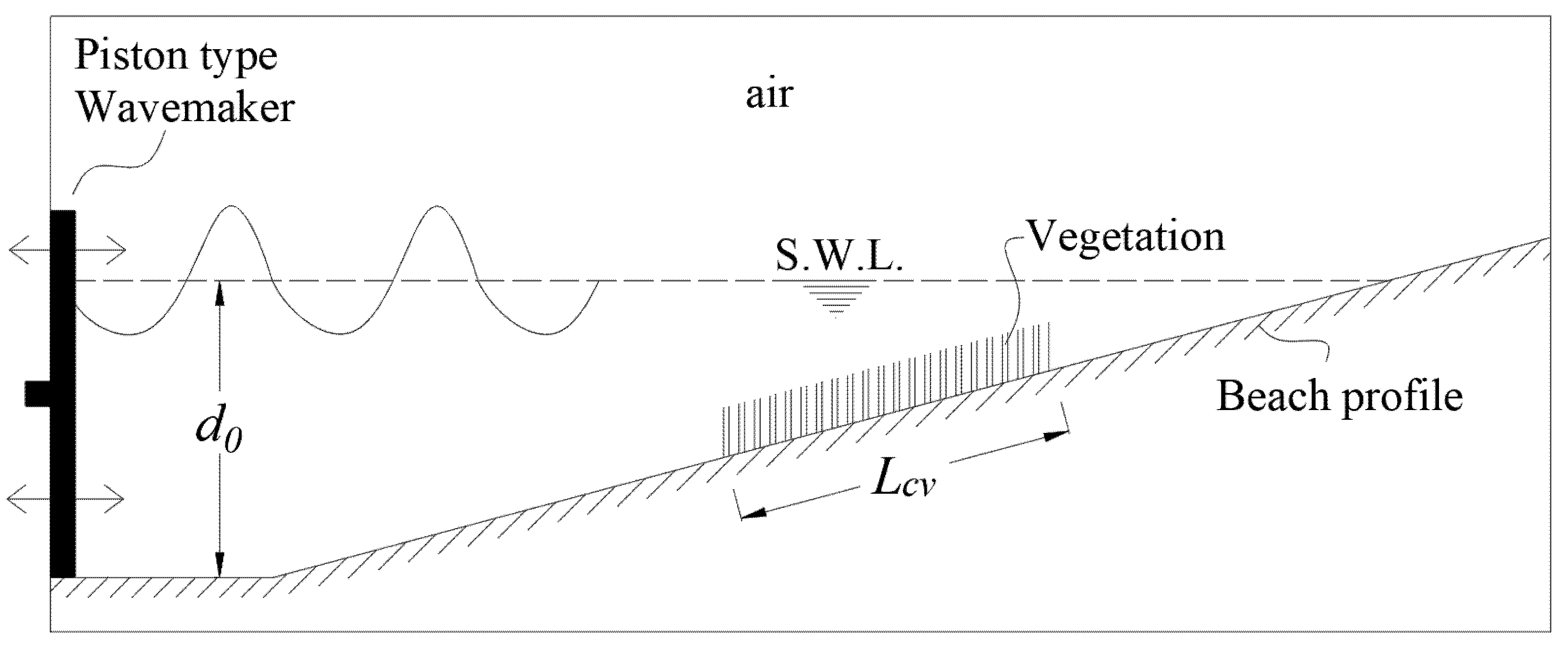
2. Materials and Methods

In the present work, the combined water and air flow are modelled as one-fluid flow governed by the 3D incompressible Navier–Stokes equations, whose formulation is based on an LES approach, and it is appropriate to model flow in porous media with constant porosity [18,19]:
u i x i = 0
1 + c A n u i t + 1 n 2 x j u i u j = 1 ρ p x i + δ i 3 Fr 2 1 n τ i j x j + 1 n 1 Re 1 ρ x j μ u i x j + u j x i a p 1 n 2 n 3 v D 2 1 Re u i β p 1 + 7.5 KC 1 n n 3 1 D u i u i u i + f i
In the above equations, xi are the Cartesian coordinates (x, y, z), t is the time, ui are the resolved velocity components in the three directions (u, v, w), cA = 0.34 (1 − n)/n is the added mass coefficient, n is the porosity, p is the total pressure, i.e., the sum of the dynamic and the hydrostatic pressure, ρ is the normalised (by the water density) fluid density, δij is the Kronecker’s delta function, Fr is the Froude number, τij are the sub-grid scale stresses associated with the LES approach, μ and ν are the normalised (by their water values) fluid dynamic viscosity and kinematic viscosity, respectively, D is the characteristic dimension of solids in the porous medium and ap and βp are empirical coefficients. The Keulegan–Carpenter number is defined as:
KC = T u i u i n D  
where T is the incident wave period. The external forcing term, fi, in Equation (2) is associated with the implementation of the IB method for the imposition of flow boundary conditions on the seabed. The 3D implementation of the IB method in Dimas and Chalmoukis [20] is used here to enforce the no-slip boundary condition on the bed surface; the bed was considered to be hydraulically smooth in the present application. An advantage of using the IB method is that a 2nd order central finite differences scheme is used on a Cartesian grid for the spatial discretization of all equations. The Navier–Stokes equations are rendered dimensionless using the characteristic water depth, d0, at the wavemaker and the gravitational acceleration, g; hence, the corresponding velocities were non-dimensionalised by (gd0)1/2 and Fr = 1.
In the present work, the LES approach is used to model the subgrid flow scales because it is more accurate than other approaches (e.g., RANS) in resolving large-scale complex flow structures in unsteady turbulent flows [21,22]. Specifically, the subgrid-scale stresses were modelled using the standard eddy-viscosity Smagorinsky model [23]:
τ i j 1 3 δ i j τ k k = 2 ν t S i j = 2 C s 2 Δ x 1 Δ x 2 Δ x 3 2 / 3 2 S i j S i j 1 / 2 S i j
where Sij = (1/2) (∂ui/∂xj + ∂uj/∂xi) is the strain-rate tensor, and Cs is the model parameter, which was set to 0.1 according to Lesieur and Metais [21]. Close to the bed, the eddy viscosity νt is reduced according to the near-wall reduction function in Van Driest [24]. The computational cost is higher in LES [22]; therefore, an HPC parallel architecture is used in the present application.
The porous medium approach is used to model the flow resistance in the CV field. To this purpose, an equivalent porosity, neq, is utilised in Equation (2) instead of n, which depends on the combined effect of CV plant density and cross-sectional dimensions. The equivalent porosity is estimated by setting 1 − neq equal to the volume of the plants divided by the total volume occupied by the CV field. Furthermore, in Equation (2), D is equal to the characteristic cross-sectional dimension of the vegetation stems. The specific approach has been reported to perform well in terms of simulating wave attenuation over a rigid vegetation field [17]. Utilising this method has many advantages. First, it is based on parameters of the vegetation field (plant density, height and cross-sectional dimensions), which can be easily measured and imported into the numerical model. Moreover, the approach is easily implemented in combination with the IB method on a Cartesian grid, which speeds up the computational time significantly, especially when implemented in parallel algorithms such as the present one. Regarding the porosity model in Equation (2), the values of the coefficients were chosen to be ap = 1000 and βp = 1.1 according to [18,25,26]. The location of the water–air interface is tracked using the level-set method that introduces a scalar variable φ, which is the perpendicular signed distance from the location of the interface. The free-surface evolution is computed by an advection equation:
φ t + u i φ = 0
where φ = 0 at the free surface. The normalised density and viscosity are defined, respectively, as:
ρ = ρ a + ρ w ρ a H φ ρ w         μ = μ a + μ w μ a H φ μ w
where subscripts w and a denote water and air, respectively, and
H ( ϕ ) = 1 , φ 0 0 , φ < 0
is a Heaviside function, which introduces sharp jump conditions for the fluid properties at the water–air interface. Thus, the corresponding conditions for the stresses across the water–air interface are internal elements of the one-fluid formulation [27].
Regarding temporal discretization, a time-splitting projection method is applied where all terms of Equation (2), except for the pressure term, are treated explicitly in the first stage, using a 2nd order Adams–Bashforth scheme for the computation of an intermediate velocity field:
u i m + 1 / 2 u i m Δ t = 3 2 H ( u i m ) 1 2 H ( u i m 1 ) + f i m + 1 / 2
In the second stage, the velocity field uim+1 is obtained by the pressure gradient as follows:
u i m + 1 = u i m + 1 / 2 Δ t ρ p m + 1
where the pressure is computed by the corresponding Poisson equation:
1 ρ p m + 1 = 1 Δ t u i m + 1 / 2
A sketch of a cross-shore vertical (2DV) plane of the computational domain with a CV field on a beach is shown in Figure 1. The domain includes both water and air layers defined at rest with respect to the still water level (S.W.L.). To simulate wave propagation, incident second-order regular waves of specific height and period are generated by a numerical piston-type wavemaker at the left boundary of the computational domain at water depth d0. For a distance equal to one wavelength downstream of the wavemaker, a relaxation zone is implemented to prevent distortions of the wave generation due to reflections from the beach [28]. Detailed information about the wave model can be found in [29].
Regarding pressure boundary conditions, a zero Neumann condition is imposed on the bottom and both streamwise boundaries of the computational domain. A Dirichlet-type condition p = ρgη is implemented at the top computational boundary, where η is the water surface elevation. Accordingly, the velocity boundary conditions are zero Neumann on the bottom and right boundaries. At the wave generation boundary (left), a Dirichlet-type condition is implemented for the streamwise velocity to be consistent with the harmonic wave generation. In the spanwise direction, periodic boundary conditions are implemented for pressure and velocities.
To ensure numerical stability, the computational time-step, Δt, is selected to satisfy both the convective (CFL) and the diffusive (VSL) criteria: CFL < 0.1 and VSL < 0.001, where
CFL i = u i Δ t Δ x i   and   VSL = Δ t Re Δ x i 2
Concerning the parallel implementation, the numerical code utilises a hybrid MPI + OpenMP approach, which can efficiently take advantage of modern supercomputing capabilities. The code has a nearly linear scaling when using up to 1200 CPU cores, achieving a parallel efficiency of 79%. For further details on the parallel implementation, the parallel efficiency and scalability of the HPC model, the interested reader is referred to Leftheriotis et al. [29].

3. Results

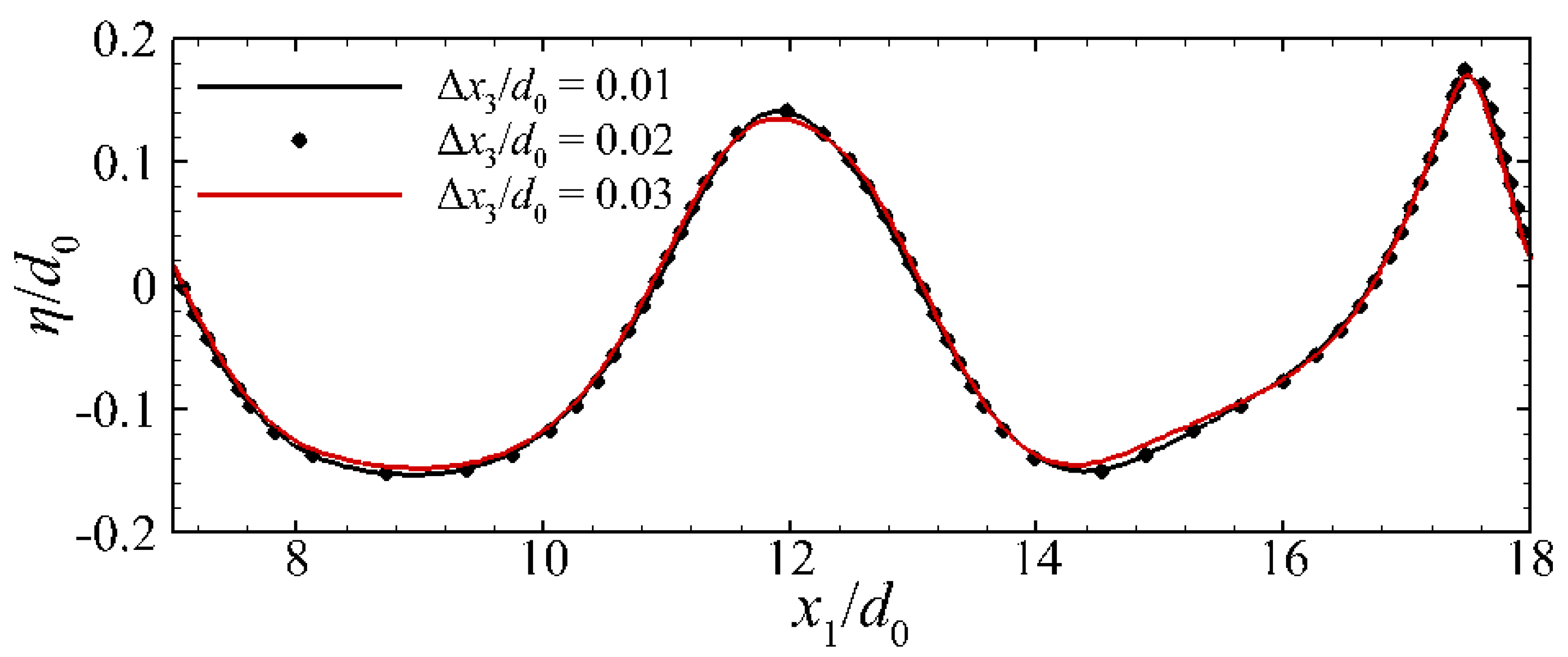
3.1. Validation of the Numerical Model

The present in-house numerical model has been previously validated in terms of hydrodynamics in Oyarzun et al. [30] and in terms of simulating complex 3D wave transformations due to the simultaneous effects of wave refraction and diffraction in Leftheriotis et al. [29]. The porous medium approach has been validated in [25] against experimental measurements for wave propagation past a submerged porous breakwater. In the present article, the porous medium model is further validated against data of wave attenuation due to the presence of a vegetation field. Augustin et al. [31] investigated experimentally and numerically the wave attenuation caused by emergent and submerged vegetation fields. Emphasis was given on the influence of different wave and vegetation parameters on the wave height decay. For the experimental configuration, they used synthetic vegetation fields consisting of rigid and flexible stem elements, both with diameters equal to 12 mm. Experimental measurements were conducted in both a narrow laboratory wave flume and a shallow-water wave basin.
The present model replicates a case in Augustin et al. [31] where the space-resolved distribution of the free-surface elevation was provided for monochromatic waves propagated past a submerged vegetation field in a narrow wave flume with dimensions of 30.5 m length, 0.9 m width and 1.2 m depth. The incident wave height was H = 12 cm, and the wave period was T = 1.5 s. The experimental validation field consisted of cylindrical stems with hv = 0.3 m and D = 12 mm. The stem density of the vegetation field was equal to 97 stems/m2. The specific configuration corresponds to neq = 0.99, which was used in this present numerical simulation. The corresponding computational domain is shown in Figure 2. The water depth at the wavemaker is d0 = 0.5 m. A flatbed region of a length equal to about two wavelengths exists downstream of the wavemaker. Half of the flatbed region corresponds to the relaxation zone, and the other half is available for fully developed wave conditions to be established before reaching the elevated bed of the vegetation field. The vegetation field is placed at a distance 17.1 m onshore of the wavemaker, and its length is equal to 6 m. A constant slope beach (1:12) is placed at the right end of the flume to dissipate the remaining wave energy and minimise wave reflection.
The relative grid spacing was selected to be uniform in all directions with values: Δx1/d0 = 0.05, Δx2/d0 = 0.025 and Δx3/d0 = 0.02. The specific discretization resulted in a grid with 1300 cells in the streamwise direction, 72 cells in the spanwise direction and 100 cells in the vertical direction. Note that the computational domain height includes both the water and air layers, with the water layer occupying about half of the total height, meaning about 50 cells in each layer.
An instant snapshot of the free-surface elevation is shown in Figure 3 (black line) after 10 wave periods. The numerical result is in good agreement with the corresponding result (red dots) in Augustin et al. [31]. The model adequately represents the wave attenuation induced by the presence of the vegetation field, as the root mean square error of the free-surface elevation is about 2.7%, while the maximum difference of the computed and experimental wave height is approximately 14% at x1/d0 ≈ 50 (Figure 3). Additionally, note that from x1/d0 = 0 to 8, the free surface is almost horizontal since the wavemaker relaxation zone is implemented in this region.

3.2. Coastal Vegetation and Wave Parameters under Study

Numerical simulations of wave propagation and breaking over a beach of constant slope tanβ = 1/15 have been performed with and without the presence of a CV field. The CV field (Figure 1) starts at a depth of 0.45 m, its height is equal to 0.1 m, and its cross-shore length, LCV, is 5.2 m in all cases but one (Case 6), where a shorter field was applied (LCV = 2.6 m) to examine the effect of LCV. The cross-shore length of the CV field was selected to be in the order of one wavelength, L, at its offshore depth as in [5]. The two different values of LCV = 8.67d0 and 4.33d0 correspond to values of about 1.66L and 0.83L, respectively. The CV parameters were selected to mimic observations of real meadows where CV density, as well as the shape and dimensions of CV stems, vary greatly. Typical CV density ranges from 62 to 556 stems/m2 [32] or as high as 4200 stems/m2 [33], whereas Posidonia Oceanica density, for example, varies from sparse, 150 stems/m2, to very dense, 700 stems/m2 [4]. In nature, the shape of the stems is like a thin blade with typical dimensions of 1 cm wide, 1 mm thick and up to 1 m long [5]. In many experimental setups, the stems are constructed as long cylindrical elements with a diameter of 3 mm [34] to 12 mm [31]. In the present laboratory scale, a characteristic diameter D = 1 mm is considered. To analyse a variety of different cases, four neq values were studied (0.82, 0.86, 0.90 and 0.98), which are representative of the range of values in [3,4,5,6,7,8,9]. In total, six cases were simulated, whose parameters are presented in Table 1.
For all cases, the Reynolds number based on the water depth at the position of the wavemaker (d0 = 0.60 m) is equal to Red = 1.3 × 10⁶. The characteristics of the incident waves correspond to laboratory scale dimensional values of H = 0.18 m and T = 1.68 s. The deep-water wave steepness is ε = 0.045, and the corresponding Iribarren number is ξo = 0.32 (spilling wave breaking).
All numerical simulations started with the fluid at rest, the first 10 wave periods of the simulations were required for the propagating waves to reach fully developed conditions, and another 10 wave periods were used for sampling and averaging. The average CPU time for each wave period was about 10 h. The simulations were executed on a petascale supercomputer at the ARIS HPC Infrastructure of the Greek Research and Technology Network (GRNET) using 600 cores.
Grid independency tests were performed for the selection of the appropriate spatial discretization of the grid. The focus was on the vertical grid spacing (Δx3/d0), which affects the most numerical results. Three different cases of grid discretization were applied and analysed, i.e., Δx3/d0 = 0.03, 0.02 and 0.01. Free-surface elevation results are presented in Figure 4 after five wave cycles from the beginning of the simulation. The numerical results for the 2 finer discretization cases (Δx3/d0 = 0.01 and 0.02) were almost identical, with maximum differences of 1.4%. The maximum differences between the 2 coarser discretization cases (Δx3/d0 = 0.02 and 0.03) were up to 5%. Thus, the second discretization (Δx3/d0 = 0.02) was selected in terms of both accuracy and efficiency.
The length of the computational domain in dimensional units was equal to 18 m, its width was 1 m, and its height was 1.2 m. After the grid independency tests, the relative grid spacing in all directions was selected to be uniform with values: Δx1/d0 = 0.05, Δx2/d0 = 0.025 and Δx3/d0 = 0.02 (Figure 4). The specific discretization resulted in a grid with 600 cells in the streamwise direction, 68 cells in the spanwise direction, 100 cells in the vertical direction and 50 cells in each layer (water or air).

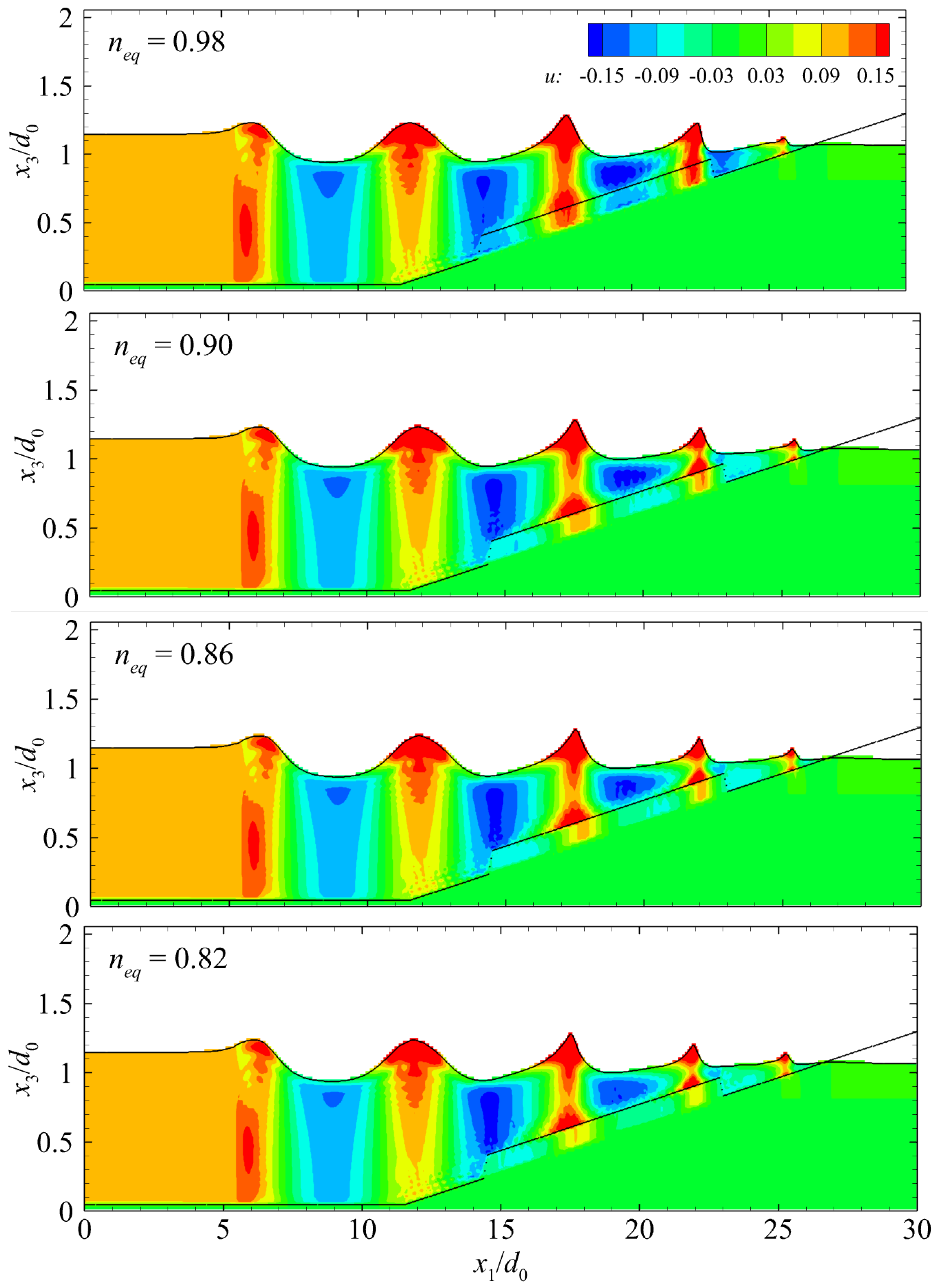
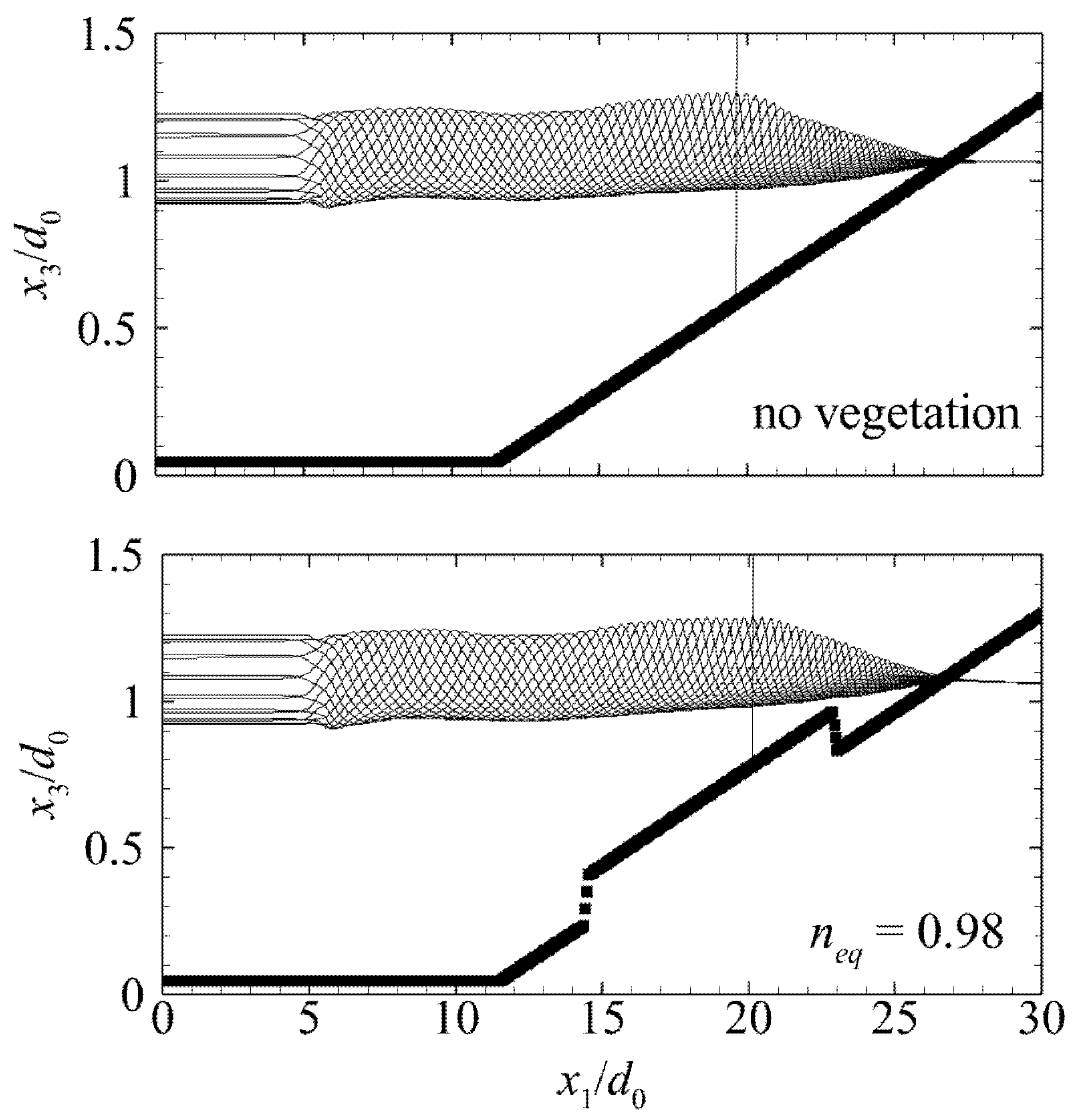
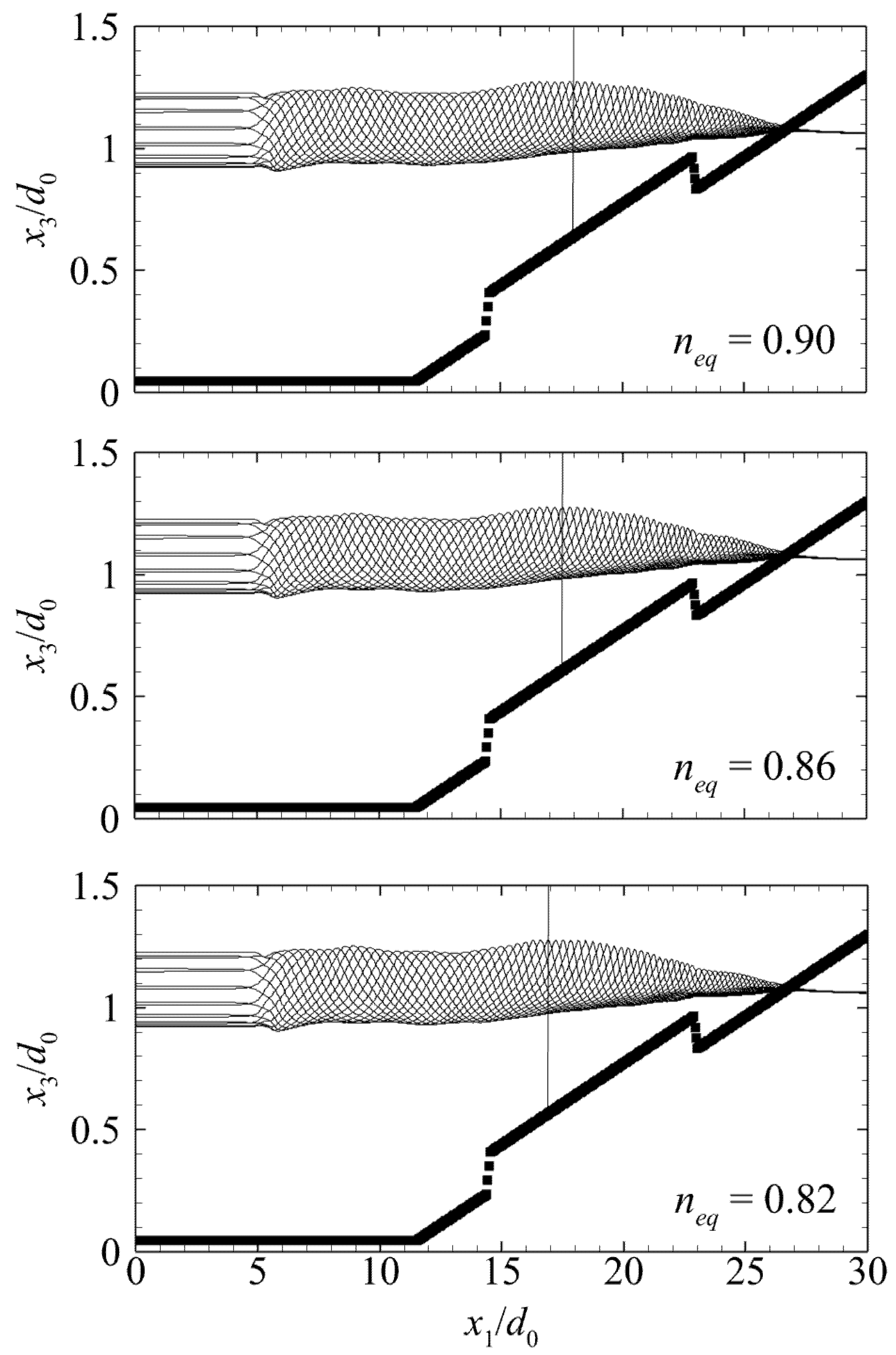
3.3. Instantaneous Velocity Field

An instantaneous 3D snapshot of waves propagating over the vegetation field (Case 5) is presented in Figure 5 after the simulation of 10 wave periods. Case 5 is the one where the CV induces the strongest wave attenuation. The streamwise velocity contours on the free surface clearly illustrate the velocity increase on the wave crest due to shoaling before wave breaking.
The streamwise velocity field on the cross-shore vertical plane, at the middle of the spanwise domain width, is presented in Figure 6 for Cases 2–5, which have the same LCV but different porosities. The porous medium model appropriately reduces velocity magnitudes inside the vegetation zone. It is interesting to note that the velocity reduction in Case 2 (neq = 0.98) is almost negligible since the porosity value is very close to unity, while as the CV field becomes denser (Cases 3–5), the velocity reduction increases. This highlights the importance of the correct estimation/calibration of the vegetation parameters in order to correctly model the CV effect on waves and flow.

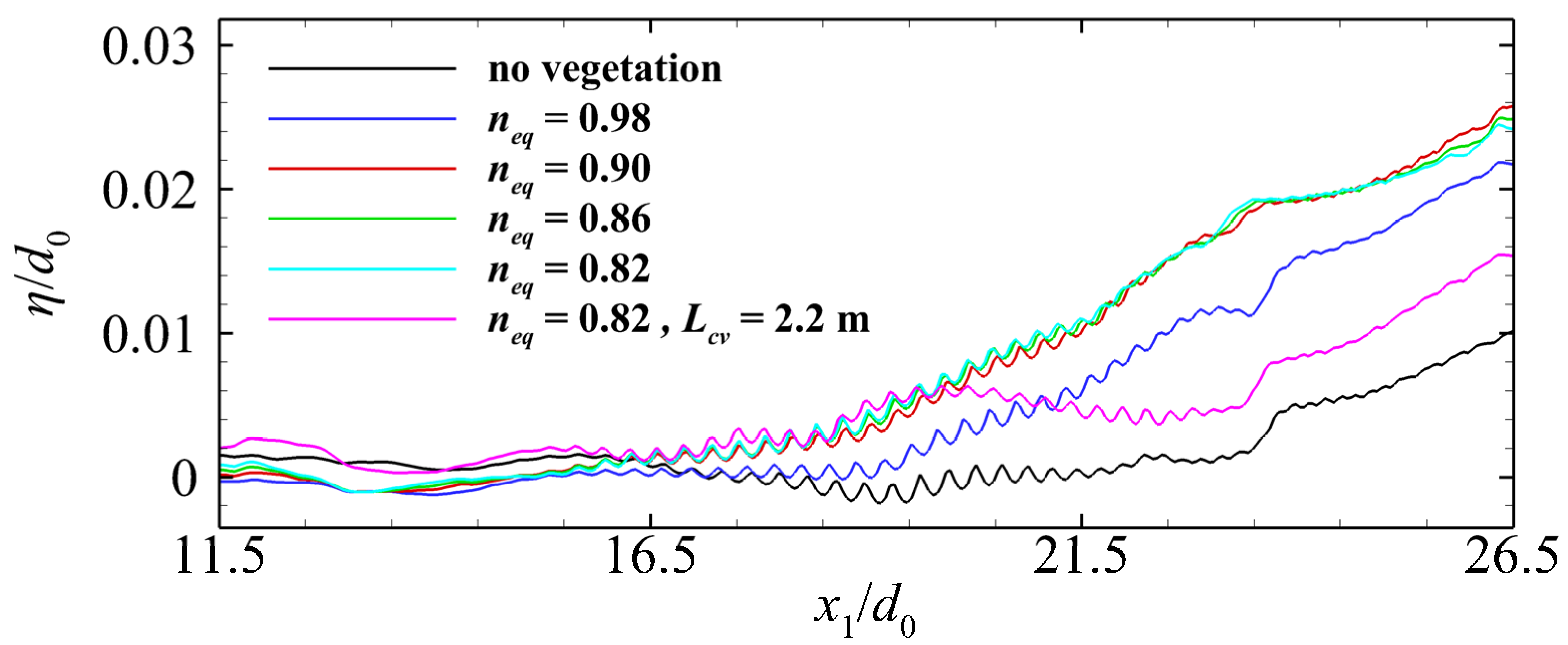
3.4. Phase-Averaged Free-Surface Elevation

The phase-averaged envelope of the free-surface elevation is presented in Figure 7 and Figure 8 for all cases except for the one with the smaller LCV (Case 6 that is presented in Figure 9). The wave-breaking position is marked in all cases with a vertical line. The wave envelope in Cases 1 and 2 is almost identical, demonstrating that the porosity value neq = 0.98 does not significantly affect the wave propagation (Figure 7). In fact, breaking is delayed in Case 2 in comparison to Case 1, and the breaking depth is reduced by about 14%.
Further decrease of neq (Cases 3–5 in Figure 8) causes wave breaking to occur more offshore than the non-vegetation situation (Case 1). Specifically, in Table 2, the wave-breaking characteristics for each case are presented. The wave-breaking height for all cases is approximately the same (largest deviation is about 4%), whereas the breaking depth increases with decreasing neq (40% increase for Case 5), apart for Case 2 (highest neq, i.e., close to 1) where wave breaking is slightly delayed. It is postulated that the latter is due to increased wave shoaling over the CV field, which is characterised by very high porosity, as the breaking depth of the non-vegetated situation (Case 1) is towards the onshore end of the CV field. The presence of the vegetation seems to have a minor effect offshore of the CV field; nevertheless, the reflection coefficient, Cr, remains small. Specifically, Cr was computed using the approximation Cr = (HmaxHmin)/(Hmax + Hmin) where Hmax and Hmin are the maximum and minimum wave heights, respectively, obtained from free-surface elevation results in the horizontal bed part of the computational domain. The computed value of the reflection coefficient for the non-vegetated case is Cr = 0.01, a result which agrees with the prediction obtained by the empirical formula Cr = 0.1ξo2 = 0.01 in Battjes [35]. The computed maximum value of the reflection coefficient for the CV cases is Cr = 0.014.
The effect of LCV on wave propagation and breaking is shown in Figure 9, where the envelope of the free-surface elevation is presented for Cases 4 and 5 (Table 1). The effect of LCV on wave propagation and breaking is notable. In Case 6, the position of wave breaking (at x1/d0 ≈ 21.8) is onshore of the corresponding one in Case 5. The wave-breaking height is not affected significantly (difference ~5.5%). It is noted here that the presence of vegetation with short LCV increases wave shoaling until the onshore end of the CV field (x1/d0 ≈ 18.5, in Figure 9-bottom), similar to the effect in Case 2 (larger LCV and higher neq). After this point (x1/d0 ≈ 18.5), the wave propagates practically unaffected by the CV field and breaks at x1/d0 ≈ 21.8.

3.5. Wave-Induced Current and Wave Setup

The period-mean velocity field, based on the last 10 wave periods of simulations, is compared between Cases 1 and 5 in Figure 10, which is zoomed in the CV area. The undertow current is noticeable in the surf zones of both cases. The distribution of the undertow velocities is strongly modified by the presence of the CV field. Specifically, these velocities in the surf zone shoreward of the CV field are larger (as high as 150% increase) for the non-vegetated case, while, in the area of the CV field, they are larger (as high as 50% increase) for the vegetated Case 5. Inside the vegetation, no noticeable current exists, while even at a distance of about 0.05 d0 above the vegetation field, the undertow current strength is significantly reduced. On the contrary, for the beach with no vegetation, the undertow reaches practically the seabed. It was found that as the vegetation porosity increases, the undertow intensity tends to decrease.
Finally, the period-mean free-surface level for all cases was computed (Figure 11). During the wave shoaling process (up to x1/d0 ≈ 15 depending on the case), the wave setup is almost zero. Small oscillations are observed in the region of wave breaking and surf zone that are due to the small sampling number of averaging (10 waves). The breaking point marks an ascending behaviour of the mean free-surface level, i.e., wave setup. An interesting aspect is that for the cases with 0.82 ≤ neq ≤ 0.90 and the same LCV, the wave setup distribution is practically the same and with values always larger than the ones for the non-vegetated case. The same wave setup behaviour is also observed in Case 6, but its increase is interrupted after the onshore end of the shorter LCV of this case.
In contrast, Case 2 (neq = 0.98) has a higher wave setup than the case with no vegetation but lower than the other cases with the same LCV. The finding of the higher wave setup is important as it highlights that a CV field may also have some negative consequences to the coast, i.e., larger inundation areas. Hence, using vegetation as a coastal protection method should be done with great attention to avoid increasing coastal flooding vulnerability.
In Table 3, the values of the wave setup at the still-water coastline, the wave runup and the x1-coordinate of the seaward boundary of the swash zone are shown for each case. The landward boundary of the swash zone corresponds to the location of wave runup and the seaward boundary to the location of wave rundown. In an experimental study of a CV field on a beach with constant slope tanβ = 1/20, Manousakas et al. [36] reported that depending on incoming wave conditions, i.e., wave height and period, and vegetation parameters, i.e., submergence, the presence of a CV field may decrease or increase wave runup. For the single combination of wave parameters and vegetation height considered in the present study, the presence of the CV field caused wave runup increase. It is postulated that this increase is due to the increase of the breaking depth and/or the decrease of the undertow current velocity shorewards of the CV field in comparison to the non-vegetated case.

4. Discussion

It is recognised that the present numerical study is based on some modelling simplifications. Natural vegetation is not equally distributed, and its density is far more complicated due to different plant branches and leaves. In the present approach, the vegetation density is uniform, whereas in reality, it is lower at the boundaries of the CV. A more detailed approach will be to simulate vegetation fields with zones of different porosity, e.g., denser in the core of the CV. Moreover, in the present approach, rigid vegetation is considered, so the effect of flexibility on wave attenuation is not taken into account. However, in a natural environment, the vegetation is flexible and oscillates under the action of waves. In order to mimic the interaction between waves and coastal vegetation, the effect of vegetation flexibility should also be investigated [32]. Furthermore, only one Iribarren number case was studied. The selection was based on typical Mediterranean coasts that have CV of Posidonia Oceanica.
However, the advantages of the present model should be also highlighted. Utilising the porous medium approach to model the presence of a vegetated habitat is easily applied on Cartesian grids. The combination of this approach with the IB method results in a substantial increase in both the performance and efficiency of the HPC tools used. Moreover, setting aside the dimensions of the vegetation field (hv and LCV), the calibration of this present model is based on one parameter only, the equivalent porosity neq. Thus, many test cases can be easily reproduced without the limitations encountered in experimental facilities. All in all, since the presented porous medium model was proved to be reliable and efficient, more cases with different incoming wave characteristics, beach slopes and CV parameters can be simulated to better understand the effects of CV fields. It is noted that in the present study, the effect of hv on wave attenuation and breaking was not examined and can be considered in future work.

5. Conclusions

In the present work, the effect of a vegetation field on coastal wave attenuation and breaking was studied numerically. The flow field was resolved by means of LES, and the porous medium approach was utilised to model the effect of CV. A good agreement was observed between the numerical results and findings in the literature, indicating that the present approach is a valid model to study the effect on wave attenuation and breaking of a CV field on a beach bed. Moreover, the effect of two parameters, i.e., equivalent porosity, neq, and cross-shore length, LCV, of the CV field was examined. It was found that decreasing neq moves wave breaking offshore at larger depths, while it does not affect much the breaking height. For very high neq and/or short LCV, wave breaking may occur at depths smaller than the non-vegetated situation due to increased wave shoaling over the corresponding CV fields. Finally, the presence of a CV field modifies the undertow current velocities and increases wave setup in the surf zone; the wave setup increases with increasing LCV.

Author Contributions

Conceptualization, I.A.C., G.A.L. and A.A.D.; methodology, I.A.C., G.A.L. and A.A.D.; software, I.A.C. and G.A.L.; validation, I.A.C. and G.A.L.; formal analysis, I.A.C., G.A.L. and A.A.D.; writing—original draft preparation, I.A.C., G.A.L. and A.A.D.; writing—review and editing, I.A.C., G.A.L. and A.A.D.; visualization, I.A.C. and G.A.L.; supervision, A.A.D.; project administration, A.A.D.; All authors have read and agreed to the published version of the manuscript.

Funding

This research received no external funding.

Institutional Review Board Statement

Not applicable.

Informed Consent Statement

Not applicable.

Data Availability Statement

All numerical data are available; please contact by e-mail adimas@upatras.gr.

Acknowledgments

This research was supported by computational time granted from the Greek Research & Technology Network (GRNET) in the National HPC facility—ARIS—under project ID CoastHPC.

Conflicts of Interest

The authors declare no conflict of interest.

References

  1. Vuik, V.; Jonkman, S.N.; Borsje, B.W.; Suzuki, T. Nature-based flood protection: The efficiency of vegetated foreshores for reducing wave loads on coastal dikes. Coast. Eng. 2016, 116, 42–56. [Google Scholar] [CrossRef] [Green Version]
  2. Salauddin, M.; O’Sullivan, J.; Abolfathi, S.; Dong, S.; Pearson, J. Distribution of Individual Wave Overtopping on a Sloping Structure with a Permeable Foreshore. Int. Conf. Coast. Eng. 2020, 36, 54. [Google Scholar] [CrossRef]
  3. Sánchez-González, J.F.; Sánchez-Rojas, V.; Memos, C.D. Wave attenuation due to Posidonia oceanica meadows. J. Hydraul. Res. 2011, 49, 503–514. [Google Scholar] [CrossRef]
  4. Stratigaki, V.; Manca, E.; Prinos, P.; Losada, I.J.; Lara, J.L.; Sclavo, M.; Amos, C.L.; Cáceres, I.; Sánchez-Arcilla, A. Large-scale experiments on wave propagation over Posidonia oceanica. J. Hydraul. Res. 2011, 49, 31–43. [Google Scholar] [CrossRef]
  5. Koftis, T.; Prinos, P.; Stratigaki, V. Wave damping over artificial Posidonia oceanica meadow: A large-scale experimental study. Coast. Eng. 2013, 73, 71–83. [Google Scholar] [CrossRef]
  6. Blackmar, P.J.; Cox, D.T.; Wu, W.C. Laboratory Observations and Numerical Simulations of Wave Height Attenuation in Heterogeneous Vegetation. J. Waterw. Port Coast. Ocean Eng. 2014, 140, 56–65. [Google Scholar] [CrossRef]
  7. Ozeren, Y.; Wren, D.G.; Wu, W. Experimental Investigation of Wave Attenuation through Model and Live Vegetation. J. Waterw. Port Coast. Ocean Eng. 2014, 140, 04014019. [Google Scholar] [CrossRef]
  8. Anderson, M.E.; Smith, J. Wave attenuation by flexible, idealized salt marsh vegetation. Coast. Eng. 2014, 83, 82–92. [Google Scholar] [CrossRef]
  9. Garzon, J.L.; Maza, M.; Ferreira, C.M.; Lara, J.L.; Losada, I.J. Wave attenuation by Spartina saltmarshes in the Chesapeake Bay under storm surge conditions. J. Geoph. Res. Oceans 2019, 124, 5220–5243. [Google Scholar] [CrossRef]
  10. Kobayashi, N.; Raichlen, A.W.; Asano, T. Wave attenuation by vegetation. J. Waterw. Port Coast. Ocean Eng. 1993, 119, 30–48. [Google Scholar] [CrossRef]
  11. Dalrymple, R.A.; Kirby, J.T.; Hwang, P.A. Wave diffraction due to areas of energy dissipation. J. Waterw. Port Coast. Ocean Eng. 1984, 110, 67–79. [Google Scholar] [CrossRef]
  12. Mendez, F.; Losada, I. An empirical model to estimate the propagation of random breaking and nonbreaking waves over vegetation fields. Coast. Eng. 2004, 51, 103–118. [Google Scholar] [CrossRef]
  13. Karambas, T.; Koftis, T.; Prinos, P. Modeling of nonlinear wave attenuation due to vegetation. J. Coast. Res. 2016, 32, 142–152. [Google Scholar]
  14. Yang, Z.; Tang, J.; Shen, Y. Numerical study for vegetation effects on coastal wave propagation by using nonlinear Boussinesq model. Appl. Ocean Res. 2018, 70, 32–40. [Google Scholar] [CrossRef]
  15. Mattis, S.; Kees, C.; Wei, M.; Dimakopoulos, A.; Dawson, C. Computational model for wave attenuation by flexible vegetation. J. Waterw. Port Coast. Ocean Eng. 2019, 145, 04018033. [Google Scholar] [CrossRef]
  16. Wong, C.Y.H.; Dimakopoulos, A.S.; Trinh, P.H.; Chapman, J.S. Multiple-scales analysis of wave evolution in the presence of rigid vegetation. J. Fluid Mech. 2022, 935, A3. [Google Scholar] [CrossRef]
  17. Hadadpour, S.; Paul, M.; Oumeraci, H. Numerical investigation of wave attenuation by rigid vegetation based on a porous media approach. J. Coast. Res. 2019, 92, 92–100. [Google Scholar] [CrossRef]
  18. Liu, P.L.F.; Pengzhi, L.; Chang, K.; Sakakiyama, T. Numerical modeling of wave interaction with porous structures. J. Waterw. Port Coast. Ocean Eng. 1999, 125, 322–330. [Google Scholar] [CrossRef]
  19. Hsu, T.J.; Sakakiyama, T.; Liu, P. A numerical model for wave motions and turbulence flows in front of a composite breakwater. Coast. Eng. 2002, 46, 25–50. [Google Scholar] [CrossRef]
  20. Dimas, A.A.; Chalmoukis, I.A. An adaptation of the immersed boundary method for turbulent flows over three-dimensional coastal/fluvial beds. Appl. Math. Model. 2020, 88, 905–915. [Google Scholar] [CrossRef]
  21. Lesieur, M.; Metais, O. New Trends in Large-Eddy Simulations of Turbulence. Annu. Rev. Fluid Mech. 1996, 28, 45–82. [Google Scholar] [CrossRef]
  22. Rodi, W. Comparison of LES and RANS calculations of the flow around bluff bodies. J. Wind Eng. Ind. Aerodyn. 1997, 69–71, 55–75. [Google Scholar] [CrossRef]
  23. Smagorinsky, J. General circulation experiments with the primitive equations I. The basic experiment. Mon. Weather Rev. 1963, 91, 99–165. [Google Scholar] [CrossRef]
  24. Van Driest, E.R. On turbulent flow near a wall. J. Aeronaut. Sci. 1956, 23, 1007–1011. [Google Scholar] [CrossRef]
  25. Koutrouveli, T.I.; Dimas, A.A. Wave and hydrodynamic processes in the vicinity of a rubble-mound, permeable, zero-freeboard breakwater. J. Mar. Sci. Eng. 2020, 8, 206. [Google Scholar] [CrossRef] [Green Version]
  26. Van Gent, M.R.A. Wave Interaction with Permeable Coastal Structures. Ph.D. Thesis, Delft University, Delft, The Netherlands, 1995. [Google Scholar]
  27. Yang, J.; Stern, F. Sharp interface immersed-boundary/level-set method for wave–body interactions. J. Comput. Phys. 2009, 228, 6590–6616. [Google Scholar] [CrossRef]
  28. Jacobsen, N.G.; Fuhrman, R.; Fredsøe, J. A wave generation toolbox for the open-source CFD library: OpenFoam®. Int. J. Num. Methods Fluids 2012, 70, 1073–1088. [Google Scholar] [CrossRef]
  29. Leftheriotis, G.A.; Chalmoukis, I.A.; Oyarzun, A.G.; Dimas, A.A. A Hybrid Parallel Numerical Model for Wave-Induced Free-Surface Flow. Fluids 2021, 6, 350. [Google Scholar] [CrossRef]
  30. Oyarzun, A.G.; Chalmoukis, I.A.; Leftheriotis, G.A.; Dimas, A.A. A GPU-based algorithm for efficient LES of high Reynolds number flows in heterogeneous CPU/GPU supercomputers. Appl. Math. Model. 2020, 85, 141–156. [Google Scholar] [CrossRef]
  31. Augustin, L.N.; Irish, J.L.; Lynett, P. Laboratory and numerical studies of wave damping by emergent and near-emergent wetland vegetation. Coast. Eng. 2009, 56, 332–340. [Google Scholar] [CrossRef]
  32. Hu, J.; Mei, C.C.; Chang, C.W.; Liu, P.L.F. Effect of flexible coastal vegetation on waves in water of intermediate depth. Coast. Eng. 2021, 168, 103937. [Google Scholar] [CrossRef]
  33. Bouma, T.J.; de Vries, M.B.; Low, E.; Peralta, G.; Tánczos, I.C.; van de Koppel, J.; Herman, P.M.J. Trade-offs related to ecosystem engineering: A case study on stiffness of emerging macrophytes. Ecology 2005, 86, 2187–2199. [Google Scholar] [CrossRef] [Green Version]
  34. Keimer, K.; Schürenkamp, D.; Miescke, F.; Kosmalla, V.; Lojek, O.; Goseberg, N. Ecohydraulics of Surrogate Salt Marshes for Coastal Protection: Wave–Vegetation Interaction and Related Hydrodynamics on Vegetated Foreshores at Sea Dikes. J. Waterw. Port Coast. Ocean Eng. 2021, 147, 04021035. [Google Scholar] [CrossRef]
  35. Battjes, J.A. Surf similarity. In Proceedings of the 14th Coastal Engineering Conference, Copenhagen, Denmark, 24–28 June 1974; pp. 466–480. [Google Scholar]
  36. Manousakas, M.; Salauddin, M.; Pearson, J.; Denissenko, P.; Williams, H.; Abolfathi, S. Effects of Seagrass Vegetation on Wave Runup Reduction—A Laboratory Study. IOP Conf. Ser. Earth Environ. Sci. 2022, 1072, 012004. [Google Scholar] [CrossRef]
Figure 1. Sketch of the configuration of the computational domain with a CV field.
Jmse 11 00519 g001
Figure 2. Experimental setup replicated for the validation of the numerical model. Note that the axes are not in scale for clarity of the exposition.
Jmse 11 00519 g002
Figure 3. Numerical result of the free-surface elevation along with the corresponding experimental result in Augustin et al. [31] where H = 12 cm and T = 1.5 s. The vegetation field comprises cylindrical stems of hv = 0.3 m and D = 12 mm with a density 97 stems/m2 (neq = 0.99), Note that the axes are not in scale for clarity of the exposition.
Jmse 11 00519 g003
Figure 4. Instantaneous free-surface elevation for Case 5 after five wave cycles from the beginning of the simulation for three vertical grid spacing values. Note that the axes are not in scale for clarity of the exposition.
Jmse 11 00519 g004
Figure 5. Instantaneous snapshot of streamwise velocity on the free surface of waves propagating over the CV field with neq = 0.82 (Case 5). Note that the coordinate axes are not in scale for clarity of the exposition.
Jmse 11 00519 g005
Figure 6. Instantaneous 2DV snapshots of streamwise velocity induced by waves propagating over CV fields with LCV = 1.66L and different neq (Cases 2–5). Note that the coordinate axes are in scale x1/x3 = 0.2 for clarity of the exposition.
Jmse 11 00519 g006
Figure 7. Phase-averaged 2DV envelope of the free-surface elevation of waves propagating and breaking for Cases 1 (top) and 2 (bottom). Note that the axes are in scale x1/x3 = 0.1 for clarity of the exposition.
Jmse 11 00519 g007
Figure 8. Phase-averaged 2DV envelope of the free-surface elevation of waves propagating and breaking for Cases 3 (top) to 5 (bottom). Note that the axes are in scale x1/x3 = 0.1 for clarity of the exposition.
Jmse 11 00519 g008
Figure 9. Phase-averaged 2DV envelope of the free-surface elevation of waves propagating and breaking over CV fields with neq = 0.82 and different LCV (Case 5-top and Case 6-bottom). Note that the axes are in scale x1/x3 = 0.1 for clarity of the exposition.
Jmse 11 00519 g009
Figure 10. Period-mean 2DV velocity field (Case 1 on top and Case 5 on bottom). Note that the axes are in scale x1/x3 = 0.3 for clarity of the exposition. The dotted black line indicates the CV area.
Jmse 11 00519 g010
Figure 11. Period-mean free-surface level (wave setup), η ¯ , for all cases. The sloped bed starts at x1/d0 = 11.5, and the still-water coastline is at x1/d0 = 26.5.
Jmse 11 00519 g011
Table 1. Vegetation and wave parameters for all simulated cases.
CaseCVCV Equivalent Porosity (neq)CV Cross-Shore Length (LCV)H (m)T (s)
1noNANA0.181.68
2yes0.985.2 m0.181.68
3yes0.905.2 m0.181.68
4yes0.865.2 m0.181.68
5yes0.825.2 m0.181.68
6yes0.822.6 m0.181.68
Table 2. Wave breaking streamwise position, height and depth for all simulated cases.
CaseneqLCV (m)x1/d0Hb (m)db (m)
1--19.70.200.25
20.985.2 m20.10.190.21
30.905.2 m18.00.170.30
40.865.2 m17.50.170.33
50.825.2 m17.00.180.35
60.822.6 m21.80.160.14
Table 3. Wave setup at the still-water coastline, η ¯ , wave runup, Ru, and x1-coordinate of the seaward boundary of the swash zone, x1s.
CaseneqLCV (m) η ¯ /d0Ru/d0x1s/d0
1--0.0100.03126.62
20.985.2 m0.0210.03926.50
30.905.2 m0.0240.04626.56
40.865.2 m0.0230.04626.55
50.825.2 m0.0230.04326.54
60.822.6 m0.0140.03426.38
Disclaimer/Publisher’s Note: The statements, opinions and data contained in all publications are solely those of the individual author(s) and contributor(s) and not of MDPI and/or the editor(s). MDPI and/or the editor(s) disclaim responsibility for any injury to people or property resulting from any ideas, methods, instructions or products referred to in the content.

