
Coastal Erosion Identification and Monitoring in the Patras Gulf (Greece) Using Multi-Discipline Approaches

 ,
,  , , ,
, , ,  , , ,
, , ,  , and
, and
Abstract
:1. Introduction
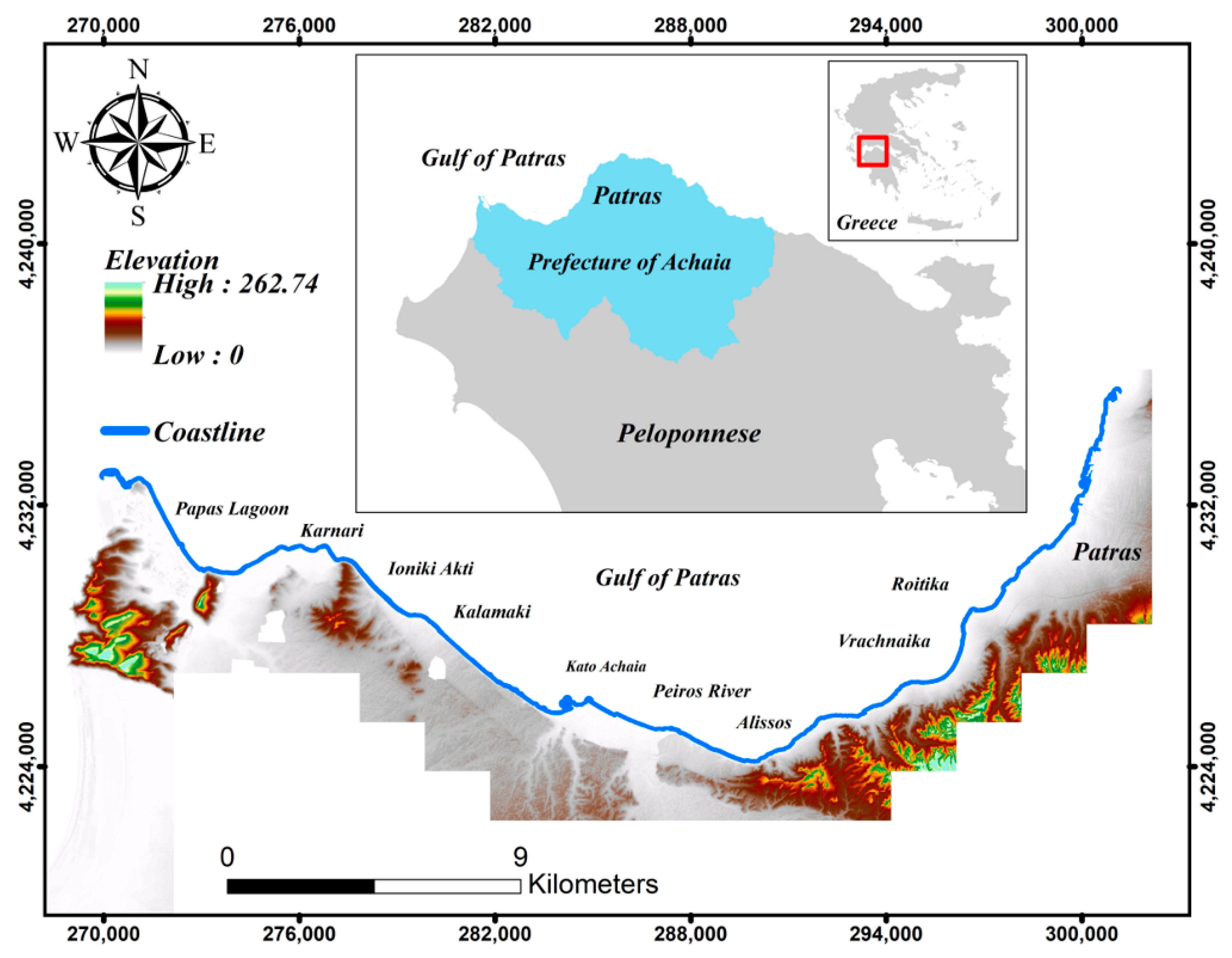
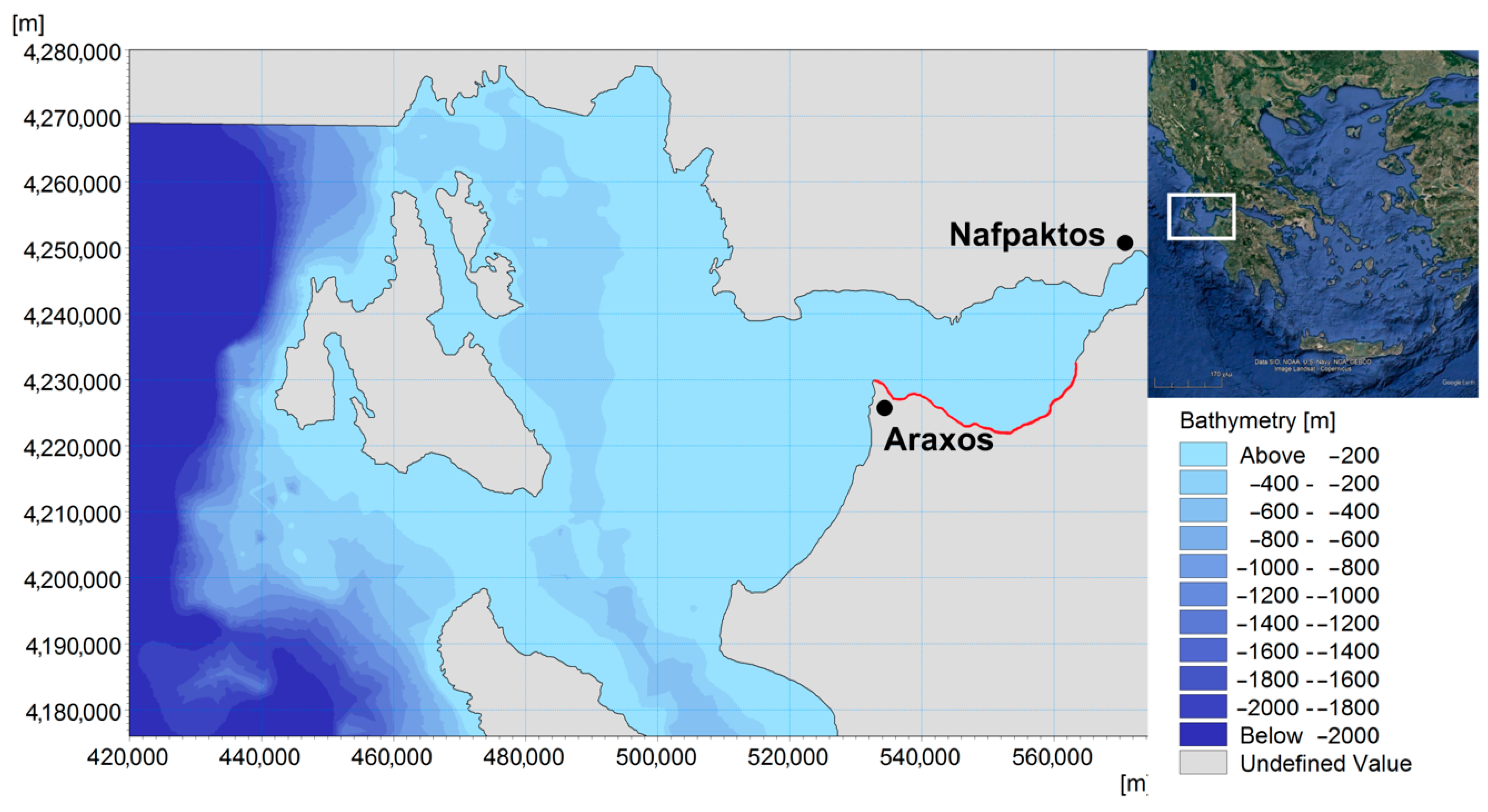
2. Study Area
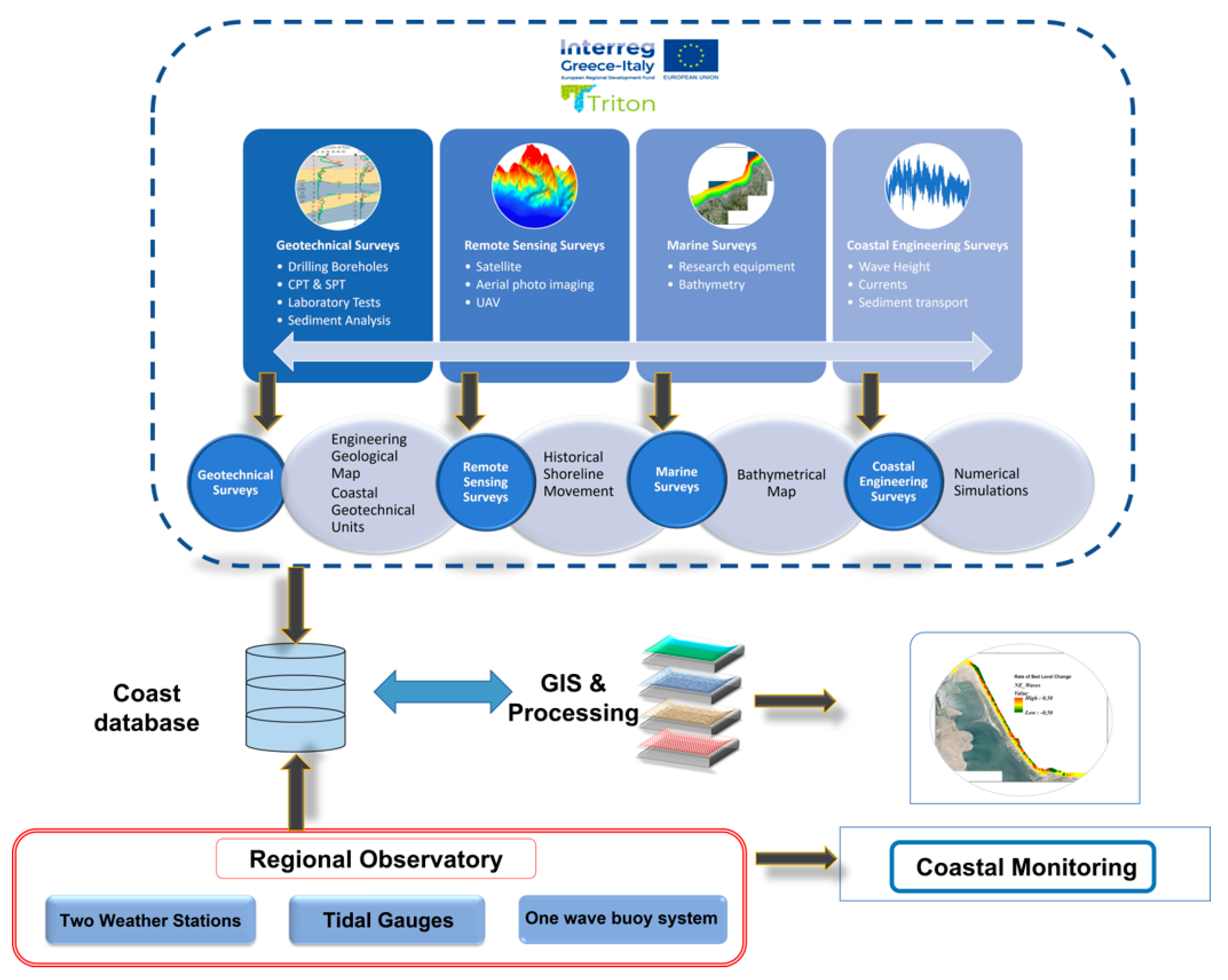
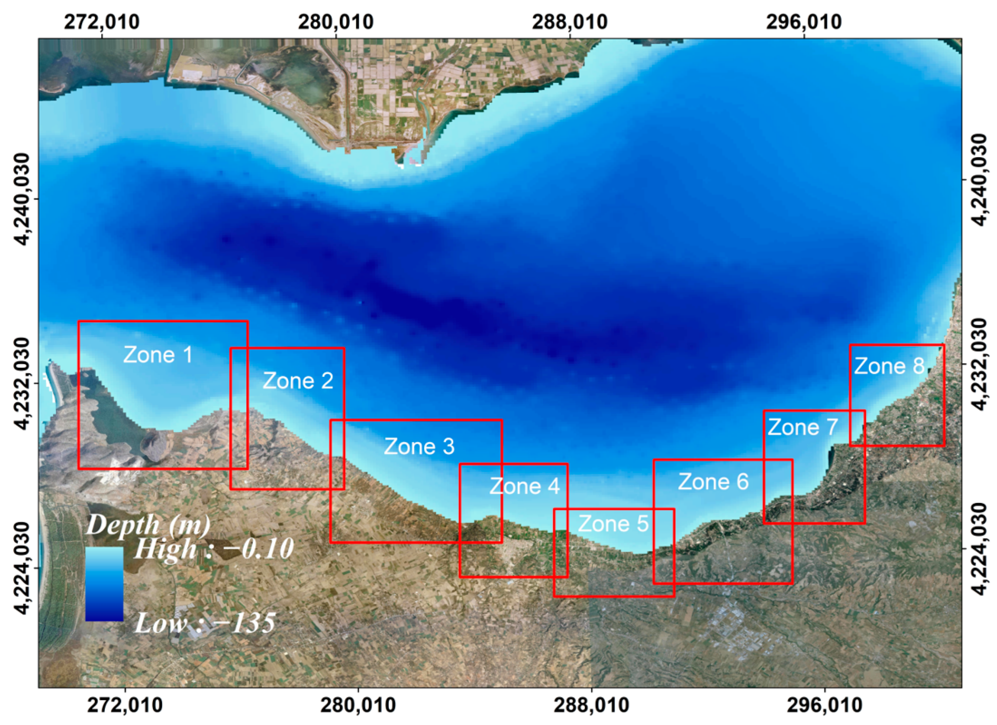
3. Survey Design Plan for Coastal Erosion Identification
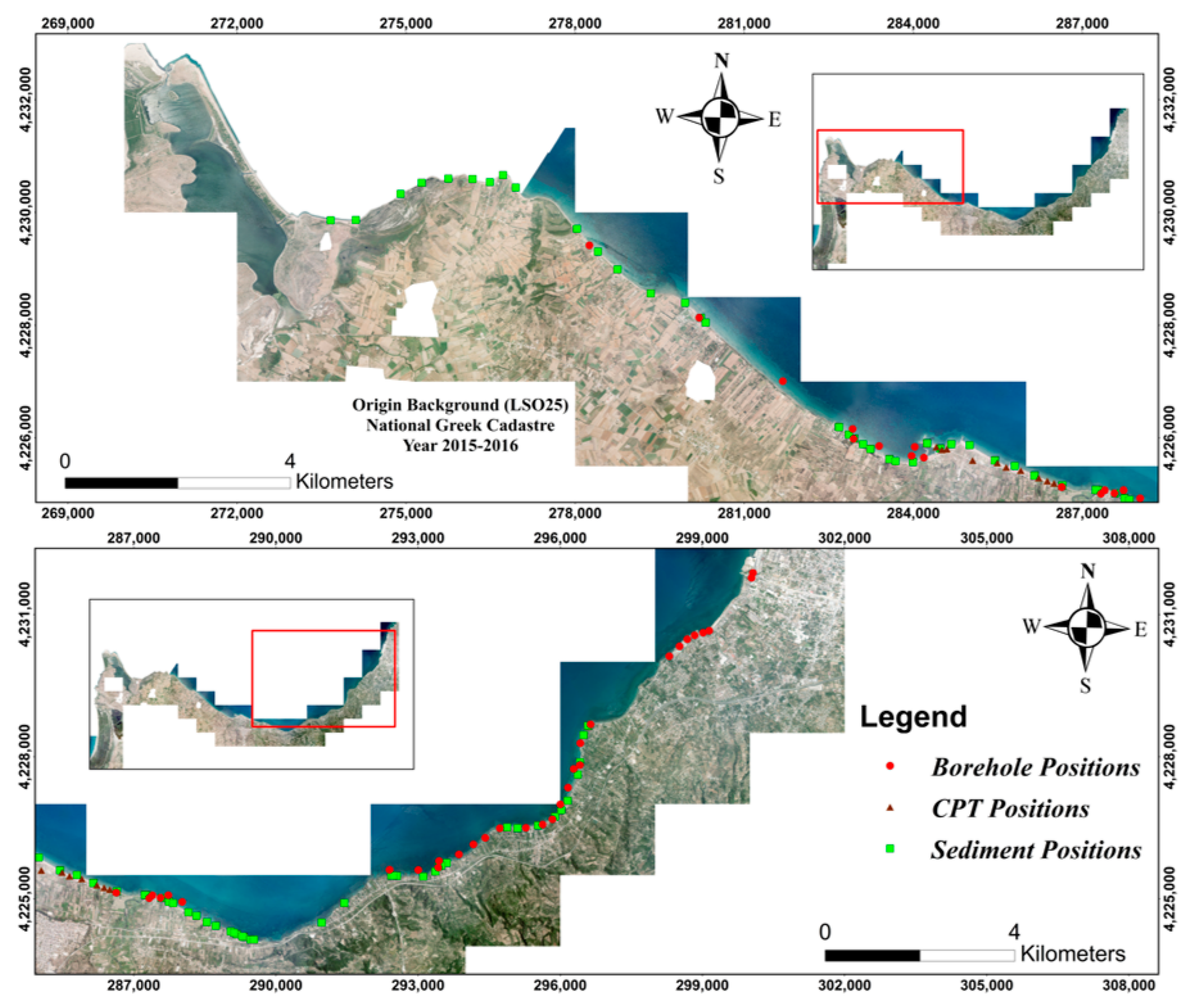
3.1. Geotechnical Surveys
3.2. Remote Sensing Surveys
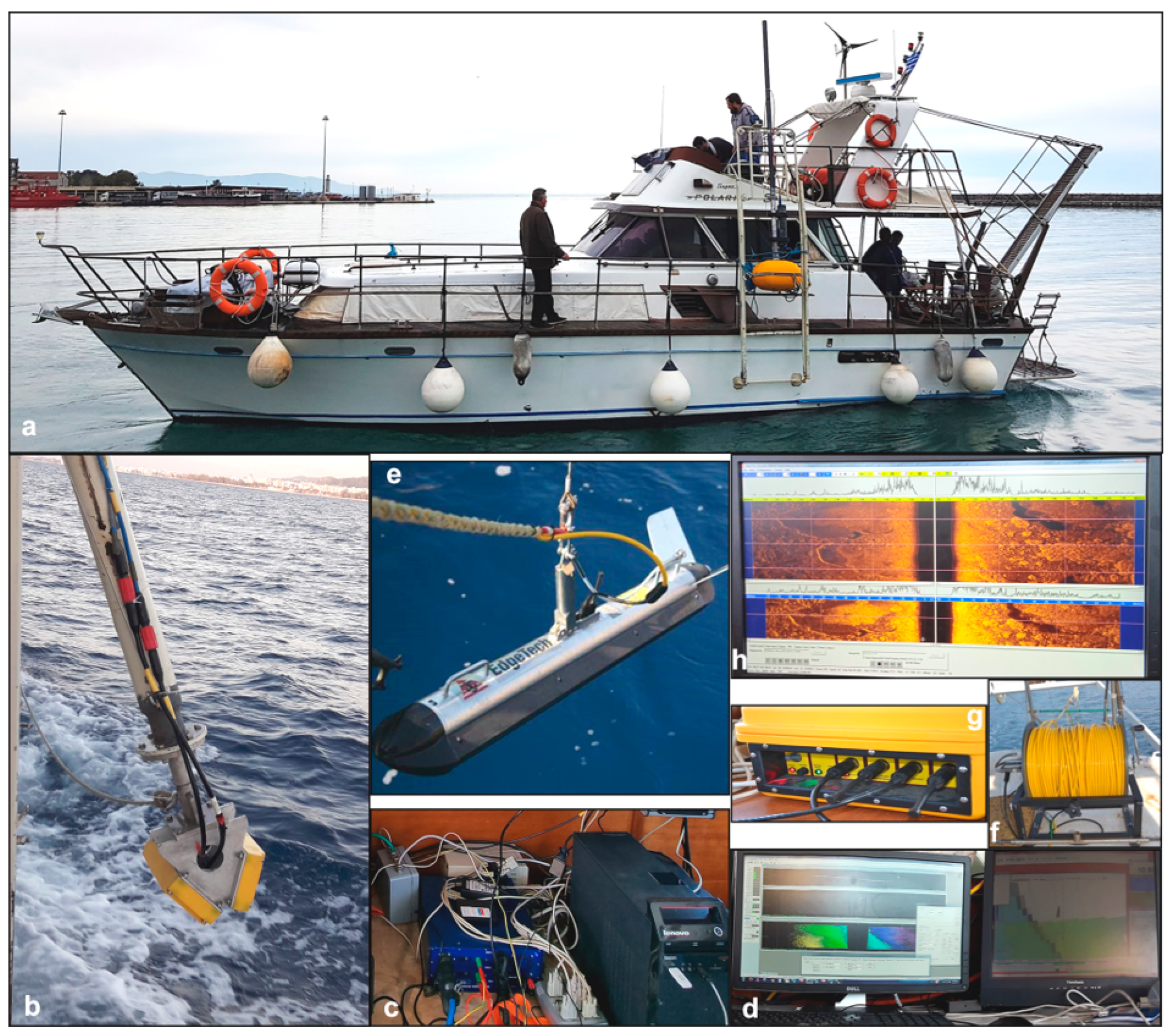
3.3. Marine Survey: Fieldwork and Data Processing
3.3.1. Positioning—Navigation
3.3.2. Bathymetric Survey
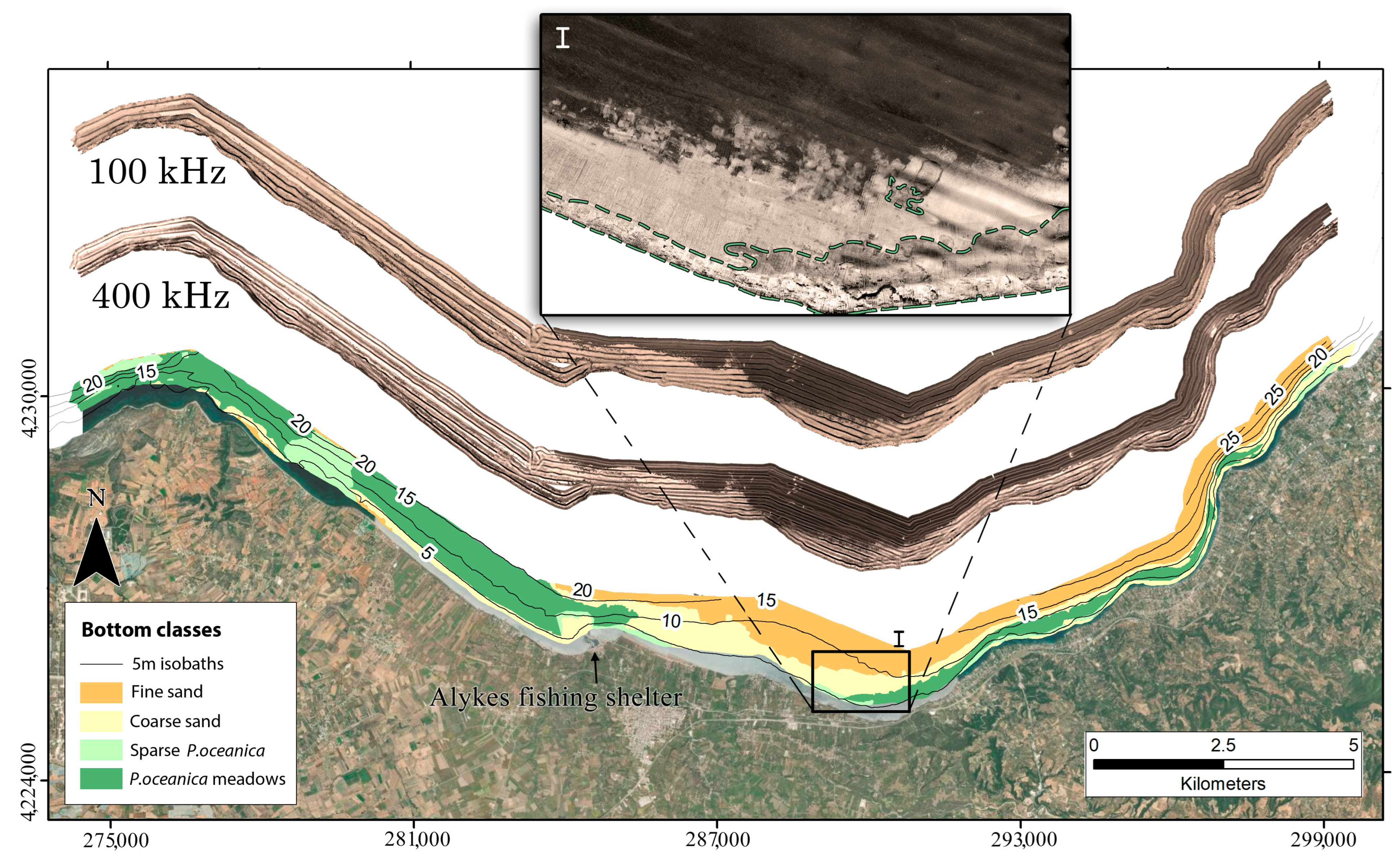
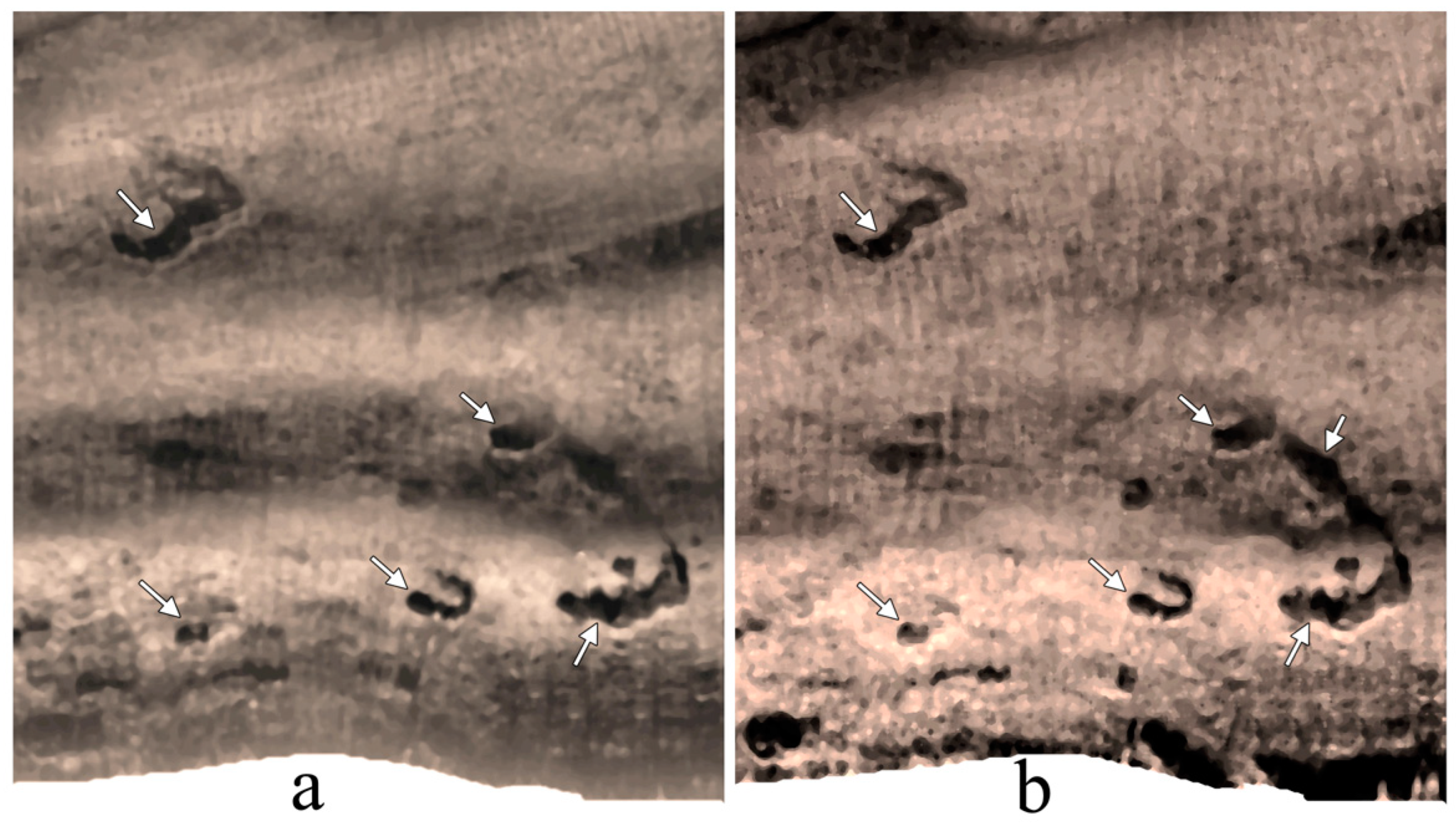
3.3.3. Seabed Morphology Survey
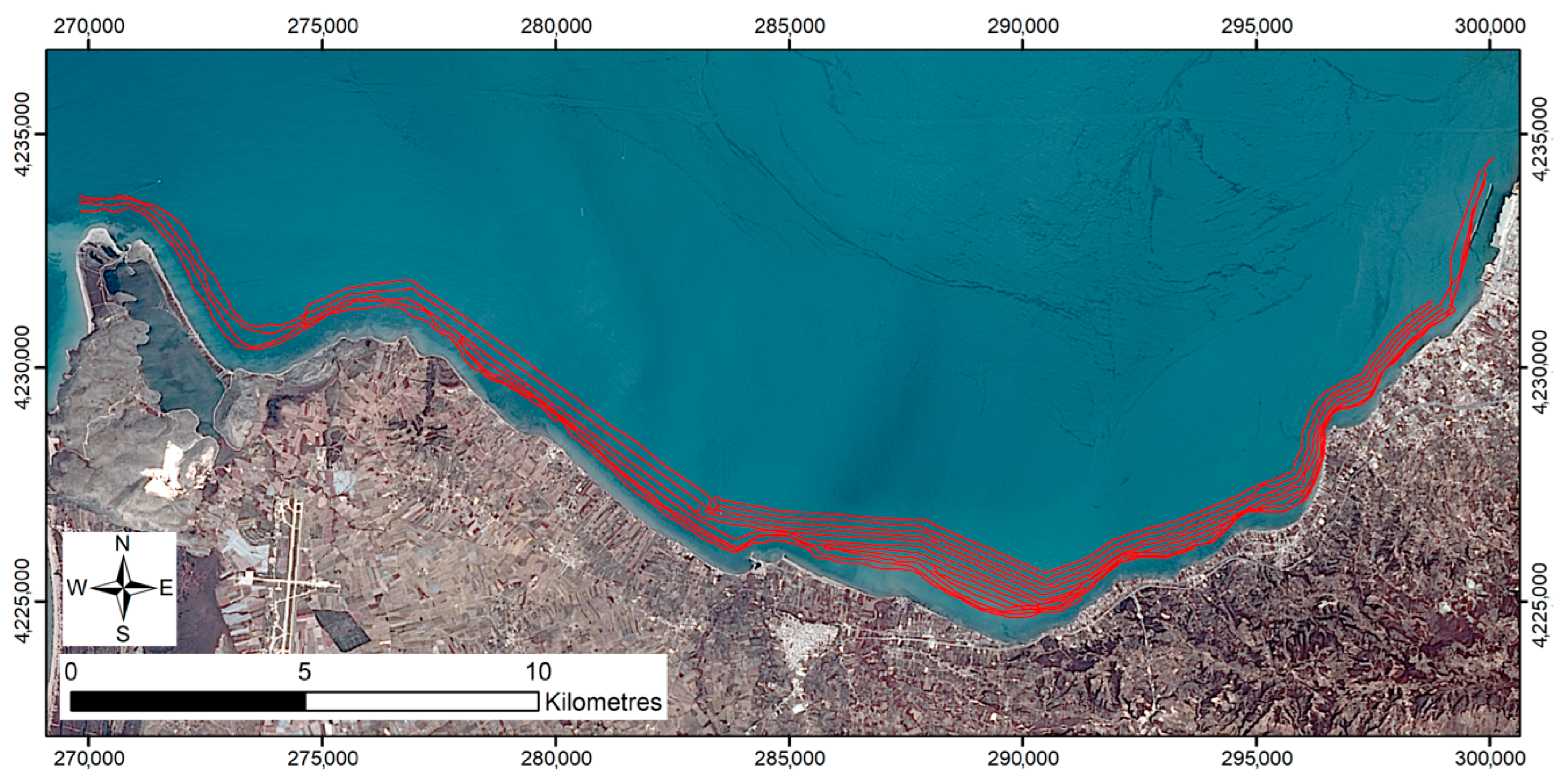
3.3.4. Marine Survey Lines Design
3.4. Coastal Engineering Surveys
- Determination of the deep-water wave parameters due to E, NE, NW, W, and SW winds in the study area.
- Nearshore wave propagation for wind speeds with a return period Tr = 1 year, for each wind direction.
- Nearshore numerical simulation of the magnitude and the direction of the wave-generated currents for each one of the wind cases of stage 2.
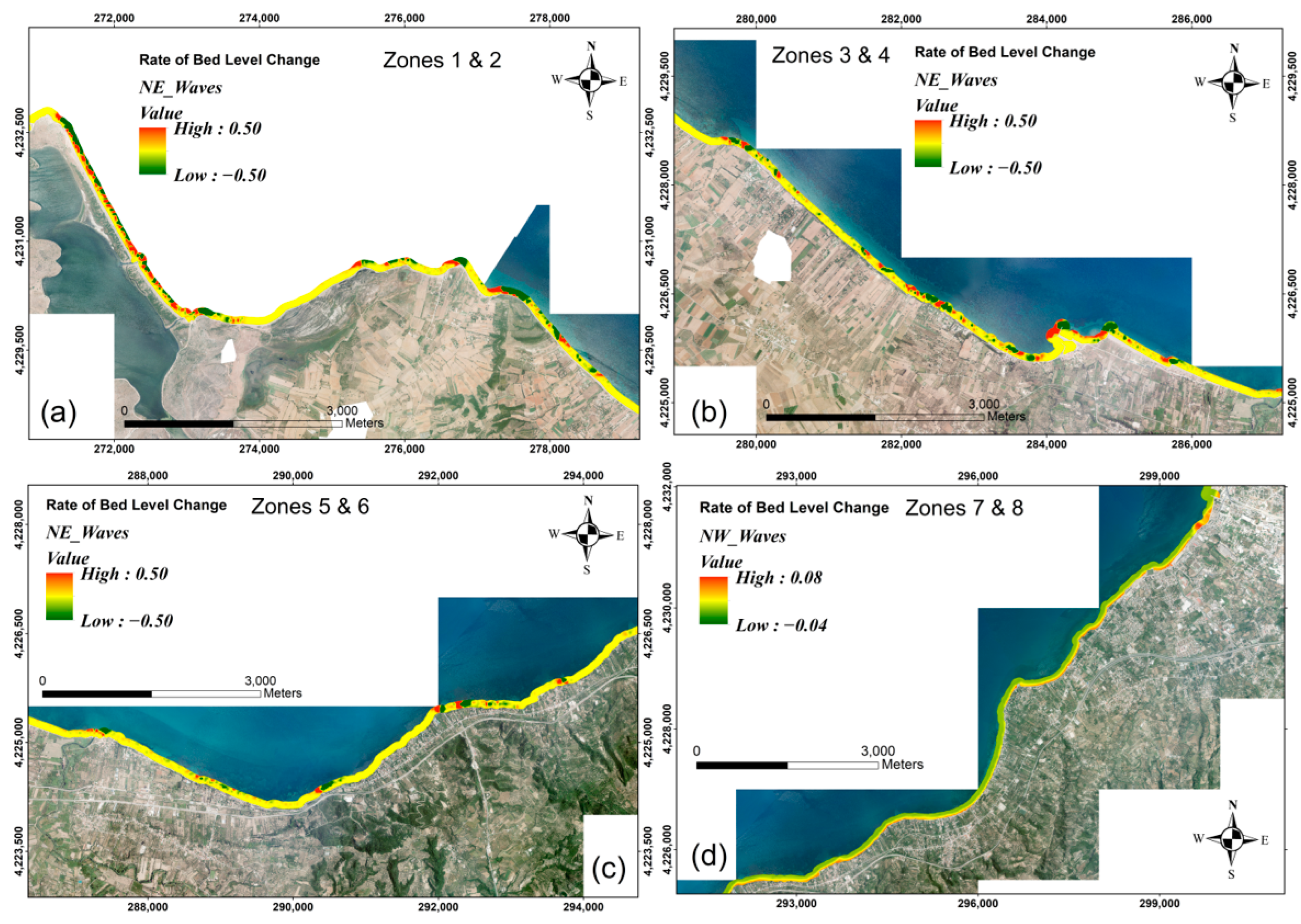
- Numerical simulation of the magnitude and the direction of sediment transport and bed morphodynamic evolution for each one of the wind cases of stage 2.
4. Results
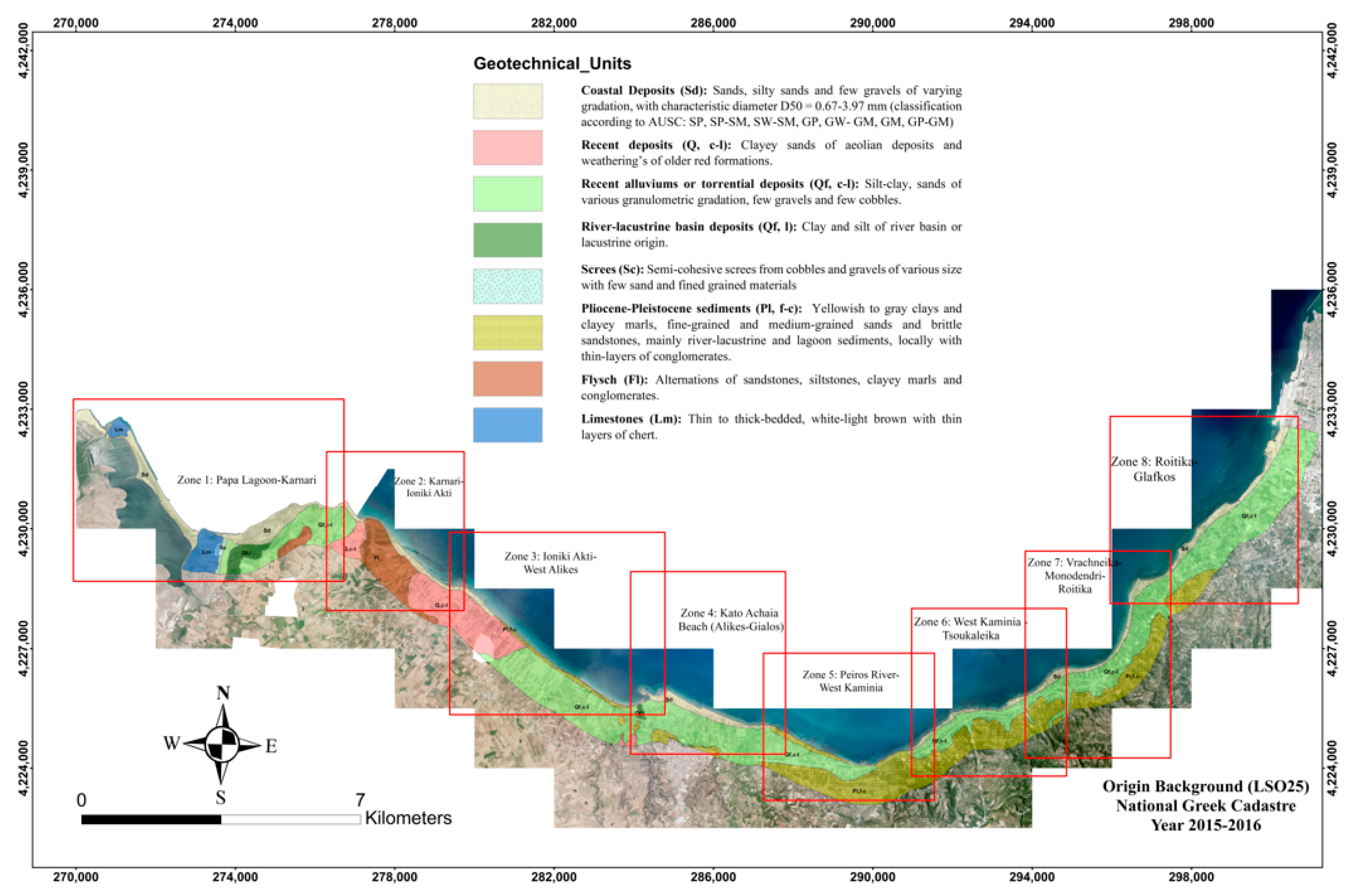
4.1. Engineering Geological Map for Coastal Monitoring
- (1)
- Coastal deposits (Sd): Sands, silty sands, and gravels of varying gradation, with characteristic diameter D50 = 0.67–3.97 mm
- (2)
- Recent deposits (Q, c-l): Clayey sands of aeolian deposits and weatherings of older formations.
- (3)
- Recent alluviums or torrential deposits (Qf, c-l): They consist of silt-clay, sands of various granulometric gradation, few gravels, and cobbles.
- (4)
- River-lacustrine basin deposits (Qf, l): Clay and silt of river or lacustrine origin.
- (5)
- Screes (Sc): Semi-cohesive screes with fine-grained materials.
- (6)
- Pliocene–Pleistocene sediments (Pl, f-c): Yellowish to grey clays and marls, fine and medium-grained sands, brittle sandstones, and river-lacustrine and lagoon sediments.
- (7)
- Flysch (Fl): Sandstones, siltstones, marls, and conglomerates.
- (8)
- Limestones (Lm): Rock formation with thin layers of cherts.
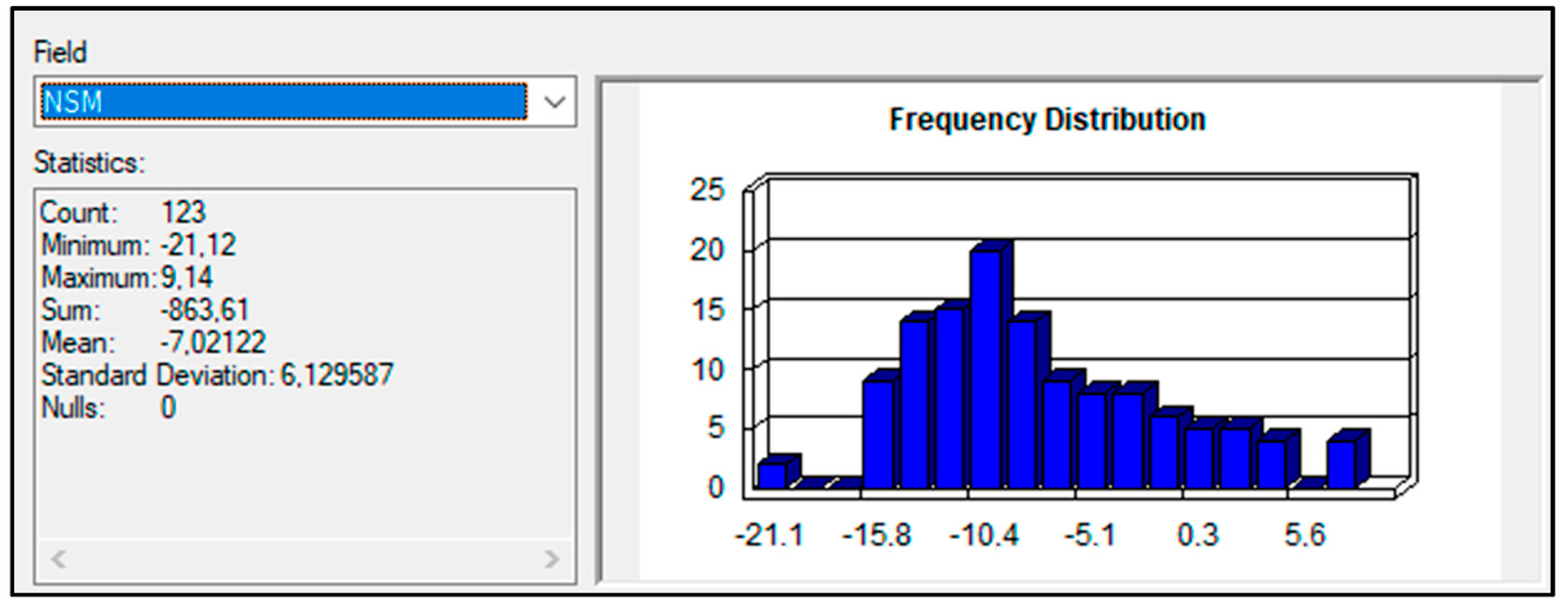
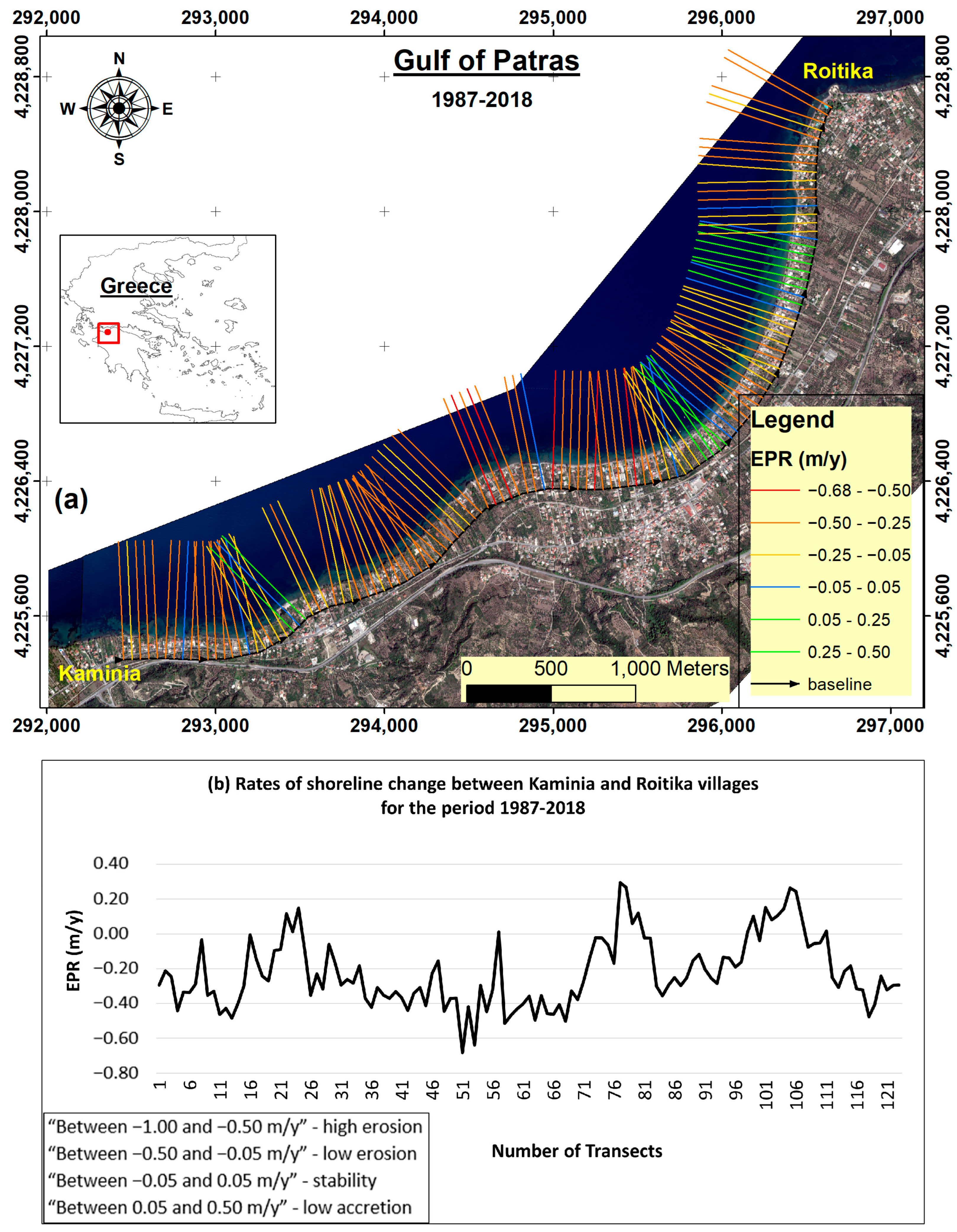
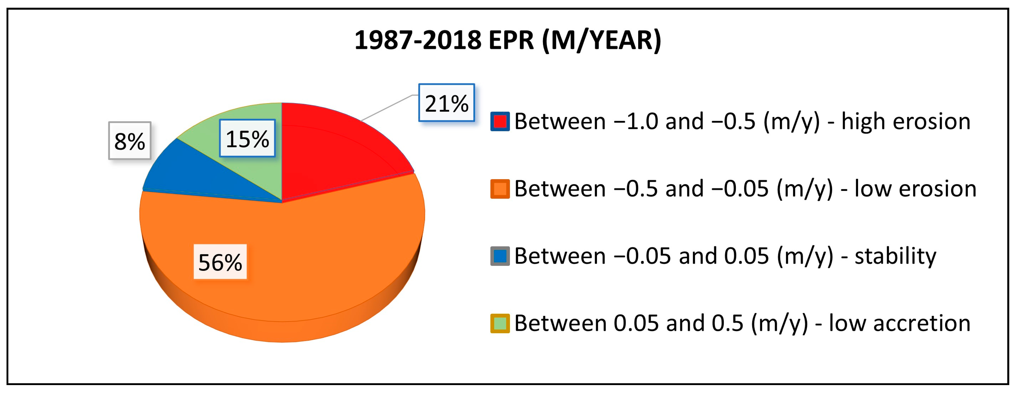
4.2. Orthomosaics and Aerial Photo Imaging Results
- high erosion “Between −1.00 and −0.50 m/y”
- low erosion “Between −0.50 and −0.05 m/y”
- stability “Between −0.05 and 0.05 m/y”
- low accretion “Between 0.05 and 0.50 m/y”
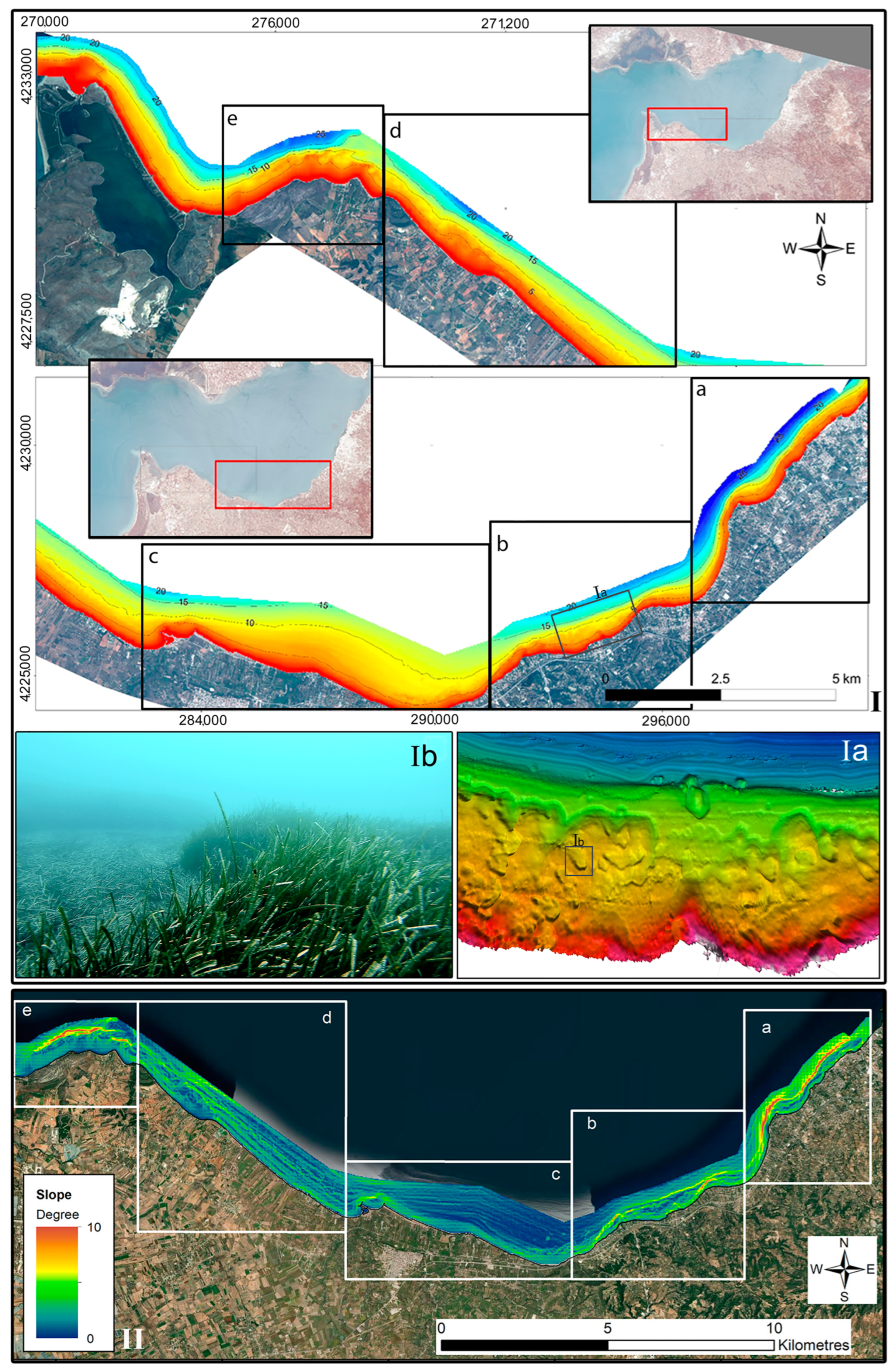
4.3. Digital Bathymetric Plans and Results
4.4. Coastal Engineering Results
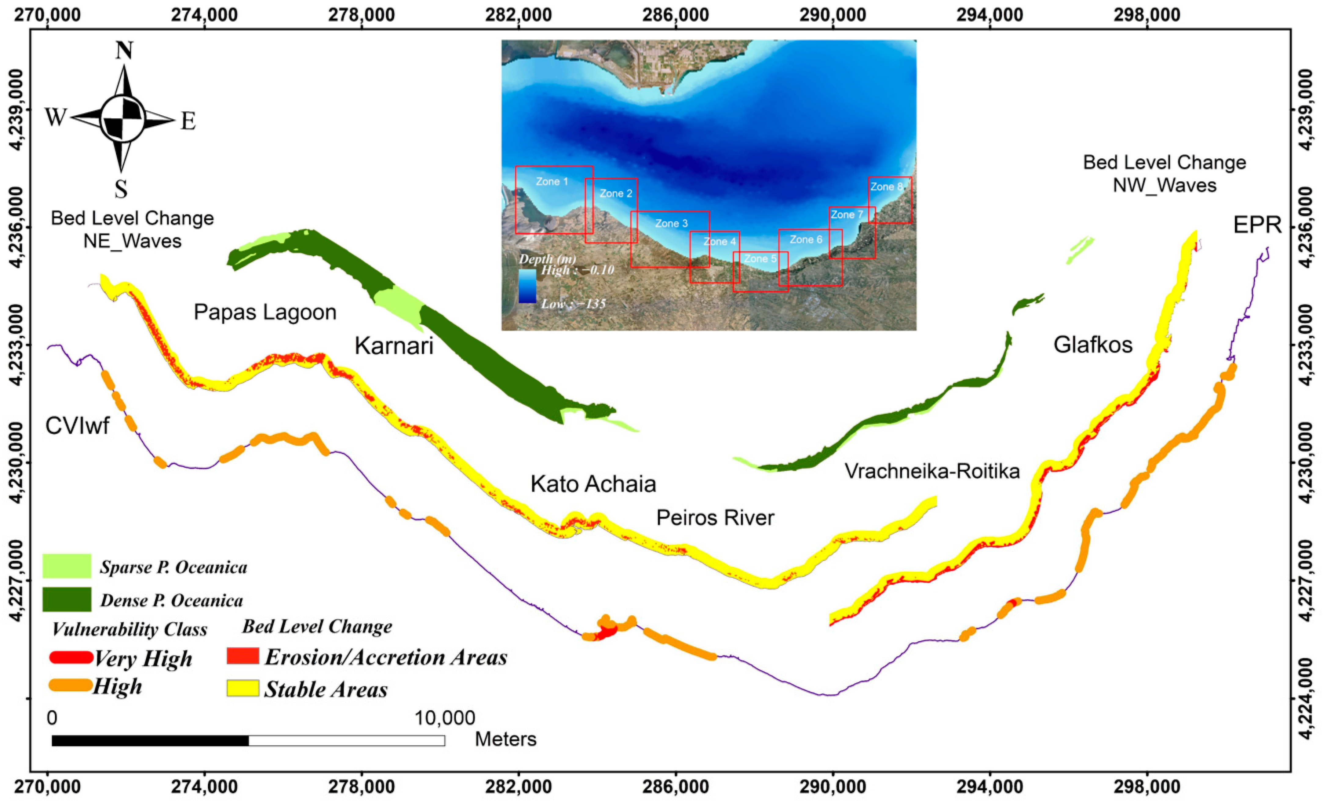
4.5. Coastal Vulnerability Index (CVI)
5. Discussion
6. Conclusions
Author Contributions
Funding
Data Availability Statement
Acknowledgments
Conflicts of Interest
References
- IPCC. Global Warming of 1.5 °C; IPCC: Geneva, Switzerland, 2018; ISBN 9781009157940. [Google Scholar]
- Bunce, M.; Brown, K.; Rosendo, S. Policy Misfits, Climate Change and Cross-Scale Vulnerability in Coastal Africa: How Development Projects Undermine Resilience. Environ. Sci. Policy 2010, 13, 485–497. [Google Scholar] [CrossRef]
- Ferro-Azcona, H.; Espinoza-Tenorio, A.; Calderón-Contreras, R.; Ramenzoni, V.C.; País, M.D.L.M.G.; Mesa-Jurado, M.A. Adaptive Capacity and Social-Ecological Resilience of Coastal Areas: A Systematic Review. Ocean Coast. Manag. 2019, 173, 36–51. [Google Scholar] [CrossRef]
- IPCC. Climate Change 2014 Part A: Global and Sectoral Aspects; IPCC: Geneva, Switzerland, 2014; ISBN 9781107641655. [Google Scholar]
- Carson, M.; Köhl, A.; Stammer, D.; ASlangen, A.B.; Katsman, C.A.; van de Wal, R.S.W.; Church, J.; White, N. Coastal Sea Level Changes, Observed and Projected during the 20th and 21st Century. Clim. Chang. 2016, 134, 269–281. [Google Scholar] [CrossRef]
- van Dongeren, A.; Ciavola, P.; Martinez, G.; Viavattene, C.; Bogaard, T.; Ferreira, O.; Higgins, R.; McCall, R. Introduction to RISC-KIT: Resilience-Increasing Strategies for Coasts. Coast. Eng. 2018, 134, 2–9. [Google Scholar] [CrossRef] [Green Version]
- Gibbs, M.T. Consistency in Coastal Climate Adaption Planning in Australia and the Importance of Understanding Local Political Barriers to Implementation. Ocean Coast. Manag. 2019, 173, 131–138. [Google Scholar] [CrossRef]
- Ramieri, E.; Hartley, A.J.; Barbanti, A.; Santos, F.D.; Gomes, A.; Hilden, M.; Laihonen, P.; Marinova, N.; Santini, M. Methods for Assessing Coastal Vulnerability to Climate Change. Eur. Environ. Agency Eur. Top. Cent. Clim. Chang. Impacts Vulnerability Adapt. 2011, 1–93. [Google Scholar]
- Losada, I.J.; Toimil, A.; Muñoz, A.; Garcia-Fletcher, A.P.; Diaz-Simal, P. A Planning Strategy for the Adaptation of Coastal Areas to Climate Change: The Spanish Case. Ocean Coast. Manag. 2019, 182, 104983. [Google Scholar] [CrossRef]
- Toimil, A.; Losada, I.J.; Nicholls, R.J.; Dalrymple, R.A.; Stive, M.J.F. Addressing the Challenges of Climate Change Risks and Adaptation in Coastal Areas: A Review. Coast. Eng. 2020, 156, 103611. [Google Scholar] [CrossRef]
- Bongarts Lebbe, T.; Rey-Valette, H.; Chaumillon, É.; Camus, G.; Almar, R.; Cazenave, A.; Claudet, J.; Rocle, N.; Meur-Férec, C.; Viard, F.; et al. Designing Coastal Adaptation Strategies to Tackle Sea Level Rise. Front. Mar. Sci. 2021, 8, 1640. [Google Scholar] [CrossRef]
- Gornitz, V. Global Coastal Hazards from Future Sea Level Rise. Palaeogeogr. Palaeoclimatol. Palaeoecol. 1991, 89, 379–398. [Google Scholar] [CrossRef]
- De Serio, F.; Armenio, E.; Mossa, M.; Petrillo, A.F. How to Define Priorities in Coastal Vulnerability Assessment. Geosciences 2018, 8, 415. [Google Scholar] [CrossRef] [Green Version]
- Furlan, E.; Pozza, P.D.; Michetti, M.; Torresan, S.; Critto, A.; Marcomini, A. Development of a Multi-Dimensional Coastal Vulnerability Index: Assessing Vulnerability to Inundation Scenarios in the Italian Coast. Sci. Total Environ. 2021, 772, 144650. [Google Scholar] [CrossRef] [PubMed]
- Hinkel, J.; Klein, R.J.T. Integrating Knowledge to Assess Coastal Vulnerability to Sea-Level Rise: The Development of the DIVA Tool. Glob. Environ. Chang. 2009, 19, 384–395. [Google Scholar] [CrossRef]
- Torresan, S.; Zabeo, A.; Rizzi, J.; Critto, A.; Pizzol, L.; Giove, S.; Marcomini, A. Risk Assessment and Decision Support Tools for the Integrated Evaluation of Climate Change Impacts on Coastal Zones. In Proceedings of the 5th International Congress on Environmental Modelling and Software, Ottawa, ON, Canada, 5–8 July 2010; Volume 3, pp. 2409–2416. [Google Scholar]
- Zanuttigh, B.; Simcic, D.; Bagli, S.; Bozzeda, F.; Pietrantoni, L.; Zagonari, F.; Hoggart, S.; Nicholls, R.J. THESEUS Decision Support System for Coastal Risk Management. Coast. Eng. 2014, 87, 218–239. [Google Scholar] [CrossRef]
- Zennaro, F.; Furlan, E.; Simeoni, C.; Torresan, S.; Aslan, S.; Critto, A.; Marcomini, A. Exploring Machine Learning Potential for Climate Change Risk Assessment. Earth-Sci. Rev. 2021, 220, 103752. [Google Scholar] [CrossRef]
- Harris, R.; Furlan, E.; Pham, H.V.; Torresan, S.; Mysiak, J.; Critto, A. A Bayesian Network Approach for Multi-Sectoral Flood Damage Assessment and Multi-Scenario Analysis. Clim. Risk Manag. 2022, 35, 100410. [Google Scholar] [CrossRef]
- Barco, D.; Pham, H.V.; Fogarin, S.; Zanetti, M.; Harris, R.; Rubinetti, S.; Rubino, A.; Zanchettin, D.; Barbariol, F.; Benetazzo, A.; et al. Evaluating Climate Change and Coastal Erosion Risks on the Venice Coastline: A Machine Learning Approach Supporting Multi-Risk Scenario Analysis. In Proceedings of the EGU General Assembly Conference Abstracts, Vienna, Austria, 3–27 May 2022. [Google Scholar]
- Environment Agency. Maritime Local Authorities the Coastal Handbook: A Guide for All Those Working on the Coast. Environ. Agency Marit. Local Authorities 2010, 220. [Google Scholar]
- Becker, A.; Brown, J.; Bricheno, L.; Wolf, J. Guidance Note on the Application of Coastal Monitoring for Small Island Developing States. 2020. Available online: https://www.cmeprogramme.org/sites/cme-programme/files/documents/reports/Becker_et_al_NOC_R&C_74_2020.pdf (accessed on 7 January 2023).
- Kerguillec, R.; Audère, M.; Baltzer, A.; Debaine, F.; Fattal, P.; Juigner, M.; Launeau, P.; Le Mauff, B.; Luquet, F.; Maanan, M.; et al. Monitoring and Management of Coastal Hazards: Creation of a Regional Observatory of Coastal Erosion and Storm Surges in the Pays de La Loire Region (Atlantic Coast, France). Ocean Coast. Manag. 2019, 181, 104904. [Google Scholar] [CrossRef]
- Bio, A.; Bastos, L.; Granja, H.; Pinho, J.L.S.; Goncalves, J.A.; Henriques, R.; Madeira, S.; Magalhaes, A.; Rodrigues, D. Methods for Coastal Monitoring and Erosion Risk Assessment: Two Portuguese Case Studies. J. Integr. Coast. Zo. Manag. 2015, 15, 47–63. [Google Scholar] [CrossRef] [Green Version]
- Romagnoli, C.; Sistilli, F.; Cantelli, L.; Aguzzi, M.; De Nigris, N.; Morelli, M.; Gaeta, M.G.; Archetti, R. Beach Monitoring and Morphological Response in the Presence of Coastal Defense Strategies at Riccione (Italy). J. Mar. Sci. Eng. 2021, 9, 851. [Google Scholar] [CrossRef]
- Almonacid-Caballer, J.; Sánchez-García, E.; Pardo-Pascual, J.E.; Balaguer-Beser, A.A.; Palomar-Vázquez, J. Evaluation of Annual Mean Shoreline Position Deduced from Landsat Imagery as a Mid-Term Coastal Evolution Indicator. Mar. Geol. 2016, 372, 79–88. [Google Scholar] [CrossRef]
- Almeida, L.P.; Almar, R.; Bergsma, E.W.J.; Berthier, E.; Baptista, P.; Garel, E.; Dada, O.A.; Alves, B. Deriving High Spatial-Resolution Coastal Topography from Sub-Meter Satellite Stereo Imagery. Remote Sens. 2019, 11, 590. [Google Scholar] [CrossRef] [Green Version]
- Hodúl, M.; Bird, S.; Knudby, A.; Chénier, R. Satellite Derived Photogrammetric Bathymetry. ISPRS J. Photogramm. Remote Sens. 2018, 142, 268–277. [Google Scholar] [CrossRef]
- Turner, I.L.; Harley, M.D.; Almar, R.; Bergsma, E.W.J. Satellite Optical Imagery in Coastal Engineering. Coast. Eng. 2021, 167, 103919. [Google Scholar] [CrossRef]
- Brock, J.C.; Purkis, S.J. The Emerging Role of Lidar Remote Sensing in Coastal Research and Resource Management. J. Coast. Res. 2009, 10053, 1–5. [Google Scholar] [CrossRef]
- Young, A.P.; Olsen, M.J.; Driscoll, N.; Rick, R.E.; Gutierrez, R.; Guza, R.T.; Johnstone, E.; Kuester, F. Comparison of Airborne and Terrestrial Lidar Estimates of Seacliff Erosion in Southern California. Photogramm. Eng. Remote Sensing 2010, 76, 421–427. [Google Scholar] [CrossRef] [Green Version]
- Klemas, V. Beach Profiling and LIDAR Bathymetry: An Overview with Case Studies. J. Coast. Res. 2011, 27, 1019–1028. [Google Scholar] [CrossRef]
- O’Dea, A.; Brodie, K.L.; Hartzell, P. Continuous Coastal Monitoring with an Automated Terrestrial Lidar Scanner. J. Mar. Sci. Eng. 2019, 7, 37. [Google Scholar] [CrossRef] [Green Version]
- Nikolakopoulos, K.G.; Lampropoulou, P.; Fakiris, E.; Sardelianos, D.; Papatheodorou, G. Synergistic Use of UAV and USV Data and Petrographic Analyses for the Investigation of Beachrock Formations: A Case Study from Syros Island, Aegean Sea, Greece. Minerals 2018, 8, 534. [Google Scholar] [CrossRef] [Green Version]
- Archetti, R.; Zanuttigh, B. Integrated Monitoring of the Hydro-Morphodynamics of a Beach Protected by Low Crested Detached Breakwaters. Coast. Eng. 2010, 57, 879–891. [Google Scholar] [CrossRef]
- Uunk, L.; Wijnberg, K.M.; Morelissen, R. Automated Mapping of the Intertidal Beach Bathymetry from Video Images. Coast. Eng. 2010, 57, 461–469. [Google Scholar] [CrossRef]
- Almar, R.; Bergsma, E.W.J.; Maisongrande, P.; de Almeida, L.P.M. Wave-Derived Coastal Bathymetry from Satellite Video Imagery: A Showcase with Pleiades Persistent Mode. Remote Sens. Environ. 2019, 231, 111263. [Google Scholar] [CrossRef]
- Apostolopoulos, D.N.; Nikolakopoulos, K.G. Synergy of UAV Data and in Situ Measurements for the Shoreline Mapping in Arkoudi Beach, Western Greece. In Earth Resources and Environmental Remote Sensing/GIS Applications XIII; SPIE: Bellingham, WA, USA, 2022; Volume 12268, pp. 244–256. [Google Scholar] [CrossRef]
- Nikolakopoulos, K.; Kyriou, A.; Koukouvelas, I.; Zygouri, V.; Apostolopoulos, D. Combination of Aerial, Satellite, and UAV Photogrammetry for Mapping the Diachronic Coastline Evolution: The Case of Lefkada Island. ISPRS Int. J. Geo-Inf. 2019, 8, 489. [Google Scholar] [CrossRef] [Green Version]
- Viaña-Borja, S.P.; Ortega-Sánchez, M. Automatic Methodology to Detect the Coastline from Landsat Images with a New Water Index Assessed on Three Different Spanish Mediterranean Deltas. Remote Sens. 2019, 11, 2186. [Google Scholar] [CrossRef] [Green Version]
- McFeeters, S.K. The Use of the Normalized Difference Water Index (NDWI) in the Delineation of Open Water Features. Int. J. Remote Sens. 1996, 17, 1425–1432. [Google Scholar] [CrossRef]
- Xu, H. Modification of Normalised Difference Water Index (NDWI) to Enhance Open Water Features in Remotely Sensed Imagery. Int. J. Remote Sens. 2006, 27, 3025–3033. [Google Scholar] [CrossRef]
- Feyisa, G.L.; Meilby, H.; Fensholt, R.; Proud, S.R. Automated Water Extraction Index: A New Technique for Surface Water Mapping Using Landsat Imagery. Remote Sens. Environ. 2014, 140, 23–35. [Google Scholar] [CrossRef]
- Baily, B.; Nowell, D. Techniques for Monitoring Coastal Change: A Review and Case Study. Ocean Coast. Manag. 1996, 32, 85–95. [Google Scholar] [CrossRef]
- Boak, E.H.; Turner, I.L. Shoreline Definition and Detection: A Review. J. Coast. Res. 2005, 21, 688–703. [Google Scholar] [CrossRef] [Green Version]
- Apostolopoulos, D.; Nikolakopoulos, K. A Review and Meta-Analysis of Remote Sensing Data, GIS Methods, Materials and Indices Used for Monitoring the Coastline Evolution over the Last Twenty Years. Eur. J. Remote Sens. 2021, 54, 240–265. [Google Scholar] [CrossRef]
- Fakiris, E.; Blondel, P.; Papatheodorou, G.; Christodoulou, D.; Dimas, X.; Georgiou, N.; Kordella, S.; Dimitriadis, C.; Rzhanov, Y.; Geraga, M.; et al. Multi-Frequency, Multi-Sonar Mapping of Shallow Habitats-Efficacy and Management Implications in the National Marine Park of Zakynthos, Greece. Remote Sens. 2019, 11, 461. [Google Scholar] [CrossRef] [Green Version]
- Pasqualini, V.; Pergent-Martini, C.; Pergent, G. Use of Remote Sensing for the Characterization of the Mediterranean Coastal Environment—The Case of Posidonia Oceanica. J. Coast. Conserv. 1998, 4, 59–66. [Google Scholar] [CrossRef]
- Duarte, C.M. Seagrass Depth Limits. Aquat. Bot. 1991, 40, 363–377. [Google Scholar] [CrossRef]
- Terrados, J.; Duarte, C.M. Experimental Evidence of Reduced Particle Resuspension within a Seagrass (Posidonia Oceanica L.) Meadow. J. Exp. Mar. Bio. Ecol. 2000, 243, 45–53. [Google Scholar] [CrossRef]
- Boudouresque, C.F.; Meinesz, A. Découverte de l’herbier de Posidonie. Cah. Parc Nation 1982, 4, 1–79. [Google Scholar]
- Albatal, A.; Stark, N.; Castellanos, B. Estimating in Situ Relative Density and Friction Angle of Nearshore Sand from Portable Free-Fall Penetrometer Tests. Can. Geotech. J. 2020, 57, 17–31. [Google Scholar] [CrossRef]
- Boumpoulis, V.; Depountis, N.; Pelekis, P.; Sabatakakis, N. SPT and CPT Application for Liquefaction Evaluation in Greece. Arab. J. Geosci. 2021, 14, 1631. [Google Scholar] [CrossRef]
- Bilici, C.; Stark, N.; Friedrichs, C.T.; Massey, G.M. Coupled Sedimentological and Geotechnical Data Analysis of Surficial Sediment Layer Characteristics in a Tidal Estuary. Geo-Marine Lett. 2019, 39, 175–189. [Google Scholar] [CrossRef]
- Jafari, N.H.; Harris, B.D.; Stark, T.D. Geotechnical Investigations at the Caminada Headlands Beach and Dune in Coastal Louisiana. Coast. Eng. 2018, 142, 82–94. [Google Scholar] [CrossRef]
- Watts, C.W.; Tolhurst, T.J.; Black, K.S.; Whitmore, A.P. In Situ Measurements of Erosion Shear Stress and Geotechnical Shear Strength of the Intertidal Sediments of the Experimental Managed Realignment Scheme at Tollesbury, Essex, UK. Estuar. Coast. Shelf Sci. 2003, 58, 611–620. [Google Scholar] [CrossRef]
- Cao, C.; Sun, Y.; Sun, H.; Song, Y. Erosion Resistance and Scouring Depth of Fine-Grained Seabed of the Huanghe River Estuary, China. Bull. Eng. Geol. Environ. 2018, 77, 897–910. [Google Scholar] [CrossRef]
- Wu, W.; Perera, C.; Smith, J.; Sanchez, A. Critical Shear Stress for Erosion of Sand and Mud Mixtures. J. Hydraul. Res. 2018, 56, 96–110. [Google Scholar] [CrossRef]
- Perera, C.; Smith, J.; Wu, W.; Perkey, D.; Priestas, A. Erosion Rate of Sand and Mud Mixtures. Int. J. Sediment Res. 2020, 35, 563–575. [Google Scholar] [CrossRef]
- Winterwerp, J.C.; van Kesteren, W.G.M.; van Prooijen, B.; Jacobs, W. A Conceptual Framework for Shear Flow–Induced Erosion of Soft Cohesive Sediment Beds. J. Geophys. Res. Ocean. 2012, 117, 1–17. [Google Scholar] [CrossRef] [Green Version]
- Ružić, I.; Jovančević, S.D.; Benac, Č.; Krvavica, N. Assessment of the Coastal Vulnerability Index in an Area of Complex Geological Conditions on the Krk Island, Northeast Adriatic Sea. Geosciences 2019, 9, 219. [Google Scholar] [CrossRef] [Green Version]
- Boumboulis, V.; Apostolopoulos, D.; Depountis, N.; Nikolakopoulos, K. The Importance of Geotechnical Evaluation and Shoreline Evolution in Coastal Vulnerability Index Calculations. J. Mar. Sci. Eng. 2021, 9, 423. [Google Scholar] [CrossRef]
- Marques Machado, F.M.; Gameiro Lopes, A.M.; Ferreira, A.D. Numerical Simulation of Regular Waves: Optimization of a Numerical Wave Tank. Ocean Eng. 2018, 170, 89–99. [Google Scholar] [CrossRef]
- Leftheriotis, G.A.; Chalmoukis, I.A.; Oyarzun, G.; Dimas, A.A. A Hybrid Parallel Numerical Model for Wave-induced Free-surface Flow. Fluids 2021, 6, 350. [Google Scholar] [CrossRef]
- Pikelj, K.; Ružić, I.; Ilić, S.; James, M.R.; Kordić, B. Implementing an Efficient Beach Erosion Monitoring System for Coastal Management in Croatia. Ocean Coast. Manag. 2018, 156, 223–238. [Google Scholar] [CrossRef] [Green Version]
- Harley, M.D.; Ciavola, P. Managing Local Coastal Inundation Risk Using Real-Time Forecasts and Artificial Dune Placements. Coast. Eng. 2013, 77, 77–90. [Google Scholar] [CrossRef]
- O’Reilly, W.C.; Olfe, C.B.; Thomas, J.; Seymour, R.J.; Guza, R.T. The California Coastal Wave Monitoring and Prediction System. Coast. Eng. 2016, 116, 118–132. [Google Scholar] [CrossRef] [Green Version]
- Valchev, N.; Eftimova, P.; Andreeva, N. Implementation and Validation of a Multi-Domain Coastal Hazard Forecasting System in an Open Bay. Coast. Eng. 2018, 134, 212–228. [Google Scholar] [CrossRef]
- Apostolopoulos, D.N.; Nikolakopoulos, K.G. Identifying Sandy Sites under Erosion Regime along the Prefecture of Achaia, Using Remote Sensing Techniques. J. Appl. Remote Sens. 2022, 17, 022206. [Google Scholar] [CrossRef]
- Moore, L.J. Shoreline Mapping Techniques. J. Coast. Res. 2000, 16, 111–124. [Google Scholar]
- Byrnes, M.R.; Anders, F.J. Accuracy of Shoreline Change Rates as Determined From Maps and Aerial Photographs. Shore Beach Obs. 1991, 58, 30. [Google Scholar]
- Apostolopoulos, D.N.; Nikolakopoulos, K.G. Assessment and Quantification of the Accuracy of Low-and High-Resolution Remote Sensing Data for Shoreline Monitoring. ISPRS Int. J. Geo-Inf. 2020, 9, 391. [Google Scholar] [CrossRef]
- Apostolopoulos, D.N.; Nikolakopoulos, K.G. Statistical Methods to Estimate the Accuracy of Diachronic Low-Resolution Satellite Instruments for Shoreline Monitoring. J. Appl. Remote Sens. 2021, 16, 012007. [Google Scholar] [CrossRef]
- Hiller, R.; Calder, B.R.; Hogarth, P.; Gee, L. Adapting CUBE for Phase Measuring Bathymetric Sonars. In Proceedings of the International Conference on High-Resolution Survey in Shallow Water, Plymouth, Devon, UK, 12–15 September 2005. [Google Scholar]
- Blondel, P. The Handbook of Sidescan Sonar; Springer Science & Business Media: Berlin, Germany, 2009; ISBN 9783540426417. [Google Scholar]
- Software Flow Model FM, Reference Mannual, DHI MIKE 21; DHI GRAS A/S Agern Allé 5 2970: Hørsholm, Danmark, 2014.
- Software Spectral Waves FM Module, User Guide, DHI MIKE 21 SW; DHI GRAS A/S Agern Allé 5 2970: Hørsholm, Danmark, 2014.
- Battjes, J.A.; Janssen, J.P.F.M. Energy loss and set-up due to breaking of random waves. Coast. Eng. 1978, 569–587. [Google Scholar]
- Smagorisky, J. General circulation experiments with the primitive equations. Mon. Weather Rev. 1963, 91, 99–164. [Google Scholar] [CrossRef]
- Pantusa, D.; D’Alessandro, F.; Riefolo, L.; Principato, F.; Tomasicchio, G.R. Application of a Coastal Vulnerability Index. A Case Study along the Apulian Coastline, Italy. Water (Switz.) 2018, 10, 1218. [Google Scholar] [CrossRef] [Green Version]
- Pantusa, D.; D’Alessandro, F.; Frega, F.; Francone, A.; Tomasicchio, G.R. Improvement of a Coastal Vulnerability Index and Its Application along the Calabria Coastline, Italy. Sci. Rep. 2022, 12, 21959. [Google Scholar] [CrossRef] [PubMed]
- Stanghellini, G.; Bidini, C.; Romagnoli, C.; Archetti, R.; Ponti, M.; Turicchia, E.; Del Bianco, F.; Mercorella, A.; Polonia, A.; Giorgetti, G.; et al. Repeated (4D) Marine Geophysical Surveys as a Tool for Studying the Coastal Environment and Ground-Truthing Remote-Sensing Observations and Modeling. Remote Sens. 2022, 14, 5901. [Google Scholar] [CrossRef]


| HNMS Station | Nafpaktos | Araxos | ||||
|---|---|---|---|---|---|---|
| Wind Direction | NE | E | NW | W | SW | |
| Wind Speed, U10 | m/s | 18.9 | 10.3 | 9.3 | 13.0 | 11.6 |
| Wind Intensity | Beaufort | 8 | 5 | 5 | 6 | 6 |
| Significant Wave Height, HS-1yr | m | 2.7 | 0.6 | 0.6 | 1.8 | 1.5 |
| Wave Spectrum Peak Period, TP-1yr | s | 8 | 4.4 | 5 | 8 | 6.8 |
| Wave Direction to the North | ° | 45 | 60 | 315 | 270 | 235 |
| Zone | NE | NW | W | SW | |
|---|---|---|---|---|---|
| 1 | Papas Lagoon-Karnari | High | Low | Null | Null |
| 2 | Karnari-Ioniki Akti | High | Low | Null | Null |
| 3 | Ioniki Akti-Alykes | Moderate | Low | Null | Null |
| 4 | Alykes-Gialos (Peiros estuary) | High | Low | Null | Null |
| 5 | Gialos-Western Kaminia | Moderate | Moderate | Low | Null |
| 6 | Western Kaminia-Western Vrachneika | Moderate | High | Moderate | Null |
| 7 | Western Vrachneika-Roitika | Low | High | High | Null |
| 8 | Roitika-Glafkos | Null | High | High | Null |
| Zone | Erosional Intensity Per Wind Direction | CVIWF Vulnerability Class | |
|---|---|---|---|
| 1 | Papas Lagoon-Karnari | High/NE | High |
| 2 | Karnari-Ioniki Akti | High/NE | Low-Moderate |
| 3 | Ioniki Akti-Alykes | Moderate/NE | Very Low |
| 4 | Alykes-Gialos (Peiros estuary) | High/NE | High |
| 5 | Gialos-Western Kaminia | Moderate/NE | Low |
| 6 | Western Kaminia-Western Vrachneika | High/NW | Low |
| 7 | Western Vrachneika-Roitika | High/NW | High |
| 8 | Roitika-Glafkos | High/NW | High |
Disclaimer/Publisher’s Note: The statements, opinions and data contained in all publications are solely those of the individual author(s) and contributor(s) and not of MDPI and/or the editor(s). MDPI and/or the editor(s) disclaim responsibility for any injury to people or property resulting from any ideas, methods, instructions or products referred to in the content. |
© 2023 by the authors. Licensee MDPI, Basel, Switzerland. This article is an open access article distributed under the terms and conditions of the Creative Commons Attribution (CC BY) license (https://creativecommons.org/licenses/by/4.0/).
Share and Cite
Depountis, N.; Apostolopoulos, D.; Boumpoulis, V.; Christodoulou, D.; Dimas, A.; Fakiris, E.; Leftheriotis, G.; Menegatos, A.; Nikolakopoulos, K.; Papatheodorou, G.; et al. Coastal Erosion Identification and Monitoring in the Patras Gulf (Greece) Using Multi-Discipline Approaches. J. Mar. Sci. Eng. 2023, 11, 654. https://doi.org/10.3390/jmse11030654
Depountis N, Apostolopoulos D, Boumpoulis V, Christodoulou D, Dimas A, Fakiris E, Leftheriotis G, Menegatos A, Nikolakopoulos K, Papatheodorou G, et al. Coastal Erosion Identification and Monitoring in the Patras Gulf (Greece) Using Multi-Discipline Approaches. Journal of Marine Science and Engineering. 2023; 11(3):654. https://doi.org/10.3390/jmse11030654
Chicago/Turabian StyleDepountis, Nikolaos, Dionysios Apostolopoulos, Vasileios Boumpoulis, Dimitris Christodoulou, Athanassios Dimas, Elias Fakiris, Georgios Leftheriotis, Alexandros Menegatos, Konstantinos Nikolakopoulos, George Papatheodorou, and et al. 2023. "Coastal Erosion Identification and Monitoring in the Patras Gulf (Greece) Using Multi-Discipline Approaches" Journal of Marine Science and Engineering 11, no. 3: 654. https://doi.org/10.3390/jmse11030654