Estimation of a Freak Wave Lifetime in the Shallow Sea

Abstract

Unexpected large waves known as freak or rogue waves are a phenomenon emerging in the World Ocean and are causing significant damage to vessels and coastal structures. These waves are often associated with deep-water waves; however, they can also be dangerously close to the shore. The present study is devoted to the numerical modeling of the sea state with parameters close to the ones of the freak wave event that happened in Tillamook Bay, Oregon, on 25 January 2007. Parameters of waves and winds are taken from the description of the event and from the reanalysis model ERA5, which proved to be in good agreement. The Korteweg–de Vries equation is chosen to be the model for the numerical simulation as it is an etalon model for water waves in shallow water with weak nonlinearity and dispersion. Possible scenarios of occurrence of freak waves have been analyzed. Lifetimes of freak waves of different shapes have been estimated.

1. Introduction

Sea freak waves are large waves that suddenly appear in a field of irregular wind surface waves. Freak waves have been the subject of maritime folklore for a long time. However, over the past few decades, their existence can be considered proven after obtaining plenty of instrumental data. The first digital measurement of a rogue wave called the “Draupner wave” was made at the Draupner platform in the North Sea on 1 January 1995. It had a recorded maximum wave height of 25.6 m. During that event, minor damage was inflicted on the platform far above the sea level. The study of such huge and unusual waves is important both for shipbuilding, with the aim of ensuring the survivability of ships in heavy seas, and for marine hydrotechnics, which is engaged in the design of oil and gas platforms on the sea shelves, as well as port facilities [1,2].

Freak waves are to blame for many accidents in the World Ocean according to freak wave catalogs [3,4,5,6,7]. Such waves occur almost everywhere. However, most observations of freak waves are expected to occur in the coastal zones, where humans’ presence is the highest. It is declared in [8] that freak events reported in mass-media sources from 2005 to 2021 led to human injuries (575) and deaths (658), vessel damage (102), and vessel losses (55), including small fishing boats and large ships. Among these freak events there are several accidents with large cruise ships, such as “Explorer”, “Grand Voyager”, “Norwegian Dawn”, “Louis Majesty”, “The Clelia II”, “Silver Explorer”, “Crystal Cruises”, “the Royal Caribbean cruise ship”, “Anthem of the Seas”, and others. The most tragic freak wave accident in terms of the number of victims was the capsizing of the ferry Rabaul Queen on the east of Lae, on 2 February 2012, when 126 people drowned. Coastal freak wave accidents also can be destructive. So, at least eight people are reported to have been killed and at least 28 people were injured after the freak wave 4–5 m tall hit the west coast of South Korea on 4 May 2008.

Measurements of sea waves on a regular basis began in the middle of the 20th century. The vast majority of them are represented by records of the displacement of the water–air interface at one point where the measurer is installed (a floating moored buoy, a laser altimeter fixed on the platform, an overpressure sensor located at the bottom, etc.). Freak waves are often registered by marine buoys in different water areas [9,10,11,12,13]. The accumulated measurements demonstrate a strong geographical and seasonal variability in the probability of the occurrence of freak waves, i.e., they are statistically inhomogeneous. Therefore, it can be assumed that the physical mechanisms of the appearance of rogue waves in different places are different. However, wherever a freak wave is formed, this process will be based on focusing. The physical reasons that cause such focusing are dispersion compression (due to different propagation speeds of waves of different lengths) or geometric focusing (convergence of different wave systems moving in different directions). Changes in propagation conditions (for example, variable depth, strong inhomogeneous currents, etc.) can also lead to the concentration of surface wave energy [14,15,16]. However, a specific freak wave in the ocean is still considered to be a random phenomenon with large uncertainty and poor prediction.

Based on a large number of measured extreme waves and eyewitnesses accounts, it is possible to give a conditional portrait of the most typical rogue wave: most often, it is a single high crest in a short group that is enclosed between smaller troughs. However, the available data prove the existence of rogue waves of various shapes. There are descriptions of anomalously large waves in the form of “white wall”, “single tower”, and “three sisters” (a group of several individual waves). Sometimes a depression of several meters deep moves in front of them, a so-called “hole in the sea”.

An amplitude criterion is used to select a class of freak waves, which can be written in the following form:

$$\frac{A_{fr}}{A_s}=I,$$

(1)

where $A_{fr}$ is a wave amplitude, $A_s$ is some average (so-called significant) wave height, and $I$ is a constant. In oceanography, a significant amplitude is defined as the average of a third of the highest wave amplitudes in a sample. Most often, the threshold constant $I$ in definition (1) is taken equal to 2 or 2.2.

Freak waves were initially associated with deep-water waves, where their amplitudes can be surprisingly large. Numerous articles are devoted to the modeling of observed freak wave events in the open ocean, such as the Draupner wave and the sinking of the tanker ‘Prestige’ and ‘El Faro’ [17,18,19,20,21]. The obvious interest is caused by the lifetime and formation of freak waves precisely in deep water due to the danger to ships and offshore platforms, and many works are devoted to this problem [22,23]. However, as it was shown in numerous freak waves catalogues, these waves cause significant damage in the coastal zone as well, and extensive studies on this problem should be made, including the investigation of a freak wave’s lifetime, in order to ensure the safety both of small boats in shallow water and people on the shore. Since the mechanisms of a freak wave formation in deep and shallow water are different, the necessity of studying these problems separately becomes obvious.

Numerical modeling remains one of the most powerful tools for freak wave study ([24,25] and many others). In the present article, the numerical modeling of the sea state with conditions close to ones of the shallow freak wave event is carried out. Here, the criterion kh << 1 (k is a wave number and h is a water depth) is used to associate the freak wave event with the shallow water event. The considerate freak wave accident happened in Tillamook Bay, Oregon, USA, on 25 January 2007, when the F/V Starrigavan wrecked on the south jetty of Tillamook Bay near Garibaldi resulted in the death of a fisherman and injuries of three more. The full description of the event is given on the web-site http://thefishwife.blogspot.com/2007/01/fv-starrigavan-wrecked-on-tillamook.html (accessed on 15 January 2023). A survivor reported that the vessel was hit by three 20-foot waves and that it rolled three times. The winds at the time were reported at about 17 miles an hour and the waves at 11 feet. “It’s possible they were hit by rogue waves,” said the Coast Guard. The approximate coordinates of the event are 45.557697 and −123.931691, and the approximate location of its crash is displayed in Figure 1. The water depth is about 7 m according to multimaps (https://multimaps.ru/) (accessed on 15 January 2023). Apart from the freak wave parameters taken from the descriptions of the events, the wave and wind conditions (such as wind speed, wave period, and significant wave height) on this day were also extracted from the fifth generation of ECMWF atmospheric reanalysis of the global climate, ERA5, and were used in a numerical simulation. The ERA5 reanalysis was developed using the model cycle 41r2 of the 4D-Var data assimilation from the Integrated Forecast System (IFS). This reanalysis covers the period from 1979 to the present. The evolution of a freak wave with different possible shapes, i.e., sign-variable, “two sisters” and “three sisters”, has been considered and their lifetimes have been estimated.

2. Sea State Modeling in Shallow Water

The chosen accident belongs to the shallow freak wave event. The water depth is about 7 m and the wave period, according to ERA5, equals to 10–11 s. Thus, using the linear dispersion relation for gravity waves

$$\omega =\sqrt{gk\tan \mathrm{h}\left(kh\right)},$$

(2)

where $\omega =2\pi /T$ is a wave frequency, T is a period, the value of kh is estimated being equal to 0.5, which proves the feasibility of using the shallow water models. Here, we use its simplest modification which is the famous Korteweg–de Vries equation (KdV).

The KdV equation is a mathematical model for unidirectional gravitational nonlinear and weakly dispersive waves:

$$\frac{\partial \eta }{\partial \tau }+c\left(1+\frac{3}{2h}\eta \right)\frac{\partial \eta }{\partial y}+\frac{c{h}^2}{6}\frac{{\partial }^3\eta }{\partial y^3}=0,$$

(3)

where $\eta \left(y, \tau \right)$ is a water displacement, h is a water depth, $c=\sqrt{gh}$ is a propagation velocity of long waves, g is the acceleration of gravity, y is a horizontal coordinate, and $\tau$ is time.

To describe wave processes, it is convenient to represent them in the form of integrals or Fourier series, which practically repeat the classical assumptions about the structure of water waves. For simplicity, we consider a plane problem, assuming that all waves travel along one chosen axis Ox, and we assume that the surface displacement η(x,0) as a function of the coordinate at the initial moment of time can be represented as a series:

$$\eta \left(x,0\right)={{\displaystyle \sum }}_{i=1}^N{a}_i\cos \left(-k_{i}y+{\phi }_i\right),$$

(4)

where $a_i$ and ${\phi }_i$ are amplitudes and phases of the harmonics, respectively, numbered by the wave number k > 0. Without a loss of generality, the amplitudes, $a_i$, can be considered non-negative quantities. Phases, ${\phi }_i$, are distributed evenly and set using a random number generator ranging from 0 to $2\pi$. Spectral amplitudes are calculated as $a_i=\sqrt{2S\left(k\right)\mathrm{∆}k}$, $\Delta k$ is a sampling interval of the spectrum ($\Delta k=\frac{2\pi }{L}, L-$water area size, $k_i=i\Delta k$—wave numbers, N—total number of harmonics (N = 4069)). The wave spectrum S(k) is set by the distribution of harmonic amplitudes $a_i$ over wave numbers. Since the phases ${\phi }_i$ are chosen randomly, solution (4) describes random waves with a given spectrum.

Wind waves with periods that are equal to 10–11 s typically have wavelengths about 80–100 m, which is why for numerical calculations the length of the domain was chosen to be $L=10$ km, which includes about 100 waves.

Not having detailed information about the spectrum of wind waves in this area, we chose the simplest spectrum model, determined only by wind speed, i.e., Pierson–Moskowitz spectrum (Figure 2):

$$S\left(k\right)=\frac{\alpha }{2k^3}{e}^{-\frac{\beta g^2}{U^4{k}^2}},$$

(5)

where $\alpha =8.1\times {10}^{-3}$, $\beta$ = 0.74, and U—wind speed [26].

The significant wave height (average height of one third of the largest waves) can be estimated as $H_s=4\sigma$ using the assumption of the Gaussian nature of the weak wind waves. Here, ${\sigma }^2$ is the variance of sea level fluctuations, which is the integral of the spectrum:

$${\sigma }^2={\displaystyle }{\int }_0^{\infty }S\left(k\right)dk=2.74\times {10}^{-3}\frac{U^4}{g^2}.$$

(6)

Then, the connection between wind speed and significant wave height can be observed in the following equation:

$$U=\sqrt{\frac{g{H}_s}{0.2}}.$$

(7)

The value $H_s$ taken from the data of the reanalysis is equal to 3 m, which is in good agreement with the eyewitness testimony (about 3.3 m). Thus, setting $H_s$ equal to 3 m, gives wind speed equal to 12 m/s according to (7). At the same time, in the description of the accident, it is mentioned that the wind speed was about 17 miles an hour (7.6 m/s), while the reanalysis model gives an average wind equal to 8.5 m/s with the maximum wind gust to 11.5 m/s. So, the model shows certain levels of consistency with the eyewitness testimony and data of the reanalysis.

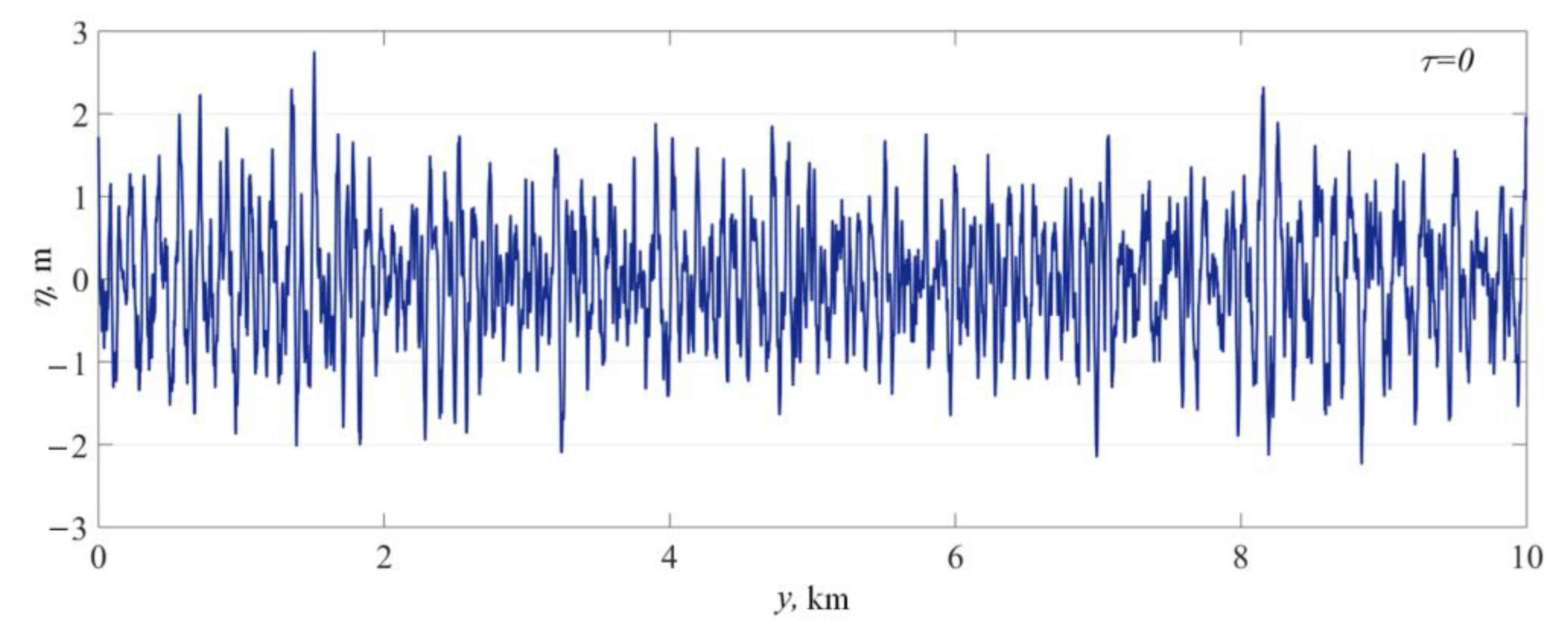
The initial wave field modeled by (4) is shown in Figure 2. The standard deviation is 0.75 m, so the wave with an amplitude equal or bigger than 3 m can be considered to be a freak wave. Here, we use the freak wave c criterion based on the standard deviation of the wave field, because $A_s$ defined as the average of one-third of the highest waves can be different in various moments of time. Thus, using the parameter that is constant in time is more suitable for the calculation of the lifetime of freak waves.

The numerical simulation of Equation (3) with the periodic boundary conditions is based on the pseudo spectral method using several conserved invariants to control the accuracy of the calculations [27]. This method makes it possible to calculate derivatives with respect to a spatial variable in the Fourier space with high accuracy. A finite-difference approach was applied for the time integration.

The chosen solution of Equation (3) describes a complex pattern of superposition of harmonics at different points and times. With a successful combination of circumstances (i.e., the selection of cosine phases), the amplitudes of the harmonics are summed up, which leads to the appearance of waves of large amplitudes at a certain point at a given time (spatiotemporal focusing).

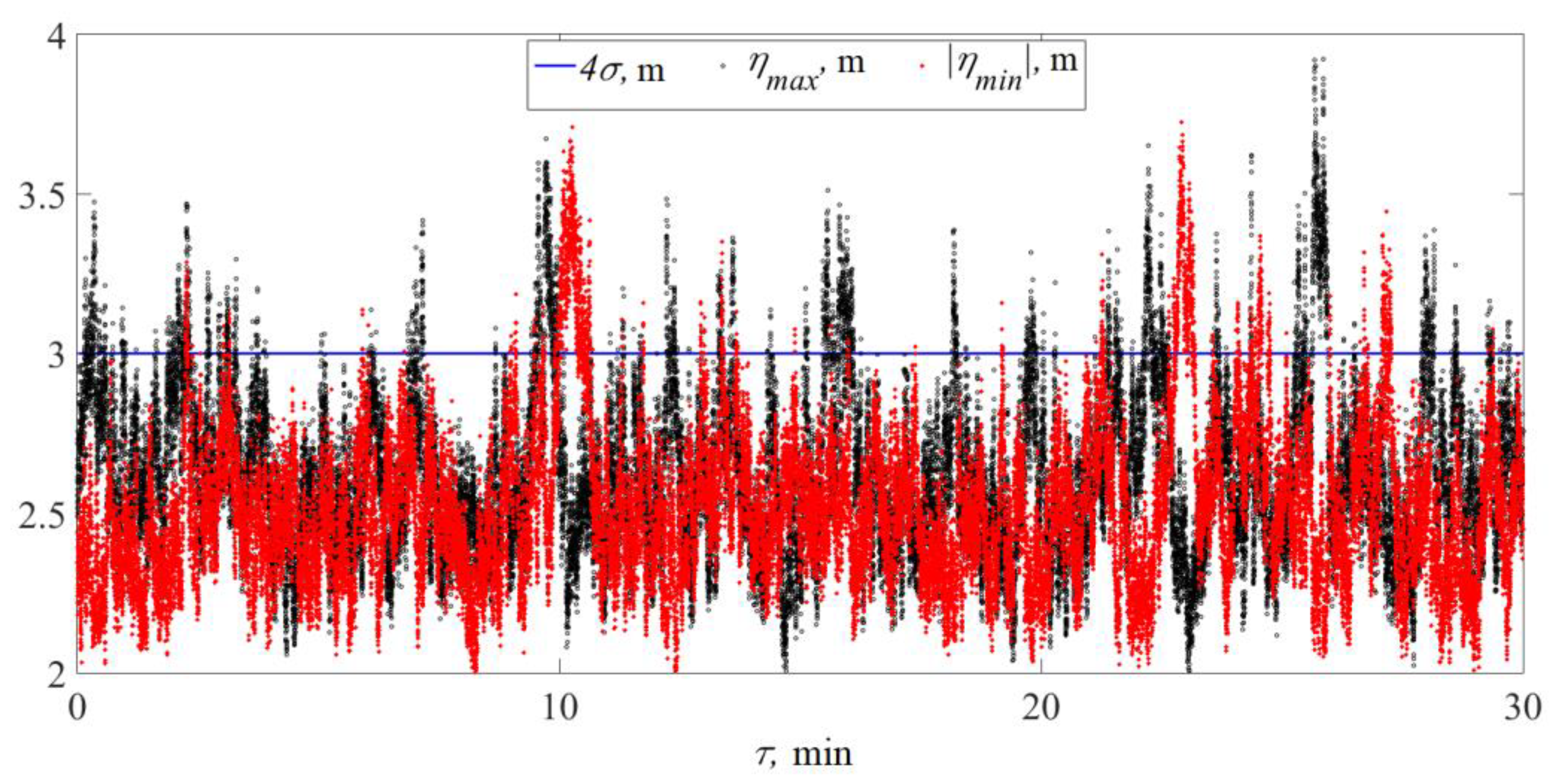
Figure 3, showing the maximum wave field and module of minimum wave field at each time, demonstrates the freak wave appearance in the wave field itself according to the amplitude criterion ($A_s>4\sigma$), both of positive and negative polarity. The maximum positive wave occurred during the time of integration has an amplitude equal to 3.7 m. In this case, the parameter I from Equation (1) equals to 2.46. For negative waves, it is even higher: the maximum negative wave occurred during the time of integration has an amplitude equal to 3.9 m, thus, I = 2.6.

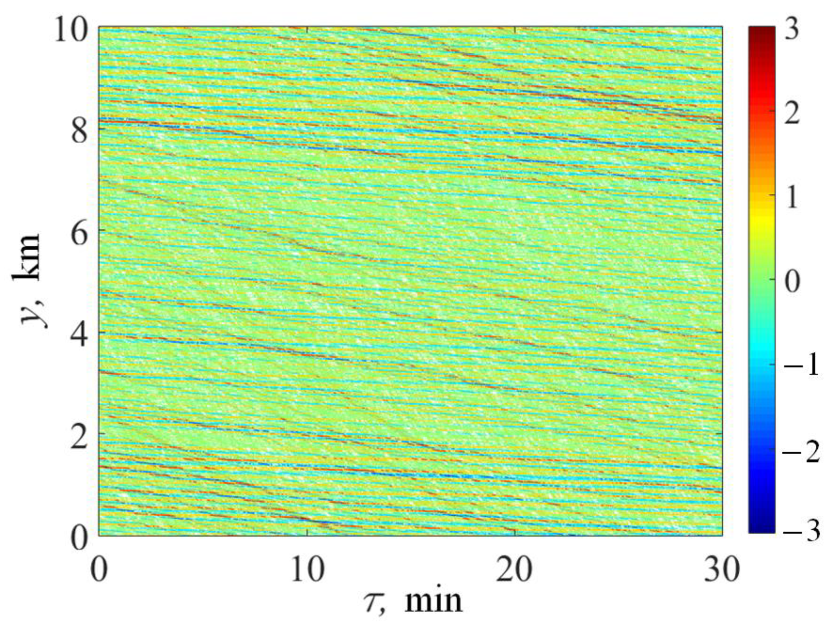
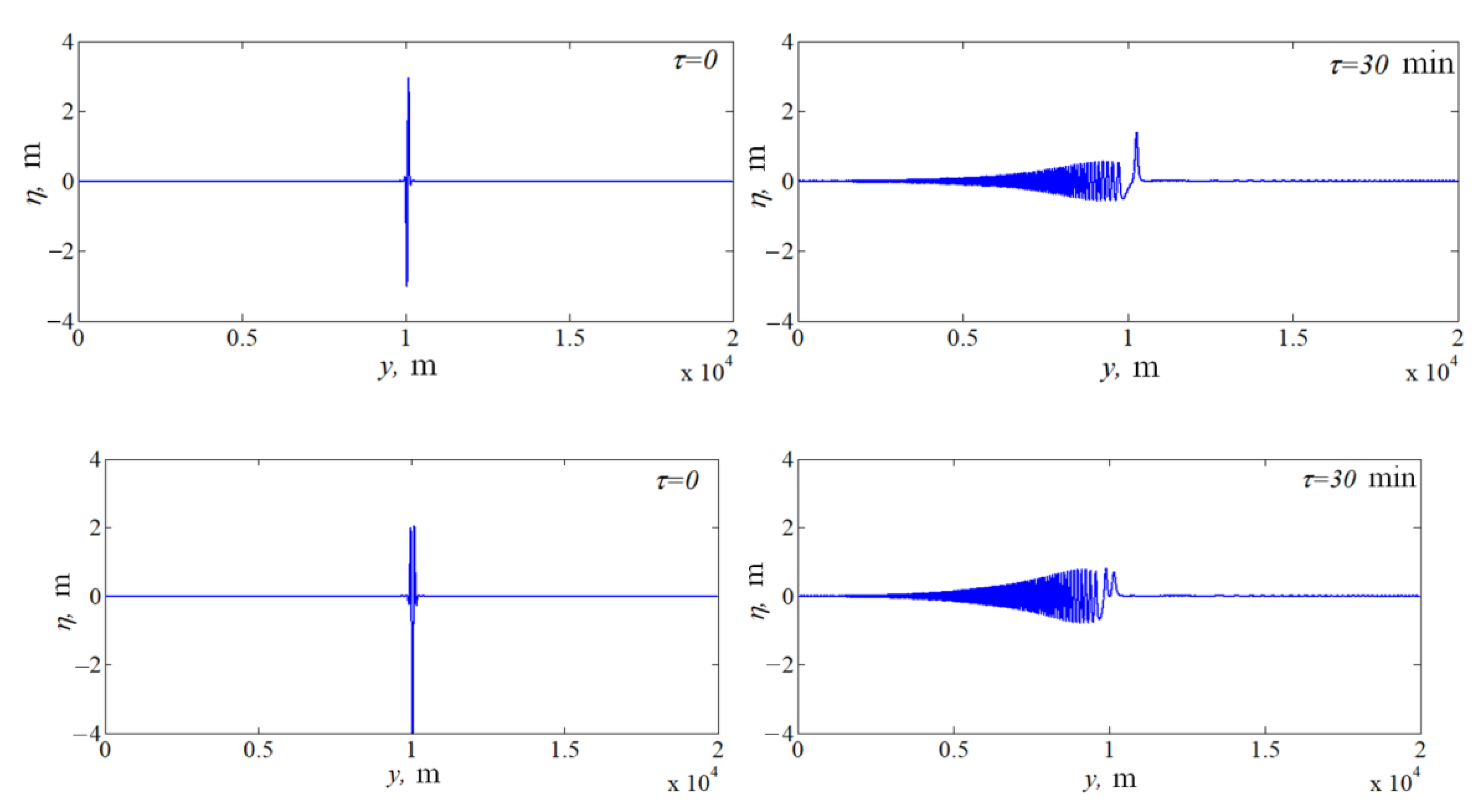
The spatiotemporal diagram of the wind wave field evolution demonstrates the existence of quite intensive wave groups moving with low velocity (Figure 4). They contribute to a short, anomalously large wave formation (Figure 5, clouds of dots on the top and bottom of the figure). However, the lifetime of these freak waves is very short—about several seconds. They are mostly single waves of different polarity. The profiles of positive and negative freak waves are presented in Figure 6.

The evolution of wave spectra is shown in Figure 7 in logarithmic scales. The solid blue curve refers to the initial condition (5), while the red broken curve give the shape of the spectrum at t = 30 min. The evolution of the spectra is essential. It broadens in the low-frequency domain.

3. Freak Wave Evolution against Wind Waves

Above, we considered the evolution of the wave field for the average wave data in this region. In practice, however, there exists a mixture of swell and wind waves (so-called crossing sea). One of the reasons for this in deep water can be the interaction of swell waves coming from the area of a distant storm, with wind waves existing in the area of a local storm [28,29,30]. Typically, statistical methods are used to describe wind waves, while deterministic methods are used to describe swell at large distances from the storm. Since water waves are dispersive, outside the storm zone, the swell is a frequency-modulated packet, and longer waves, which have a higher propagation speed, run ahead of shorter ones. Meanwhile, the wind in the storm zone cannot be considered to be constant, and its variability leads to the generation of wave packets with a very complex law of frequency change with time, including the generation of packets in which short waves run ahead of long ones. Obviously, due to dispersion, such a packet will be focused into an anomalous wave and then spread out over long distances from the storm zone. Thus, at intermediate distances from the storm zone, one can expect the appearance of anomalously large swell waves (freak waves), which also interact with a random field of wind waves associated with a local storm.

The existence of two wave systems is often observed in shallow water [31]. Experimental studies carried out in [32] off the coasts of the United States showed that in 65% of the analyzed data, ocean wave spectra had two or more separated peaks in the frequency domain.

In this section, we analyze the lifetime of freak waves, forming from swell waves, against the wind waves with parameters from the previous section. Due to the unknown swell parameters, but taking into account that swell transforms into a freak wave as a result of dispersive focusing, the swell waves are modeled by wave packets of different shapes at the moment of their maximum amplification, i.e., when they can be considered to be freak waves. Thus, it is assumed that the anomalous swell wave is formed at the initial moment of time. According to the fact that the KdV equation is time-reversal, there is no need to find exact wave forms that will evolve into a freak wave, but consider the propagation of the formed rogue wave and double its lifetime.

In principle, the freak wave can have a different shape, so several possible forms of a freak wave are considered, which are modeled in the following class of modulated waves with a Gaussian envelope:

$${\eta }_1=Aexp\left(-\frac{{\left(y-\varphi \right)}^2}{l^2}\right)\cos \left(k_{0}y\right).$$

(8)

Here, $k_0=0.046{ \mathrm{m}}^{-1}$, as in the previous section, which corresponds to the length of individual wave that is equal to 136 m; $\varphi$ is a wave position in horizontal direction and $l$ is a parameter responsible for the width of the wave packet. By changing $l$, the number of individual waves in the wave packet is changed. Various forms of anomalously large waves, the evolution of which will be considered, are presented in Figure 8. Their heights are 6 m, which corresponds to the metrics of a freak wave for the parameters of the sea state from the previous section.

Within the KdV model, an initial perturbation transforms into a leading wave (soliton) by moving to the right and the wave packet moving to the left [33]. The transformation of wave packets of different shapes is shown in Figure 9. More oscillations in the initial wave packet contribute to the formation of several wave packets after the leading wave.

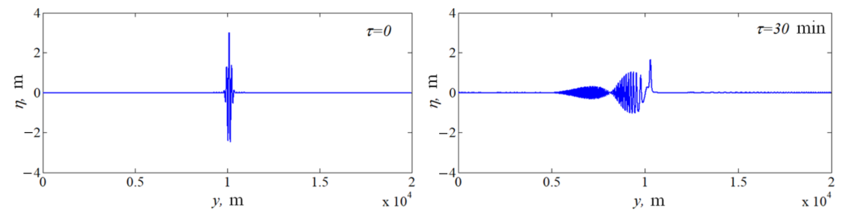
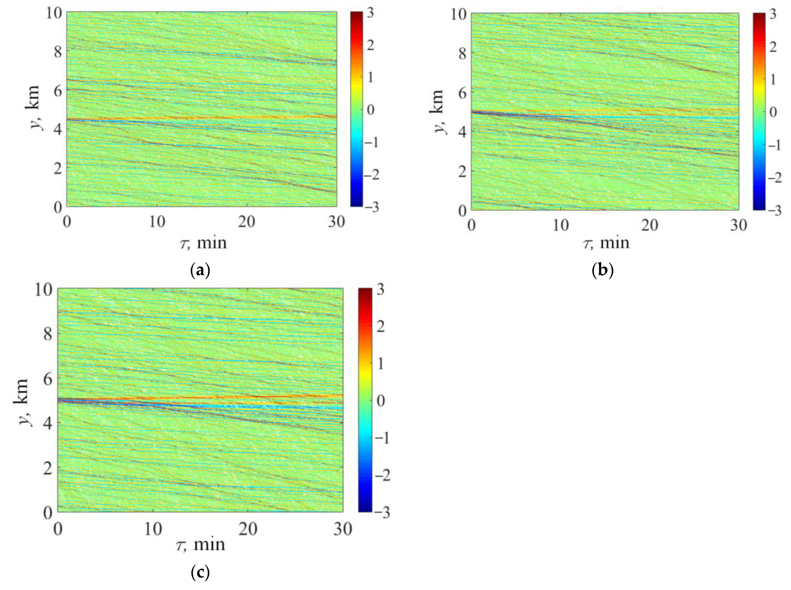
Further, we investigate the dynamics of the wave fields, which is a superposition of a random wave field (4) and a freak wave (8). The evolution of three freak waves of different shapes is shown in Figure 10. At the initial moment of time, the freak waves are clearly observed in the background of wind waves, but after some time, they cannot be detected visually on the oscillograms. However, their traces are well-pronounced in the spatiotemporal diagrams due to their special form with the leading wave moving to the right and dispersive tail moving to the left as well as the larger length, in comparison with wind waves (Figure 11).

The lifetimes of the freak waves have been calculated by cutting the spatiotemporal diagram by levels $\eta >3 \mathrm{m}$ and $\eta <-3 \mathrm{m}$, since $\mathsf{\sigma }$ is equal to 0.75 m, and waves with an amplitude greater than $3$m can be considered freak waves. Figure 12 shows these estimations for freak waves of different shapes. The sign-variable freak wave disappeared very quickly and remains an accidental freak wave in the wind field. Following the length of the small trace of this wave and by multiplying the lifetime by two according to time-reversibility, the lifetime of the sign-variable freak wave can be estimated to be 3–4 min. The symmetry between negative and positive waves can be observed in this case. The time of disappearance of “two sisters” is about 6 min. Further, the short dashes can be observed on the trajectory of the dispersive tail, but they arise for a very short time. Thus, the total lifetime of “two sisters” can be estimated as 12 min. The wave packet called “three sisters” after its formation is visible for 11 min (for positive elevation), after that the wave disappears for quite a long time. For negative elevation, the lifetime is estimated to be about 14 min. Therefore, the total lifetime of this wave packet is about 22–25 min. The trajectories of positive excesses are more pronounced, which is why some asymmetry of the freak wave is present.

These calculations are in good agreement with laboratory experiments with strongly nonlinear waves. In the work [34], the results of a laboratory experiment and numerical simulation of the process of dispersive focusing of a wave packet in the framework of the nonlinear theory are described. In particular, it is shown that the lifetime of a freak wave is 1–3 min. As shown in [23], a linear, single freak wave has about the same lifetime, which is estimated to be 2 min.

4. Conclusions

In this paper, we study the problem of the visibility of anomalous freak waves in the background of moderate wind waves in shallow water. Both wave systems are assumed to propagate in the same direction. For sea surface modeling, the Pierson–Moskowitz spectrum is used. Numerical simulation is performed within the Korteweg–de Vries equation framework. The lifetime of the sign-variable freak wave, “two sisters”, and “three sisters” is analyzed. The lifetime increases with an increasing number of individual waves in the anomalous wave packet. For the ratio $A/A_s=2$ the lifetime of “one, two, and three sisters” is about 4, 12, and 25 min, respectively. It is also shown that random wave field also admits the formation of freak waves but with very short lifetimes (about several seconds).