Composition and Patterns of Taxa Assemblages in the Western Channel Assessed by 18S Sequencing, Microscopy and Flow Cytometry

Abstract

Plankton monitoring by microscopy offers a long-term ecological perspective of plankton communities, but detection approaches are uniquely biased. Genetic identification of marine plankton has become standard but is still not used in routine monitoring. This study assesses the value that genetic methods bring to microscopic and flow cytometry monitoring methods in the Western (English) Channel. An 18S high throughput sequencing (HTS) diversity survey of plankton taxa was performed on samples collected from an automated Water and Microplankton Sampler (WaMS) deployed on the Continuous Plankton Recorder platform (CPR) from 2011–2012. This survey detected contrasting but complementary taxa assemblages to that of microscopic surveys, mostly composed of smaller or naked or thin-walled plankton taxa, with most phytoplankton being under 10 µm infrequently recorded by other surveys. Most genetically-detected taxa in the survey were mixotrophic or heterotrophic. In comparison with microscopic phytoplankton counts from the CPR survey and Western Channel Observatory station L4, only 8–12 taxonomic families were common to all three surveys, most of them dinoflagellates, with a bias towards larger diatoms and dinoflagellate taxa in microscopy surveys. Additional quantitative real-time PCR detection of two potentially harmful taxa, the pelagophyte, Aureococcus anophagefferens and four Pseudo-nitzschia from 2011–2013. This revealed that growth of A. anophagefferens was elevated in the summer of 2011, whilst the appearance of Pseudo-nitzschia delicatissima in February of that year contrasted with it’s timing at a coastal station. Smaller phytoplankton measured by flow cytometry had distinct seasonality and abundance in the mid-Atlantic compared to coastal regions reflecting distinct conditions.

1. Introduction Outline

Phytoplankton sustain marine food webs through the conversion of inorganic CO₂ to biomass, are responsible for approximately 50% of Oceanic primary production [1,2], and are key contributors to oxygen production and nutrient cycling [3]. A key goal in marine phytoplankton ecology is to understand the role of community structure, the drivers that alter their dynamics and the resulting impact on ecosystem dynamics, although how phytoplankton community structure affects nutrient cycling is poorly understood [4]. Monitoring phytoplankton adequately is also essential to meeting the goals of Good Environmental Status, as set out in the Marine Strategy Framework Directive (MSFD) legislature or the UK post-Brexit equivalent, including the maintenance of biodiversity [5]. The Global Ocean Observing System (GOOS) efforts to describe the state of the ocean using Essential Ocean Variables (EOVs) have identified plankton abundance and diversity as one that with moderate to high impact on societal needs [6] whilst the Intergovernmental Science-Policy Platform on Biodiversity and Ecosystem Services (IPBES) has recognized that marine biodiversity has degraded [7].

Currently, only chlorophyll-a (as a proxy for phytoplankton biomass) and microscopic measurements are used in assessments of phytoplankton biodiversity [3]. There is an established baseline of mostly microphytoplankton, typically >20 µm [4], using standardized microscopy methods, including the relative ease in quantifying cells to record diversity, biovolume and biomass estimations. Over the past 20 years, DNA sequencing of marine plankton samples (known as environmental sequencing or eDNA sequencing) has revealed much more extensive diversity than that measured by routine light microscopy. The extensive TARA oceanic survey revealed taxa numbers were 10-fold higher by sequencing than estimated by light microscopy [1], and approximately one-third of eukaryotes could not be identified to any known representative in public genetic databases [8]. Picoplankton (typically from ≤2 µM) and nanoplankton (typically 2–20 µm) [4] are under-represented in routine microscopic phytoplankton surveys due to their size, ambiguous morphology or destruction on preservation [1,8,9]. There has been success in quantifying pico- and nanophytoplankton by flow cytometry (FC), an optical method that can detect cells based on light scattering and photosynthetic pigment fluorescence into different sizes and photosynthetic pigment groups [10]. Taxa resolution is low, with less than 10 identifiable groups from oceanic samples, each representing dozens to thousands of aggregate species groups, but nevertheless produces accurate abundance measurements and additional information on growth rates and cell cycles [10].

The disparity in current routine phytoplankton biodiversity measurements used for official assessments and the actual phytoplankton biodiversity presents knowledge gaps and suboptimal marine management decisions as a result. Genetic-based methods could augment monitoring to cover these gaps. Eukaryotic high-throughput sequencing (HTS) surveys commonly use the 18S ribosomal DNA (rDNA) marker as it is well represented in public databases for comparisons. They are more likely to pick up rare phytoplankton species and picoplankton, although with reduced resolution at the species level [11]. However, there are still hurdles, notably the lack of direct quantification due to bias in amplifying genes combined with the variable copy number of the 18S rDNA marker [12]. Further, there is a dearth of long-term, broad-level comparisons between genetic, microscopic and FC phytoplankton monitoring methods. There is a need to assess and generate baseline level comparisons in line with official timelines, at least seven years for OSPAR [13]

The Western English Channel (hereafter called the Western Channel), part of the Celtic Sea, is a well-studied marine system characterized by Atlantic influence with riverine influences and summer thermal stratification influenced by offshore stratification and turbidity influenced by wave height [14]. Pico- and nanophytoplankton account for 48% of primary productivity, and changes in phytoplankton species assemblages directly influence primary productivity in this region, underpinning the importance of measuring diversity [15,16]. Several overlapping long-term phytoplankton surveys monitor this region, including the Continuous Plankton Recorder (CPR) PR-route transect from Roscoff to Plymouth since 1975 [17] and the Western Channel Observatory single monitoring station L4 (WCO-L4), located nearby, since 1992 along with physicochemical parameters [18]. From 2011–2016, small-volume (≤200 mL) samples collected were collected using the automated Water and Microplankton Sampler (WaMS) within the payload of the CPR device and alongside the CPR survey to capture smaller phytoplankton alongside the larger phyto- and zooplankton captured by the CPR platform [17]. The WaMS machine and its preliminary biodiversity data generated by high-throughput sequencing (HTS) have been reported [19] but only for four months between February–May 2011, where the WaMS biodiversity in the smaller, soft-shelled or flagellated plankton. In this study, we extend HTS-generated biodiversity assessment over 1 year (2011–2012) to capture all seasons where phytoplankton growth and diversity are at their peak and compare this to those generated by microscopy from equivalent CPR survey transects and the WCO-L4.

We selected the harmful algal diatom genus, Pseudo-nitzschia (cleve) H. Peragallo, on their potentially harmful nature but lack of species- resolution in this region. Their presence is recorded in the Western Channel by the WCO and CPR survey and to genus level by earlier WaMS validation study [19,20,21]. Of the 52 species, approximately half produce the toxin domoic acid causing Amnesiac Shellfish Poisoning in humans and marine animals [22]. These can only be distinguished into two to six morphospecies groups using light microscopy due to their small or delicate ultrastructural features [23]. Three morphospecies groups have previously been identified at WCO-L4: the Pseudo-nitzschia delicatissima group, the Pseudo-nitzschia seriata group and the Pseudo-nitzschia pungens/multiseries sometimes to high levels with domoic acid associated with the latter two groups [24]. Whilst toxin production is found to be endogenous for at least one species [25], there are numerous exogenous triggers, including temperature, salinity, phosphate, nitrate, silicate, macronutrients and in other regions, iron and ocean acidification [24,26,27] that hinder our understanding of environment cues governing growth and toxin production. Validated qRT-PCR assays Pseudo-nitzschia species [28] were used here together with an additional in-house assay to confirm the presence of potentially toxic Pseudo-nitzschia fraudulenta and P. multiseries and likely non-toxic P. delicatissima species. Further, to assess if genetically-detected Pseudo-nitzschia species growth is similar to that of their corresponding morphospecies group and to assess likely physiochemical growth stimuli: nutrients or Sea surface temperature (SST).

The second harmful algae species evaluated here is the 2 µm pelagophyte Aureococcus anophagefferens using a validated qRT-PCR method [29]. This species is recorded to grow to high densities on the east coast of the USA and South Africa, known as brown tide events, killing marine life, including commercial shellfish, through deoxygenation, poor light and toxins [30]. It has been found in ballast water with an increasing geographical distribution in the USA and other parts of the world [31] and is, therefore, likely to be cosmopolitan with the potential for nuisance growth under the right conditions. A. anophagefferens has previously been detected in the Western Channel [19] in our validation study of WaMS, and, as picoplankton are more abundant, is likely to be in sufficient abundance in small-volume WaMS water samples. Here we track its seasonal trends and compare it to similarly sized picophytoplankton groups measured by FC.

This study has three objectives to understand how genetically acquired species data can contribute towards routine monitoring methods to improve marine assessment. (1) To assess the capacity of a small-volume WaMS sampling system to capture harmful algae as measured by qRT-PCR route transect. (2) To compare single-species seasonal abundance of WaMS with phytoplankton communities from WaMS FC phytoplankton and WCO L4 and CPR surveys over the 2011–2013 period to determine the level of correspondence and additional spatio-temporal information they bring. (3) What phytoplankton assemblages are detected by standard HTS methods, FC and microscopy, and how much do they overlap or extend the taxonomic assemblages detected? Finally, we discuss the relative strengths of each method and propose measures of improvement to develop complete phytoplankton monitoring.

2. Materials and Methods

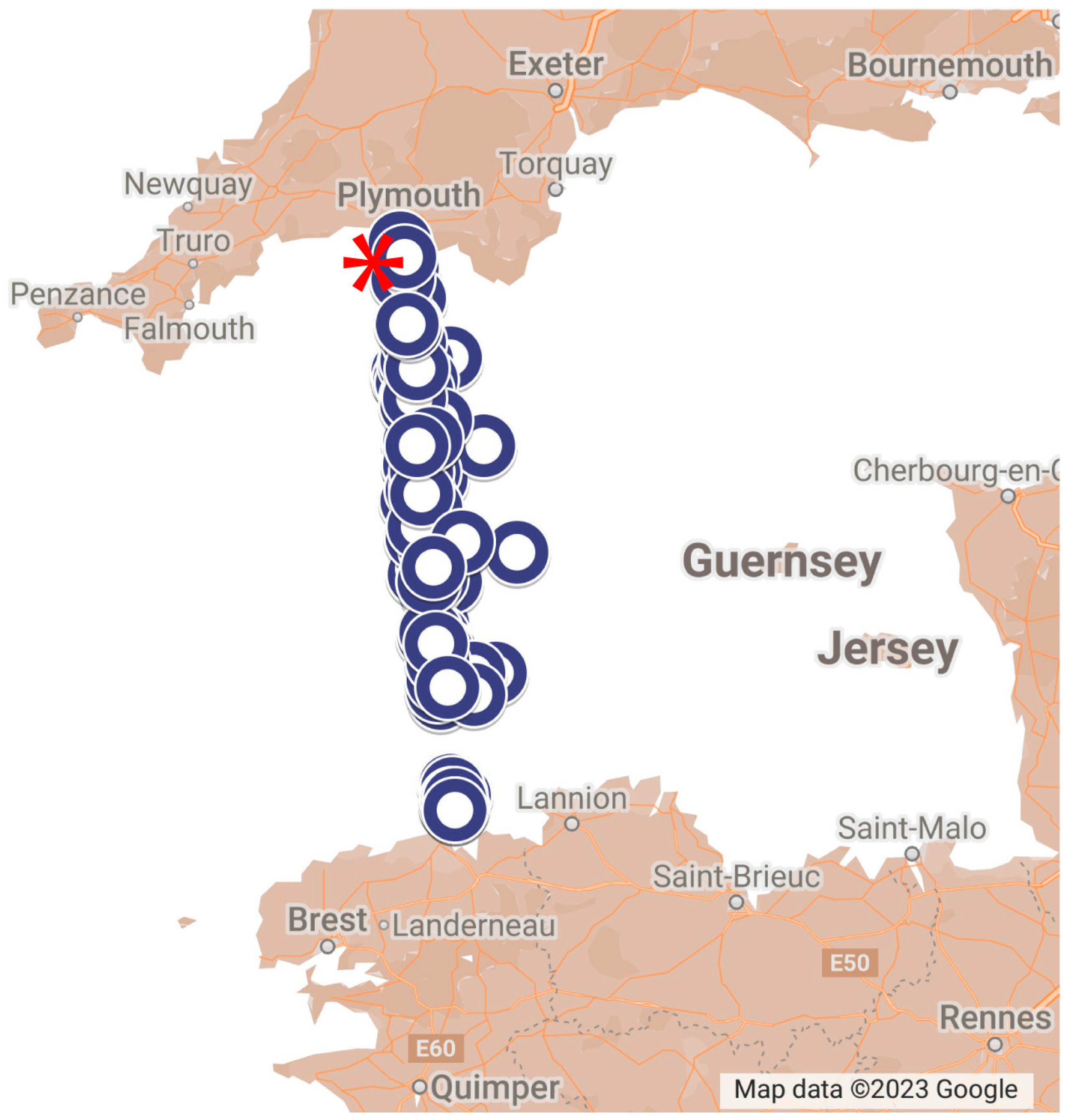
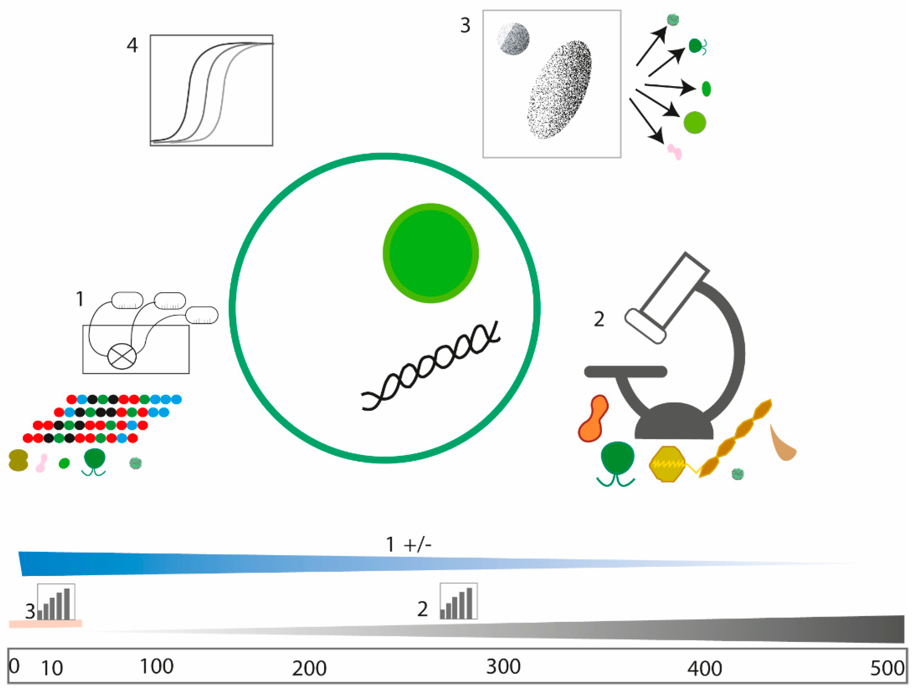
2.1. Sampling Phytoplankton in the Western Channel by WaMS, WCO L4 and CPR Survey

The Water and Microplankton Sampler (WaMS) mechanism and sample collection are described elsewhere [19]. Approximately monthly sampling was deployed within the payload of a Continuous Plankton Recorder (CPR) instrument on a Ship of Opportunity operated by Brittany Ferries from 2011 to 2013 over a transect of the Western Channel between Roscoff, France and Plymouth, UK (see Figure 1) from latitude and longitude of approximately 48.03, −3.93–50.01, −4.13. Briefly, the WaMS pumps 200–500 mL of water directly into 10 sampling bag pre-programmed sampling stations along a 122-mile transect and is processed immediately after collection. Seawater from two bags per station) were pooled, filtered onto a 0.2-µm membrane filter and preserved in ethanol at −80 °C until DNA extraction as described in Section 2.4. All samples are listed in Table S1. Sampling interruptions occurred in January, August and November 2011 and in January and April 2012. In March–April 2013, the machine went into repairs and was not available for sampling, and in December 2013, WaMS sampling could not be scheduled.

Phytoplankton from Western Channel Observatory’s Station L4 (WCO_L4) monitoring site (50 15.0′ N; 4 13.0′ W), situated off the south-west coast of England, United Kingdom, on a weekly basis (weather permitting) at 10 m depth since October 1992. This is the nearest WaMS station 5. Paired 200 mL water samples were collected using a 10 L Niskin bottle attached to a CTD and were fixed in acid Lugol’s iodine [32] for enumerating all phytoplankton cells >2 μm and neutral formaldehyde for enumerating coccolithophores. Silicate, Phosphate, Nitrite, Nitrate and Ammonia nutrients and SST were measured from seawater collected from WCO L4 on a weekly basis from a CTD/rosette system at various depths as described in File S1, according to protocols and standards in [33]. From 2000–2006 nutrient measurements were taken from frozen samples, so they may be altered, especially ammonia measurements. The SST and nutrients 20 and 21-year respective baselines of data were used as a comparison for the study period 2011–2013. The final nutrient dataset from 2000–2020 is available at doi:10.5285/d61b955c-93b2-681f-e053-6c86abc0378e, accessed on 19 December 2022 and a summary of average values is presented in supplementary Table S12. The SST dataset from 2000–2020 is found in Table S13.

Plankton sampling using the CPR survey collection is described in detail elsewhere [17,34]. This study used samples collected on a Ship of Opportunity operated by Brittany Ferries from 2011 to 2012 in the Western Channel between Roscoff, France and Plymouth from 2011 to 2012 (see Figure 1).

2.2. Extraction of Microscopic Phytoplankton Datasets from the Western Channel

To compare the diversity of phytoplankton obtained from WaMS with that of other microscopic datasets collected from the same platform or nearby Phytoplankton species and cell counts were obtained from the Western Channel Observatory’s Station L4 (WCO_L4) weekly phytoplankton time-series from 2011–2013 [35] containing taxa-specific and total functional group abundance (cells mL⁻¹) and biomass (mgC m⁻³) data. The abundance of each taxon (cells mL⁻¹) was calculated according to the number of individuals per unit volume of the sub-sample analyzed. Samples are taxonomically classified and counted at Plymouth Marine Laboratory according to the Utermöhl counting technique [36], and since 2016, these methods follow the British and European standard document “Water quality—Guidance standard for routine microscopic surveys of phytoplankton using inverted microscopy (Utermöhl technique)” (BS EN 15204:2006).

Phytoplankton from the CPR survey counting is quality assured and recorded in a semi-quantitative manner using log-transformed data [17]. The dataset used is available at DOI: https://doi.org/10.17031/1808, accessed on 29 December 2021. Before the presence or absence analysis of phytoplankton taxa to compare with those found in other phytoplankton datasets here, Vorticella sp. and nematocysts were excluded as non-phytoplankton entities, whilst Brown cysts, Black Spine cyst, Filamentous algae and phytoplankton color were excluded as too ambiguous. Additionally, Pseudo-nitzschia delicatissima complex and Pseudo-nitzschia seriata complex cell counts were extracted from this dataset. All sample log-transformed counts were averaged per month for each taxon to remove spatial components and for ease of comparison with the monthly averaged WaMS Pseudo-nitzschia qRT-PCR dataset. These were plotted to compare seasonality with WCO L4, and the WaMS Pseudo-nitzschia dataset was towed alongside the CPR survey.

2.3. Enumeration of Phytoplankton and Bacteria by Flow Cytometry (FC)

Duplicate 2 mL WaMS samples were preserved for flow cytometry in 1% TEM-grade Gluteraldehyde (Sigma) flash-frozen and stored at −80 °C for 24 h before thawing for flow cytometry detection. The following photosynthetic plankton groups, Synechococcus, Prochlorococcus, Cryptophytes, Coccolithophores, Picoeukaryotes and Nanoeukaryotes, were enumerated as described by [19]. The complete flow cytometry dataset from 2011–2016 from which this data was extracted is available at DOI https://doi.mba.ac.uk/data/2955, accessed on 16 November 2022. Only the cyanobacteria Synechococcus spp. and picoeukaryote and nanoeukaryote data were used for further analysis, the former 2 being of similar size and the latter overlapping in size and their potential predators. To increase robustness, data from all positions from each cruise were aggregated into mean values. Flow cytometry data from WCO L4 was provided by G.T (pers. Comm) and available at doi:10.5285/908f84ec-d20c-7c88-e053-6c86abc08fda, accessed on 17 February 2023.

2.4. WaMS Sample DNA Extraction for Diversity Assessment and Quantitative Assessments of Potential Harmful Algae

For WaMS samples from February to March 2011, DNA extraction was performed as described in [19]. All other samples were extracted by CTAB buffer extraction, followed by a phenol-chloroform extraction process adapted from [37] as described by 500 µL of CTAB buffer containing 5.6 µg/mL of Proteinase K and 0.2% ß-Mercaptoethanol (Sigma) was added to each sample and incubated for 1 h 30 min at 55 °C. DNA was extracted using equal volumes of phenol (Sigma), followed by a chloroform/isoamylalcohol mix (Sigma). DNA was precipitated with isopropanol and washed twice with ice-cold 70% ethanol. The pellet was resuspended in 60 µL of TE buffer.

2.5. Quantitative Real-Time PCR-HRM Assays of Potentially Harmful Algae Species of WaMS Samples

All quantitative assays were assessed through High-Resolution Melt-Curve (HRM) quantitative real-time PCR (qRT-PCR) that melts the PCR product at a specific temperature for species detection and simultaneously carries out qRT-PCR on DNA in a Rotor-Gene 6000 (Qiagen, Valencia, FL, USA). Cultures of known algae species were grown to extract DNA and generate PCR products that acted as quantitative standards in a dilution series for HRM-qRT-PCR assays. Genomic DNA from these cultures also acted as positive controls. DNA, extraction, preparation of standards and assay conditions are described in File S2.

Table 1. qRT-PCR assays developed, species, primers, years tested.

Assay	Reference	Marker	Primers	Size of Product/bp	Standard Range Copies/µL
Pseudo-nitzschia fraudulenta	Andre et al. (2011) [28]: PN5. 8SF-HRM, QPfrauR-HRM	ITS1	PN5.8SF-HRM 5′ CAGCGGTGGATGTCTAGGTTC−3′ QPfrauR-HRM 5′ CCGCTGCTAGAGCGGTCAGAG 3′	225	3.18 × 108–3.17 × 106
Pseudo-nitzschia multiseries	PMulsF (this study), PN5. 8SR-HRM (Andre et al., 2011) [28]	ITS2	PMulsF-HRM 5′ CTAGACTACTGTAGTCAAACTTAACCGGCAAC 3′ PN5.8SR-HRM 5′ GAACCTAGACATCCACCGCTG 3′	201	5.75 × 108–5.75 × 104
Pseudo-nitzschia delicatissima	QPdelRa2F (this study), PN5. 8SR-HRM (Andre et al., 2011) [28]	ITS	QPdelRa2F GTGCAATACTTTGTTGGGTTTCG PN5.8SR-HRM 5′ GAACCTAGACATCCACCGCTG 3′	182	2.5 × 102 to 2.5 × 107
Aureococcus anophagefferens	Aa1685f, Popels et al., 2003, [29] Euk B (Medlin et al., 1988) [39]	18S	Aa1685f ACCTCCGGACTGGGGTT, EukB	118	102–106

summarizes the assay species and gene marker targets, the primers used and the detectable cell range. Based on previous occurrences in WCO-L4, Pseudo-nitzschia fraudulenta and Pseudo-nitzschia delicatissima were chosen based on a previously validated study [28]. A potentially toxic Pseudo-nitzschia multiseries assay was developed [38] because of its possible presence reported by [24]. Aureococcus anophagefferens was chosen because of its previous detection in WaMS [19] using an assay developed in [29].

Melt curves from standards, positive and negative controls and environmental samples were inspected to assess contamination and peak temperature and range of curves. HRM standard reports were downloaded from the Corbett Rotor-Gene 6000 software (Qiagen), shown in Figure S1 of File S2. A selection of environmental samples and positive control PCR products were checked through DNA sequencing (Source Bioscience (Nottingham, UK) using their guidelines to confirm specific species detection (see Results Section 3.2).

To quantify species from WaMS samples, DNA copy numbers were converted to cell concentrations using known DNA copy numbers as standards as described in File S2. The qRT-PCR run parameters for P. fraudulenta and P. multiseries (File S2, Table S1) showed low reaction efficiency, so these species were excluded from subsequent quantification assessments, and only their presence was recorded (

Table 2. Summary of Samples taken in the English Channel from 2011–2013 using the WaMS deployed within the CPR sampling platform and tests carried out on them. All CPR tow samples will have microscopic plankton semi-quantitative abundance. Empty positions indicate no samples were available to analyze. No samples were taken in August and November 2011, April 2012, March, April and October 2013. Positions E1–E5 denote sample positions taken progressively from Roscoff, France to Plymouth, UK. Blue-type sample positions were not collected, so they were inferred from the timing of previous deployments. Pn: Position, Y: Year, M: month, Lat: Latitude, Lon: Longitude, In situ T: In situ temperature, FC: Flow cytometry. AA: A. anophagefferens, PD: P. delicatissima, PF P. fraudulenta, PM: P. multiseries.

									HRM-qRT-PCR Test
CPR Tow	Pn	Y	M	Lat	Lon	T.	FC	Seq Sample	AA	PD	PF	PM
344PR	E1	2011	2	48.03	−3.83	9.56	Yes	WS1	Yes	Yes	Yes
		2011	2
		2011	2
		2011	2
	E5	2011	2	49.94	−4.12	9.31	Yes	WS2	Yes	Yes	Yes
345PR		2011	3
	E2	2011	3	49.28	−4.02	9.75	Yes	WS3	Yes	Yes	Yes
		2011	3
		2011	3
	E5	2011	3	49.78	−4.12	9.78	Yes	WS4	Yes	Yes	Yes
346PR	E1	2011	4	48.80	−3.96	10.5	Yes	WS5	Yes	Yes	Yes
	E2	2011	4	49.08	−4.01	10.25	Yes	WS6	Yes	Yes	Yes
	E3	2011	4	49.37	−4.04	10.08	Yes	WS7	Yes	Yes	Yes
	E4	2011	4	49.67	−4.11	10.17	Yes	WS8	Yes	Yes	Yes
	E5	2011	4	49.97	−4.17	10.18	Yes	WS9	Yes	Yes	Yes
347PR	E1	2011	5	48.82	−3.93	N/A	Yes	N/A	Yes	Yes	Yes
	E2	2011	5	49.11	−3.98	11.95	Yes	WS10	Yes	Yes	Yes
	E3	2011	5	49.40	−3.97	12.4	Yes	WS11	Yes	Yes	Yes
	E4	2011	5	49.68	−4.03	12.56	Yes	WS12	Yes	Yes	Yes
	E5	2011	5	49.95	−4.09	12.38	Yes	WS13	Yes	Yes	Yes
348PR	E1	2011	6	48.78	−3.96	13.7	yes	WS14	Yes	Yes	Yes
	E2	2011	6	49.10	−4.02	12.9	yes	WS15	Yes	Yes	Yes
	E3	2011	6	49.42	−4.10	13.9	yes	WS16	Yes	Yes	Yes
	E4	2011	6	49.68	−4.10	13.9	yes	WS17	Yes	Yes	Yes
	E5	2011	6	49.96	−4.13	13.9	yes	WS18	Yes	Yes	Yes
349PR	E1	2011	7	48.83	−3.96	14.5	yes	WS19	Yes	Yes	Yes
	E2	2011	7	49.16	−4.02	14.4	yes	WS20	Yes	Yes	Yes
	E3	2011	7	49.41	−4.04	15.3	yes	WS21	Yes	Yes	Yes
	E4	2011	7	49.70	−4.09	15.7	yes	WS22	Yes	Yes	Yes
	E5	2011	7	49.97	−4.13	15.7	yes	WS23	Yes	Yes	Yes
351PR	E1	2011	9	48.81	−3.93	N/A	yes	WS24	Yes	Yes	Yes
	E2	2011	9	49.15	−3.78	N/A	yes	WS25	Yes	Yes	Yes
	E3	2011	9	49.48	−3.69	N/A	yes	WS26	Yes	Yes	Yes
	E4	2011	9	49.77	−3.83	N/A	yes	WS27	Yes	Yes	Yes
	E5	2011	9	50.01	−3.97	N/A	yes	WS28	Yes	Yes	Yes
352PR	E1	2011	10	48.81	−3.95	14.7	yes	WS29	Yes	Yes	Yes
	E2	2011	10	49.13	−4.00	14.9	yes	WS30	Yes	Yes	Yes
	E3	2011	10	49.39	−4.05	15.0	yes	WS31	Yes	Yes	Yes
	E4	2011	10	49.79	−4.08	14.9	yes	WS32	Yes	Yes	Yes
	E5	2011	10	49.93	−4.10	14.7	yes	WS33	Yes	Yes	Yes
354PR	E1	2011	12	48.79	−3.96	13.0	yes	WS34	Yes	Yes	Yes
	E2	2011	12	49.15	−4.01	12.7	yes	WS35	Yes	Yes	Yes
	E3	2011	12	49.41	−4.03	12.5	yes	WS36	Yes	Yes	Yes
	E4	2011	12	49.70	−4.06	12.3	yes	WS37	Yes	Yes	Yes
	E5	2011	12	50.00	−4.09	12.0	yes	WS38	Yes	Yes	Yes
355PR	E1	2012	2	48.31	−3.95	10.3	yes	WS39	Yes	Yes	Yes
	E2	2012	2	49.12	−4	10.6	yes	WS40	Yes	Yes	Yes
	E3	2012	2	49.44	−4.06	10.3	yes	WS41	Yes	Yes	Yes
	E4	2012	2	49.72	−4.12	10.2	yes	WS42	Yes	Yes	Yes
	E5	2012	2	49.95	−4.16	9.7	yes	WS43	Yes	Yes	Yes
356PR	E1	2012	3	48.82	−3.96	10.40	yes		Yes	Yes
	E2	2012	3	49.15	−3.98	10.70	yes		Yes	Yes
	E3	2012	3	49.44	−4.06	10.10	yes		Yes	Yes
	E4	2012	3	49.72	−4.12	10.30	yes		Yes	Yes
	E5	2012	3	49.95	−4.16	10.10	yes		Yes	Yes
358PR	E1	2012	5	48.81	−3.96	11.9	yes		Yes	Yes
	E2	2012	5	49.25	−4.02	11.6	yes		Yes	Yes
	E3	2012	5	49.61	−4.06	11.6	yes		Yes	Yes
	E4	2012	5	49.95	−4.07	12.2	yes		Yes	Yes
	E5	2012	5	50.27	−4.17	11.4	yes		Yes	Yes
359PR	E1	2012	6	48.80	−3.96	13.41	yes		Yes	Yes
	E2	2012	6	49.20	−4.02	13.22	yes		Yes	Yes
	E3	2012	6	49.62	−4.13	13.6	yes		Yes	Yes
	E4	2012	6	49.94	−4.15	13.8	yes		Yes	Yes
	E5	2012	6	50.25	−4.16	14.2	yes		Yes	Yes
360PR	E1	2012	7	48.80	−3.96	14.65	yes		Yes	Yes
	E2	2012	7	49.25	−4.06	14.90	yes		Yes	Yes
	E3	2012	7	49.65	−4.11	15.05	yes		Yes	Yes
	E4	2012	7	49.99	−4.14	14.87	yes		Yes	Yes
		2012	7
361PR	E1	2012	8	48.80	−3.96		yes		Yes	Yes
	E2	2012	8	49.26	−4.05		yes		Yes	Yes
	E3	2012	8	49.66	−4.09		yes		Yes	Yes
	E4	2012	8	50.00	−4.13		yes		Yes	Yes
	E5	2012	8	50.32	−4.18		yes		Yes	Yes
362PR		2012	9	48.8	−3.96		Yes
		2012	9	49.26	−4.05		Yes
		2012	9	49.66	−4.09		Yes
		2012	9	50.00	−4.13		Yes
		2012	9	50.33	−4.18		Yes
364PR	E1	2012	10	48.84	−3.97	14.40	yes		Yes	Yes
	E2	2012	10	49.21	−3.99	14.5	yes		Yes	Yes
	E3	2012	10	49.55	−4.02	14.5	yes		Yes	Yes
	E4	2012	10	49.9	−4.13	14.3	yes		Yes	Yes
	E5	2012	10	50.25	−4.15	14.5	yes		Yes	Yes
Additional	E1	2012	10	48.84	−3.97	14.40	yes		Yes	Yes
	E2	2012	10	49.21	−3.99	14.5	yes		Yes	Yes
	E3	2012	10	49.55	−4.02	14.5	yes		Yes	Yes
	E4	2012	10	49.9	−4.13	14.3	yes		Yes	Yes
	E5	2012	10	50.25	−4.15	14.5	yes		Yes	Yes
365PR	E1	2012	11	48.83	−3.96	13	yes		Yes	Yes
	E2	2012	11	49.22	−4.01	13.5	yes		Yes	Yes
	E3	2012	11	49.6	−4.05	13.6	yes		Yes	Yes
	E4	2012	11	49.92	−4.09	13.2	yes		Yes	Yes
		2012	11				yes
366PR	E1	2012	12	48.8	−3.96	11.3	yes		Yes	Yes
	E2	2012	12	49.19	−4.01	12	yes		Yes	Yes
	E3	2012	12	49.52	−4.11	11.8	yes		Yes	Yes
	E4	2012	12	49.88	−4.13	11.6	yes		Yes	Yes
	E5	2012	12				yes
367PR	E1	2013	1	48.78	−3.96		yes		Yes	Yes
	E2	2013	1	49.15	−4.02		yes		Yes	Yes
	E3	2013	1	49.49	−4.05		yes		Yes	Yes
	E4	2013	1	49.84	−4.01		yes		Yes	Yes
	E5	2013	1	50.17	−4.12		yes		Yes	Yes
368PR	E1	2013	2	48.8	−3.96		yes		Yes	Yes
	E2	2013	2	49.13	−4.02		yes		Yes	Yes
	E3	2013	2	49.4	−4.06		yes		Yes	Yes
	E4	2013	2	49.7	−4.09		yes		Yes	Yes
	E5	2013	2	50.05	−4.12		yes		Yes	Yes
371PR		2013	5	48.78	−3.94
		2013	5	49.15	−3.87
		2013	5	49.51	−3.92
	E4	2013	5	49.79	−4.05				Yes	Yes
	E5	2013	5	50.1	−4.14				Yes	Yes
372PR	E1	2013	6	48.78	−3.94				Yes	Yes
	E2	2013	6	49.15	−3.87				Yes	Yes
	E3	2013	6	49.51	−3.92				Yes	Yes
	E4	2013	6	49.79	−4.05				Yes	Yes
	E5	2013	6	50.1	−4.14				Yes	Yes
374PR	E1	2013	7	48.80	−3.95		yes		Yes	Yes
	E2	2013	7	49.18	−4.02		yes		Yes	Yes
	E3	2013	7	49.55	−4.10		yes		Yes	Yes
	E4	2013	7	49.90	−4.12		yes		Yes	Yes
	E5	2013	7	50.22	−4.17		yes		Yes	Yes
375PR	E1	2013	8	48.77	−3.95		yes		Yes	Yes
	E2	2013	8	49.23	−4.03		yes		Yes	Yes
	E3	2013	8	49.64	−4.09		yes		Yes	Yes
	E4	2013	8	49.98	−4.11		yes		Yes	Yes
	E5	2013	8	50.28	−4.16		yes		Yes	Yes
376PR	E1	2013	9						Yes	Yes
	E2	2013	9	49.09	−3.87		yes		Yes	Yes
	E3	2013	9	49.51	−3.92		yes		Yes	Yes
	E4	2013	9	49.79	−4.05		yes		Yes	Yes
	E5	2013	9	50.09	−4.14		yes		Yes	Yes
	E6	2013	9
	E7	2013	9
	E8	2013	9
	E9	2013	9
	E10	2013	9
378PR	E1	2013	11	48.78	−3.95		yes		Yes	Yes
	E2	2013	11	49.12	−3.98		yes		Yes	Yes
	E3	2013	11	49.45	−4.04		yes		Yes	Yes
	E4	2013	11	49.78	−4.11		yes		Yes	Yes
	E5	2013	11	50.11	−4.15		yes		Yes	Yes

). P. delicatissima and A. anophageffrens assays were assessed for quality assurance by a reaction efficiency threshold of 90% (see

Table 3. Reaction efficiency of qRT-PCR assays in this study PD (P. delicatissima), AA (Aureoccocus anophagefferens) for assay run 2011, 2012 and 2013. E = efficiency, M = slope, B = offset or y-intercept, R, R² values indicate fit to the equation.

	PD 2011	PD 2012	PD 2013	AA 2011	AA 2012	AA 2013 pt1	AA 2013 pt2
R	0.999	0.999	0.996	0.994	0.994	0.998	0.984
R2	0.985	0.997	0.992	0.987	0.9888	0.995	0.969
M	−3.935	−2.900	−3.266	−3.502	−3.858	−3.979	−3.223
B	36.361	28.489	34.76	43.483	43.900	38.268	29.398
E	0.872	1.212	1.023	0.9302	0.8163	0.7837	0.6076

) and inter-variability of standard Ct values between qRT-PCR runs (see File S2). The latter was carried out using a 2-tailed student’s t-test with unequal variances.

A total of 98 separate WaMS samples were screened in 2011 (33), 2012 (34) and 2013 (31) for P. delicatissima, 95 for A. anophagefferens assay (37 for 2011, 33 for 2012 and 24 for 2013), whilst 77 were used for P. fraudulenta and P. multiseries assays to cover 2011–2012 period. No replicates were performed for WaMS DNA samples. To improve the temporal coverage of seasonal variation, an average was taken of all samples at each sampling month to account for sampling gaps. Calculated cell concentrations are shown in supplementary Tables S8 and S9 for P. delicatissima and A. anophagefferens, respectively. Average cell concentrations of A. anophagefferens are additionally shown in Table S9b.

2.6. DNA Amplification, High Throughput Sequencing (HTS) and Bioinformatic Analysis of WaMS DNA Samples from 2011–2012

PCR amplification of a 500 bp portion of the variable V4 region of the nuclear 18S rRNA marker was performed on 43 samples of genomic DNA. These were shipped in two batches (WS1-13 then WS13-43) to Molecular Research LP (http://www.mrdnalab.com, accessed on 20 December 2022, Shallowater, TX, USA). A second round of amplification was performed on each batch separately using adaptor-linked barcoded eukaryotic primer pair euk516F (5′-GGAGGGCAAGTCTGGT−3′) and euk1055R (5′-CGGCCATGCACCACC−3′) and HotStarTaq Plus Master Mix Kit (QIAGEN) under the following conditions: initial denaturation at 94 °C for 3 min, followed by 30 cycles of 94 °C for 30 s, 53 °C for 40 s and 72 °C for 1 min, concluding with an elongation step at 72 °C for 5 min. Amplicons were pooled in equimolar concentrations and purified using Agencourt AMPure beads (Agencourt Bioscience, MA, USA). Amplicon libraries were pyrosequenced using Roche 454 GS-FLX Titanium chemistry (hereafter called HTS for high throughput sequencing).

Raw unidirectional sequence data were processed using QIIME v1.9.1 [40]. In the first round of screening, the sequence reads were checked for the presence of the forward sequencing primer (euk516F), and a valid barcode and single reads were removed (the denoising step). This process was carried out separately for reads from February to May 2011 (WS1-13) and from May 2011 to February 2012 (WS14-43). The output files for both of these were combined, and 43 samples in total were processed. Barcoded reads were imported and had forward primers removed (allowing for a maximum of one mismatch) before being demultiplexed and filtered according to their Phred quality scores. Quality criteria were a minimum read length of 200 bp, a maximum read length of 700 bp, no ambiguous bases and a maximum homopolymer length of 6 (as homopolymer reads are a specific problem to 454 GS-FLX technology used at the time). Additional filtering criteria were also applied with a sliding window quality score of 50 to remove poor quality sequences during denoising steps.

Operational Taxonomic Unit (OTU) clustering on the resulting dataset was carried out at a 97% sequence similarity with a word length of 12 and a maximum mismatch range of 20–500 bp. Taxonomic assignment was performed using UCLUST [41] and the RDP classifier [42] using the pick OTU command, with a minimum bootstrap threshold of 80%. For both approaches, the Silva 111 eukaryotic rDNA database was used for the identification of taxa [43] that were used in our previous assessment (Stern et al., 2015). OTU tables were generated from which taxa summary plots and alignments were created. Taxa plots by UCLUST were generated for hierarchical taxonomic levels 3–6, shown in Tables S2–S5. RDP-generated taxa summary tables are shown in Table S6. Searches were performed using the BLASTn tool [44] to check the identities and search for Chimeric reads that did not show complete alignment with a reference sequence, and removed Sequences were deposited in Genbank (ERP105780). To test the accuracy of species identification from HTS-generated partial 18S reads, selected sequences from the partial 18S read alignment output from Qiime or from Sanger sequencing from WaMS samples were taken for phylogenetic analysis. Sequence reads were initially checked for identity by Blastn [32]; these were then aligned and trimmed in BioEdit [45] with publicly available sequences retrieved from Genbank. Phylogenetic trees were generated using the maximum likelihood model with parameters described in Supplementary Table S7 using MEGA v6 [46] or v11 [47] and annotated in Adobe Illustrator 2022 software (Adobe, Maidenhead, UK). Hts-derived taxa were generated from UCLUST or RDP taxonomic tables, respectively. The photosynthetic taxa components was generated by excluding non-photosynthetic taxa from from level 5 UCLUST taxonomic breakdown (Table S5) and averaging them into 9 categories, including Mesodiniidae, whose members such as Mesodinium acquire photosynthetic capacity from their photosynthetic prey. The taxa size and trophy in Table S5 were estimated from the literature [48,49,50,51].

2.7. Assessment of SST and Nutrient Seasonal Patterns in WCO L4 Stations

To assess if seasonal phytoplankton patterns followed those of physicochemical parameters, long-term, weekly SST and nutrient levels from 2 m and 10 m depth were plotted from WCO L4, which was the only station to measure these variables in situ. The nutrient dataset was over 20 years old and consisted of silicate, phosphate, nitrate, nitrite and ammonia. Average, maximum and minimum levels of nutrients and SST were calculated in order to assess if the 2011–2013 period differed in terms of levels or patterns from average trends. For a more detailed view of nutrient levels, the WCL L4 weekly values were averaged to monthly levels from 2011–2013 to assess variation over the period of study. Due to the short duration of the study and missing sample points, only trends were observed.

2.8. Evaluation of Taxa Found by Microscopy from WCO L4 and CPR Surveys Compared to and HTS- Generated Taxa from WaMS

Phytoplankton comparisons of taxa between datasets were based on their presence or absence only due to the intrinsic differences in counting methods. Both microscopic and genetic datasets used different taxonomic classification systems and required reconciliation to make likewise comparisons. The WCO L4 dataset taxonomic was based on the World Register of Marine Species taxonomy or WoRMS [52], the CPR phytoplankton dataset on WoRMS and a variety of other databases, whilst genetic datasets were based on SILVA taxonomy drawn from a variety of sources [53]. All taxa were cross-checked at class level and genus level to their most recent taxonomic classification. The WoRMS diatom taxonomy differed from the most recent update [54]. Algaebase contained this recent update, so old classifications of Bacillariophyceae were altered to their corresponding classes according to the AlgaeBase database [55]. Next, all microscopic taxa were named according to WoRMS except for Diatoms, where the Algaebase system was used. Phytoplankton taxa in all three datasets were compared at the class, order, family and genus levels over the 2011–2012 period, but family-level comparisons had the most records for all three datasets. Any non-taxonomic assignments were ignored. To avoid the overestimation of taxa correspondence for Taxa comparisons were made at the lowest available level and then recorded at the family level. Some of the dates for the WCO L4 dataset did not match those of WaMS so the closest or intermediate date was used to match to WaMS sample dates. All positions of WaMS data were used for comparisons and genera from Tables S5 and S6, phylogenies and qRT-PCR. Both the number of different taxa and the actual observed taxa in each category were determined.

3. Results

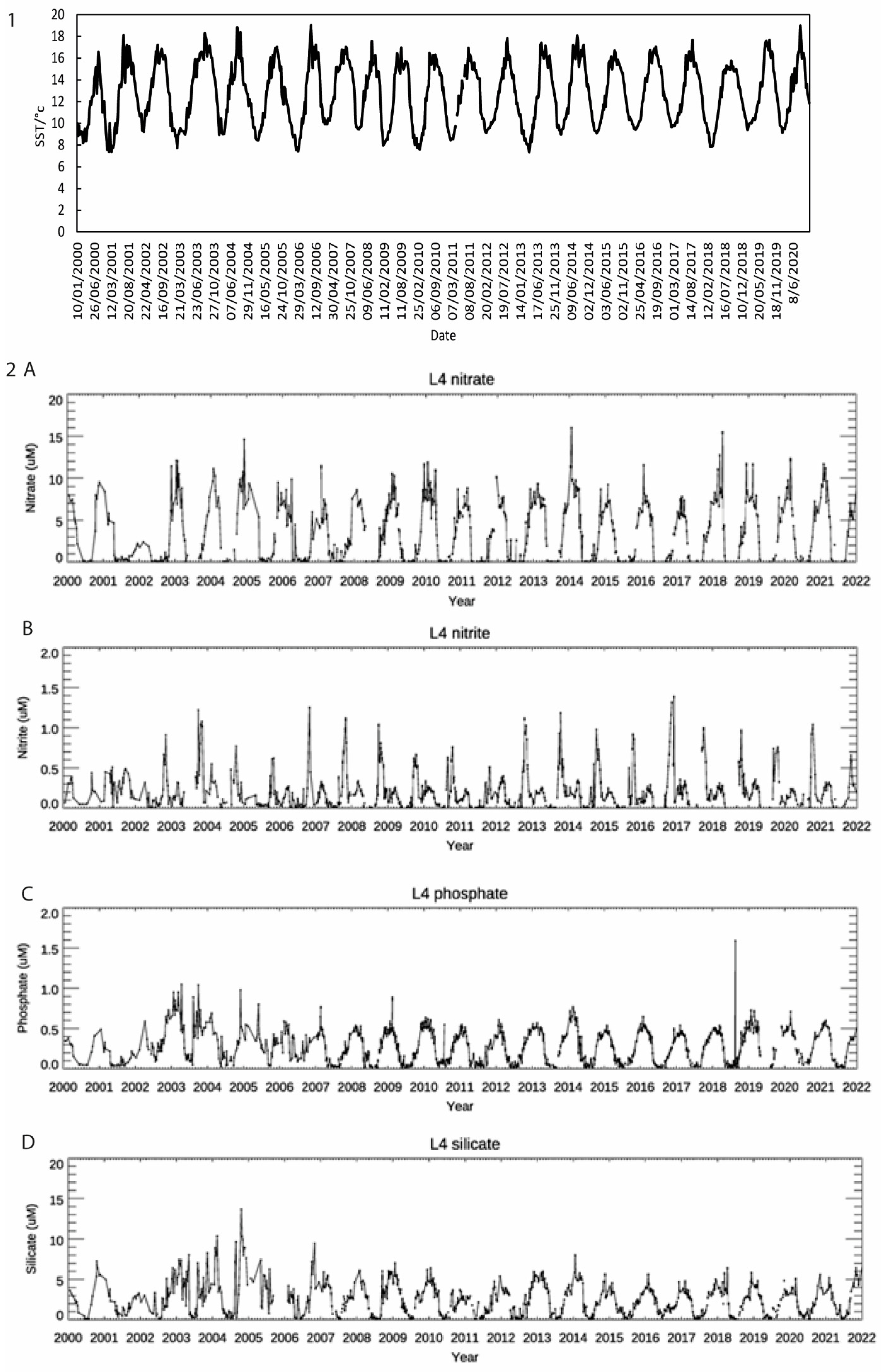
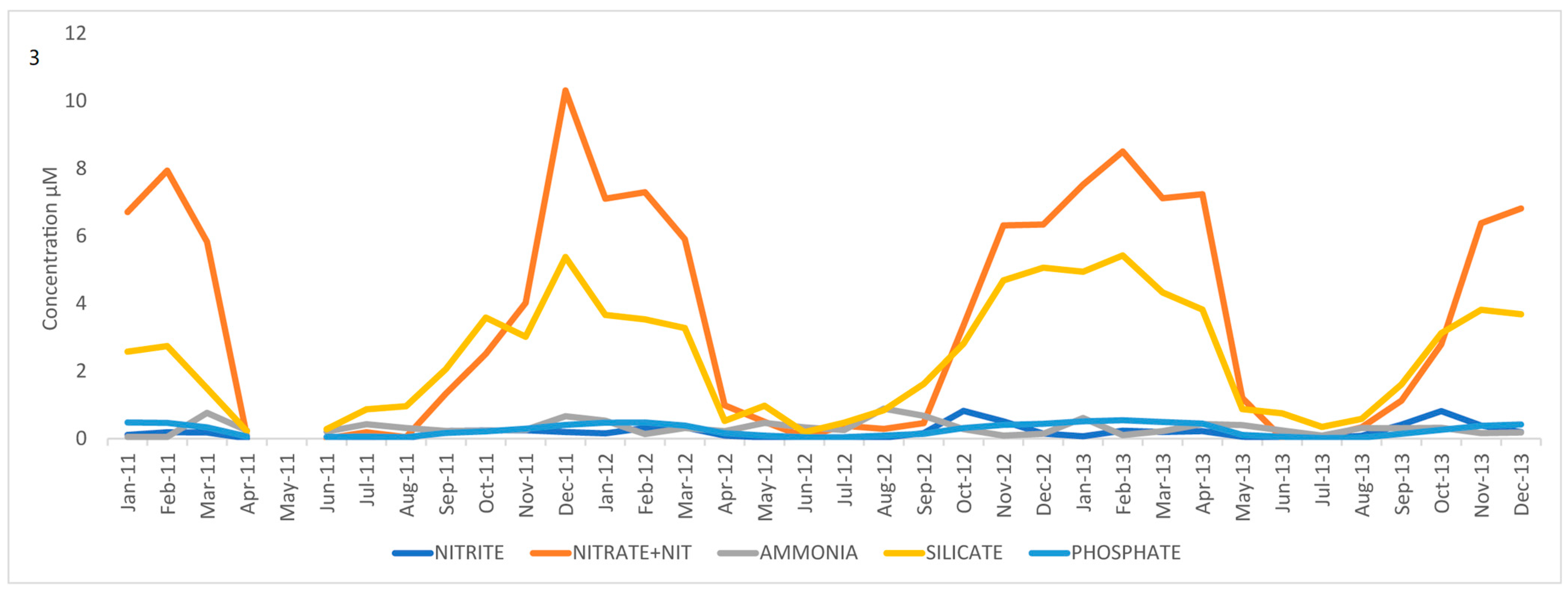
3.1. Nutrient and SST Trends from WCO_L4

The average baseline SST between 2000–2020 was 12.73 °C (7.35–19.04 °C), with the following seasonal averages and ranges: winter 10.14 °C (7.37–13.21 °C); Spring 10.16 °C (7.35–14.23 °C); summer 15.23 °C (11.54–19.04 °C) and autumn 14.83 °C (11.01 to 18.39 °C) SST had a single annual cycle (Figure 2, panel 1). Average annual temperatures from 2011–2013 were similar to the 20-year baseline at 12.48 °C. Seasonal averages of Winter, Spring, Summer and Autumn from 2011–2013 were 10.06 °C, 9.86 °C, 14.98 °C and 14.64 °C respectively, showing cooler summer than the 20-year average. In 2011, a cooler winter SST of 9.43 °C led to warmer than average spring at 10.33 °C. All 2012 there was a warmer than average summer SST at 15.02 °C whilst SST in the Spring of 2013 was cooler at 8.75 °C.

Nutrient cycles over 21 years (see Figure 2, panel 2) revealed an overall repeating single annual cycle for all the nutrients, peaking over the winter and at their lowest levels during the summer months. There are also point increases during the summer months due to occasionally increased river run-off, but the overall annual trends are similar. The 21-year baseline nutrient summer average levels (June–August) (see Table S12) were as follows: nitrite and nitrate (0.02 µM), ammonia (0.13 µM), silicate (0.25 µM) and phosphate (0.06 µM). Summer nutrient depletion levels varied each year, occurring from April–June in 2011, extended from April to September in 2012 and June–August in 2013 (Figure 2, panel 3). In 2011, annual average silicate levels were between two-thirds to two times lower than it’s equivalent 21-year average baseline levels. The most pronounced change in 2011 was winter (December–February) ammonia levels which were four times lower than the 21-year winter average but replenished in the summer. In 2012 and 2013, summer nitrite and nitrate levels were between 4.5–11 times higher than the corresponding 21-year average (Table S12). It should be noted the ammonia cycle is less clear than other nutrients and is more difficult to interpret as part of the time series, so it was treated differently and is prone to contamination.

3.2. HRM and Quantitative Real-Time PCR Assay Performance for Potentially Harmful Algae Taxa

Quantitative real-time PCR (qRT-PCR) combined with HRM was developed for four harmful algae species Pseudo-nitzschia delicatissima, Pseudo-nitzschia fraudulenta and Pseudo-nitzschia multiseries and finally Aureococcus anophagefferens. Only P. delicatissima and A. anophagefferens assays produced results of sufficient quality for the years 2011–2013 and 2011–2012, respectively. All HRM melt-curves of the PCR products from standards and positive controls match those with environmental (see File S2). Sequencing confirmed the P. fraudulenta HRM-qRT-PCR ITS2 product was specific for the positive genomic control (Genbank accession, LN873237) and in the WaMS E4_5.1/WS12 DNA sample (Genbank accession, LN873238) by Blastn comparison method [44]. The identity of the P. multiseries genomic control (Pm12) qRT-PCR product was confirmed (accession number OP504083) but not for WaMS environmental samples. The positive genomic DNA control qRT-PCR ITS1 product for P. delicatissima assay confirmed it’s identity (Genbank accession, OM350397). The qRT-PCR product from A. anophagefferens from three WaMS samples E4_10_11 (1) or WS32, E1_12_11 or WS34 and E1_2_12 or WS39 confirmed species-specific detection (Genbank accession numbers OP484337-OP484339 respectively).

All three PD qRT-PCR reactions were of sufficient quality (Table 3) for quantification and calculation of cell concentrations, as described in File S2. Table 3 shows P. delicatissima 2011–2013 was of sufficient quality for seasonal pattern assessment, despite PD2011 being 3% lower than the threshold, as it’s Ct values were not significantly different from other PD runs ((p = 0.153) at the 5% level. For A. anophagefferens assays, run AA2012 was not statistically different from those of run AA2012 using a student-s t-test (two-sided, unequal variance) p = 0.392 at the 5% level, so it was included in the further analysis, but the AA2013 runs failed so were excluded.

3.3. Seasonal Patterns of Potential Harmful Algae Species in the WaMS Samples by HRM-qRT-PCR

The three Pseudo-nitzschia species measured from the WaMS survey show contrasting patterns of occurrence Pseudo-nitzschia fraudulenta was present in 27 samples: less frequent in 2011 with only eight positive occurrences, and none in March and December, compared to 19 positive samples in all months in 2012. Although the assay was not quantitative, the levels of P. fraudulenta were 10-fold higher relative to other values in April 2011, which was not observed in 2012. P. multiseries was not found in any WaMS sample tested in 2011–2012. WCO L4 P. delicatissima complex microscopic concentrations (Figure 3A) occurred in May–July 2011, peaking in June 2011, and a denser growth appeared in July–October 2013 (Figure 3B). By contrast, WaMS qRT-PCR-measured Pseudo-nitzschia delicatissima only appeared in 2011 and was barely present in the autumn/winter of 2012/13), with peak abundances in February–May of 2011 (Figure 3B). Both analyses showed reduced presence in 2012, although WaMS samples were missing in the key Spring months of April 2012 and March–April 2013, which may have biased the pattern. P. seriata and P. pungens made up a negligible portion of the Pseudo-nitzschia community by microscopy (Figure 3A). The CPR survey revealed the Pseudo-nitzschia delicatissima complex earlier in March, similar to WaMS, and additionally in May–July 2011. Unlike WaMS and WCO L4, it showed both species complex in 2012 and similar P. delicatissima growth period in 2013 except two months later than that of WCO L4 and an additional period in May 2013. The difference in growth periods in these two microscopy datasets indicates variable localized growth responses.

Average cell numbers of A. anophagefferens from WaMS samples in July 2011 were significantly elevated compared to all other dates from 2011 to mid-2013. Station (E5_7_11) at 11 × 10⁹ cells/mL revealed peak abundance (see Table S9a,b). However, these values were above the maximum standard curve values of 4 × 10⁶ cells/mL and so not accurate. Moderately elevated cell concentrations were observed in September, October and December 2011 at 44, 160 and 503 cells/mL, respectively. No detectable A. anophagefferens was observed in 2012, although the gaps in sampling may have missed key growth periods. There was little preference for station location occurrence. The HTS survey revealed the presence of this species in autumn and winter but not July, indicating incomplete detection in the HTS survey.

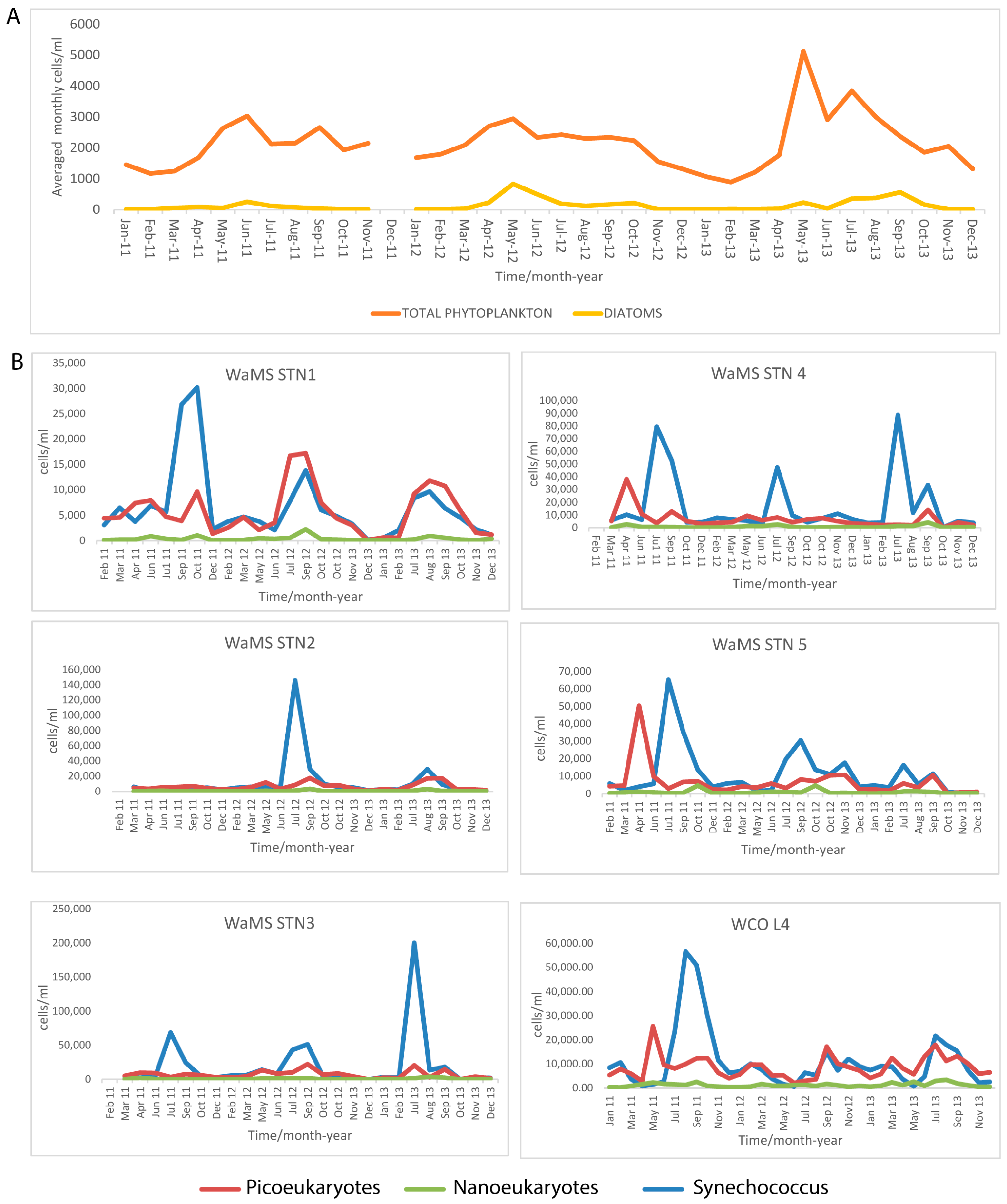
3.4. Phytoplankton Seasonal Trends in the Western Channel from Microscopy, FC from WaMS and WCO L4 Samples

To determine if phytoplankton groups shared similar drivers to the larger phytoplankton community assemblages, the seasonal profiles of larger microscopically measured phytoplankton (~20–200 µm) from WCO-L4 and smaller phytoplankton observed by FC in WaMS and WCO-L4 samples less than 10 µm were plotted (Figure 4).

The diatoms followed a similar pattern to the total phytoplankton, with elevated growth in the spring and autumn, except in 2013, with an autumn peak starting earlier in summer (Figure 4A). Phytoplankton growth was more even in 2012. Unfortunately, no corresponding WaMS flow cytometry data were available for May 2013 for comparison. Picoplankton and Synechococcus (Figure 4B) did not follow these trends. In 2013 diatoms and microscopically measured P. delicatissima species-complex (Figure 3A) showed a single extended summer–autumn growth period, as did nanoeukaryotes, in contrast to phytoplankton that peaked in growth earlier. CPR Pseudo-nitzschia occurrence (Figure 3B) did not match that of total phytoplankton in 2013.

FC-measured Picoeukaryotes abundances from WaMS samples averaged at 6500 cells/mL and numerically dominated nanoeukaryotes (average 689 cells/mL) with variable seasonal patterns per station (Figure 4B) and no clear seasonal cycle except for station 1. Both Synechococcus and picoeukaryotes were similar in abundance in near-coastal environments (WaMS station 1, 5 and WCO L4), whereas mid-channel, Synechococcus numerically dominated in excess of 200,000 cells/mL at station 3 in 2013. The seasonal profile of Synechococcus varied per station and normally occurred once a year, but occasionally a second distinct growth period was observed at stations 4 and 5. The A. anophagefferens high-density growth in July 2011 occurred with that of Synechococcus but just after one of the largest picoeukaryote bloom reaching. Microscopic total phytoplankton counts were of the same order as nanoeukaryotes.

Comparing FC patterns with size-based HTS-derived taxa can provide some insight into phytoplankton taxa assemblages present in pico- or nanophytoplankton groups (Figure 5B, Table S5). The Chloroplastida mostly belonged to pico-sized mamielliophyceae and occurred year-round, although at greater proportions in the spring of 2011 (WS3-WS13). Unusually dinoflagellates belonging to Gymnophycidae are present all year but more so in summer. In Figure 6C, some of these were further identified as Karlodinium in WS16 and WS18, which can be as small as 7 µm. The late spring brought nanoeukaryotes Prymnesiophyceae (including Phaeocystis and Emiliania, Coronoshaera) and potentially unidentified dinoflagellates within the nanoeukaryotes. The summer phytoplankton community showed a greater proportion of nanoeukaryote-sized Gymnophycidae and Stramenopiles (WS14−23). The autumn (WS24−33) phytoplankton diversity was mixed with the nanoeukaryotes Prymnesiales, Phaeocystis, Cryptophytes and potentially nano-sized dinoflagellates. In the winter of 2011/12 (WS34−43), the phytoplankton was a mix of picoplanktonic Chloroplastida, Cryptophya and potentially smaller Gymnodiniphycidae.

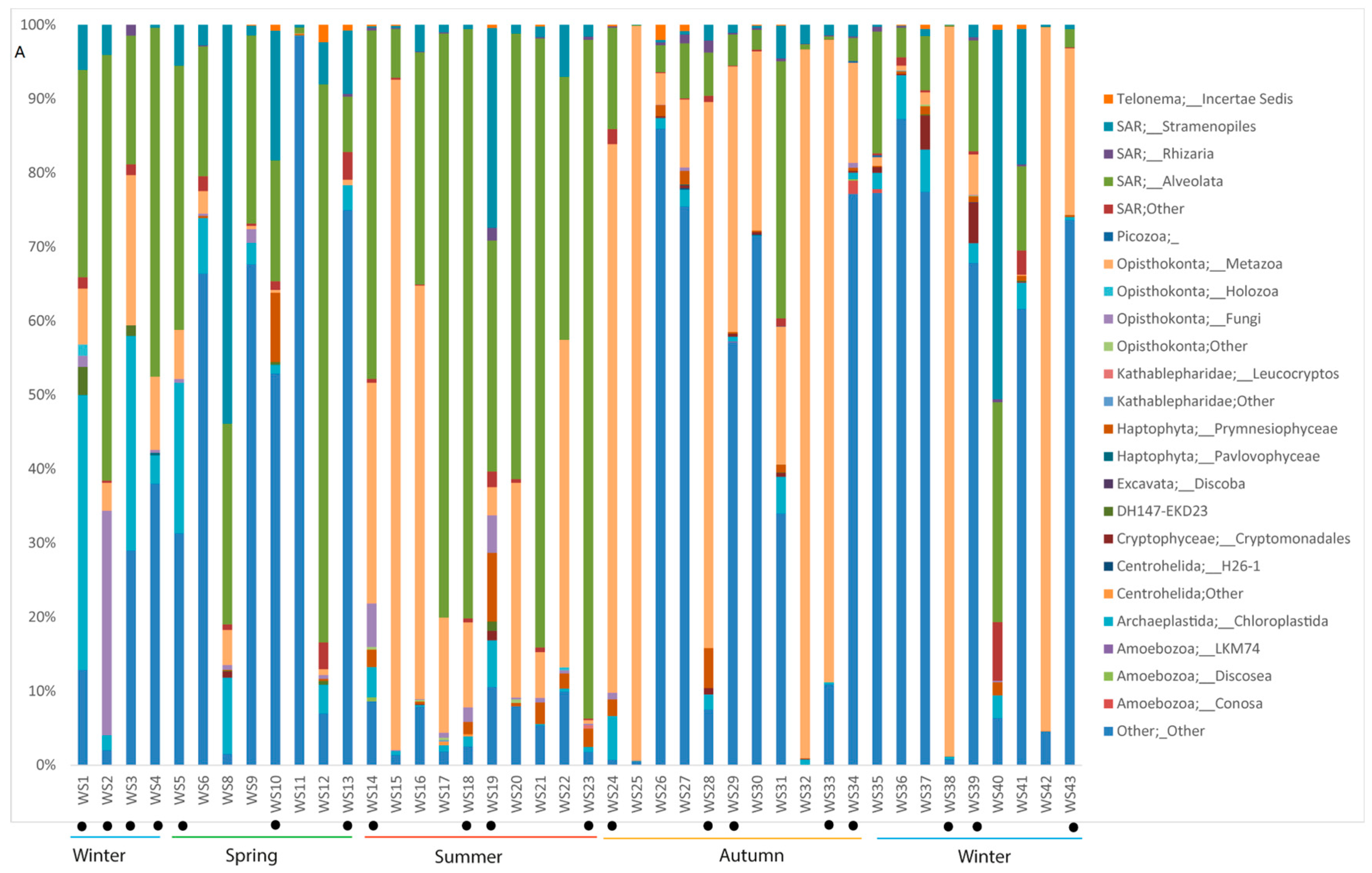
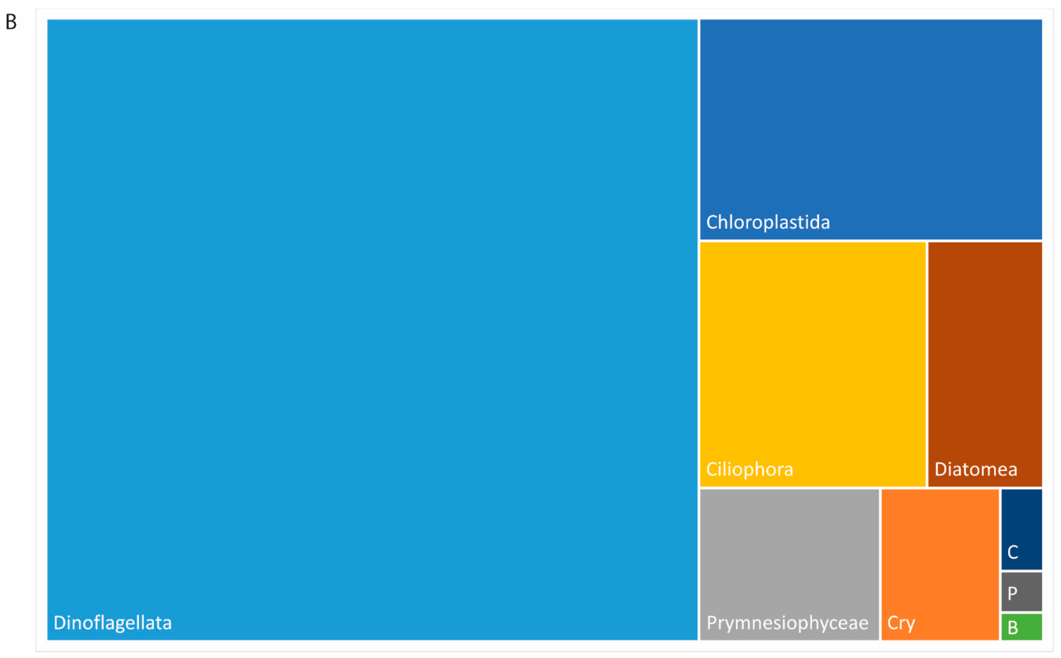
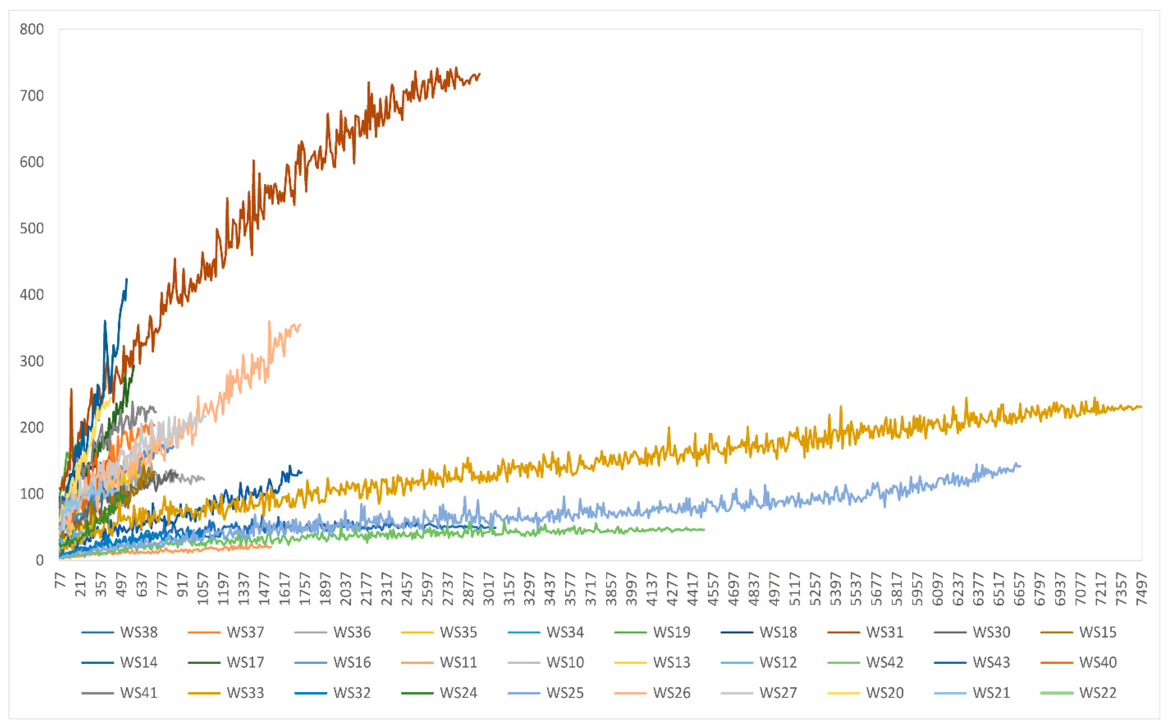
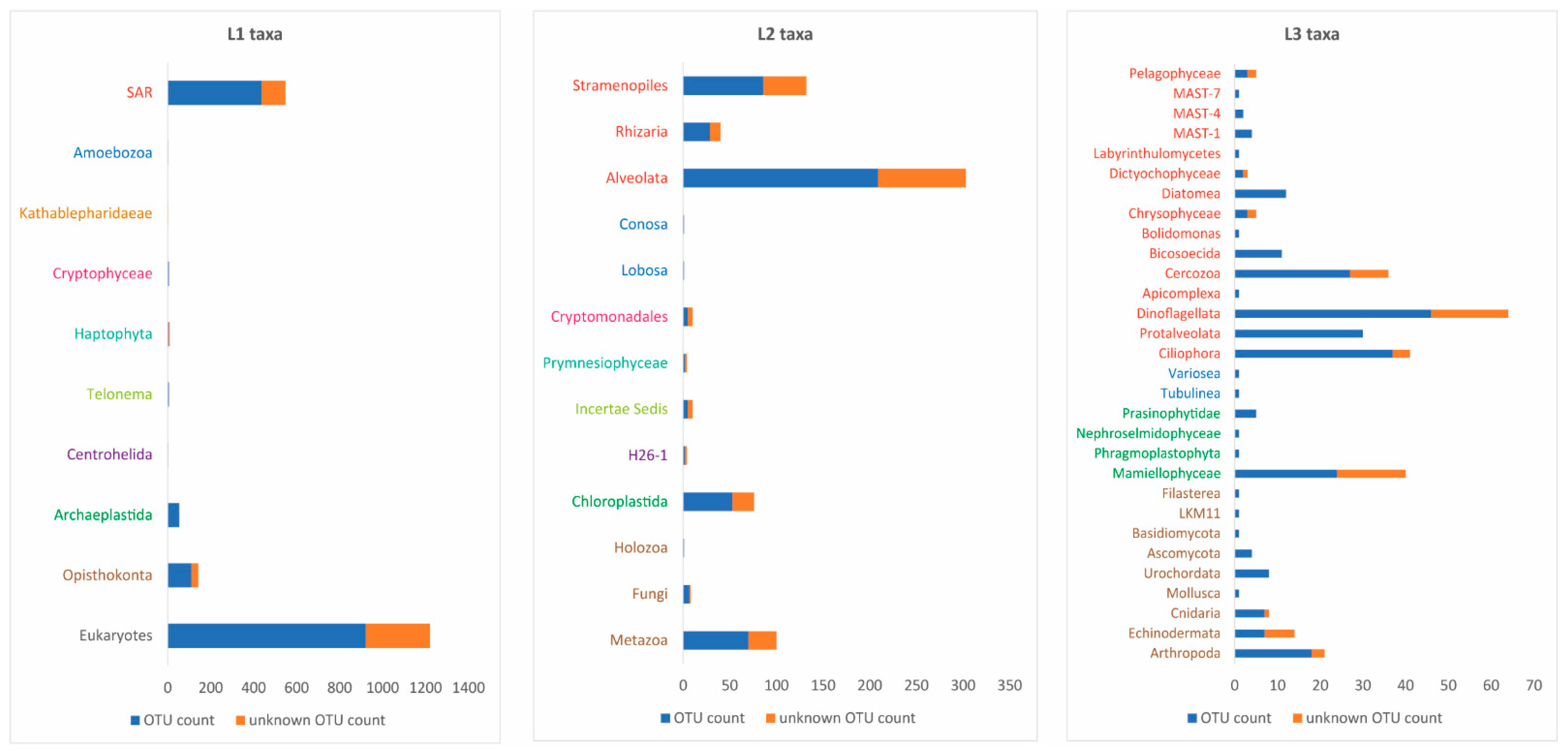
3.5. Plankton Diversity Trends from HTS of Partial 18S rDNA PCR Products from WaMS Samples, WS1−43

After quality filtering and clustering, the total number of reads (DNA sequences) from the combined samples was 49,033, ranging from 69–7500, with a mean of 1167.5 and median of 692 reads per sample (see

Table 4. OTU table count of reads from WaMS sample between 2011–2012. Y: year, M: month, SR: sequence run (run 1 was carried out first and reported in Stern et al., 2015), #: number, PDM: Phylogenetic distance whole tree mean, C1M: Chao I mean, SM: Shannon mean, +/−M: above/below the mean.

Y	M	SR	#/Sample	# OTU	+/− M	Above/Below Median	PDM	C1M	SM
2011	2	1	WS1	132	−1035.452	−560	4.867548	36.0	24.100
2011	2	1	WS2	346	−821.452	−346	1.6509	22.0	9.300
2011	3	1	WS3	69	−1098.452	−623	4.633776	93.1	24.500
2011	3	1	WS4	263	−904.452	−429	1.586147	9.5	7.200
2011	4	1	WS5	182	−985.452	−510	2.120118	39.8	18.600
2011	4	1	WS6	655	−512.452	−37	3.218702	29.3	14.900
2011	4	1	WS8	930	−237.452	238	1.08946	15.7	9.500
2011	4	1	WS9	924	−243.452	232	0.78551	9.9	6.400
2011	5	1	WS10	257	−910.452	−435	0.68059	22.0	12.400
2011	5	1	WS11	1535	367.548	843	0.154481	2.7	2.500
2011	5	1	WS12	386	−781.452	−306	1.175051	23.2	14.100
2011	5	1	WS13	268	−899.452	−424	2.10681	27.6	15.100
2011	6	2	WS14	544	−623.452	−148	1.46735	62.5	23.900
2011	6	2	WS15	729	−438.452	37	1.561149	23.6	13.600
2011	6	2	WS16	861	−306.452	169	2.271352	56.7	25.300
2011	6	2	WS17	592	−575.452	−100	2.49747	43.4	20.900
2011	6	2	WS18	358	−809.452	−334	3.344375	74.0	25.200
2011	7	2	WS19	237	−930.452	−455	3.779641	105.0	35.700
2011	7	2	WS20	427	−740.452	−265	1.589128	32.9	27.300
2011	7	2	WS21	484	−683.452	−208	1.889013	48.0	17.100
2011	7	2	WS22	242	−925.452	−450	2.368124	57.5	18.400
2011	7	2	WS23	445	−722.452	−247	0.71281	38.0	15.000
2011	9	2	WS24	540	−627.452	−152	0.650258	22.1	12.500
2011	9	2	WS25	6674	5506.548	5982	0.319075	4.5	2.900
2011	9	2	WS26	1734	566.548	1042	1.622526	29.2	11.400
2011	9	2	WS27	1080	−87.452	388	1.786829	32.9	14.200
2011	9	2	WS28	240	−927.452	−452	3.088336	79.0	24.000
2011	10	2	WS29	928	−239.452	236	2.057396	39.3	16.000
2011	10	2	WS30	893	−274.452	201	0.256501	36.7	12.100
2011	10	2	WS31	2966	1798.548	2274	2.601002	89.1	31.000
2011	10	2	WS32	1175	7.548	483	0.316267	7.1	4.300
2011	10	2	WS33	7500	6332.548	6808	0.431583	12.9	6.500
2011	12	2	WS34	451	−716.452	−241	0.772125	26.0	11.700
2011	12	2	WS35	766	−401.452	74	1.965868	51.0	13.100
2011	12	2	WS36	1072	−95.452	380	1.2185	20.4	9.800
2011	12	2	WS37	736	−431.452	44	2.471535	25.9	13.400
2011	12	2	WS38	3072	1904.548	2380	0.046794	4.0	3.200
2012	2	2	WS39	902	−265.452	210	2.747683	83.8	18.600
2012	2	2	WS40	455	−712.452	−237	0.916246	23.0	13.500
2012	2	2	WS41	738	−429.452	46	1.699598	66.8	19.200
2012	2	2	WS42	4505	3337.548	3813	0	4.4	3.500
2012	2	2	WS43	1740	572.548	1048	0.67496	10.8	7.200
			Total	49,033

). Read and OTU distributions were unequal across samples, and the first sequencing run showed poorer OTU counts compared to the second. Measures of alpha diversity by Chao1 rarefaction curves (Figure 7, Table 4) confirmed this and suggested the planktonic community was incompletely sampled, with reads for each sample failing to reach plateaus (Figure 7). Due to the bias, it is likely rare taxa are not represented in sequencing run 1, and subsequently, any community analysis (beta diversity) would be likely to be biased. WS7 HTS had failed, as previously identified [19].

Taxa assignments by UCLUST at level 3 (class level or equivalent, Table S2) all major eukaryotic lineages were observed from February 2011–February 2012, though most groups were relatively rare (Figure 5A). The dominant taxonomic groups were uncultured eukaryotes (34%), Metazoa (26%) and Alveolates (25%). A significant minority consisted of Stramenopiles at 6% and Chloroplastida at 4% (see Table S2). Rare taxa contributed just 5% of total reads, but most of the diversity covered 19/24 taxa, while a majority of the dataset (95%) corresponded to reads shared among five taxa (see Table S5).

A total of 50 photosynthetic taxa (summarized in Figure 5B) were present from 2011–2012 in WaMS samples, most in the pico- to nano-size range (see Table S5). Whilst sample read numbers were uneven, average seasonal phytoplankton taxa present revealed less phytoplankton in spring (average 6.8) and winter (average 9.7) compared to summer (average 12) and autumn (average 12.4). Phytoplankton taxa diversity was greater at summer near-coastal stations compared to open water, whilst autumn open-water stations were more diverse than near-coastal counterparts. Less unknown taxa were found in the summer and were dominated by Alveolata (samples WS14−23), including Gymnophycidae and Peridiniphycidae (Figure 5B, Table S5). The proportions of Chloroplastida were present year-round and relatively higher in the winter, spring and autumn of 2011. Prymnesiophyceae Haptophytes occurred year-round, whilst Pavlovophyceae were rare. Proportions of these taxa (Table S2) differed from a WaMS HTS survey (Stern et al., 2015) of February-May 2011 (WS1−6, 8–13) because of the inclusion of metazoans, different output categories (24 here versus 11 in the study of Stern et al., 2015) and bioinformatic pipeline. This made direct comparisons difficult. Nevertheless, Alveolata were prominent in all samples and Chloroplastida in the winter and spring.

Diversity assessments using the RDP classified dataset were similar to UCLUST (see Figure 8), although with a different taxonomic classification. However, this method provided diversity counts at each taxonomic level. A third (446/922) of Eukaryotic OTUs were unidentifiable. The other two-thirds belonged to the SAR supergroup or Opisthokonta in line with the UCLUST output. Level 3 OTUs (262) equivalent to phylum to class (Figure 8) belonged to crustacean arthropods (7%), Mamiellophyceae (9%), with 53% consisting of five alveolate groups (Ciliophora, Protalveolata, Dinoflagellata and Cecozoa). Stramenopiles (mainly Diatomea and Bicosoecida) represented 9% of OTUs. The RDP approach provided better resolution for selected taxa with 16 OTUs identifiable to genus level.

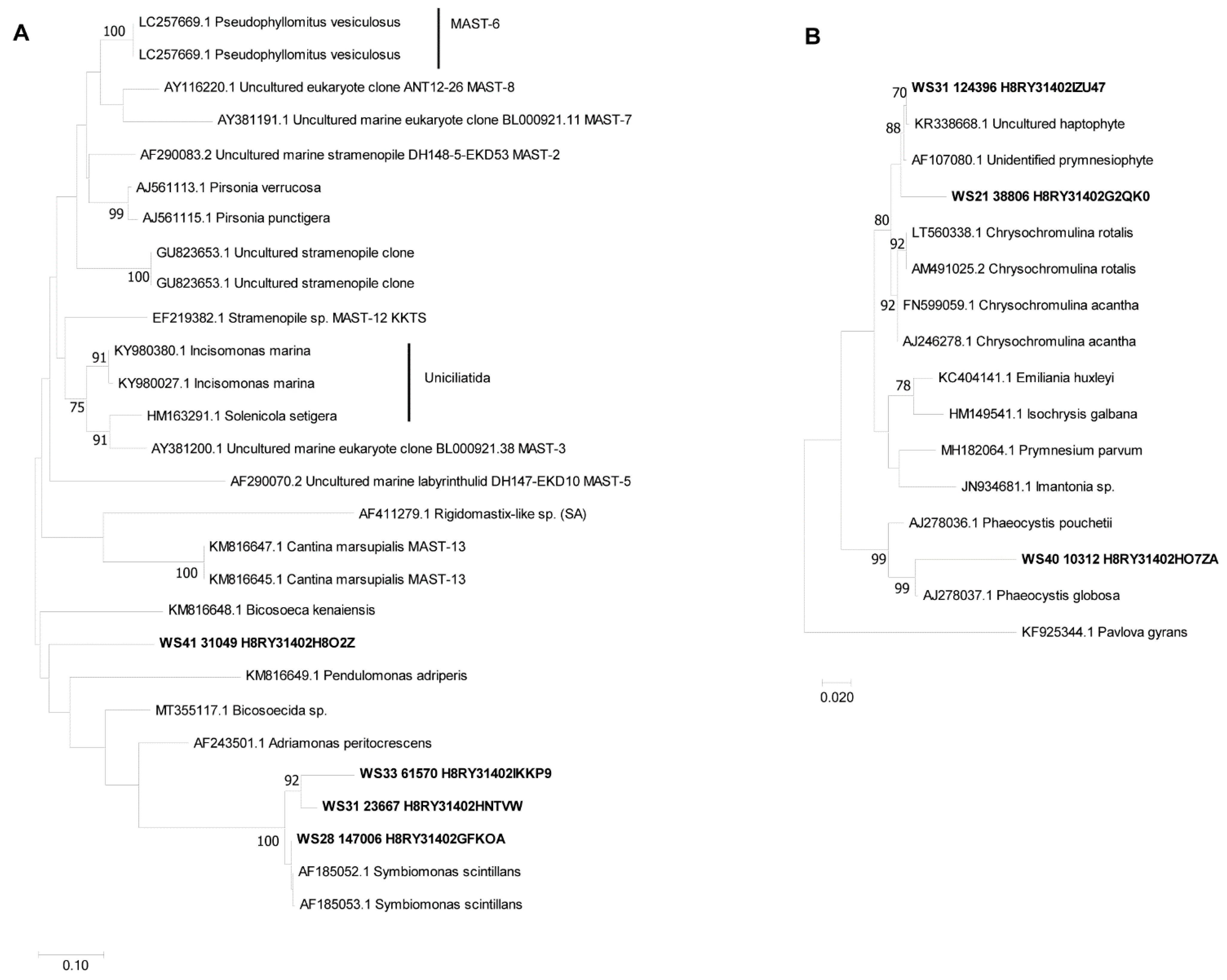
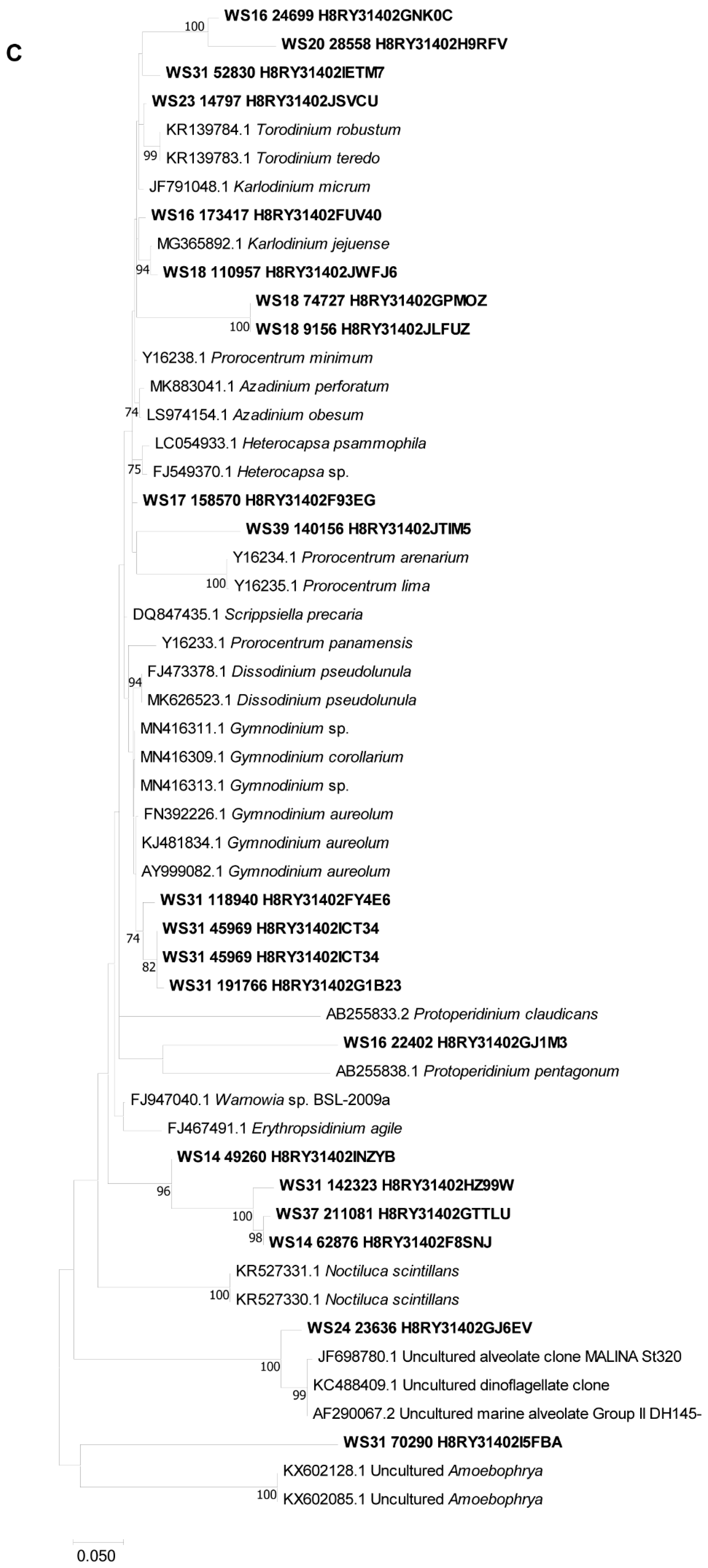
3.6. Phylogenetic Analysis of Partial 18S rDNA Reads of WaMS Samples, WS1−43

Phylogenetic analysis was used to improve the identity of poorly resolved plankton taxa, the dinoflagellates, haptophytes and heterotrophic MAST group from a selection of reads from the HTS survey (Figure 6). Despite the short read size, taxa were able to be identified to the genera level based on known publicly available taxa clustering with them, although with low confidence (Figure 6). Within the MAST group (Figure 6A), a poorly characterized, challenging group, identification was poor except for reads that clustered with Symbiomonas. The Haptophyte phylogeny confirmed the presence of Phaeocystis and an unidentified Prymnesiophyte sister group to Chrysochromulina. Within the dinoflagellates (Figure 6C), several reads clustered with Prorocentrum taxa, which was split into different clades and one OTU grouped with one clade containing the benthic Prorocentrum lima, although with low support. Few OTUs could be identified to genus level with the exception of Karlodinium, Torodinium and Protoperidinium. Three sequences were sister to Toridinium and Karlodinium and likely to belong to Gymnodiniales. Four other sequences were sister to a Gymnodinium species, whilst four others were more deep-branching of unknown origin. Phaeocystsis was the only haptophyte that could be identified. Three other reads were sister to two Chrysochromulina species and could be another of the same species or a related genus. Thus, the use of phylogenetic methods has partially improved taxonomic resolution.

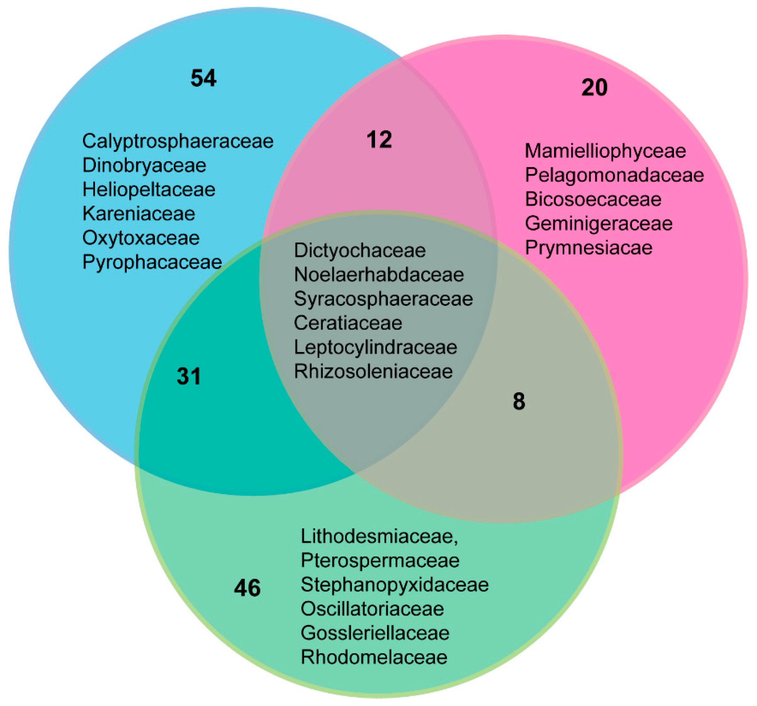
3.7. Comparison of Phytoplankton Diversity from WaMS 18S HTS Survey versus Microscopy Taxonomic Surveys in the Western Channel

WCO L4 phytoplankton microscopic dataset (Table S10) was compared with WaMS genetic (Tables S5 and S6) taxa set and CPR morphological dataset (Table S11) from 2011–2012 to determine the number of common taxa detected from all surveys. Common taxa between each survey are shown in Figure 9. Only six phytoplankton taxa were common to all three surveys. As expected, the CPR and WCO L4 morphological datasets shared the most number of phytoplankton taxa (31 out of a combined 100). Dinoflagellate taxa were most commonly identified in all surveys representing five families and four genera. Only 20 phytoplankton families could be identified from all three surveys, and between eight to 12 of these were shared with microscopic surveys. Phytoplankton taxa under 10 µm were not represented in the morphological datasets such as Pegalophyceae (Aureococcus), Chrysochromulina and Imantionia (of Prymnesiophyceae), Geminigera and Teleaulax (of Cryptophyceae) and Mamiellophyceae (of Chloroplastida). The Flagellate and “Other” taxa categories in the WCO L4 phytoplankton survey had fewer taxa and showed the least overlap with CPR and WaMS genetic taxa, the latter being mostly heterotrophic flagellates. Most OTUs from the WaMS HTS survey belonged to heterotrophic/mixotrophic taxa (73%), with only 38% being autotrophic/mixotrophic (Table S5).

4. Discussion

This study has confirmed how all three surveys detect different and complementary sets of phytoplankton assemblages. For aim 3, there was little overlap with WaMS-genetic and microscopic taxa assemblages, the most extreme being WaMS and CPR phytoplankton. Even in this well-characterized system, many eukaryotes are unknown. Microscopic methods provided high-resolution taxa for hard-shelled phytoplankton taxa, whilst WaMS provided diverse assemblages of soft-bodied and mostly or pico- to nano-sized phytoplankton, even with incomplete diversity captured. This, in turn, complemented the low-resolution FC data, which can detect four to seven aggregated phytoplankton groups but with good size precision, revealing a succession of phytoplankton taxa increasing taxonomic resolution of phytoplankton assemblages. Factors that influenced biodiversity outputs were uneven and incomplete sequences captured in WaMS, gaps in the public sequence database and the limitations of a 300 bp region of 18S rDNA which could only resolve taxa with good reference sequence representation but failed when it was poor, such as in the MAST group. Sample volume is one of the biggest influences on diversity captured; only 50 mL of WaMS samples were used for DNA extractions compared to 200 mL of WCO L4 water and 3 m³ of filtered water on CPR silks, the latter two capturing larger phytoplankton.

Interestingly, most of the taxa found in January to May 2011 of WaMS in our earlier study [19] were present year-round, which would confirm a consistent seed of species that can grow under the right conditions. Previous 18S amplicon sequencing surveys also showed chlorophytes, prymnesiophytes and cryptophytes are major taxa present in the Western channel [19,56] but poorly represented by microscopy.

4.1. Performance of WaMS Sampling for Harmful Algae, Pico- and Nanoplankton Quantification

The WaMS performance showed the most success with the FC detection of cells. This only required 2 mL and best suited this machine’s small volume sampling mechanism and the larger cell densities of small phytoplankton taxa. Whilst the presence of four potentially harmful algae species was successful, their quantification only worked for two species. Most species were at or below the detection threshold of standards, likely due to the small volume of WaMS reducing the number of cells captured. The absolute abundance of Pseudo-nitzschia delicatissima detected by qRT-PCR, although of the same order, differed from its equivalent morphospecies level microscopic counts, sometimes exceeding them. Although the latter encompasses at least six species [57,58], abundances are confounded by the presence of residual Pseudo-nitzschia eDNA-it’s genetic detection without microscopic presence has been reported earlier [59]. Technical issues included variability between qRT-PCR runs, despite the use of the same standards and reagents. Whilst this study used SYBR green assay, which is cheaper, it did impact reaction efficiency by non-specific binding with primer dimers or non-specific products, even in WaMS samples where DNA was extracted identically and tested at the same time. This may have arisen from environmental sample contaminants. Nevertheless, these issues can be overcome with larger sampling volumes, a baseline methodology qRT-PCR microscopic comparison alongside non-ambiguous phytoplankton species and further optimization to improve reaction efficiency to the level of TaqMan PCR [60] or to use TaqMan PCR assays. Finally, machine error in the WaMS sampler occurred in key months, which negatively impacted this study, mainly due to machine service needs or battery failure. Larger sampling volumes require larger batteries, and there are limitations between payload size for a sampler on most moving marine platforms, including the CPR survey, which are often size restricted to enable them to be autonomous or to measure other variables. Improvements to battery sizes, sample filters and/or in-situ detectors will reduce barriers to automated sampling on moving platforms.

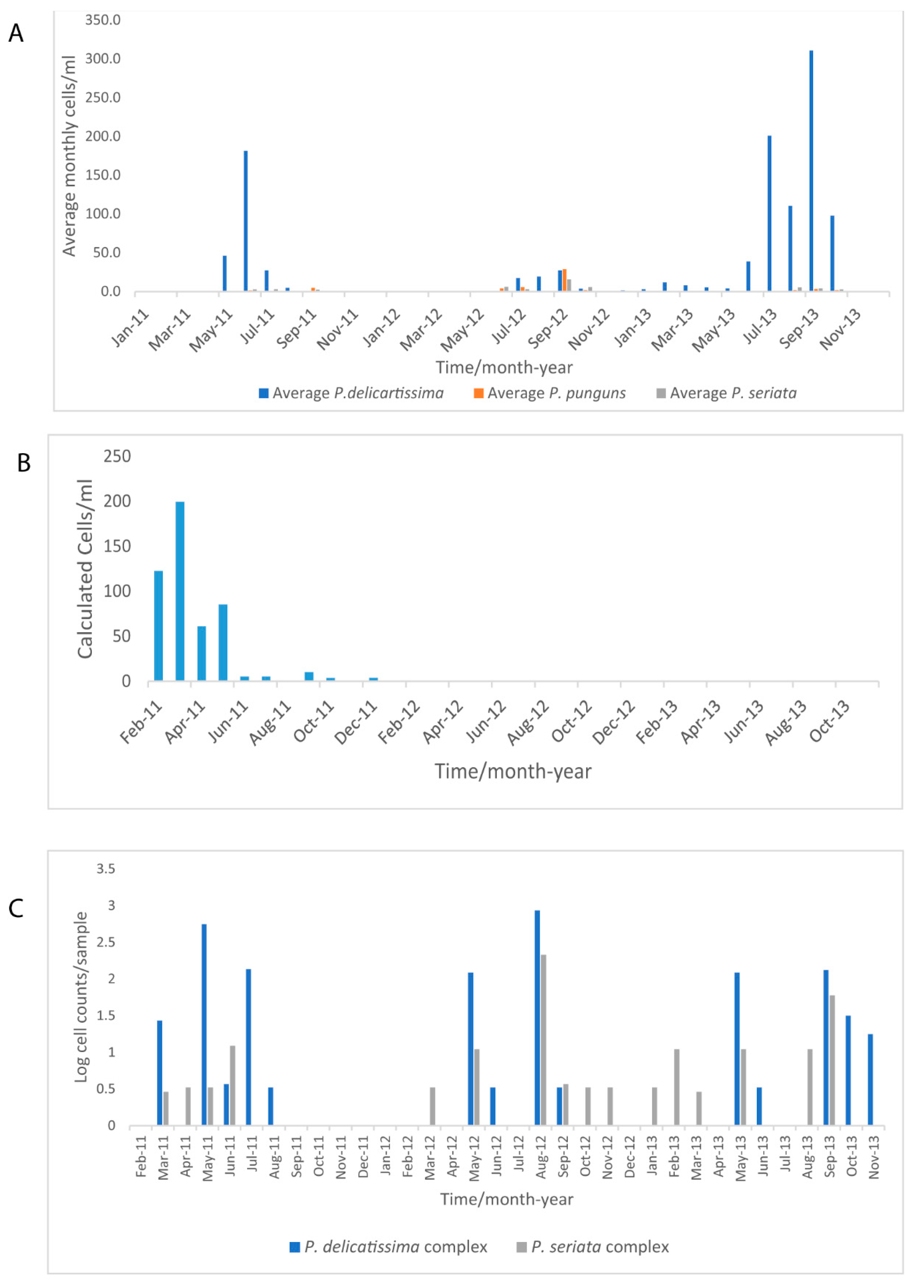
4.2. Seasonal Dynamics of P. delicatissima and A. anophagefferens in Comparison to FC- and Microscopy Measured Phytoplankton Groups

Pico- and nanophytoplankton were reported to account for 48% of carbon fixation at the WCO L4 station [15]. Trends in aggregated size-fractioned phytoplankton groups measured by FC in WaMS samples revealed great regional variation indicating sensitivity to local conditions. Atlantic-influenced mid-channel open waters were dominated by Synechococcus in these years with little else, whereas near-coastal WCO-L4 sites and WaMS station 4 are influenced by pulses of riverine output with nutrients [61] and show elevated picoeukaryotes. Here we show these assemblages change by season and region. The presence of winter/spring Chloroplastida is mostly Mamiellophyceae that are adapted into ecogroups, some of which prefer low light conditions in winter [62]. Pico- and nano-eukaryotic abundance is linked to winter nutrient concentrations and also the biomass of Phaeocystis, indicating a biological dependence on other phytoplankton [15]. By contrast, A. anophagefferens prefers low salinity and higher organic carbon and nitrogenous nutrient conditions [30,63] with a suite of genes that can adapt to low light and elevated organic carbon or nitrogen sources. This higher density growth may have arisen from a pulse of nutrients from riverine influence. In 2011, ammonia levels were unusually relatively elevated in summer which this organism may have been able to utilize [30].

Pseudo-nitzschia detection by HRM-qRT-PCR extended the species resolution of species groups, normally grouped into three microscopic categories. This method of detection was very sensitive to species detection, even if quantification could not be achieved for all species. It revealed different occurrences of Pseudo-nitzschia with the likely toxic P. multiseries being rare to absent, P. fraudulenta of moderate frequency and P. delicatissima most frequently. P. delicatissima species complex is the most abundant at WCO L4 in this and earlier studies [20]. All of these species were more frequent in 2011 compared to 2012/2013. Previous studies Downes-Tettmar [24] narrowed down potential toxin producers to two groups in this region which is now likely to include P. fraudulenta (DA was not associated with P. delicatissima). P. delicatissima was the most directly comparable between WaMS and microscopy surveys. The CPR survey confirmed its early spring occurrence in March, which extended to a February appearance in WaMS samples but not in the corresponding microscopic WCO L4 microscopic survey. The genetic survey shows the early detection of a Pseudo-nitzschia for early warning systems present at all stations, but its rarity in 2012 and 2013 compared to other studies may indicate it was a separate population responding to local growth conditions or that it was not adequately captured. P. delicatissima’s growth profile was different from its corresponding morphospecies, which typically grow in spring and autumn [20]. Local conditions were found to be associated with Pseudo-nitzschia spp. growth on the French coast of the Western Channel [64] that might confirm a highly localized growth pattern. Temperature and nutrients were reported to influence diatoms and P. delicatissima assemblages at WCO station L4 [24,65]. No clear driver is discernable here, but a warmer spring occurred in 2011, which may have benefited P. delicatissima’s growth in 2011. The genetic assays developed [28] and tested here will likely improve monitoring to elucidate conditions that lead to toxin versus non-toxin-producing Pseudo-nitzschia spp.

This study has further advanced the understanding of diversity and individual phytoplankton species responses and how both broader sampling transects provide a greater understanding of local conditions. Nevertheless, it was limited in time to a 5–10 year baseline which could allow statistically reliable links with physicochemical parameters or to biological ones. The WaMS samples series had gaps and used small volumes that hindered direct morphological to genetic species comparisons, in addition to the use of unambiguous species. A direct diversity comparison using an HTS survey from WCO L4 samples at normal or the same volumes as that of WaMS would provide more information on diversity captured by each system and their spatio-temporal distribution.

All these methods provide a complementary approach to the routine monitoring of our seas, covering breadth and depth as outlined in this summary schematic (Figure 10). Most of the organisms detected genetically in WaMS samples are not included in any official assessment of marine plankton health [13] and represent a large portion of biodiversity and primary productivity [15]. Taxa bias can be overcome using blocking oligonucleotides [66] or evenness of taxa representation by primer cocktails [67]. However, long-read high throughput methods can now provide high-resolution genomic and taxonomic diversity assessments at the species or even strain level potentially without bias-inducing amplification step [68]. HTS presence data at high sampling frequencies can be powerful in developing ecological models, such as the prediction of plankton organisms significantly associated with carbon export using metagenomic TARA ocean data [69]. For genetic approaches to be used routinely, a period of comparison for standardization of methods at all stages and the use of common taxonomic reference databases will augment diversity information to effectively monitor phytoplankton more completely [70].

5. Conclusions

Genetically-measured taxa composition measures different communities and complements microscopic observations. The species-level detection of morphologically indistinct taxa often shows different profiles to the aggregate community that provides insights into their habitat preferences and promise as indicators.

References

1. Vincent, F.; Ibarbalz, F.M.; Bowler, C. Global marine phytoplankton revealed by the Tara Oceans expedition. In Advances in Phytoplankton Ecology; Clementson, L.A., Eriksen, R.S., Willis, A., Eds.; Elsevier: Amsterdam, The Netherlands, 2022; pp. 531–561. [Google Scholar]
2. Falkowski, P.G.; Raven, J.A. Aquatic photosynthesis; Princeton University Press: Princeton, NJ, USA, 2013. [Google Scholar]
3. Falkowski, P. Ocean Science: The power of plankton. Nature 2012, 483, S17–S20. [Google Scholar] [CrossRef]
4. Finkel, Z.V.; Beardall, J.; Flynn, K.J.; Quigg, A.; Rees, T.A.V.; Raven, J.A. Phytoplankton in a changing world: Cell size and elemental stoichiometry. J. Plankton Res. 2009, 32, 119–137. [Google Scholar] [CrossRef] [Green Version]
5. Cardoso, A.C.; Hanke, G.; Hoeppffner, N.; Palialexis, A.; Somma, F.; Stips, A.; Teixeira, H.; Tempera, F.; Tornero, V. D1 Biological Diversity. Available online: https://mcc.jrc.ec.europa.eu/main/dev.py?N=19&O=118&titre_chap=D1%20Biological%20diversity (accessed on 16 September 2022).
6. Miloslavich, P.; Bax, N.J.; Simmons, S.E.; Klein, E.; Appeltans, W.; Aburto-Oropeza, O.; Andersen Garcia, M.; Batten, S.D.; Benedetti-Cecchi, L.; Checkley, D.M., Jr.; et al. Essential ocean variables for global sustained observations of biodiversity and ecosystem changes. Glob. Chang. Biol. 2018, 24, 2416–2433. [Google Scholar]
7. Brondizio, E.S.; Settele, J.; Díaz, S.; Ngo, H.T. Global Assessment Report on Biodiversity and Ecosystem Services; Intergovernmental Science-Policy Platform on Biodiversity and Ecosystem Services: Bonn, Germany, 2019. [Google Scholar]
8. Vargas, C.d.; Audic, S.; Henry, N.; Decelle, J.; Mahé, F.; Logares, R.; Lara, E.; Berney, C.; Bescot, N.L.; Probert, I.; et al. Eukaryotic plankton diversity in the sunlit ocean. Science 2015, 348, 1261605. [Google Scholar] [CrossRef] [Green Version]
9. Hällfors, G.; Melvasalo, T.; Niemi, A.; Viljamaa, H. Effect of different fixatives and preservatives on phytoplankton counts. Pub. Water Res. Inst. 1979, 34, 25–34. [Google Scholar]
10. Sosik, H.M.; Olson, R.J.; Armbrust, E.V. Flow Cytometry in Phytoplankton Research. In Chlorophyll a Fluorescence in Aquatic Sciences: Methods and Applications; Suggett, D.J., Prášil, O., Borowitzka, M.A., Eds.; Springer: Dordrecht, The Netherlands, 2010; pp. 171–185. [Google Scholar] [CrossRef]
11. Xiao, X.; Sogge, H.; Lagesen, K.; Tooming-Klunderud, A.; Jakobsen, K.S.; Rohrlack, T. Use of High Throughput Sequencing and Light Microscopy Show Contrasting Results in a Study of Phytoplankton Occurrence in a Freshwater Environment. PLoS ONE 2014, 9, e106510. [Google Scholar]
12. Godhe, A.; Asplund, M.E.; Härnstörm, K.; Saravanan, V.; Tyagi, A.; Karunasagar, I. Quantification of Diatom and Dinoflagellate Biomasses in Coastal Marine Seawater Samples by Real-Time PCR. Appl. Environ. Microbiol. 2008, 74, 7174–7182. [Google Scholar]
13. McQuatters-Gollop, A.; Guérin, L.; Arroyo, N.L.; Aubert, A.; Artigas, L.F.; Bedford, J.; Corcoran, E.; Dierschke, V.; Elliott, S.A.M.; Geelhoed, S.C.V.; et al. Assessing the state of marine biodiversity in the Northeast Atlantic. Ecol. Indic. 2022, 141, 109148. [Google Scholar]
14. Uncles, R.J.; Stephens, J.A.; Harris, C. Physical processes in a coupled bay–estuary coastal system: Whitsand Bay and Plymouth Sound. Prog. Oceanogr. 2015, 137, 360–384. [Google Scholar]
15. Barnes, M.K.; Tilstone, G.H.; Suggett, D.J.; Widdicombe, C.E.; Bruun, J.; Martinez-Vicente, V.; Smyth, T.J. Temporal variability in total, micro- and nano-phytoplankton primary production at a coastal site in the Western English Channel. Prog. Oceanogr. 2015, 137, 470–483. [Google Scholar]
16. Napoléon, C.; Fiant, L.; Raimbault, V.; Riou, P.; Claquin, P. Dynamics of phytoplankton diversity structure and primary productivity in the English Channel. Mar. Ecol. Prog. Ser. 2014, 505, 49–64. [Google Scholar]
17. Richardson, A.J.; Walne, A.W.; John, A.W.G.; Jonas, T.D.; Lindley, J.A.; Sims, D.W.; Stevens, D.; Witt, M. Using continuous plankton recorder data. Prog. Oceanogr. 2006, 68, 27–74. [Google Scholar]
18. Southward, A.J.; Langmead, O.; Hardman-Mountford, N.J.; Aiken, J.; Boalch, G.T.; Dando, P.R.; Genner, M.J.; Joint, I.; Kendall, M.A.; Halliday, N.C.; et al. Long-Term Oceanographic and Ecological Research in the Western English Channel. Adv. Mar. Biol. 2005, 47, 1–105. [Google Scholar]
19. Stern, R.F.; Picard, K.; Hamilton, K.M.; Walne, A.; McQuatters-Gollop, A.; Mills, D.; Edwards, M. An automated water sampler from Ships of Opportunity detects new boundaries of marine microbial biodiversity. Prog. Oceanogr. 2015, 137, 409–420. [Google Scholar] [CrossRef]
20. Widdicombe, C.; Eloire, D.; Harbour, D.; Harris, R.; Somerfield, P. Long-term phytoplankton community dynamics in the Western English Channel. J. Plankton Res. 2010, 32, 643–655. [Google Scholar]
21. Hinder, S.L.; Hays, G.C.; Edwards, M.; Roberts, E.C.; Walne, A.W.; Gravenor, M.B. Changes in marine dinoflagellate and diatom abundance under climate change. Nat. Clim. Chang. 2012, 2, 271–275. [Google Scholar] [CrossRef]
22. Bates, S.S.; Hubbard, K.A.; Lundholm, N.; Montresor, M.; Leaw, C.P. Pseudo-nitzschia, Nitzschia, and domoic acid: New research since 2011. Harmful Algae 2018, 79, 3–43. [Google Scholar]
23. Hasle, G.; Lange, C.; Syvertsen, E. A review of Pseudo-nitzschia, with special reference to the Skagerrak, North Atlantic, and adjacent waters. Helgoländer Meeresunters. 1996, 50, 131–175. [Google Scholar]
24. Downes-Tettmar, N.; Rowland, S.; Widdicombe, C.; Woodward, M.; Llewellyn, C. Seasonal variation in Pseudo-nitzschia spp. and domoic acid in the Western English Channel. Cont. Shelf Res. 2013, 53, 40–49. [Google Scholar]
25. Brunson, J.K.; McKinnie, S.M.K.; Chekan, J.R.; McCrow, J.P.; Miles, Z.D.; Bertrand, E.M.; Bielinski, V.A.; Luhavaya, H.; Oborník, M.; Smith, G.J.; et al. Biosynthesis of the neurotoxin domoic acid in a bloom-forming diatom. Science 2018, 361, 1356–1358. [Google Scholar] [CrossRef] [Green Version]
26. Sobrinho, B.F.; De Camargo, L.M.; Sandrini-Neto, L.; Kleemann, C.R.; Machado, E.d.C.; Mafra, L.L. Growth, Toxin Production and Allelopathic Effects of Pseudo-nitzschia multiseries under Iron-Enriched Conditions. Mar. Drugs 2017, 15, 331. [Google Scholar]
27. Downes-Tettmar, N. Factors That Impact Pseudo-nitzschia spp. Occurence, Growth, and Toxin Production. Ph.D. Thesis, University of Plymouth, Plymouth, UK, 2012. [Google Scholar]
28. Andree, K.B.; Fernández-Tejedor, M.; Elandaloussi, L.M.; Quijano-Scheggia, S.; Sampedro, N.; Garcés, E.; Camp, J.; Diogène, J. Quantitative PCR Coupled with Melt Curve Analysis for Detection of Selected Pseudo-nitzschia spp. (Bacillariophyceae) from the Northwestern Mediterranean Sea. Appl. Environ. Microbiol. 2011, 77, 1651–1659. [Google Scholar] [CrossRef] [Green Version]
29. Popels, L.C.; Cary, S.C.; Hutchins, D.A.; Forbes, R.; Pustizzi, F.; Gobler, C.J.; Coyne, K.J. The use of quantitative polymerase chain reaction forthe detection and enumeration of the harmful algaAureococcus anophagef-ferensin environmental samples along the United States East Coast. Limnol. Oceanogr. Methods 2003, 1, 92–102. [Google Scholar]
30. Gobler, C.J.; Berry, D.L.; Dyhrman, S.T.; Wilhelm, S.W.; Salamov, A.; Lobanov, A.V.; Zhang, Y.; Collier, J.L.; Wurch, L.L.; Kustka, A.B.; et al. Niche of harmful alga Aureococcus anophagefferen revealed through ecogenomics. Proc. Natl. Acad. Sci. USA 2011, 108, 4352–4357. [Google Scholar] [CrossRef] [Green Version]
31. Doblin, M.A.; Popels, L.C.; Coyne, K.J.; Hutchins, D.A.; Cary, S.C.; Dobbs, F.C. Transport of the Harmful Bloom Alga Aureococcus anophagefferens by Oceangoing Ships and Coastal Boats. Appl. Environ. Microbiol. 2004, 70, 6495–6500. [Google Scholar] [CrossRef] [Green Version]
32. Throndsen, J. Preservation and storage. In Phytoplankton Manual; Sournia, A., Ed.; UNESCO: Paris, France, 1978; pp. 69–74. [Google Scholar]
33. Becker, S.; Aoyama, M.; Woodward, E.M.S.; Bakker, K.; Coverly, S.; Mahaffey, C.; Tanhua, T. GO-SHIP Repeat Hydrography Nutrient Manual: The Precise and Accurate Determination of Dissolved Inorganic Nutrients in Seawater, Using Continuous Flow Analysis Methods. Front. Mar. Sci. 2020, 7, 581790. [Google Scholar] [CrossRef]
34. Reid, P.C.; Colebrook, J.M.; Matthews, J.B.L.; Aiken, J.; Continuous Plankton Recorder Team. The Continuous Plankton Recorder: Concepts and history, from Plankton Indicator to undulating recorders. Prog. Oceanogr. 2003, 58, 117–173. [Google Scholar]
35. Widdicombe, C.E.; Harbour, D. Phytoplankton Taxonomic Abundance and Biomass Time-Series at Plymouth Station L4 in the Western English Channel, 1992–2020; British Oceanographic Data Centre NOC: Liverpool, UK, 2021. [Google Scholar]
36. Utermöhl, H. Methods of collecting plankton for various purposes are discussed. SIL Commun. 1953–1996 1958, 9, 1–38. [Google Scholar] [CrossRef]
37. Winnepenninckx, B.; Backeljau, T.; De Wachter, R. Extraction of high molecular weight DNA from molluscs. Trends Genet. 1993, 9, 407. [Google Scholar]
38. Walker, C.E. Molecular Identification of Pseudo-nitzschia Species in the English Channel; University of Plymouth: Plymouth, UK, 2014. [Google Scholar]
39. Medlin, L.; Elwood, H.J.; Stickel, S.; Sogin, M.L. The characterization of enzymatically amplified eukaryotic 16s-like rRNA-coding regions. Gene 1988, 71, 491–499. [Google Scholar] [CrossRef] [Green Version]
40. Caporaso, J.G.; Kuczynski, J.; Stombaugh, J.; Bittinger, K.; Bushman, F.D.; Costello, E.K.; Fierer, N.; Gonzalez Pena, A.; Goodrich, J.K.; Gordon, J.I.; et al. QIIME allows analysis of high-throughput community sequencing data. Nat. Methods 2010, 7, 335–336. [Google Scholar] [CrossRef] [Green Version]
41. Edgar, R.C. Search and clustering orders of magnitude faster than BLAST. Bioinformatics 2010, 26, 2460–2461. [Google Scholar] [CrossRef] [Green Version]
42. Wang, Q.; Garrity, G.M.; Tiedje, J.M.; Cole, J.R. Naive Bayesian classifier for rapid assignment of rRNA sequences into the new bacterial taxonomy. Appl. Environ. Microbiol. 2007, 73, 5261–5267. [Google Scholar] [CrossRef] [Green Version]
43. Quast, C.; Pruesse, E.; Yilmaz, P.; Gerken, J.; Schweer, T.; Yarza, P.; Peplies, J.; Glöckner, F.O. The SILVA ribosomal RNA gene database project: Improved data processing and web-based tools. Nucleic Acids Res. 2013, 41, D590–D596. [Google Scholar]
44. Altschul, S.F.; Gish, W.; Miller, W.; Myers, E.W.; Lipman, D.J. Basic local alignment search tool. J. Mol. Biol. 1990, 215, 403–410. [Google Scholar]
45. Hall, T. BioEdit: A user-friendly biological sequence alignment editor and analysis program for Windows 95/98/NT. Nucleic Acids Symp. Ser. 1999, 41, 95–98. [Google Scholar]
46. Tamura, K.; Stecher, G.; Peterson, D.; Filipski, A.; Kumar, S. MEGA6: Molecular Evolutionary Genetics Analysis version 6.0. Mol. Biol. Evol. 2013, 30, 2725–2729. [Google Scholar]
47. Tamura, K.S.G.; Kumar, S. MEGA 11: Molecular Evolutionary Genetics Analysis Version 11. Mol. Biol. Evol. 2021, 38, 3022–3027. [Google Scholar]
48. Skovgaard, A.; Karpov, S.A.; Guillou, L. The Parasitic Dinoflagellates Blastodinium spp. Inhabiting the Gut of Marine, Planktonic Copepods: Morphology, Ecology, and Unrecognized Species Diversity. Front. Microbiol. 2012, 3, 305. [Google Scholar]
49. Steidinger, K.A.; Tangen, K. Dinoflagellates. In Identifying Marine Phytoplankton; Tomas, C.R., Ed.; Academic Press: San Diego, CA, USA, 1997; pp. 387–584. [Google Scholar]
50. Throndsen, J. The planktonic marine flagellates. In Identifying Marine Phytoplankton; Tomas, C.R., Ed.; Academic Press: San Diego, CA, USA, 1997; pp. 633–644. [Google Scholar]
51. Tomas, C.R. (Ed.) Identifying Marine Phytoplankton; Academic Press: San Diego, CA, USA, 1997. [Google Scholar]
52. WoRMS Editorial Board. World Register of Marine Species; VLIZ: Ostend, Belgium, 2022. [Google Scholar]
53. Yilmaz, P.; Parfrey, L.W.; Yarza, P.; Gerken, J.; Pruesse, E.; Quast, C.; Schweer, T.; Peplies, J.; Ludwig, W.; Glöckner, F.O. The SILVA and “All-species Living Tree Project (LTP)” taxonomic frameworks. Nucleic Acids Res. 2014, 42, D643–D648. [Google Scholar]
54. Medin, L. Evolution of the diatoms: Major steps in their evolution and a review of the supporting molecular and morphological evidence. Phycologia 2016, 55, 79–103. [Google Scholar]
55. Guiry, M.D.; Guiry, G.M. AlgaeBase. World-Wide Electronic Publication; National University of Ireland: Galway, Ireland, 2022. [Google Scholar]
56. Rachik, S.; Christaki, U.; Li, L.L.; Genitsaris, S.; Breton, E.; Monchy, S. Diversity and potential activity patterns of planktonic eukaryotic microbes in a mesoeutrophic coastal area (eastern English Channel). PLoS ONE 2018, 13, e0196987. [Google Scholar] [CrossRef]
57. Ajani, P.A.; Verma, A.; Kim, J.H.; Woodcock, S.; Nishimura, T.; Farrell, H.; Zammit, A.; Brett, S.; Murray, S.A. Using qPCR and high-resolution sensor data to model a multi-species Pseudo-nitzschia (Bacillariophyceae) bloom in southeastern Australia. Harmful Algae 2021, 108, 102095. [Google Scholar]
58. Lim, H.C.; Tan, S.N.; Teng, S.T.; Lundholm, N.; Orive, E.; David, H.; Quijano-Scheggia, S.; Leong, S.C.Y.; Wolf, M.; Bates, S.S.; et al. Phylogeny and species delineation in the marine diatom Pseudo-nitzschia (Bacillariophyta) using cox1, LSU, and ITS2 rRNA genes: A perspective in character evolution. J. Phycol. 2018, 54, 234–248. [Google Scholar]
59. Turk Dermastia, T.; Cerino, F.; Stanković, D.; Francé, J.; Ramšak, A.; Žnidarič Tušek, M.; Beran, A.; Natali, V.; Cabrini, M.; Mozetič, P. Ecological time series and integrative taxonomy unveil seasonality and diversity of the toxic diatom Pseudo-nitzschia H. Peragallo in the northern Adriatic Sea. Harmful Algae 2020, 93, 101773. [Google Scholar]
60. Tajadini, M.; Panjehpour, M.; Javanmard, S.H. Comparison of SYBR Green and TaqMan methods in quantitative real-time polymerase chain reaction analysis of four adenosine receptor subtypes. Adv. Biomed. Res. 2014, 3, 85. [Google Scholar] [CrossRef]
61. Smyth, T.J.; Fishwick, J.R.; AL-Moosawi, L.; Cummings, D.G.; Harris, C.; Kitidis, V.; Rees, A.; Martinez-Vicente, V.; Woodward, E.M.S. A broad spatio-temporal view of the Western English Channel observatory. J. Plankton Res. 2010, 32, 585–601. [Google Scholar] [CrossRef] [Green Version]
62. Rodríguez, F.; Derelle, E.; Guillou, L.; Le Gall, F.; Vaulot, D.; Moreau, H. Ecotype diversity in the marine picoeukaryote Ostreococcus (Chlorophyta, Prasinophyceae). Environ. Microbiol. 2005, 7, 853–859. [Google Scholar]
63. Frischkorn, K.R.; Harke, M.J.; Gobler, C.J.; Dyhrman, S.T. De novo assembly of Aureococcus anophagefferens transcriptomes reveals diverse responses to the low nutrient and low light conditions present during blooms. Front. Microbiol. 2014, 5, 375. [Google Scholar] [CrossRef]
64. Husson, B.; Hernández-Fariñas, T.; Le Gendre, R.; Schapira, M.; Chapelle, A. Two decades of Pseudo-nitzschia spp. blooms and king scallop (Pecten maximus) contamination by domoic acid along the French Atlantic and English Channel coasts: Seasonal dynamics, spatial heterogeneity and interannual variability. Harmful Algae 2016, 51, 26–39. [Google Scholar] [CrossRef] [Green Version]
65. Ward, B.B.; Rees, A.P.; Somerfield, P.J.; Joint, I. Linking phytoplankton community composition to seasonal changes in f-ratio. ISME J. 2011, 5, 1759–1770. [Google Scholar] [CrossRef] [Green Version]
66. Cleary, A.C.; Durbin, E.G.; Rynearson, T.A.; Bailey, J. Feeding by Pseudocalanus copepods in the Bering Sea: Trophic linkages and a potential mechanism of niche partitioning. Deep Sea Res. Part II Top. Stud. Oceanogr. 2016, 134, 181–189. [Google Scholar]
67. McNichol, J.; Berube, P.M.; Biller, S.J.; Fuhrman, J.A. Evaluating and Improving Small Subunit rRNA PCR Primer Coverage for Bacteria, Archaea, and Eukaryotes Using Metagenomes from Global Ocean Surveys. mSystems 2021, 6, e0056521. [Google Scholar] [CrossRef]
68. Liem, M.; Regensburg-Tuïnk, T.; Henkel, C.; Jansen, H.; Spaink, H. Microbial diversity characterization of seawater in a pilot study using Oxford Nanopore Technologies long-read sequencing. BMC Res. Notes 2021, 14, 42. [Google Scholar] [CrossRef]
69. Guidi, L.; Chaffron, S.; Bittner, L.; Eveillard, D.; Larhlimi, A.; Roux, S.; Darzi, Y.; Audic, S.; Berline, L.; Brum, J.; et al. Plankton networks driving carbon export in the oligotrophic ocean. Nature 2016, 532, 465–470. [Google Scholar] [CrossRef] [Green Version]
70. Stern, R.; Kraberg, A.; Bresnan, E.; Kooistra, W.H.C.F.; Lovejoy, C.; Montresor, M.; Morán, X.A.G.; Not, F.; Salas, R.; Siano, R.; et al. Molecular analyses of protists in long-term observation programmes—Current status and future perspectives. J. Plankton Res. 2018, 40, 519–536. [Google Scholar] [CrossRef]
Figure 1. WaMS sampling positions in the Western Channel from 2011 to 2013 deployed within the CPR device on the PR route from Roscoff to Plymouth. Asterix shows the approximate location of station WCO L4.
Jmse 11 00480 g001
Figure 2. Panel (1) Sea surface temperatures from 2000–2020. Panel (2) Weekly measurements of Nitrate (A), Nitrite (B), Phosphate (C) and Silica (D) concentrations from the WCO L4 station from 2000–2022. Panel (3) Nutrient levels in the period 2011–2013, including nitrate and nitrite (Nitrate + Nit).
Jmse 11 00480 g002aJmse 11 00480 g002b
Figure 3. Comparison of P. delicatissima, P. pungens and P. seriata species complex cell concentrations measured by microscopy at WCO L4 (A) and P. delicatissima calculated cell concentrations from qRT-PCR species-specific test, averaged over all stations (B) and by semi-quantitative cell counts per sample from Continuous Plankton Recorder survey PR route (C) from 2011 to 2013.
Jmse 11 00480 g003
Figure 4. Monthly averaged seasonal cell concentration of Phytoplankton and all diatom microscopic cell counts (cells/mL) from WCO L4 (A) versus monthly FC-measured cell concentration aggregated phytoplankton groups of Nanoeukaryotes (2–10 µm), Picoeukaryotes (≤2 µm) and Synechococcus photosynthetic bacteria from the WaMS 2011–2013 (cells/mL) stations 1–5 compared to same FC-measured groups for WCO L4 station (averaged monthly values) (B).
Jmse 11 00480 g004
Figure 5. Taxa summary chart of WaMS samples from 2011–2012 partial 18S rDNA HTS reads at level L3 (A). Dots next to each sample indicate coastal samples. Colored lines indicate the season the sample was taken. Summary plot of average phytoplankton taxa proportions from Table S5, Cry: Cryptomonadales, B: Bicosoecida, C: Chrysophyceae, P: Pelagophyceae, Ciliophora is represented by Mesodiniidae with members that acquire photosynthesis (B).
Jmse 11 00480 g005aJmse 11 00480 g005b
Figure 6. Maximum Likelihood phylogeny of OTUs belonging to MAST group (A), haptophytes (B) and dinoflagellates (C). Bootstrap support of 75 is shown by branches. Bold type indicates OTUs from this study.
Jmse 11 00480 g006aJmse 11 00480 g006b
Figure 7. Chao1 indices of the alpha diversity of sequence reads WS1–WS42 corresponding to WaMS samples from 2011–2012. Sequence reads are shown on the vertical axis, with Chao1 diversity values on the horizontal axis.
Jmse 11 00480 g007
Figure 8. RDP classified OTU with an 80% or more confidence score at three levels L1 (Kingdom), L2 (Phyla) and L3 (Phyla to class level). Blue bars are the number of OTUs within taxa categories, and orange bars show OTUs that have not been further classified. The horizontal axis shows the number of OTUs. The colors of taxa names relate to members in a kingdom: red for taxa belonging to SAR, brown for Opisthokonta, green for Archaeplastida and blue for Amoebozoa. L2 Light Incertae Sedis belongs to Telonema and is coded in the same light green color.
Jmse 11 00480 g008
Figure 9. Venn-diagram showing the overlap in taxa observed in the Western Channel in 2011–2012 by WaMS (pink), CPR microscopy (Green) and WCO L4 microscopy (Blue). Examples of taxa observed in each sector are also listed but not exhaustive.
Jmse 11 00480 g009
Figure 10. Schematic synthesis of the advantages of HTS from WaMS sampling machine (1), microscopy (2) and flow cytometry (FC) (3) and qRT-PCR (4) used to assess phytoplankton diversity and abundance in the Western channel and commonly used in other monitoring stations. The bottom bar represents the sizes of phytoplankton in µm. Barchart symbols indicate quantitative methods, and +/− indicates the presence or absence of diversity metrics produced by HTS but capable of deep-level detection of rare taxa. Used alongside qRT-PCR, it can be quantitative for a limited number of taxa. Gradients indicate the size range of taxa assemblages for each method, microscopic methods being biased towards larger-sized phytoplankton and WaMS HTS biased towards smaller-sized phytoplankton. FC has limited taxa resolution at a smaller size range but is quantitative and can be augmented by other methods.
Jmse 11 00480 g010