3D Path Following Control of an Autonomous Underwater Robotic Vehicle Using Backstepping Approach Based Robust State Feedback Optimal Control Law

Abstract

This work renders the design of a robust state feedback optimal control strategy for an Autonomous Underwater Robotic Vehicle (AURV). The control strategy is developed using a polytopic approach based on hydrodynamic parameter variation. Besides, a backstepping approach is designed to control the kinematics of the system. However, the dynamics of the AURV system are controlled by a robust optimal control technique. In this work, the decoupled systems for both horizontal and vertical dynamics of AURV are used for the development of the control algorithms. Furthermore, the 3-D path following is achieved by integrating the control algorithms of both horizontal and vertical dynamics of AURV. The proposed controller is formulated using semi-definite programming (SDP). To track the 3-D path, it is intended to track both the desired depth and desired yaw in diving and steering planes. The simulation studies are conducted through MATLAB/Simulink environment using the YALMIP tool. Furthermore, the robust behavior of the proposed control algorithm is verified by considering the uncertain hydrodynamic parameters.

1. Introduction

The valuable resources which are available beneath the ocean are considered a source for mankind. The exploration of these resources is considered a challenging task. Hence, the manned missions for the exploration of these resources put human life at risk. Considering these challenges in exploring the oceans, various AURVs were designed. Researchers had developed different control algorithms for path following, motion control, and trajectory tracking tasks to carry out various underwater missions. In recent years, various robust control strategies have been developed to carry out these tasks. This paper focuses on designing one such robust path following control strategy for an AURV to address the aforementioned problems. Furthermore, a robust optimal control strategy is designed for the dynamics of AURV considering an uncertain polytopic AURV system. Besides, backstepping approaches are developed for the control of the kinematics of AURV using the decoupled subsystems of AURV both in horizontal and vertical planes. Combining both the decoupled subsystems, a 3D path following algorithm is explored. Various robust control algorithms for path following of underwater vehicles which were developed in the recent past are presented in the next paragraph to highlight the developed robust control algorithms in this work.

Autonomous underwater robots in 3D space using different hybrid control laws using sliding mode control (SMC) algorithms are discussed in [1,2,3,4,5]. Article [1] includes the combination of an SMC and classical proportional integral derivative (PID). The authors in [2] explored the combination of SMC and predictive control strategy to drive an under-actuated AUV by following a desired 3D path in the presence of time-varying current disturbances. Similarly, attitude control for AUVs in the presence of input nonlinearities and unknown disturbances is exploited in [3]. The authors proposed the sliding mode-based adaptive control in combination with a nonlinear disturbance observer. Article [4] described the 3D motion path of AUV based on the Dubins path planning method. The control of AUV is carried out through a non-singular terminal SMC. A self-organizing robust fuzzy SMC control for an AUV at a constant speed is explored in [5] that tracks a predefined planar path. However, the works related to SMC focused less attention on hydrodynamic parameter variations, minimization of small tracking errors, external disturbances, and sensor noises, etc. Referring to [6], the authors discussed the design of a robust autopilot controller for an AUV based on path-tracking maneuvers through $H_{\infty }$ loop shaping controller. However, the limitation persists with the robust behavior of the controller. A nonlinear $H_{\infty }$ control for diving/steering control of AUV using state feedback approach and nonlinear matrix inequality approach is presented in [7,8,9,10]. Furthermore, the authors in [11,12] explored the Nonlinear $H_{\infty }$ control design for an AUV in the vertical plane through state and output feedback control schemes. However, the robustness study using the variation of hydrodynamic parameters is conducted after the development of the control algorithm. With many new inventions in the current technology, several optimization control algorithm approaches were implemented in the area of AUVs. The authors in [13,14,15,16,17,18] presented the recent algorithm approaches such as Dempster-Shafer theory, deep reinforcement learning, Vornoi-based ant colony optimization, hunting algorithm, terrain aided navigation (TAN) algorithm, quantum behaved particle swarm optimization (QPSO) for AUVs in terms of path planning, path tracking, and trajectory tracking. However, the literature based on these optimization algorithms lacks the uncertainty model design that is used to address the robustness issue. Furthermore, the next paragraph renders various other path-following control strategies based on path-following, path planning, and trajectory-tracking algorithms for different applications.

The authors in [19] used the techniques of acoustic lens-based multi-beam sonar to explore underwater images through a 3-D point cloud generation. There was a necessity to draw more attention to the robustness approach during the exploration of underwater images. A 3D space-based trajectory tracking problem of an under-actuated underwater vehicle using control moment gyros is explored in [20]. A 3D path following AUV using integral vector field control is explained in [21]. However, the authors have not considered the uncertainty of hydrodynamic parameters during path following and motion planning in the existence of disturbances. In [22,23,24], the authors discussed robust fuzzy control algorithms for achieving a 3D path following task for an AUV. Besides, the study of the robust behavior of controllers is exploited in [25] using the disturbance observer-based linear parameter varying (LPV) and the authors in [26] discussed the 3D path following of AUV in the presence of uncertainties, internal and external disturbances. However, the proposed LPV approach needs to focus on simplification of the dynamic controller in the path following the approach of AUV. The authors in [27,28,29,30] explored the trajectory tracking and path following techniques for AUVs using the backstepping approach. However, less attention to the robustness study is possessed during trajectory tracking. As discussed in the aforementioned literature, several controllers like SMC, optimization-based controllers, and other robust control algorithms are designed for AUV by addressing issues related to nonlinearities and unknown disturbances, etc. However, uncertainty modeling is not considered in most of the aforesaid literature. Because of this, a novel robust optimal control algorithm is proposed by considering an uncertain polytopic AURV system. The uncertain model of the system is obtained by considering the polytopes. Some prior state-of-art polytopic systems are reported in [31,32,33,34,35,36,37,38,39] in various applications. However, the design of polytopic systems is based on variations of states, system parameter disturbances, sensor noises, etc. Hence, this work focuses on designing the polytopic system using a variation of specific hydrodynamics parameters.

This paper focuses on designing the polytopic AURV system in a 3D plane using the decoupled models of AURV. In this, the polytopic system is designed by imposing uncertainties on some specific hydrodynamic parameters of AURV that cause the system fully uncertain. Furthermore, the formulation of the optimal control problem is discussed through the LMI approach in which the dynamics of the AURV system with polytopic uncertainties are considered. Due to the simplified design, the backstepping approach is used to control the kinematics of the decoupled AURV system. This forms a cascade control structure to track the path in the 3D plane. Besides, a comparison is made between the proposed optimal state feedback control algorithm and the adaptive neuro-fuzzy sliding mode control (ANFSMC) by referring [40] to highlight the efficacious behavior. The YALMIP tool in the MATLAB/Simulink environment is used to model the control algorithm as explored in [41]. The main contributions of this paper are listed below.

• Design of robust optimal control algorithm is explored for an uncertain polytopic AURV system in a 3D plane using an LMI approach.
• Uncertain hydrodynamic parameters are selected to form a polytopic AURV system by proposing a novel technique.
• Tracking of the desired depth and the path following by AURV is employed using the backstepping approach in a 3D plane in terms of the Serret-Frenet (SF) frame.
• A robust behavior is highlighted to show the efficiency of the proposed control algorithm.

The organization of this paper is discussed as follows. Section 2 will discuss the problem formulation of AURV in a 3D plane comprising the vertical plane and horizontal plane. Section 3 explains the kinematics control of AURV in which the backstepping approaches for both the horizontal plane and vertical plane are presented. The following Section 4 discusses the control of AURV dynamics by using an optimal control algorithm. Results related to the vertical plane, horizontal plane, and 3D motion are depicted in Section 5 followed by the conclusion in Section 6.

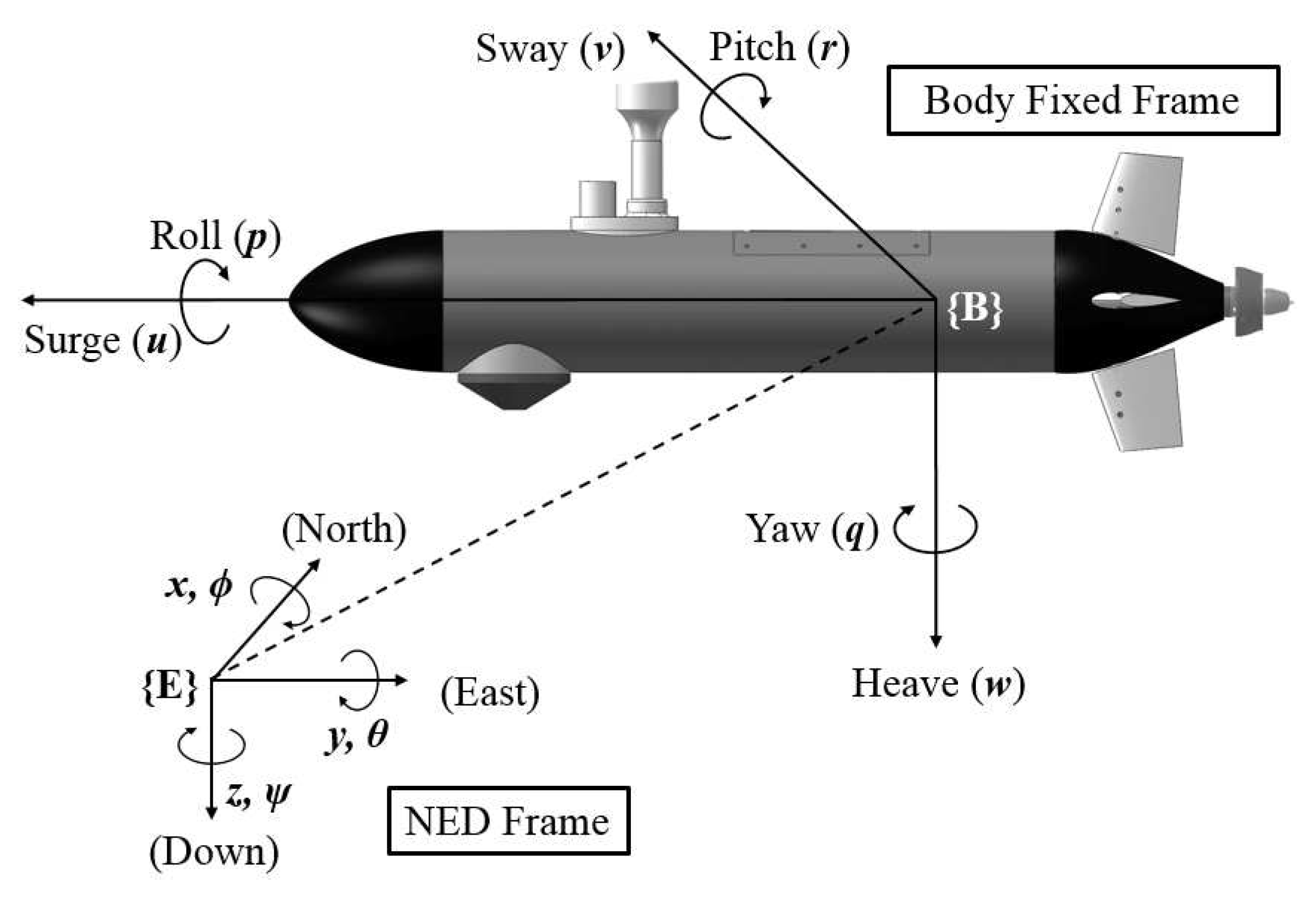
2. Problem Formulation in 3D Plane

This section deals with the formulation of the control problem using the AURV model. The AURV model is reduced and presented in terms of two subsystems in the vertical as well as horizontal plane. The states involved in a vertical plane include surge, heave, and pitch motion. On the other hand, the horizontal plane includes the state’s surge, sway, and yaw. Modeling of AURV in a 3D plane is explained by the kinematics and dynamics involved in the vertical plane and horizontal plane simultaneously.

Table 1. Nomenclature.

Symbols	Description
F	Body fixed frame
O	NED frame
T	Serret-Frenet reference frame
m	Mass of the AURV
W	Weight of AURV
B	Buoyancy Force
$u,v,w,q,r$	Linear and angular velocities
$x,y,z,\theta ,\psi$	Linear and angular positions
$I_x,I_y,I_z$	Moments of inertia about x, y, and z axes in the body-fixed frame
($x_B,y_B,z_B$)	Center of buoyancy
($x_G,y_G,z_G$)	Center of gravity
T	Total thrust in vertical plane and horizontal plane
($\mathrm{\Xi },ϵ$)	Lyapunov function
${\delta }_s$	Stern angle
${\delta }_r$	Rudder angle
{$x_{f/t}$}	Error Space between body and SF frame along X-Axis
{$y_{f/t}$}	Error Space between body and SF frame along Y-Axis
$d_{TO}$	Position of T frame relative to O frame
$d_{FT}$	Position of F frame relative to T frame
$d_{FO}$	Position of F frame relative to O frame
$c_a$	Curvilinear abscissa along the path
${\psi }_t$	Yaw angle between O and T coordinate system
Subscripts
d	Parameters of vertical plane
h	Parameters of horizontal plane
D	Desired values for depth tracking and yaw tracking
t	Parameters of Serret-Frenet frame
E	Error representation for depth and yaw

indicates the various notations used to represent the dynamics and kinematics of the system. Figure 1 shows the schematic diagram of AURV with different motions concerning the body and earth frames. Similarly, Figure 2 presents the different planes of an AURV. The AURV is modeled in a 3D plane under the following assumptions.

Assumption 1. 

A constant surge velocity is maintained through the analysis of 3D control algorithm.

Remark 1. 

The design of the control algorithm deals with the path following control for which the time factor is not a crucial one.

Assumption 2. 

The roll motion of AURV is neglected.

Remark 2. 

The roll effect is significant during the 3D motion of an AURV wherein diving and steering dynamics are coupled. Here, the controller is designed for the diving and heading control separately where the effect of roll motion is not significant. Furthermore, an Infante flat-fish type of AURV has been considered in this paper for which roll motion is not desirable.

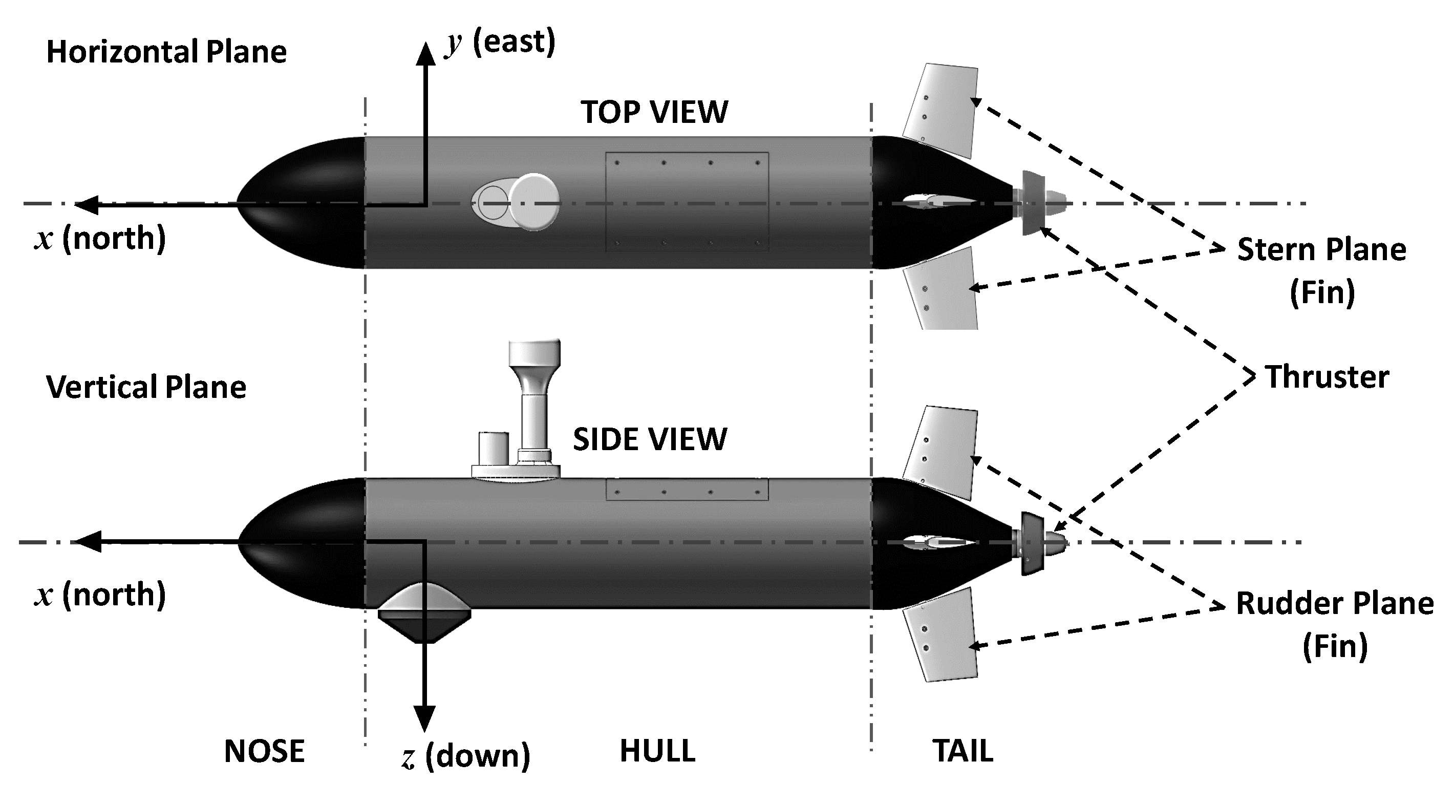
2.1. AURV Modeling in Vertical Plane

The Kinematics of AURV in vertical plane is given by

$$\begin{array}{ccc}\hfill {\stackrel{{\displaystyle \blacksquare }}{x}}_d& =& u_{d}cos{\theta }_d+w_{d}sin{\theta }_d\hfill \end{array}$$

(1)

$$\begin{array}{ccc}\hfill {\stackrel{{\displaystyle \blacksquare }}{z}}_d& =& -u_{d}sin{\theta }_d+w_{d}cos{\theta }_d\hfill \end{array}$$

(2)

$$\begin{array}{ccc}\hfill {\stackrel{{\displaystyle \blacksquare }}{\theta }}_d& =& q{}_d\hfill \end{array}$$

(3)

The AURV dynamics is given as

$$\begin{array}{ccc}\hfill m{\stackrel{{\displaystyle \blacksquare }}{u}}_d& =& C_{X_{uu}}{u}_d^2+C_{X_{ww}}w{}_d^2+C_{X{}_{qq}}{q}_d^2+u_d^2{C}_{X_{\delta s\delta s}}{\delta }_s^2+C_{X_u^{{\displaystyle \blacksquare }}}{\stackrel{{\displaystyle \blacksquare }}{u}}_d+T_d\hfill \end{array}$$

(4)

$$\begin{array}{ccc}\hfill ({\stackrel{{\displaystyle \blacksquare }}{w}}_d-u_d{q}_d)& =& (W-B)cos{\theta }_d+C_{Z_w}{u}_d{w}_d+C_{Z_q}{u}_d{q}_d+C_{Z_{\delta s}}{u}_{d^2}{\delta }_s+C_{Z_w^{{\displaystyle \blacksquare }}}{\stackrel{{\displaystyle \blacksquare }}{w}}_d\hfill \end{array}$$

(5)

$$\begin{array}{ccc}\hfill I_y{\stackrel{{\displaystyle \blacksquare }}{q}}_d& =& z_{B}Bsin{\theta }_d+C_{M_w}{u}_d{w}_d+C_{M_q}{u}_d{q}_d+C_{M_{\delta s}}{u}_d^2{\delta }_s+C_{M_q^{{\displaystyle \blacksquare }}}{\stackrel{{\displaystyle \blacksquare }}{q}}_d\hfill \end{array}$$

(6)

A constant forward velocity is considered to describe the nonlinear structure of AURV which is expressed as

$$\begin{array}{c}\hfill \dot{x}=f_{xd}\left(x\right)+g_{xd}\left(u\right)\end{array}$$

(7)

where,

$$\begin{array}{cc}\hfill f_{xd}=& \left[\begin{array}{c}((W-B)cos\left({\theta }_d\right)+\left(C_{z_w}{u}_d{w}_d\right)\\ +(C_{z_q}{u}_d{q}_d+\left(m{u}_d{q}_d\right))/(m-C_{z_{\dot{w}}})\\ (Z_{B}Bsin{\theta }_d+\left(C_{M_w}{u}_d{w}_d\right)\\ +\left(C_{M_q}{u}_d{q}_d\right))/(I_y-C_{M_{\dot{q}}})\\ q_d\end{array}\right]\end{array}$$

(8)

$$\begin{array}{cc}\hfill g_{xd}=& \left[\begin{array}{c}\frac{\left(C_Z{\delta }_s{u}_{d^2}\right)}{(m-C_{Z_{\dot{W}}})}\\ \frac{\left(C_m{\delta }_s{u}_{d^2}\right)}{I_y-C_{m_{\dot{q}}}}\\ 0\end{array}\right]\end{array}$$

(9)

where $x=[w_d,q_d,{\theta }_d]$ and $u={\delta }_s$.

2.2. AURV Modeling in Horizontal Plane

The kinematics of AURV in horizontal plane is given by

$$\begin{array}{ccc}\hfill {\dot{x}}_h& =& u_{h}cos\left({\psi }_h\right)-v_{h}sin\left({\psi }_h\right)\hfill \end{array}$$

(10)

$$\begin{array}{ccc}\hfill {\dot{y}}_h& =& -u_{h}sin\left({\psi }_h\right)+v_{h}cos\left({\psi }_h\right)\hfill \end{array}$$

(11)

$$\begin{array}{ccc}\hfill {\dot{\psi }}_h& =& r_h\hfill \end{array}$$

(12)

Subsequently, the AURV dynamics is given as

$$\begin{array}{ccc}\hfill m{\dot{u}}_h& =& C_{X_{uu}}{u}_h^2+C_{X_{vv}}{v}_h^2+C_{X_{rr}}{r}_h^2+u_h^2{C}_{X_{{\delta }_r{\delta }_r}}{\delta }_r^2+C_{X_{\dot{u}}}{\dot{u}}_h+T_h\hfill \end{array}$$

(13)

$$\begin{array}{ccc}\hfill m({\dot{v}}_h+u_h{r}_h)& =& C_{Y_{\delta r}}{u}_h^2{\delta }_r+C_{Y_r}{u}_h{r}_h+C_{Y_v}{u}_h{v}_h+C_{Y_{\dot{v}}}{\dot{v}}_h+C_{Y_{r\left|r\right|}}{r}_h\left|r_h\right|+C_{Y_{v\left|v\right|}}{v}_h\left|v_h\right|\hfill \end{array}$$

(14)

$$\begin{array}{ccc}\hfill I_z{\dot{r}}_h& =& C_{N_v}{u}_h{v}_h+C_{N_r}{u}_h{r}_h+C_{N_{r\left|r\right|}}{r}_h\left|r_h\right|+C_{N_{v\left|v\right|}}{v}_h\left|v_h\right|+C_{N_r^{{\displaystyle \blacksquare }}}{\dot{r}}_h+C_{N_{\delta r}}{u}_h^2{\delta }_h\hfill \end{array}$$

(15)

where, the hydrodynamics coefficients $\left[C_{(·)}\right]$ are considered from the article [42,43]. Similarly, the nonlinear structure of AURV in the horizontal plane is expressed as

$$\dot{x}=f_{xh}\left(x\right)+g_{xh}\left(x\right)u$$

(16)

where $x=[v_h,r_h,{\psi }_h]$ and $u={\delta }_r$ and

$$\begin{array}{c}\hfill f_{xh}\left(x\right)=\left(\begin{array}{c}(C_{Y_{r\left|r\right|}}{r}_h\left|r_h\right|+C_{Y_{v\left|v\right|}}{v}_h\left|v_h\right|+C_{Y_r}{u}_h{r}_h\\ +C_{Y_v}{u}_h{v}_h-m{u}_h{r}_h)/(m-C_{Y_{\dot{v}}})\\ (C_{N_v}{u}_h{v}_h+C_{N_r}{u}_h{r}_h+C_{N_{r\left|r\right|}}{r}_h\left|r_h\right|\\ +C_{N_{v\left|v\right|}}{v}_h\left|v_h\right|)/(I_z-C_{N_{\dot{r}}})\\ r_h\\ \end{array}\right)\end{array}$$

(17)

$$\begin{array}{c}\hfill g_{xh}\left(x\right)=\left[\begin{array}{c}\left(C_{Y_{\delta r}}{u}_h^2\right)/(m-C_{Y_{\dot{v}}})\\ \left(C_{N_{\delta r}}{u}_h^2\right)/(I_z-C_{N_{\dot{r}}})\\ 0\end{array}\right]\end{array}$$

(18)

The design of the control algorithm is carried out for a decoupled model of diving and steering planes. However, a 3D path following task is achieved by considering the combination of both as described in Figure 3. Besides, the path following task is achieved by considering the kinematic model for AURV in terms of the SF frame.

A generalized linear system is considered as shown below by linearizing the nonlinear AURV model as described earlier to the design of the control algorithm.

$$\begin{array}{c}\hfill \begin{array}{cc}\hfill \dot{x}& ={\mathcal{H}}_{T}x+{\mathcal{G}}_{T}u\hfill \\ \hfill y& ={\mathfrak{C}}_{T}x\hfill \end{array}\end{array}$$

(19)

where ${\mathcal{H}}_T\in {\mathcal{R}}^{n\mathrm{x}n}$, ${\mathcal{G}}_T\in {\mathcal{R}}^{n\mathrm{x}m}$, ${\mathfrak{C}}_T\in {\mathcal{R}}^{r\mathrm{x}n}$ are the state matrix, input matrix, and output matrix respectively.

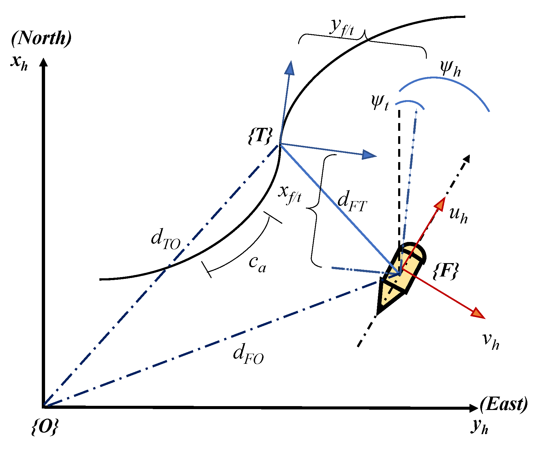
2.3. Path Following Kinematics: Serret-Frenet Frame

The S-F frame is used in designing a kinematic model for the AURV so that the 3D path following task of an AURV is achieved. In achieving a path following task, the time factor is not considered a constraint. The objective is that AURV needs to be converged along the specified path placed at some depth by considering the SF frame as shown in Figure 4. The kinematic model in terms of SF frame is represented as follows

$$\begin{array}{ccc}\hfill \left(\begin{array}{c}{\dot{x}}_{f/t}\\ {\dot{y}}_{f/t}\end{array}\right)& =& \left(\begin{array}{cc}cos{\psi }_{tf}& -sin{\psi }_{tf}\\ sin{\psi }_{tf}& cos{\psi }_{tf}\end{array}\right)-\left(\begin{array}{c}{\dot{c}}_a\\ 0\end{array}\right)-{\dot{c}}_a\left(\begin{array}{cc}0& -p_e\left(c_a\right)\\ p_e\left(c_a\right)& 0\end{array}\right)\left(\begin{array}{c}{x}_{f/t}\\ y_{f/t}\end{array}\right)\hfill \end{array}$$

(20)

where ${\psi }_{tf}$ = ${\psi }_t-{\psi }_f$, denotes the steering angle of the body relative to the steering angle of SF, $p_e\left(c_a\right)$ indicates the path curvature for a circular path and ${\left(x_{f/t},y_{f/t}\right)}^T$ indicate the error space between body and SF frame along X and Y axes respectively.

2.4. Problem Statement

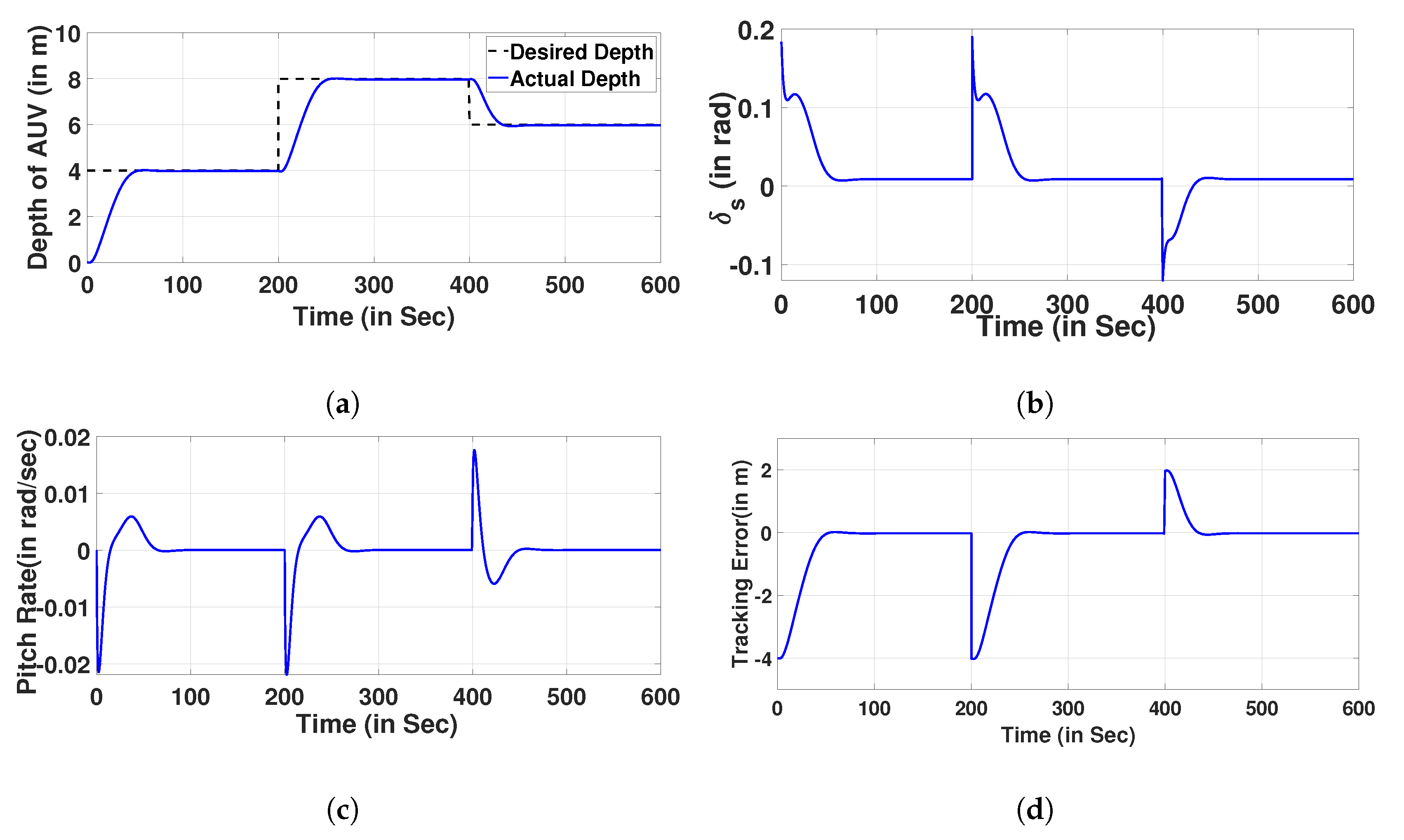
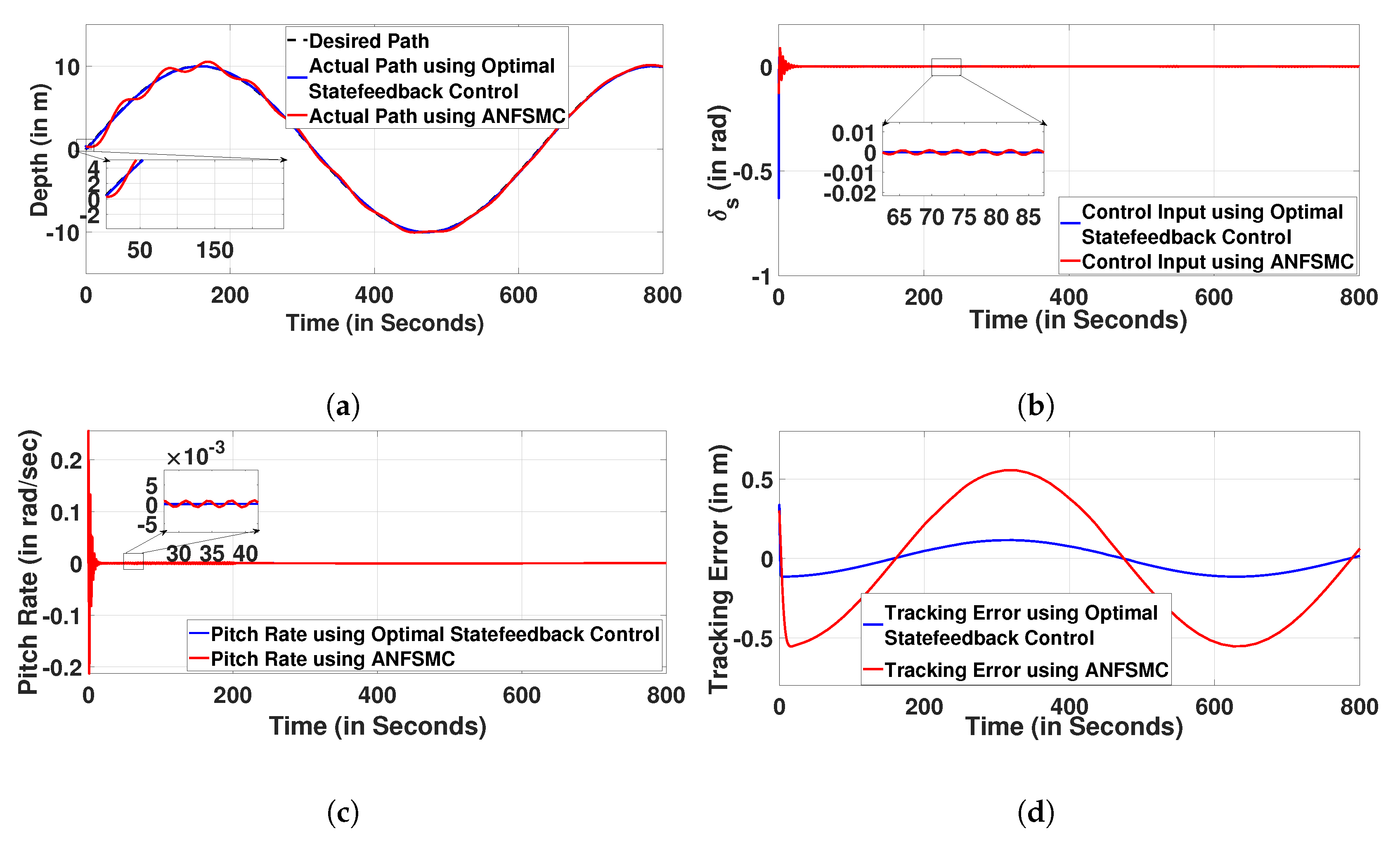
In the design of a 3D path following control algorithm, the desired depth and desired yaw need to be achieved by minimizing the depth error and yaw orientation error respectively. Furthermore, the path following task needs to be achieved through the guidance law. The state feedback optimal control algorithm is developed using Equation (19).

• The desired depth $z_D$ is achieved by minimizing the depth error, i.e.,

  $$\underset{t\to 0}{lim}{z}_E\left(t\right)=0$$

  (21)

  where $z_E=z_d-z_D$. It is intended to design a backstepping control algorithm to achieve an Equation (21).
• Subsequently, a desired pitch angle ${\theta }_D$ is achieved by reducing the pitch orientation error to zero, i.e.,

  $$\underset{t\to 0}{lim}{\theta }_E\left(t\right)=0$$

  (22)

  where ${\theta }_E={\theta }_d-{\theta }_D$. As a cascaded structure is adopted in the control structure, the desired pitch angle is generated by the backstepping approach. In this, an optimal robust control strategy is designed to achieve the Equation (22).
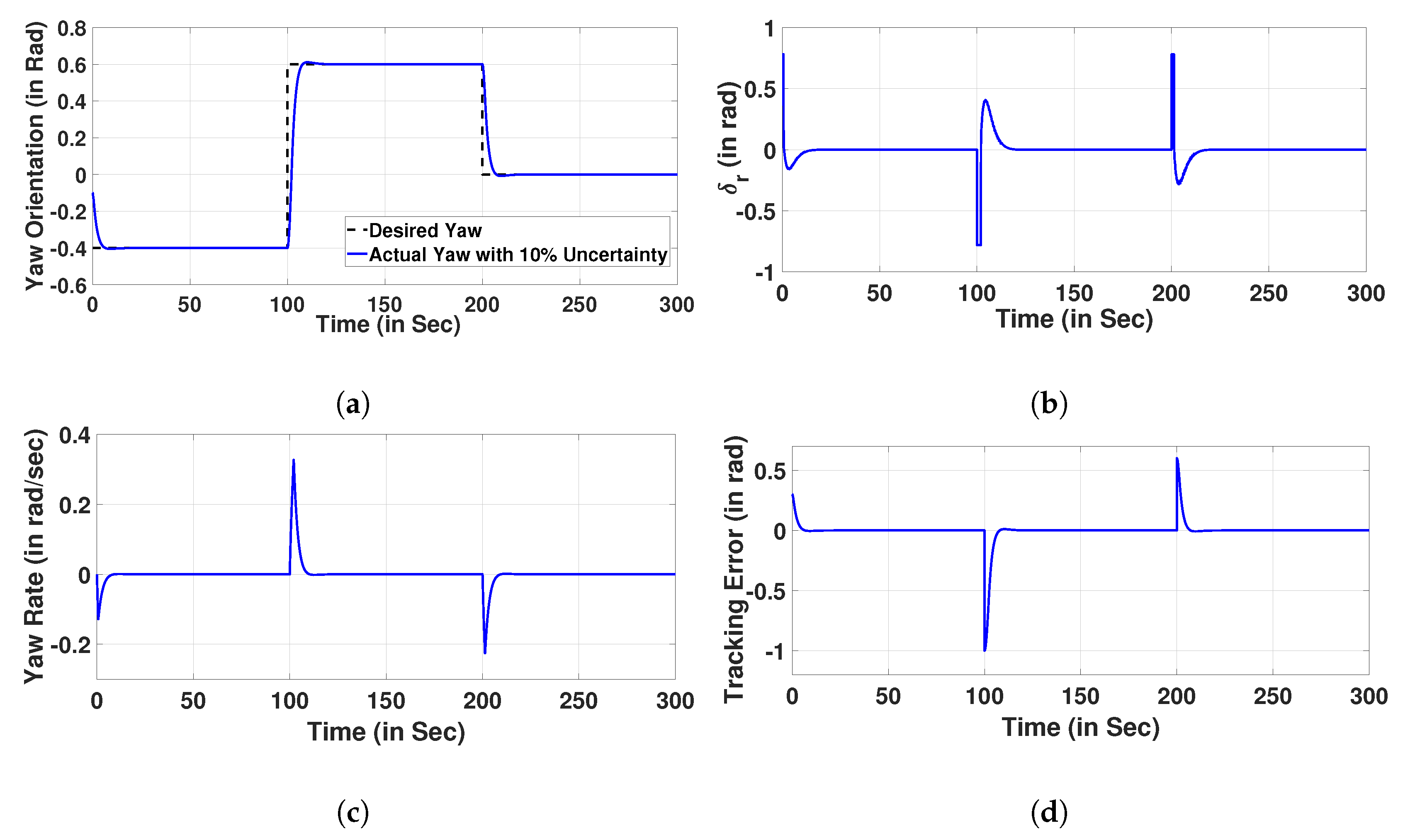
• The desired yaw ${\psi }_h$ needs to be achieved by minimizing the yaw error i.e.,

  $$\underset{t\to 0}{lim}{\psi }_E\left(t\right)=0$$

  (23)

  where ${\psi }_E={\psi }_h-{\psi }_D$. The design of the backstepping controller is intentionally made to achieve an Equation (23).
• Subsequently, yaw orientation error is reduced to zero to achieve the desired yaw angle ${\psi }_D$ i.e.,

  $$\underset{t\to 0}{lim}{r}_E\left(t\right)=0$$

  (24)

  where $r_E=r_h-r_D$. A cascaded structure is adapted in the control design and the backstepping approach is employed in producing the desired yaw angle.

3. Control of AURV Kinematics

This section explores the control of the kinematics of the AURV system through the backstepping approach in both the vertical plane and the horizontal plane. Furthermore, an explanation of the guidance law required for the path following through the SF frame is also exploited.

3.1. Backstepping Approach for Depth Control

The desired depth of AURV is tracked efficiently by employing the backstepping technique. The backstepping technique requires the desired pitch angle which is obtained through the following theorem. This pitch angle is further used in the proposed robust state feedback optimal control law. Figure 3 depicts the backstepping approach involved in the vertical plane.

Theorem 1. 

Considering the Equation (2) a desired pitch angle is derived as follows

$$\begin{array}{c}\hfill {\theta }_D={\theta }_{G}tanh\left({\mathcal{K}}_p{z}_e\right)+{\sigma }_G\end{array}$$

(25)

where ${\theta }_G$ indicates the maximum allowable approaching angle, ${\mathcal{K}}_p$ is a positive gain and ${\sigma }_G$ = ${tan}^{-1}(w_d/u_d)$.

Proof. 

The existence of Lyapunov function ${\mathrm{\Xi }}_d=1/2\left({z_e}^2\right)$ is shown for all values of $z_e$ provided, ${\mathrm{\Xi }}_d\le 0$ Derivation of the Lyapunov function will further lead to

$$\begin{array}{c}\hfill {\dot{\mathrm{\Xi }}}_d=z_e{\dot{z}}_d=-u_d{z}_{e}sin{\theta }_d+w_d{z}_{e}cos{\theta }_d\end{array}$$

(26)

Furthermore the above Equation (26) is simplified as shown below.

$$\begin{array}{ccc}\hfill {\dot{\mathrm{\Xi }}}_d& =& -w_v(sin{\theta }_{d}cos{\sigma }_G-cos{\theta }_{d}sin{\sigma }_G)\hfill \end{array}$$

(27)

$$\begin{array}{ccc}\hfill {\dot{\mathrm{\Xi }}}_d& =& -w_{v}sin({\theta }_d-{\sigma }_G)\hfill \end{array}$$

(28)

where $w_v=\sqrt{{u_d}^2+{w_d}^2}$. Hence, for ${\theta }_d-{\sigma }_G={\theta }_{G}tanh\left({\mathcal{K}}_p{z}_e\right)$ the condition ${\dot{\mathrm{\Xi }}}_d\le 0$ will always be satisfied irrespective of $z_e$ value. □

3.2. Backstepping Approach for Yaw Control

Here, the backstepping approach in the horizontal plane is discussed for effective yaw tracking. The backstepping approach is used in the generation of a desired yaw orientation. Furthermore, the same backstepping law is applied to generate the desired yaw angle. Figure 3 depicts the backstepping approach involved in a horizontal plane.

Theorem 2. 

A desired yaw rate is derived by referring to Equation (12).

$$\begin{array}{c}\hfill r_D=-{\mathcal{K}}_{\psi h}{\psi }_E\end{array}$$

(29)

where ${\mathcal{K}}_{\psi h}$ indicates the positive gain and ${\psi }_E$ represent the yaw tracking error.

Proof. 

The existence of a Lyapunov function ${\epsilon }_h=\frac{1}{2}{\psi }_E^2$ is shown for all values of ${\psi }_E$ such that ${\epsilon }_h\le 0$. The further computation of the derivative of the Lyapunov function is given as

$$\begin{array}{ccc}\hfill \dot{{\epsilon }_h}& =& {\psi }_E{\dot{\psi }}_E\hfill \end{array}$$

(30)

$$\begin{array}{ccc}\hfill {\psi }_E& =& {\psi }_h-{\psi }_D\hfill \end{array}$$

(31)

On computing the derivative of (31),

$$\begin{array}{ccc}\hfill {\dot{\psi }}_E& =\hfill & \hfill r_h\end{array}$$

(32)

From (30) and (32), it is obtained as

$$\dot{{\epsilon }_h}={\psi }_E\left(r_h\right)$$

(33)

Considering $r_h$ as $r_D$ it is desired to get $\dot{{\epsilon }_h}=-{\mathcal{K}}_{\psi h}{\psi }_E$ the condition $\dot{{\epsilon }_h}\le 0$ will always be satisfied irrespective of any value of ${\psi }_E$. □

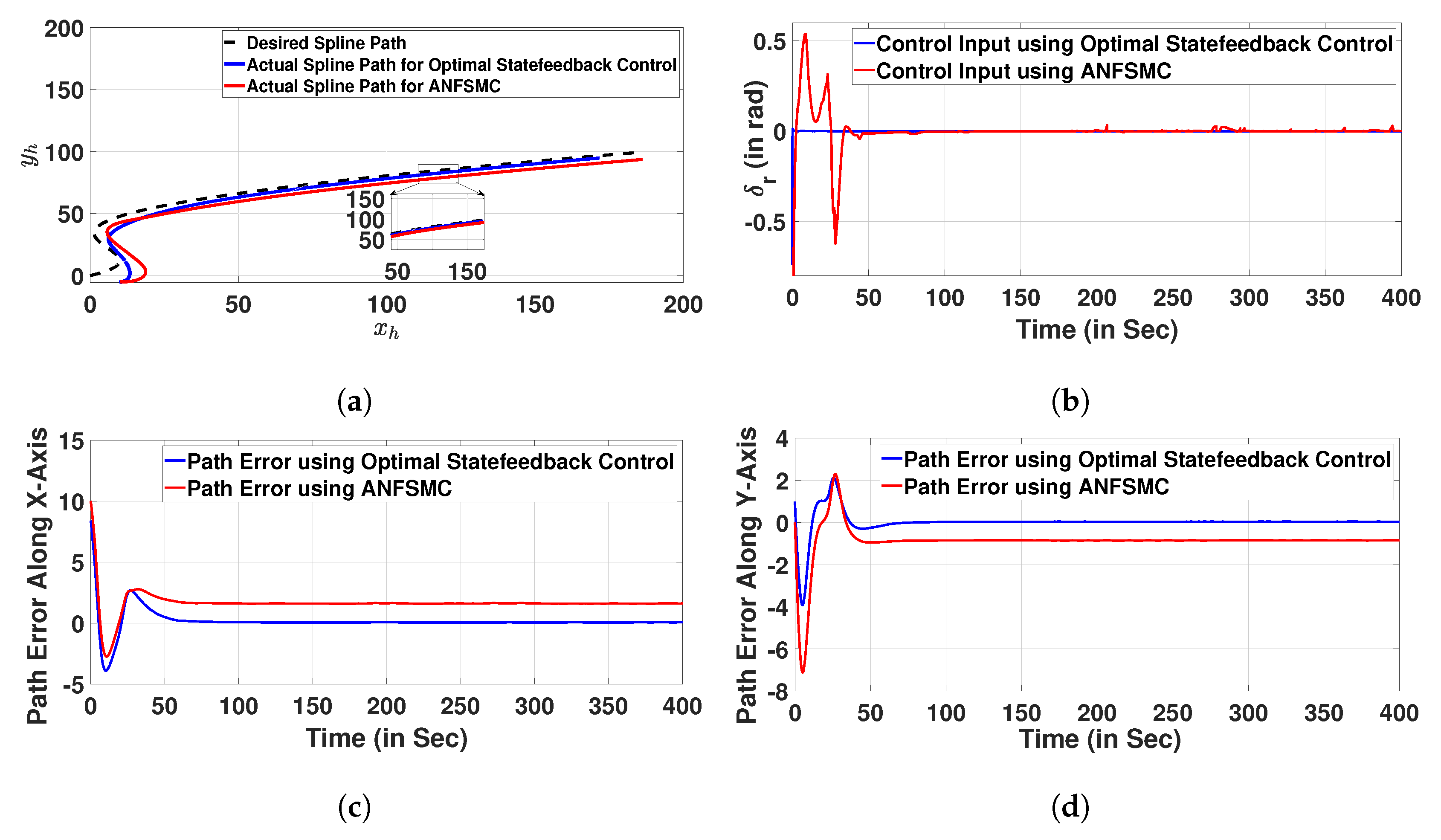
3.3. Path Following Guidance Law

Guidance law is presented in this section which considers the SF frame so that the path following task can be achieved. Besides, a desired yaw which is generated by the guidance law is tracked as shown in Figure 3. Figure 3 indicates the control strategy associated with the path following. Furthermore, guidance law is employed to obtain an appropriate desired yaw angle for the AURV to converge into the path. The error coordinates of the body and SF frames have to be minimized. They are described as follows

$$\underset{t\to \infty }{lim}{x}_{f/t}=0,\underset{t\to \infty }{lim}{y}_{f/t}=0$$

(34)

For the path following problem to be realized, it requires the guidance and update law [10] which are given as

$$\begin{array}{ccc}\hfill {\psi }_D& =& {\psi }_t-{tan}^{-1}\left[\frac{v_h}{u_h}\right]-{tan}^{-1}\left[\frac{y_{f/t}}{\sqrt{{{\chi }_{3D}}^2+{\left(x_{f/t}\right)}^2}}\right]\hfill \end{array}$$

(35)

$$\begin{array}{ccc}\hfill {\dot{c}}_a& =& \sqrt{{u_h}^2+{v_h}^2}\left[\frac{\sqrt{{{\chi }_{3D}}^2+{\left(x_{f/t}\right)}^2}+x_{f/t}}{\sqrt{{{\chi }_{3D}}^2+{\left(x_{f/t}\right)}^2+{\left(y_{f/t}\right)}^2}}\right]\hfill \end{array}$$

(36)

where ${\chi }_{3D}$ indicates a positive design parameter known as look-ahead distance. It is treated as a constant, function of time, error coordinates, or any other parameters. In this case, it is appropriated as a constant.

4. Control of AURV Dynamics

Referring to Figure 3, this section exploits the robust optimal control algorithm in the diving plane and steering plane. Here, stability analysis in terms of LMI and robustness is explored.

4.1. LMI Based Optimal State Feedback Controller

The linearized AURV system represented by Equation (19) is controlled by describing the LMI-based control algorithm.

Lemma 1. 

For the closed loop system to be asymptotically stable, a constant gain matrix ${\mathcal{K}}_T\in {\mathbb{R}}^{nxn}$ such that

$$u=-{\mathcal{K}}_{T}x$$

(37)

Proposition 1. 

Referring to linearized system (19) and Equation (37), the closed loop system is represented as

$$\dot{x}=({\mathcal{H}}_T-{\mathcal{G}}_T{\mathcal{K}}_T)x$$

(38)

This proposition will have a solution which is described in the next theorem.

Theorem 3. 

If the matrices $\mathcal{P}$ and $\mathcal{R}$ exist, then the solution to proposition 1 exists whose necessary and sufficient condition will depend on the matrices where $\mathcal{P}={\mathcal{P}}^T$, $\mathcal{P}\in {\mathbb{R}}^{nxn}$, $R\in {\mathbb{R}}^{nxn}$ such that

$$\begin{array}{c}\hfill \begin{array}{c}\hfill -{{\mathcal{H}}_T}^T\mathcal{P}-\mathcal{P}{\mathcal{H}}_T+\mathcal{P}{\mathcal{G}}_T({\mathcal{R}}^{-T}+{\mathcal{R}}^{-1}){{\mathcal{G}}_T}^T\mathcal{P}\le 0\\ \hfill \mathcal{P}\ge 0\end{array}\end{array}$$

(39)

On satisfying the above condition (39), a state feedback matrix that solves Proposition 1 is given by

$$\begin{array}{c}\hfill {\mathcal{K}}_T={\mathcal{R}}^{-1}{{\mathcal{G}}_T}^T\mathcal{P}\end{array}$$

(40)

Proof. 

Taking ${\mathcal{V}}_{\mathcal{T}}\left(x\right)=x^T\mathcal{P}x$, where $\mathcal{P}$ is a positive definite matrix, i.e., $\mathcal{P}>0$, the closed loop system stability is discussed. For the closed loop system (38) to be stable, the condition that has to be satisfied is that the energy should decrease with time i.e., ${\dot{\mathcal{V}}}_T\le 0$. Then, ${\dot{\mathcal{V}}}_T$ is presented as

$$\begin{array}{c}\hfill {\dot{\mathcal{V}}}_T\left(x\right)={\dot{x}}^T\mathcal{P}x+x^T\mathcal{P}\dot{x}\end{array}$$

(41)

From Equations (19) and (37)

$$\begin{array}{cc}\hfill {\dot{\mathcal{V}}}_T\left(x\right)& ={\left[({\mathcal{H}}_T-{\mathcal{G}}_T{\mathcal{K}}_T)x\right]}^T\mathcal{P}x+x^T\mathcal{P}\left[({\mathcal{H}}_T-{\mathcal{G}}_T{\mathcal{K}}_T)x\right]\hfill \end{array}$$

(42)

From Equation (40), the above expression is represented as

$$\begin{array}{}\mathrm{(43)}& \hfill {\dot{\mathcal{V}}}_T\left(x\right)& =& x^T[({{\mathcal{H}}_T}^T-{\left({\mathcal{R}}^{-1}{{\mathcal{G}}_T}^T\mathcal{P}\right)}^T{{\mathcal{G}}_T}^T)\mathcal{P}+\mathcal{P}({\mathcal{H}}_T-{\mathcal{G}}_T\left({\mathcal{R}}^{-1}{{\mathcal{G}}_T}^T\mathcal{P}\right)]x\hfill \mathrm{(44)}& & =& x^T\left[({{\mathcal{H}}_T}^T\mathcal{P}+\mathcal{P}{\mathcal{H}}_T-\mathcal{P}{\mathcal{G}}_T{\mathcal{R}}^{-T}{{\mathcal{G}}_T}^T\mathcal{P}-\mathcal{P}{\mathcal{G}}_T{\mathcal{R}}^{-1}{{\mathcal{G}}_T}^T\mathcal{P})\right]x\hfill \end{array}$$

Rearranging the above equation, we get

$$\begin{array}{}\mathrm{(45)}& \hfill {\dot{\mathcal{V}}}_T\left(x\right)& =& -x^T[\mathcal{P}{\mathcal{G}}_T({\mathcal{R}}^{-T}+{\mathcal{R}}^{-1}){{\mathcal{G}}_T}^T\mathcal{P}-{{\mathcal{H}}_T}^T\mathcal{P}-\mathcal{P}{\mathcal{H}}_T]x\hfill \mathrm{(46)}& & =& -x^T[\mathcal{P}{\mathcal{G}}_T{\left({({\mathcal{R}}^{-T}+{\mathcal{R}}^{-1})}^{-1}\right)}^{-1}{{\mathcal{G}}_T}^T\mathcal{P}-{{\mathcal{H}}_T}^T\mathcal{P}-\mathcal{P}{\mathcal{H}}_T]x\hfill \mathrm{(47)}& & =& -x^T[\mathcal{P}{\mathcal{G}}_T{\left(Y\right)}^{-1}{{\mathcal{G}}_T}^T\mathcal{P}-{{\mathcal{H}}_T}^T\mathcal{P}-\mathcal{P}{\mathcal{H}}_T]x\hfill \end{array}$$

where $Y={({\mathcal{R}}^{-T}+{\mathcal{R}}^{-1})}^{-1}$ □

4.2. Robust LMI BASED Optimal Control Law

Referring to state space representation presented in Equation (19), the convex combination of polytope vertices is represented as

$$\begin{array}{c}\hfill \dot{x}\left(t\right)=\sum _{i=1}^n{\gamma }_i({{\mathcal{H}}_{TR}}_{i}x+{{\mathcal{G}}_{TR}}_{i}u)={\mathcal{H}}_{TR}\left(\gamma \right)x+{\mathcal{G}}_{TR}\left(\gamma \right)u\end{array}$$

(48)

where n represents the polytope vertices. The parameters ${\gamma }_i$, i = 1, 2, … n are considered as constant and real numbers of unknown type. They belong to unitary simplex $U_s$ which is given by

$$\begin{array}{ccc}\hfill U_s& =\hfill & \hfill \sum _{i=1}^n{\gamma }_i=1,{\gamma }_i\ge 0,i=1,2,\dots n\end{array}$$

(49)

Lemma 2. 

For the closed loop system to be asymptotically stable, a constant gain matrix ${\mathcal{K}}_{TR}\in {\mathbb{R}}^{nxn}$ such that

$$u=-{\mathcal{K}}_{TR}x$$

(50)

Proposition 2. 

Referring to (48) and (50), the closed loop system is expressed as

$$\begin{array}{c}\hfill \begin{array}{cc}\hfill \dot{x}& ={\mathcal{H}}_{TR}\left(\gamma \right)x+{\mathcal{G}}_{TR}\left(\gamma \right)(-{\mathcal{K}}_{TR}x)\hfill \\ \hfill \dot{x}& =({\mathcal{H}}_{TR}\left(\gamma \right)-{\mathcal{G}}_{TR}\left(\gamma \right){\mathcal{K}}_{TR})x\hfill \end{array}\end{array}$$

(51)

The following theorem will describe the solution for the above proposition.

Theorem 4. 

The solution to the Proposition 2 exists such that the necessary and sufficient conditions depend on the existence of matrices $\mathcal{P}={\mathcal{P}}^T$ and $\mathcal{R}$ where $\mathcal{P}\in {\mathcal{R}}^{nxn}$, $\mathcal{R}\in {\mathcal{R}}^{nxn}$ such that

$$\begin{array}{c}\hfill \begin{array}{c}\hfill -{{\mathcal{H}}_{TR}\left(\gamma \right)}^T\mathcal{P}-\mathcal{P}{\mathcal{H}}_{TR}\left(\gamma \right)+\mathcal{P}{\mathcal{G}}_{TR}\left(\gamma \right)({\mathcal{R}}^{-T}+{\mathcal{R}}^{-1}){{\mathcal{G}}_{TR}\left(\gamma \right)}^T\mathcal{P}\le 0.\\ \hfill \mathcal{P}\ge 0\end{array}\end{array}$$

(52)

When (52) is satisfied then a state feedback matrix that solves the Proposition 2 is given by

$$\begin{array}{c}\hfill {\mathcal{K}}_{TR}={\mathcal{R}}^{-1}{{\mathcal{G}}_{\mathcal{TR}}}^T\mathcal{P}\end{array}$$

(53)

Proof. 

Taking ${\mathcal{V}}_{\mathcal{TR}}\left(x\right)=x^T\mathcal{P}x$, i.e., $\mathcal{P}>0$, the closed loop system stability is discussed. For the closed loop system (38) to be stable, the condition that has to be satisfied is that the energy should decrease with time i.e., ${\dot{\mathcal{V}}}_{TR}\le 0$. Then, ${\dot{\mathcal{V}}}_{TR}$ is presented as

$$\begin{array}{c}\hfill {\dot{\mathcal{V}}}_{TR}\left(x\right)={\dot{x}}^T\mathcal{P}x+x^T\mathcal{P}\dot{x}\end{array}$$

(54)

From Equations (19) and (50)

$$\begin{array}{c}\hfill {\dot{\mathcal{V}}}_{TR}\left(x\right)={\left[({\mathcal{H}}_{TR}\left(\gamma \right)-{\mathcal{G}}_{TR}\left(\gamma \right){\mathcal{K}}_{TR})x\right]}^T\mathcal{P}x+x^T\mathcal{P}\left[({\mathcal{H}}_{TR}\left(\gamma \right)-{\mathcal{G}}_{TR}\left(\gamma \right){\mathcal{K}}_{TR})x\right]\end{array}$$

(55)

From Equation (53), the above expression is represented as

$$\begin{array}{ccc}\mathrm{(56)}& \hfill {\dot{\mathcal{V}}}_{TR}\left(x\right)& =& x^T[({\mathcal{H}}_{TR}{\left(\gamma \right)}^T-{\left({\mathcal{R}}^{-1}({\mathcal{G}}_{TR}{\left(\gamma \right))}^T\mathcal{P}\right)}^T({\mathcal{G}}_{TR}{\left(\gamma \right))}^T)\mathcal{P}\hfill \hfill & & +\mathcal{P}({\mathcal{H}}_{TR}\left(\gamma \right)-{\mathcal{G}}_T\left({\mathcal{R}}^{-1}({\mathcal{G}}_{TR}{\left(\gamma \right))}^T\mathcal{P}\right)]x\hfill \\ \mathrm{(57)}& & =& x^T\left[\right(({\mathcal{H}}_{TR}{\left(\gamma \right))}^T\mathcal{P}+\mathcal{P}{\mathcal{H}}_{TR}\left(\gamma \right)-\mathcal{P}{\mathcal{G}}_{TR}\left(\gamma \right){\mathcal{R}}^{-T}({\mathcal{G}}_{TR}{\left(\gamma \right))}^T\mathcal{P}\hfill \hfill & & -\mathcal{P}{\mathcal{G}}_{TR}\left(\gamma \right){\mathcal{R}}^{-1}({\mathcal{G}}_{TR}{\left(\gamma \right))}^T\mathcal{P}\left)\right]x\hfill \end{array}$$

Rearranging the above equation, we get

$$\begin{array}{ccc}\mathrm{(58)}& \hfill {\dot{\mathcal{V}}}_{TR}\left(x\right)& =& -x^T[\mathcal{P}{\mathcal{G}}_{TR}\left(\gamma \right)({\mathcal{R}}^{-T}+{\mathcal{R}}^{-1})({\mathcal{G}}_{TR}{\left(\gamma \right))}^T\mathcal{P}\hfill \hfill & & -({\mathcal{H}}_{TR}{\left(\gamma \right))}^T\mathcal{P}-\mathcal{P}{\mathcal{H}}_{TR}\left(\gamma \right)]x\hfill \\ \mathrm{(59)}& & =& -x^T[\mathcal{P}{\mathcal{G}}_{TR}\left(\gamma \right){\left({({\mathcal{R}}^{-T}+{\mathcal{R}}^{-1})}^{-1}\right)}^{-1}({\mathcal{G}}_{TR}{\left(\gamma \right))}^T\mathcal{P}\hfill \hfill & & -({\mathcal{H}}_{TR}{\left(\gamma \right))}^T\mathcal{P}-\mathcal{P}{\mathcal{H}}_{TR}\left(\gamma \right)]x\hfill \\ \mathrm{(60)}& & =& -x^T[\mathcal{P}{\mathcal{G}}_{TR}\left(\gamma \right){\left(Y\right)}^{-1}({\mathcal{G}}_{TR}{\left(\gamma \right))}^T\mathcal{P}\hfill \hfill & & -({\mathcal{H}}_{TR}{\left(\gamma \right))}^T\mathcal{P}-\mathcal{P}{\mathcal{H}}_{TR}\left(\gamma \right)]x\hfill \end{array}$$

where $Y={({\mathcal{R}}^{-T}+{\mathcal{R}}^{-1})}^{-1}$

Furthermore, the above condition (52) is represented in LMI form as shown below.

$$\left(\begin{array}{cc}-{{\mathcal{H}}_{TR}\left(\gamma \right)}^T\mathcal{P}-\mathcal{P}{\mathcal{H}}_{TR}\left(\gamma \right)& -\mathcal{P}{\mathcal{G}}_{TR}\left(\gamma \right)\\ {{\mathcal{G}}_{TR}\left(\gamma \right)}^T\mathcal{P}& Y\end{array}\right)\le 0$$

(61)

Now for the system to be stable, ${\dot{\mathcal{V}}}_{TR}\le 0$, which indicates that $P{\mathcal{G}}_{TR}\left(\gamma \right){\left(Y^{-1}\right)}^{-1}{{\mathcal{G}}_{TR}\left(\gamma \right)}^T\mathcal{P}-({{\mathcal{H}}_{TR}\left(\gamma \right)}^T\mathcal{P}+\mathcal{P}{\mathcal{H}}_{TR}\left(\gamma \right))$ has to be positive definite. From the above, it is deduced that the condition (52) exists for the system (48) where ${\mathcal{H}}_{TR}\left(\gamma \right)$ = ${\gamma }_1\mathcal{H}{}_{{TR}_1}+{\gamma }_2\mathcal{H}{}_{{TR}_2}+\dots +{\gamma }_n\mathcal{H}{}_{{TR}_n}$ and ${\mathcal{G}}_{TR}\left(\gamma \right)$ = ${\gamma }_1\mathcal{G}{}_{T_1}+{\gamma }_2\mathcal{G}{}_{T_2}+\dots +{\gamma }_n\mathcal{G}{}_{T_n}$. Finally, concerning Theorem 4, the matrix $\mathcal{P}={\mathcal{P}}^T$ exists such that (52) holds which will be a sufficient condition for the solution of Proposition 2. Furthermore, the above condition (61) is represented by considering the polytopic vertices as

$$\left(\begin{array}{cc}-{\mathcal{H}{}_{{TR}_i}}^T\mathcal{P}-\mathcal{P}\mathcal{H}{}_{{TR}_i}& -\mathcal{P}\mathcal{G}{}_{{TR}_i}\\ {\mathcal{G}{}_{{TR}_i}}^T\mathcal{P}& Y\end{array}\right)\le 0$$

(62)

where $i=1,2,\dots n$, indicate the number of polytopic vertices. □

5. Results and Discussion

This section elaborates on the numerical analysis of the proposed control algorithm along with the simulation results. The simulation results and the numerical analysis are presented for both the vertical plane, the horizontal plane, and the 3D plane. The equilibrium point is considered as [0.1, 0.1, 0.1] and [0.1, 0.1] for the vertical plane and horizontal plane respectively. Referring to Section 2, the state matrix, input matrix, and output matrix are obtained by considering the equilibrium point as [$w_d$, $q_d$, ${\theta }_d$] = [0.1 0.1 0.1].

$${\mathcal{H}}_{\mathcal{T}}=\left(\begin{array}{ccc}-0.8761& 1.4166& -0.0003\\ 1.2450& -3.7164& -0.2633\\ 0& 1.000& 0\end{array}\right),$$

$${\mathcal{G}}_{\mathcal{T}}=\left(\begin{array}{c}-0.4027\\ -0.9331\\ 0\end{array}\right),{\mathcal{C}}_{\mathcal{T}}=\left(\begin{array}{ccc}0& 0& 1\end{array}\right)$$

The simulation of the developed control algorithm is carried out by considering a constant surge velocity of $u_d$ = 2 m/s. Considering the nonlinear AURV structure as shown in (7), the generation of polytopic vertices of AURV is considered for the uncertainty of $10\%$ change in the hydrodynamic parameters $C_{Z_{\dot{w}}}$ and $C_{M_{\dot{q}}}$. The ranges of the values to generate the polytope vertices for $10\%$ uncertainty are depicted in the

Table 2. Robustness Analysis Showing Different ranges of $C_{Z_{\dot{w}}}$ and $C_{M_{\dot{q}}}$ in vertical plane.

Hydrodynamic Parameters	Uncertainty Percentage	Range Obtained
$C_{Z_{\dot{w}}}$	$\pm 10\%$	$-5079.25$$\le C_{Z_{\dot{w}}}\le -4155.75$
$C_{M_{\dot{q}}}$	$\pm 10\%$	$-1861.64$$\le C_{M_{\dot{q}}}\le -1523.16$

.

For an uncertainty of $\pm 10\%$, the polytope vertices of AURV are generated as shown below.

$$\begin{array}{c}\hfill {\mathcal{H}}_{T1}=\left(\begin{array}{ccc}-0.8208& 1.3271& -0.0003\\ 1.3104& -3.9116& -0.2772\\ 0& 1.0000& 0\end{array}\right)\end{array}$$

$$\begin{array}{c}\hfill {\mathcal{H}}_{T2}=\left(\begin{array}{ccc}-0.8208& 1.3271& -0.0003\\ 1.1859& -3.5399& -0.2508\\ 0& 1.0000& 0\end{array}\right)\end{array}$$

$$\begin{array}{c}\hfill {\mathcal{H}}_{T3}=\left(\begin{array}{ccc}-0.9394& 1.5189& -0.0004\\ 1.3104& -3.9116& -0.2772\\ 0& 1.0000& 0\end{array}\right)\end{array}$$

$$\begin{array}{c}\hfill {\mathcal{H}}_{T4}=\left(\begin{array}{ccc}-0.9394& 1.5189& -0.0004\\ 1.1859& -3.5399& -0.2508\\ 0& 1.0000& 0\end{array}\right)\end{array}$$

and

$${\mathcal{G}}_{T1}=\left(\begin{array}{c}-0.3773\\ -0.9821\\ 0\end{array}\right),{\mathcal{G}}_{T2}=\left(\begin{array}{c}-0.3773\\ -0.8888\\ 0\end{array}\right)$$

$${\mathcal{G}}_{T3}=\left(\begin{array}{c}-0.4318\\ -0.9821\\ 0\end{array}\right),{\mathcal{G}}_{T4}=\left(\begin{array}{c}-0.4318\\ -0.8888\\ 0\end{array}\right)$$

Semi-definite programming is used in the generation of positive definite matrices $\mathcal{P}$, $\mathcal{Q}$, and $\mathcal{R}$ by solving the Proposition 2 through YALMIP tool as shown below

$$\mathcal{P}=1\times {10}^3\times \left(\begin{array}{ccc}3.9191& 1.3155& 0.2462\\ 1.3155& 1.6282& 0.5522\\ 0.2462& 0.5522& 1.8064\end{array}\right)$$

$$\mathcal{Q}=1\times {10}^3\times \left(\begin{array}{ccc}4.3974& 0& 0\\ 0& 4.3974& 0\\ 0& 0& 4.3974\end{array}\right)$$

$$\mathcal{R}=\left(8.3455\times {10}^3\right)$$

Referring to Equation (53), the gain values for $10\%$ uncertainty is generated as shown below.

$${\mathcal{K}}_{\mathcal{TR}}=[-0.3362-0.2455-0.0736]$$

The Figure 5a indicates the desired depth ranges as shown below.

$$z_D=\left\{\begin{array}{c}4m,0\le t\le 200\hfill \\ 8m,200\le t\le 400\hfill \\ 6m,400\le t\le 600\hfill \end{array}\right.$$

The tracking of the desired depths at different time instants are plotted in Figure 5a. Once the desired depth can track, it leads to the smooth control input signal as shown in Figure 5b. Figure 5c represents the pitch rate for an imposed uncertainty of $10\%$ and Figure 5d indicates the error signal. Less amount of time is consumed for the error signal to reach zero.

A comparison between the proposed optimal state feedback control algorithm and the adaptive neuro-fuzzy sliding mode control (ANFSMC) by referring [40] is presented in Figure 6. As seen in Figure 6a, the performance of the proposed control algorithm possesses better compared to the ANFSMC. Figure 6b indicates the amount of energy utilized in tracking the sine wave. It depicts that the energy consumption is more in the case of the proposed optimal state feedback controller. However, the settling time is less for the case of the proposed optimal state feedback control when compared with the ANFSMC design. Figure 6c indicates an improved pitch rate by the proposed optimal state feedback control when compared with the ANFSMC control. Figure 6d depicts the error tracking of the sine wave.

5.1. Path Following Control in Horizontal Plane

Referring to Section 2, the state matrix, input matrix, and output matrix is obtained by considering the equilibrium point as [$v_h$, $r_h$] = [0.1 0.1].

$${\mathcal{H}}_{\mathcal{T}}=\left(\begin{array}{cc}-0.2094& -0.9124\\ -0.3837& -0.8518\end{array}\right),$$

$${\mathcal{G}}_{\mathcal{T}}=\left(\begin{array}{c}0.1187\\ -0.3178\end{array}\right),{\mathcal{C}}_{\mathcal{T}}=\left(\begin{array}{cc}0& 1\end{array}\right)$$

The simulation of the developed control algorithm is carried out by considering a constant surge velocity of $u_h$ = 2 m/s.

Considering the nonlinear AURV structure as shown in Equation (7), the generation of polytopic vertices of AURV is considered for the uncertainty of $10\%$ change in the hydrodynamic parameters $C_{Y_{\dot{v}}}$ and $C_{N_{\dot{r}}}$. The ranges of the values to generate the polytope vertices for $10\%$ uncertainty are depicted in the

Table 3. Robustness analysis showing different ranges of $C_{Y_{\dot{v}}}$ and $C_{N_{\dot{r}}}$ in vertical plane.

Hydrodynamic Parameters	Uncertainty Percentage	Range Obtained
$C_{Y_{\dot{v}}}$	$\pm 10\%$	$-1886.94$$\le C_{Y_{\dot{v}}}\le -1543.86$
$C_{N_{\dot{r}}}$	$\pm 10\%$	$-1861.64$$\le C_{N_{\dot{r}}}\le -1523.16$

.

The generation of polytope vertices for an uncertainty of $10\%$ is shown below.

$${\mathcal{H}}_{T1}=\left(\begin{array}{cc}-0.2007& -0.8744\\ -0.3689& -0.8188\end{array}\right)$$

$${\mathcal{H}}_{T2}=\left(\begin{array}{cc}-0.2007& -0.8744\\ -0.3998& -0.8876\end{array}\right)$$

$${\mathcal{H}}_{T3}=\left(\begin{array}{cc}-0.2189& -0.9538\\ -0.3689& -0.8188\end{array}\right)$$

$${\mathcal{H}}_{T4}=\left(\begin{array}{cc}-0.2189& -0.9538\\ -0.3998& -0.8876\end{array}\right)$$

and

$${\mathcal{G}}_{T1}=\left(\begin{array}{c}0.1138\\ -0.3054\end{array}\right),{\mathcal{G}}_{T2}=\left(\begin{array}{c}0.1138\\ -0.3311\end{array}\right)$$

$${\mathcal{G}}_{T3}=\left(\begin{array}{c}0.1241\\ -0.3054\end{array}\right),{\mathcal{G}}_{T4}=\left(\begin{array}{c}0.1241\\ -0.3311\end{array}\right)$$

YALMIP tool is used in solving the Proposition 2 through semi-definite programming to generate the positive definite matrices $\mathcal{P}$, $\mathcal{Q}$, and $\mathcal{R}$ as shown below.

$$\mathcal{P}=1\times {10}^{-8}\times \left(\begin{array}{cc}0.0761& 0.1966\\ 0.1966& 0.5006\end{array}\right)$$

$$\mathcal{Q}=\left(\begin{array}{cc}119.9299& 0\\ 0& 119.9299\end{array}\right)$$

$$\mathcal{R}=\left(1.5146\times {10}^{-10}\right)$$

From (53), on substituting the above required matrices, the gain matrix is generated as shown below.

$${\mathcal{K}}_{TR}=\left(-3.5292-8.9634\right)$$

The tracking of the desired yaw at different time instants are depicted in Figure 7a. The control input signal is plotted in Figure 7b. Figure 7c depicts the yaw rate for an uncertainty of $10\%$ and the Figure 7d indicates the error signal for an uncertainty of $10\%$. Less amount of time is consumed for the error signal to achieve zero value.

The path following in the horizontal plane is presented by a spline path. The Cartesian space coordinates are considered in designing the spline path for which polynomial parameterization is given as

$$\begin{array}{c}\hfill x_D\left(c_a\right)=\sum _{i=0}^n{p}_i{c_a}^i,y_D\left(c_a\right)=\sum _{i=0}^n{q}_i{c_a}^i\end{array}$$

In the above representation, the path parameters are indicated as $p_i$, and $q_i$ concerning polynomial functions along the x-coordinate and y-coordinate respectively. The path parameters are indicated in the

Table 4. Spline Path Parameter Values.

${\mathit{p}}_0$	${\mathit{p}}_1$	${\mathit{p}}_2$	${\mathit{p}}_3$	${\mathit{p}}_4$
0	0.81	−0.018	$1.3\times {10}^{-5}$	$1.7\times {10}^{-6}$
$q_0$	$q_1$	$q_2$	$q_3$	$q_4$
0	0.52	$-5\times {10}^{-5}$	$1.3\times {10}^{-4}$	$1.2\times {10}^{-7}$

.

The tracking of the desired spline wave is reported in Figure 8a by considering the initial conditions as [10,−5]. It is observed from the figure that the tracking desired value using the proposed algorithm is better compared to ANFSMC. Furthermore, the steady state errors in the x and y axes are more in the case of ANFSMC as shown in Figure 8c,d respectively. The control input which depicts the energy consumed for the proposed optimal state feedback control and ANFSMC is shown in Figure 8b. From the figure, it is seen that less amount of energy is consumed by the proposed control to track the desired path as compared to ANFSMC.

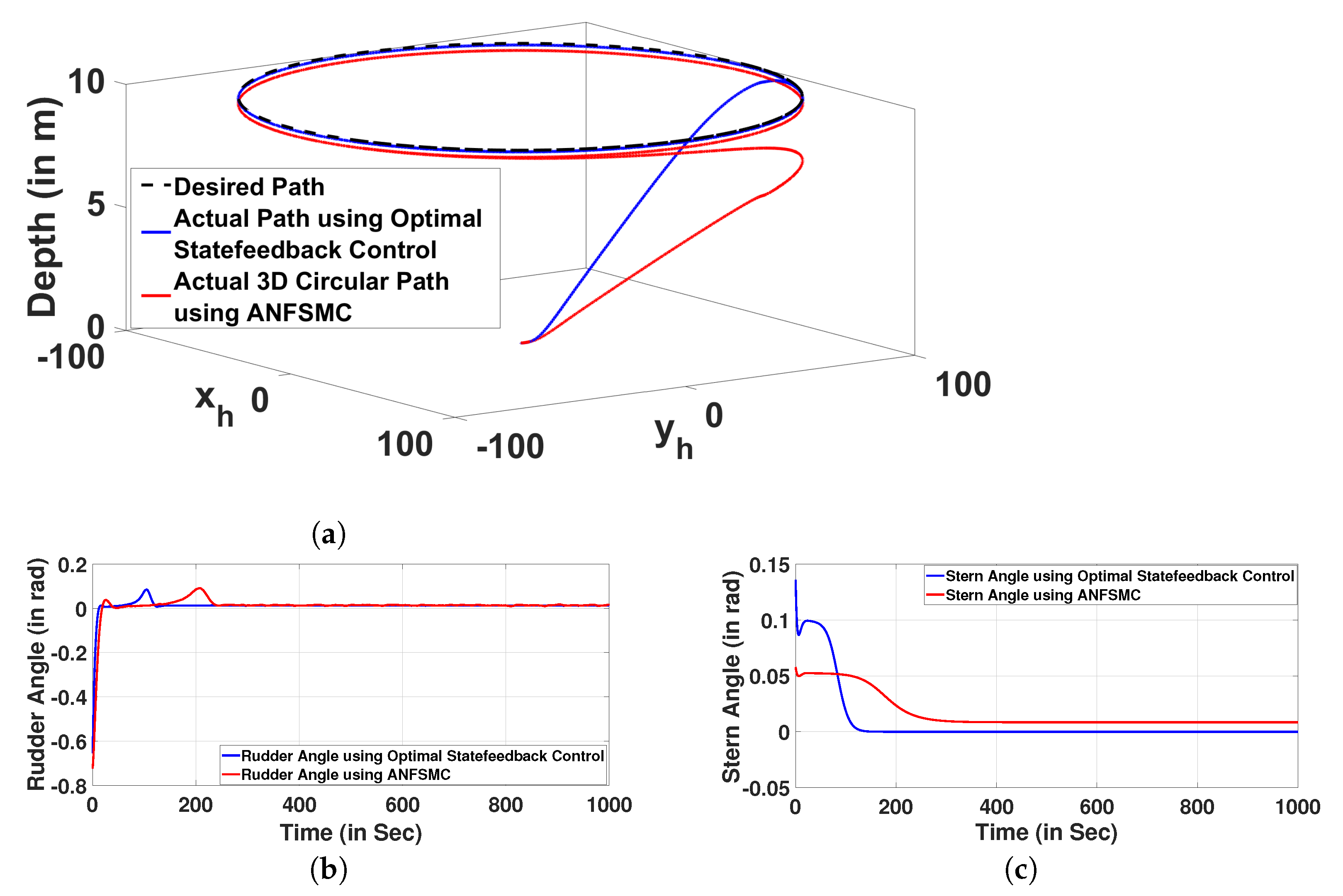
5.2. 3D Path Following

This section shows the tracking of a desired circular path which is considered at a constant depth of $z_D=10m$. For the desired path, the path coordinates are considered as $x_D\left(c_a\right)$ and $y_D\left(c_a\right)$. To evaluate the required parameters, the path curvature $c_a$ is involved in designing the yaw orientation as discussed below

$$\begin{array}{c}\hfill \begin{array}{ccc}\hfill {\psi }_t\left(c_a\right)& =\hfill & \hfill arctan\frac{{\left(y_D\right)}^{{}^{\prime }}}{{\left(x_D\right)}^{{}^{\prime }}}\\ \hfill p_e\left(c_a\right)& =\hfill & \hfill \frac{d{\psi }_t\left(c_a\right)}{d{c}_a}\\ \hfill {\dot{\psi }}_t& =\hfill & \hfill p_e\left(c_a\right){\dot{c}}_a\end{array}\end{array}$$

where ${\left(x_D\right)}^{{}^{\prime }}=\frac{d{x}_D}{d{c}_a}$ and ${\left(y_D\right)}^{{}^{\prime }}=\frac{d{y}_D}{d{c}_a}$. The simulation for the path following control is performed by considering $u_h$ = 2 m/s and $\eta$ = 10 which is a positive design parameter and termed as look ahead distance. The desired path coordinates are given by

$$\begin{array}{c}\hfill x_D\left(c_a\right)=100cos\left(0.01c_a\right),y_D\left(c_a\right)=100sin\left(0.01c_a\right)\end{array}$$

The desired coordinates for circular path tracking of AURV in a 3D plane are shown in Figure 9. As indicated in the figure, the initial position of the AURV is considered as [0,0,10]. Referring to Figure 9a, it is observed that the proposed optimal state feedback control tracks the desired circular path by achieving the desired depth. While in the case of ANFSMC control, it is seen that the AURV is taking more time to reach the desired depth in tracking the desired circular path. A deviation in tracking the desired 3D circular path can be observed in the case of ANFSMC control. Figure 9b,c present the rudder and stern movement respectively. In both cases, the proposed control algorithm performs better compared to ANFSMC.

6. Conclusions

A state feedback approach for an AURV system using a polytopic approach is discussed in this paper. The state feedback control law is developed by considering a polytopic uncertain system that is formulated using the selected hydrodynamic parameters of AURV in both horizontal and vertical planes. Besides, separate backstepping control algorithms for the kinematics of AURV are designed in both horizontal and vertical planes. Furthermore, a control structure is developed from the decoupled models of AURV to achieve the 3D path following task. The effectiveness of the developed control algorithm is verified by implementing it for different paths. From the results, it is observed that the control effort generated by the control algorithm is minimal compared to the ANFSMC algorithm. Besides, the error is minimum in the case of the proposed control algorithm as compared to the ANFSMC algorithm. The polytopic model is designed using $\pm 10\%$ uncertainty on selected hydrodynamic parameters in order to ensure the robust behaviour of the closed loop system. The developed control law depicts the tracking of the desired circular path in the presence of uncertain hydrodynamic parameters. The path error coordinates are minimized to achieve the desired tracking of the path. The simulation studies are carried out in MATLAB/Simulink environment using the YALMIP tool.

References

1. Santhakumar, M.; Asokan, T. Investigations on the hybrid tracking control of an underactuated autonomous underwater robot. Adv. Robot. 2010, 24, 1529–1556. [Google Scholar] [CrossRef]
2. Zhang, L.; Jia, H.; Jiang, D. Sliding mode prediction control for 3d path following of an underactuated auv. IFAC Proc. Vol. 2014, 47, 8799–8804. [Google Scholar] [CrossRef] [Green Version]
3. Cui, R.; Zhang, X.; Cui, D. Adaptive sliding-mode attitude control for autonomous underwater vehicles with input nonlinearities. Ocean. Eng. 2016, 123, 45–54. [Google Scholar] [CrossRef]
4. Yang, X.; Zhu, X.; Liu, W.; Ye, H.; Xue, W.; Yan, C.; Xu, W. A Hybrid Autonomous Recovery Scheme for AUV Based Dubins Path and Non-Singular Terminal Sliding Mode Control Method. IEEE Access 2022, 10, 61265–61276. [Google Scholar] [CrossRef]
5. Lakhekar, G.; Waghmare, L. Robust self-organising fuzzy sliding mode-based path-following control for autonomous underwater vehicles. J. Mar. Eng. Technol. 2022, 1–22. [Google Scholar] [CrossRef]
6. You, S.; Lim, T.; Jeong, S. General path-following manoeuvres for an underwater vehicle using robust control synthesis. Proc. Inst. Mech. Eng. Part I J. Syst. Control. Eng. 2010, 224, 960–969. [Google Scholar] [CrossRef]
7. Mahapatra, S.; Subudhi, B. Design of a steering control law for an autonomous underwater vehicle using nonlinear H state feedback technique. Nonlinear Dyn. 2017, 90, 837–854. [Google Scholar] [CrossRef]
8. Mahapatra, S.; Subudhi, B. Design and experimental realization of a backstepping nonlinear H control for an autonomous underwater vehicle using a nonlinear matrix inequality approach. Trans. Inst. Meas. Control 2018, 40, 3390–3403. [Google Scholar] [CrossRef]
9. Mahapatra, S.; Subudhi, B.; Rout, R. Diving control of an Autonomous Underwater Vehicle using nonlinear H measurement feedback technique. In Proceedings of the OCEANS 2016, Shanghai, China, 10–13 April 2016; pp. 1–5. [Google Scholar]
10. Mahapatra, S.; Subudhi, B. Nonlinear matrix inequality approach based heading control for an autonomous underwater vehicle with experimental realization. IFAC J. Syst. Control 2021, 16, 100138. [Google Scholar] [CrossRef]
11. Mahapatra, S.; Subudhi, B.; Rout, R.; Kumar, B. Nonlinear H control for an autonomous underwater vehicle in the vertical plane. IFAC-PapersOnLine 2016, 49, 391–395. [Google Scholar] [CrossRef]
12. Mahapatra, S.; Subudhi, B. Nonlinear H state and output feedback control schemes for an autonomous underwater vehicle in the dive plane. Trans. Inst. Meas. Control 2018, 40, 2024–2038. [Google Scholar] [CrossRef]
13. Cao, X.; Zhu, D.; Yang, S. Multi-AUV target search based on bioinspired neurodynamics model in 3-D underwater environments. IEEE Trans. Neural Netw. Learn. Syst. 2015, 27, 2364–2374. [Google Scholar] [CrossRef]
14. Sun, Y.; Zhang, C.; Zhang, G.; Xu, H.; Ran, X. Three-dimensional path tracking control of autonomous underwater vehicle based on deep reinforcement learning. J. Mar. Sci. Eng. 2019, 7, 443. [Google Scholar] [CrossRef] [Green Version]
15. Xiong, C.; Chen, D.; Lu, D.; Zeng, Z.; Lian, L. Path planning of multiple autonomous marine vehicles for adaptive sampling using Voronoi-based ant colony optimization. Robot. Auton. Syst. 2019, 115, 90–103. [Google Scholar] [CrossRef]
16. Cao, X.; Xu, X. Hunting algorithm for multi-auv based on dynamic prediction of target trajectory in 3d underwater environment. IEEE Access 2020, 8, 138529–138538. [Google Scholar] [CrossRef]
17. Zhang, W.; Shen, P.; Qi, H.; Zhang, Q.; Ma, T.; Li, Y. AUV Path Planning Algorithm for Terrain Aided Navigation. J. Mar. Sci. Eng. 2022, 10, 1393. [Google Scholar] [CrossRef]
18. Gan, W.; Zhu, D.; Ji, D. QPSO-model predictive control-based approach to dynamic trajectory tracking control for unmanned underwater vehicles. Ocean. Eng. 2018, 158, 208–220. [Google Scholar] [CrossRef]
19. Cho, H.; Kim, B.; Yu, S.-C. AUV-Based Underwater 3-D Point Cloud Generation Using Acoustic Lens-Based Multibeam Sonar. IEEE J. Ocean. Eng. 2018, 43, 856–872. [Google Scholar] [CrossRef]
20. Xu, R.; Tang, G.; Han, L.; Xie, D. Trajectory tracking control for a CMG-based underwater vehicle with input saturation in 3D space. Ocean Eng. 2019, 173, 587–598. [Google Scholar] [CrossRef]
21. Yao, X.; Wang, X. Integral vector field control for three-dimensional path following of autonomous underwater vehicle. J. Mar. Sci. Technol. 2021, 26, 159–173. [Google Scholar] [CrossRef]
22. Xiang, X.; Yu, C.; Zhang, Q. Robust fuzzy 3D path following for autonomous underwater vehicle subject to uncertainties. Comput. Oper. Res. 2017, 84, 165–177. [Google Scholar] [CrossRef]
23. Yu, C.; Xiang, X.; Lapierre, L.; Zhang, Q. Nonlinear guidance and fuzzy control for three-dimensional path following of an underactuated autonomous underwater vehicle. Ocean. Eng. 2017, 146, 457–467. [Google Scholar] [CrossRef] [Green Version]
24. Liang, X.; Qu, X.; Wan, L.; Ma, Q. Three-dimensional path following of an underactuated AUV based on fuzzy backstepping sliding mode control. Int. J. Fuzzy Syst. 2018, 20, 640–649. [Google Scholar] [CrossRef]
25. Zhang, Y.; Wang, X.; Wang, S.; Miao, J. DO-LPV-based robust 3D path following control of underactuated autonomous underwater vehicle with multiple uncertainties. ISA Trans. 2020, 101, 189–203. [Google Scholar] [CrossRef]
26. Lei, M.; Li, Y.; Pang, S. Robust singular perturbation control for 3D path following of underactuated AUVs. Int. J. Nav. Archit. Ocean. Eng. 2021, 13, 758–771. [Google Scholar] [CrossRef]
27. Rezazadegan, F.; Shojaei, K.; Sheikholeslam, F.; Chatraei, A. A novel approach to 6-DOF adaptive trajectory tracking control of an AUV in the presence of parameter uncertainties. Ocean. Eng. 2015, 107, 246–258. [Google Scholar] [CrossRef]
28. Li, Y.; Wei, C.; Wu, Q.; Chen, P.; Jiang, Y.; Li, Y. Study of 3 dimension trajectory tracking of underactuated autonomous underwater vehicle. Ocean. Eng. 2015, 105, 270–274. [Google Scholar] [CrossRef]
29. Liang, X.; Wan, L.; Blake, J.; Shenoi, R.; Townsend, N. Path following of an underactuated AUV based on fuzzy backstepping sliding mode control. Int. J. Adv. Robot. Syst. 2016, 13, 122. [Google Scholar] [CrossRef] [Green Version]
30. Cervantes, J.; Yu, W.; Salazar, S.; Chairez, I.; Lozano, R. Output based backstepping control for trajectory tracking of an autonomous underwater vehicle. In Proceedings of the 2016 American Control Conference (ACC), Boston, MA, USA, 6–8 July 2016; pp. 6423–6428. [Google Scholar]
31. He, Y.; Wu, M.; She, J. Improved bounded-real-lemma representation and H control of systems with polytopic uncertainties. IEEE Trans. Circuits Syst. II Express Briefs 2005, 52, 380–383. [Google Scholar]
32. Karimi, A.; Sadabadi, M. Fixed-order controller design for state space polytopic systems by convex optimization. IFAC Proc. Vol. 2013, 46, 683–688. [Google Scholar] [CrossRef] [Green Version]
33. Helwa, M.; Lin, Z.; Broucke, M. On the necessity of the invariance conditions for reach control on polytopes. Syst. Control Lett. 2016, 90, 16–19. [Google Scholar] [CrossRef]
34. Vesely, V.; Ilka, A. Generalized robust gain-scheduled PID controller design for affine LPV systems with polytopic uncertainty. Syst. Control Lett. 2017, 105, 6–13. [Google Scholar] [CrossRef] [Green Version]
35. Hosoe, Y.; Hagiwara, T.; Peaucelle, D. Robust stability analysis and state feedback synthesis for discrete- time systems characterized by random polytopes. IEEE Trans. Autom. Control 2017, 63, 556–562. [Google Scholar] [CrossRef]
36. Tognetti, E.; Calliero, T.; Jungers, M. Output feedback control for bilinear systems: A polytopic approach. IFAC-PapersOnLine 2019, 52, 58–63. [Google Scholar] [CrossRef]
37. Jirasek, R.; Schauer, T.; Bleicher, A. Active Vibration Control of a Convertible Structure based on a Polytopic LPV Model Representation. IFAC-PapersOnLine 2020, 53, 8389–8394. [Google Scholar] [CrossRef]
38. Goyal, J.; Aggarwal, S.; Ghosh, S.; Kamal, S.; Dworak, P. L2-based static output feedback controller design for a class of polytopic systems with actuator saturation. Int. J. Control 2021, 95, 2151–2163. [Google Scholar] [CrossRef]
39. Yamashita, Y.; Matsukizono, R.; Kobayashi, K. Asymptotic stabilization of nonlinear systems with convex-polytope input constraints by continuous input. Automatica 2022, 138, 110032. [Google Scholar] [CrossRef]
40. Lakhekar, G.; Waghmare, L.; Jadhav, P.; Roy, R. Robust diving motion control of an autonomous underwater vehicle using adaptive neuro-fuzzy sliding mode technique. IEEE Access 2020, 8, 109891–109904. [Google Scholar] [CrossRef]
41. Zhang, J.; Swain, A.K.; Nguang, S.K. Robust Observer-Based Fault Diagnosis for Nonlinear Systems Using MATLAB®; Springer: Berlin, Germany, 2016. [Google Scholar]
42. Silvestre, C.; Pascoal, A. Control of the INFANTE AUV using gain scheduled static output feedback. Control Eng. Pract. 2004, 12, 1501–1509. [Google Scholar] [CrossRef]
43. Fossen, T. Guidance and Control of Ocean Vehicles. Ph.D. Thesis, University of Trondheim, Trondheim, Norway; Printed By John Wiley & Sons: Chichester, UK, 1999; ISBN 0 471 94113 1. [Google Scholar]
Figure 1. Structure of AURV based on Reference Frames.
Jmse 11 00277 g001
Figure 2. Different planes of AURV.
Jmse 11 00277 g002
Figure 3. Controller Configuration in 3D Plane.
Jmse 11 00277 g003
Figure 4. Description of S-F Frame in steering plane.
Jmse 11 00277 g004
Figure 5. Control of depth for ± 10 % uncertainty. (a) Tracking of Desired Depth, (b) Control Input, (c) Pitch Rate, (d) Error Signal.
Jmse 11 00277 g005
Figure 6. Path Following in Vertical Plane for ± 10 % Uncertainty. (a) Tracking of Desired Sine Wave, (b) Control Input for a Sine wave, (c) Pitch Rate for a Sine Wave, (d) Error Signal for a Sine wave.
Jmse 11 00277 g006
Figure 7. Control of yaw for ± 10 % uncertainty. (a) Tracking of Desired Yaw, (b) Control Input, (c) Yaw Rate, (d) Error Signal.
Jmse 11 00277 g007
Figure 8. Path Following in Horizontal Plane for ± 10 % Uncertainty. (a) Tracking of Desired Spline Path, (b) Control Input for a Spline Path, (c) x-axis path error for spline path, (d) y-axis path error for spline path.
Jmse 11 00277 g008
Figure 9. 3D Path Following for Circular Path for ± 10 % Uncertainty. (a) 3D Plane Path Following, (b) Rudder Angle, (c) Stern Angle.
Jmse 11 00277 g009