Research on Carbon Intensity Prediction Method for Ships Based on Sensors and Meteorological Data

Abstract

The Carbon Intensity Index (CII) exerts a substantial impact on the operations and valuation of international shipping vessels. Accurately predicting the CII of ships could help ship operators dynamically evaluate the possible CII grate of a ship at the end of the year and choose appropriate methods to improve its CII grade to meet the IMO requirement with minimum cost. This study developed and compared five CII predicting models with multiple data sources. It integrates diverse data sources, including Automatic Identification System (AIS) data, sensor data, meteorological data, and sea state data from 2022, and extracts 21 relevant features for the vessel CII prediction. Five machine learning methods, including Artificial Neural Network (ANN), Support Vector Regression (SVR), Least Absolute Shrinkage and Selection Operator (LASSO), Extreme Gradient Boosting (XGBoost), and Random Forest (RF), are employed to construct the CII prediction model, which is then applied to a 2400 TEU container ship. Features such as the mean period of total swell, mean period of wind waves, and seawater temperature were considered for inclusion as inputs in the model. The results reveal significant correlations between cumulative carbon emissions intensity and features like cumulative distance, seawater temperature, wave period, and swell period. Among these, the strongest correlations are observed with cumulative distance and seawater temperature, having correlation coefficients of 0.45 and 0.34, respectively. Notably, the ANN model demonstrates the highest accuracy in CII prediction, with an average absolute error of 0.0336, whereas the LASSO model exhibits the highest error of 0.2817. Similarly, the ANN model provides more accurate annual CII ratings for the vessel. Consequently, the ANN model proves to be the most suitable choice for cumulative CII prediction.

1. Introduction

The IMO Marine Environment Protection Committee (MEPC 76), which took place in June 2021, introduced the Carbon Intensity Indicator (CII). This indicator is defined as the total amount of CO₂ emissions divided by the deadweight and the distance traveled per year. According to the requirements of the International Maritime Organization (IMO), starting from 1 January 2023, ships of 5000 GT or above on international voyages will be required to determine their operational carbon intensity indicator (CII) rating, and the CII rating requirement will be increased by 2% per year until 2026. After that time, the CII rating requirement is likely to be further increased to meet the requirements of the IMO 2023 international shipping greenhouse gas emission reduction strategy [1]. The CII ratings of ships are categorized into five classes from high to low: A, B, C, D, and E. Ships need to have a CII rating of at least C. If a ship is rated E, or if a ship has been rated D for three consecutive years, a corrective action plan needs to be developed as part of the ship’s energy efficiency management plan [2].

In addition, as CII rating starts affecting the price and contract of ship chartering, a number of CII-related clauses have been added to the charter party. For example, the burden of CII is solely with the charterer [3]. If a chartered vessel does not have a CII rating of C, it may result in a breach of contract, leading to financial loss for the charterer. Increased waiting time in port, vessel idling, and charter suspension may have a negative impact on a ship’s carbon intensity [4]. It is important for shipowner or operators to dynamically monitor and manage ship CII rating.

It is prudent for shipowners to monitor and assess the ship’s actual CII in real time in order to determine how close it is to the required CII and to take appropriate measures and actions to avoid getting into a situation that would result in a lower CII rating [4]. Accurate prediction of the carbon intensity of a ship is an important basis for the future control of the CII rating of a ship. Previous studies are mainly focused on calculating and predicting ship fuel consumption, and very few studies investigate the prediction of ship CII prediction and upgrading.

Accurate prediction of the CII of a ship enables the assessment of the year-to-year change in CII grade of the ship. This foresight allows proactive measures to be taken, ensuring compliance with the annual carbon intensity qualification. Such proactive management not only aids in reducing carbon emissions and energy consumption but is also crucial in chartering contracts. Precise CII prediction prevents shipowners from incurring liquidated damage costs by ensuring the ship’s carbon intensity level is maintained within the contractual requirements.

The main purpose of this work is to investigate the performance of five machine learning models for carbon intensity prediction using multiple data sources, including AIS data, fuel flow sensor data, meteorological data and sea state data, to identify the most suitable models for carbon intensity prediction. The best model will be utilized to further predict the CII rating at the end of the year. One container ship is taken as an example to illustrate the development process. This work first analyzes the change in carbon intensity of ships over a one-year period by using a carbon intensity assessment methodology. Second, the carbon intensity obtained from this assessment method is used as a prediction target to compare different machine learning models for carbon intensity prediction. This paper also analyzes the correlation between factors affecting fuel consumption and carbon intensity. The ultimate goal of this paper is to assess the accuracy of the carbon intensity classes obtained from the prediction using machine learning models.

This paper focuses on the urgent need for an annual rating of CII of ship operation. Taking a container ship with a capacity of about 2400 TEU as an example, this study uses the ship’s AIS data, real-time fuel consumption data, sensor data, and meteorological data from 2022 to compare and analyze the accuracy of the different machine learning methods for predicting the CII of the ship to provide support for the prediction of CII for the ship and the ship’s annual rating.

The remainder of this paper is organized as follows. Section 2 reviews related works on the prediction of fuel consumption and carbon intensity, while Section 3 introduces the main datasets used in our study and describes the processes and methods used to predict CII. Section 4 presents and discusses the results of the study. Finally, conclusions, limitations, and future work are presented in Section 5.

2. Related Work

Currently, related research in the same field consists of studies on the prediction of fuel consumption of ships, the prediction of resistance, and how to improve the carbon intensity level. However, there are fewer studies on the prediction of carbon intensity of ships, while most scholars have conducted studies on the prediction of fuel consumption and resistance of ships, and machine learning models have been frequently used for the prediction.

Wang carried out feature compression of the ship energy consumption data by means of the LASSO regression algorithm, and the results showed that the prediction effect of LASSO is better than neural network, support vector regression, and other models [5]. Jeon proposed a regression model based on an artificial neural network that adjusted the hyperparameters of the neural network, such as hidden layer, neuron, activation function and other hyperparameters. And the results showed that ANN has a higher prediction accuracy than the polynomial regression and support vector machine in fuel consumption prediction [6]. Ren compared the prediction results under different data sources using a ridge regression model based on AIS data, MRV data, and MRV-normalized data, respectively, and found that the model based on MRV report achieved the best results [7]. Li investigated the results of various prediction models with different combinations of data sources based on a variety of data sources, such as logbooks, meteorological data, and AIS data [8,9,10]. Uyanık proposed the methods of kernel ridge regression, Bayesian ridge regression, and Adaboost, and found that the ridge regression model had a higher accuracy [11]. In summary, different models are used to study the prediction of ship fuel consumption. The research methods are mainly based on neural networks, support vector machines, LASSO regression, and integrated learning models [12,13]. Under different scenarios and datasets, the best prediction models are different. In the area of resistance prediction, Yidiz presented a method for predicting the residual drag coefficient of a trimaran using artificial neural networks that had parameters such as lateral and longitudinal positions of the side hulls, longitudinal buoyancy centers, and Froude number [14]. Martić successfully applied artificial neural networks to the assessment of additional resistance on container ships [15].

In terms of carbon intensity, previous studies are mainly focused on how to upgrade ships to make them more efficient and attractive to charterers and to increase their competitiveness in the market [16]. Wang analyzes the effectiveness of four current CII metrics and considers designing an average CII calculation method for shipping companies rather than individual vessels [17]. Gianni considered a 180,000 GRT cruise ship as a case ship and designed seven scenarios to calculate the CII with reference to its power plant, then analyzed the impact of solid oxide fuel cells (SOFC) on the CII [18]. Hoffmann analyzed the connection between biofouling and ship CII and provided insights and strategies for improving hull performance related to the use of antifouling coatings [19]. During the gap period when the industry was waiting for alternative fuel solutions [20], Bayrakta designed seven different scenarios to test the EEXI and CII values of different vessels with different engine configurations and analyzed the impact of the utilization of two alternative fuels, LNG and methanol, on the EEXI and CII by calculating the EEXI and CII values of the vessels for the years 2019 to 2026 [21]. In addition, some studies have developed mathematical models to analyze the factors affecting carbon intensity. Elkafas found that carbon intensity values depend on the number of trips per year, the number of passengers carried, and the amount of fuel consumed, and that proper deceleration reduces the ship’s emission rate [22]. Sun modeled the speed of a time-chartered vessel with CII penalties included and found that the larger the vessel, the more carbon emissions, and that carbon intensity and CII penalties are reduced when the charter speed is reduced for the same amount of time [23].

In general, compared with studies on fuel consumption, research on carbon intensity and CII grating are relatively rare; those that exist are mainly focused on factors that affect CII grading and how to upgrade CII level. Studies on how to predict CII and CII grating are still very limited. Although the fuel consumption of ships is closely related to the carbon intensity of a ship’s operation, it is still rare to find studies that use the carbon intensity of ships as a direct prediction target.

3. Data and Methodology

3.1. Data

3.1.1. Case Ship Data

This study takes a container ship of 2400 TEU as an example. The information related to this container ship is listed in

Table 1. Main information of the analyzed container ship.

Vessel Type	Container
Built	2019
Gross tonnage	26,771
Deadweight	35,337
Length	185
Breadth	32
Number of main engines	1
Main engine power	13,700 kW
Number of auxiliary engines	2
Auxiliary engine power	1370 kW, 1840 kW

. The case ship has one main engine and two auxiliary engines. The main engine provides propulsion power, and the auxiliary engines provide electricity to the ship.

The data sources for this study mainly include AIS data, sensor data, meteorological data, and sea state data.

3.1.2. AIS Data

AIS data provided by shipping companies. The ship’s AIS data include dynamic and static data, and the update frequency differs according to the ship’s speed and position. In addition to vessel identification and specific information (MMSI, Call Sign, Name, Draught, Length, Breadth), AIS data also contains specific navigational data, including Date, Longitude, Latitude, Speed, Course, ROT. AIS data useful for this paper are listed in

Table 2. Main columns and sample data of the AIS data.

Date	Lon	Lat	Course (°)	Speed (kn)	ROT (°/s)	Draught (m)
2022-01-01 00:26:16	123.3059	30.9999	357.0	16.2	348.0	8.7
2022-01-01 00:28:21	123.3048	31.0051	345.0	16.1	340.0	8.7
2022-01-01 00:39:02	123.2830	31.0502	337.0	16.5	335.0	8.7
2022-01-01 00:43:50	123.2739	31.0711	342.0	16.6	339.0	8.7

.

The generation of missing data is necessary due to large amounts of missing information in some areas due to weather and location, which may make it impossible to fully calculate the distance traveled by the case vessel. This paper uses the linear interpolation method to interpolate the information in Table 2 with a time interval of 5 min. According to the change of latitude and longitude of neighboring AIS points, the sailing distance of the ship can be calculated. Data containing sailing distances are listed in

Table 3. AIS data with 5 min sampling and sailing distances.

Date	Lon	Lat	Distance (m)
2022-01-01 00:25:00	123.3054	31.0025	294.5
2022-01-01 00:26:16	123.3059	30.9999	588.9
2022-01-01 00:28:21	123.3048	31.0051	2570.4
2022-01-01 00:30:00	123.2942	31.0263	2858.5

.

Since the frequency of the collected meteorological data and sea state data is hourly, to maintain a uniform time resolution, the ship’s AIS data is aggregated according to the hour in this study [9]. In this paper, the sum of the distances traveled by the case ships and the average of the other data in the AIS data are calculated at intervals of one hour.

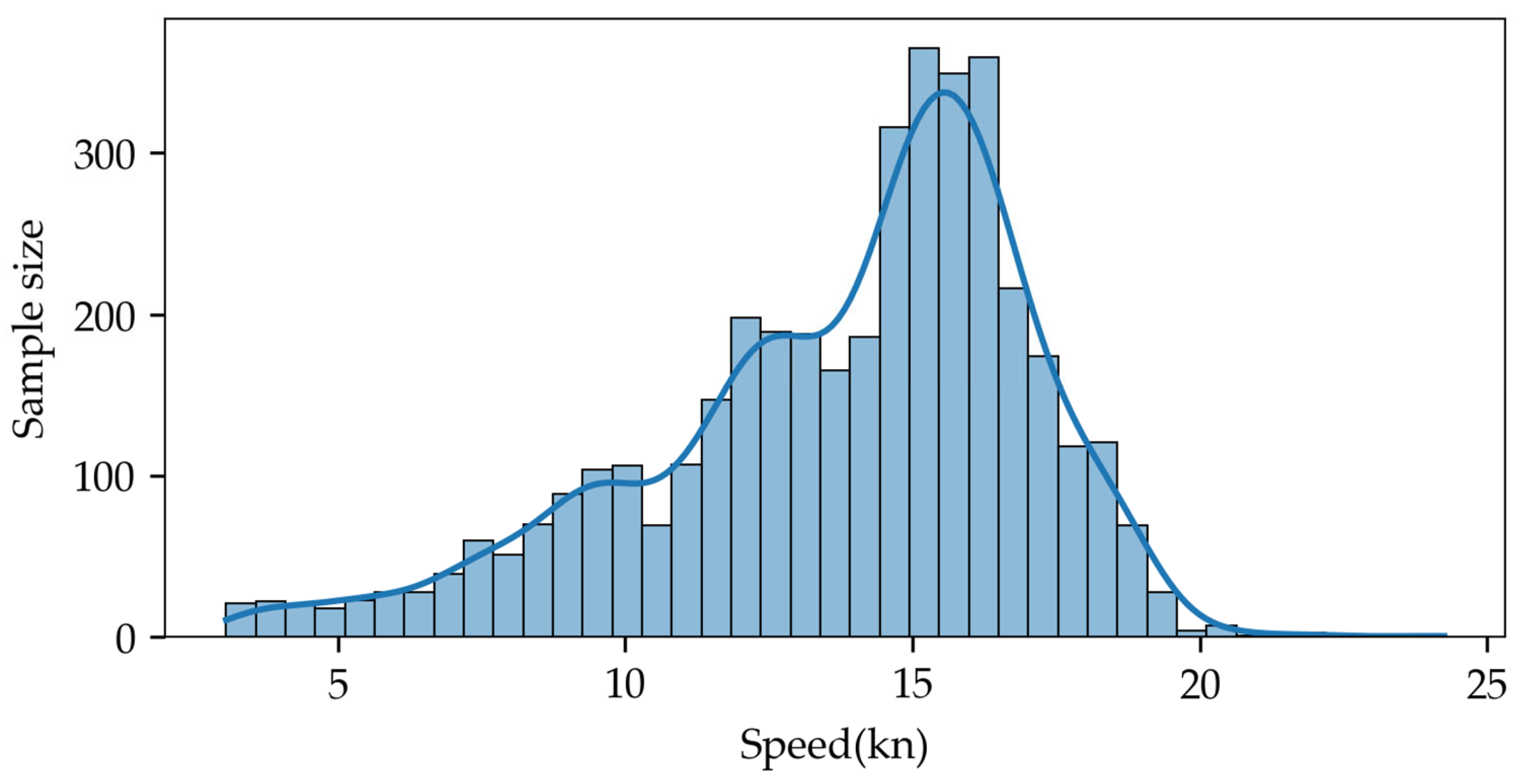
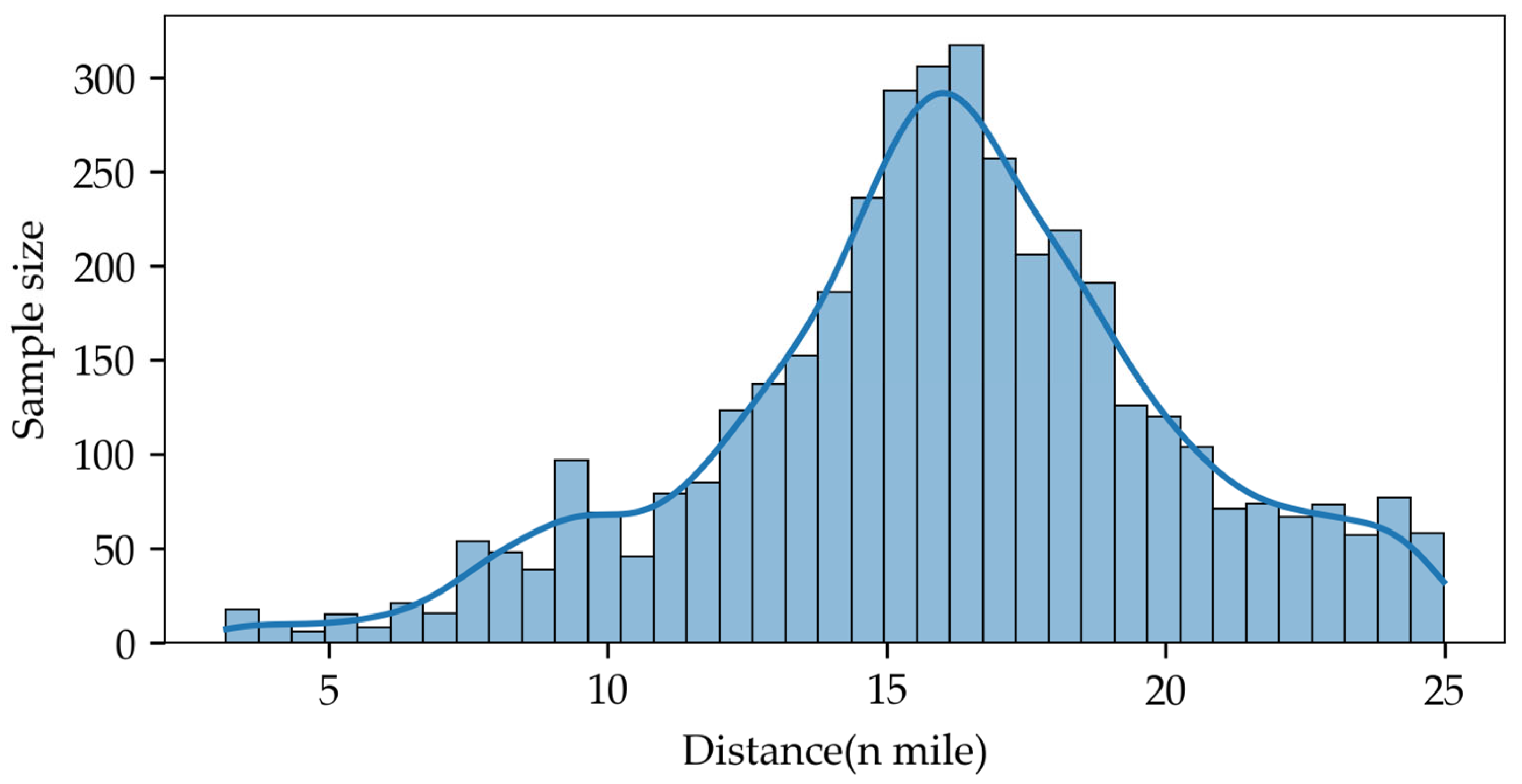
The speed and range data are distributed as shown in Figure 1 and Figure 2 below.

From Figure 1 and Figure 2, it can be found that the data processing ensures the consistency of the distribution of the speed and range data under one hour of data collection frequency. Because of the deviation between the voyage calculated by latitude and longitude in AIS data and the actual voyage, the speed and voyage data in the range of 20~25 do not correspond exactly.

3.1.3. Sensor Data

The case ship is equipped with various sensors to obtain real-time data about the ship. The main engine fuel consumption rate (MEActFOCons), generator fuel consumption rate (DGActFOCons), and boiler fuel consumption rate (BlrActFOCons) are recorded using mass flow meters. The main engine rotational speed (MERpm) and trim of the case ship (Trim) are recorded using the corresponding sensor data. The sensor data used in this paper are listed in

Table 4. Main columns and sample data of sensor data.

PCDate	PCTime	MEActFOCons (kg/h)	DGActFOCons (kg/h)	BlrActFOCons (kg/h)	MERpm (r/min)	Trim (m)
2022-01-01	00:00:03	1256.8874	114.7474	0	81	3.97
2022-01-01	00:00:13	1251.0776	115.6824	0	81	3.06
2022-01-01	00:00:26	1239.1414	116.1036	0	82	3.1
2022-01-01	00:00:36	1238.5380	117.4958	0	82	3.69

.

The original unit of the fuel consumption of the main engine, auxiliary engine, and boiler is kg/h, which needs to be converted into kg according to the time interval of each data point. The converted fuel consumption data are listed in

Table 5. Sensor data with converted fuel consumption data.

PCDate	PCTime	MEActFOCons (kg)	DGActFOCons (kg)	BlrActFOCons (kg)
2022-01-01	00:00:03	1.0474	0.0956	0
2022-01-01	00:00:13	3.4752	0.3213	0
2022-01-01	00:00:26	4.4746	0.4192	0
2022-01-01	00:00:36	3.4403	0.3263	0
2022-01-01	00:00:36	3.4403	0.3263	0

.

To maintain a uniform time resolution for data fusion, the data collected through the sensors also needs to be aggregated on an hourly basis. In this paper, the sum of the fuel consumption and the average of the other data in the sensor data are calculated at intervals of one hour. It was observed that the processed data was found to be less than 8760 (24 × 365) data, so there were also missing values in the sensor data. In this paper, linear interpolation is also taken for the data in the sensor to generate the missing data with a time interval of 1 h. On this basis, the total amount of heavy fuel and light fuel in each hour was calculated, and the total amount of carbon dioxide in each hour was calculated according to the emission factor. Carbon dioxide data are listed in

Table 6. Carbon dioxide emissions at different times.

Date	CO2 (kg)
2022-01-01 00:00:00	4180.33
2022-01-01 01:00:00	4208.82
2022-01-01 02:00:00	4172.76
2022-01-01 03:00:00	4137.75

.

3.1.4. Meteorological and Sea State Data and Processing

In this paper, meteorological and sea state data are obtained from the European Centre for Medium-Range Weather Forecasts (ECMWF) and the Copernicus Marine Service (Copernicus). The data from ECMWF cover a wide range of meteorological data sets from 1979 to present, including wind component at 10 m sea level, temperature, humidity, characteristic wave height, and cycle frequency. The scope of ECMWF data covers several meteorological datasets from 1979 to the present, including the wind component at 10 m above sea level, temperature, humidity, characteristic wave height, and cycle frequency, etc. The scope of Copernicus data covers several sea state datasets for each year, including seawater temperature, the current velocity component at different seawater depths, etc. The meteorological dataset used in this paper was collected at a frequency of 1 h, and the data are downloaded in the form of a grid divided according to latitude and longitude. The collected data information is recorded at each grid point, and there is a wide range of choices for the grid size; the minimum grid density is 0.125° × 0.125°, the maximum grid density is 1° × 1°, and the grid density selected in this paper is 0.25° × 0.25°. The sea state dataset used in this paper was also collected at a frequency of 1 h, and the current velocity component of seawater at a depth of 0.5 m was selected as the basis.

For the processing of meteorological data and sea state data, the latitude and longitude in the AIS data are first utilized to obtain the environmental data corresponding to the ship’s position [8]. Eastward wind speed at 10 m above sea level (u10), northward wind speed at 10 m above sea level (v10), mean direction of total swell (mdts), mean direction of wind waves (mdww), mean period of total swell (mpts), mean period of wind waves (mpww), mean wave direction (mwd), mean wave period (mwp), sea surface temperature (sst), significant_height of combined wind waves and swell (swh), significant height of total swell (shts) and significant height of wind waves (shww) are recorded u ECMWF. Eastward sea water velocity (uo) and northward sea water velocity (vo) are recorded from Copernicus. The environmental data used in this paper are listed in

Table 7. Meteorological data and sea state data from time–space matching acquisition.

Data Name	Sample 1	Sample 2
date	2022-01-01 00:00:00	2022-01-01 01:00:00
u10	−2.4207	−2.6627
v10	0.3611	0.5708
mdts	14.6175	14.2658
mdww	70.0711	91.5424
mpts	6.0399	6.0044
mpww	2.8725	2.1009
mwd	14.6768	14.4249
mwp	6.0288	5.9816
sst	289.3203	288.498
swh	0.9627	0.9532
shts	0.9616	0.9507
shww	0.0295	0.0578
vo	0.1896	0.1587
uo	−0.0190	−0.0428

.

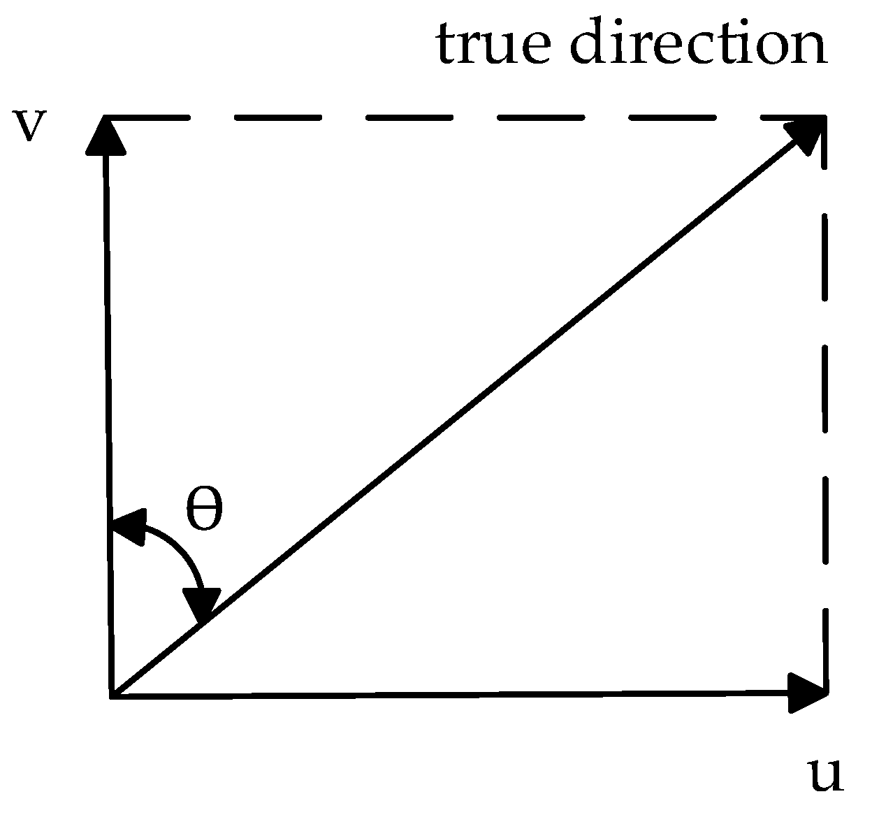
Since the collected wind speed data and flow velocity data are east–west and north–south components, vector synthesis is needed to obtain the actual wind speed, wind direction, current speed, and current direction. The schematic of direction synthesis is shown in Figure 3.

Finally, it is necessary to convert the directions in the meteorological data into the relative directions of the ship in combination with the actual heading of the ship, and further fuse the preprocessed AIS data, sensor data, meteorological data, and sea state data according to the time [9,10].

3.1.5. Calculation of Cumulative Carbon Intensity of Ships

Finally, it is necessary to calculate the cumulative carbon intensity of the ships up to each point of the data, as well as the ratio of the total cumulative CO₂ mass of the ship at each moment in time to the total transport workload it carries out, by using the following formula [16]:

$${\mathrm{CII}}_t=\frac{{\mathrm{M}}_t}{{\mathrm{W}}_t}$$

(1)

where ${\mathrm{M}}_t$ is the total amount of carbon dioxide emission of the ship at the time, in kg and ${\mathrm{W}}_t$ is the total transportation workload accomplished by the ship at the time, in t⋅n mile.

The formula for calculating the total amount of carbon dioxide emission ${\mathrm{M}}_t$ at the time of the ship is as follows:

$${\mathrm{M}}_t={\displaystyle \sum {\mathrm{FC}}_{jt}\times {\mathrm{CF}}_j}$$

(2)

where $j$ is the fuel type; ${\mathrm{FC}}_{jt}$ is the total fuel consumption of the ship at the time, kg; and ${\mathrm{CF}}_j$ is the fuel mass to carbon dioxide mass conversion factor for fuel $j$.

The formula for calculating the total transportation workload of the ship at the time is as follows:

$${\mathrm{W}}_t=\mathrm{C}\times {\mathrm{D}}_t$$

(3)

where $\mathrm{C}$ is the DWT of the ship and ${\mathrm{D}}_t$ is the distance sailed by the ship at the time, n mile.

Equation (1) shows that CII could be calculated from carbon emission, deadweight tons, and sailing distance. Carbon emission could be directly computed by fuel consumption, which is collected through the mass flow meter on the case ship.

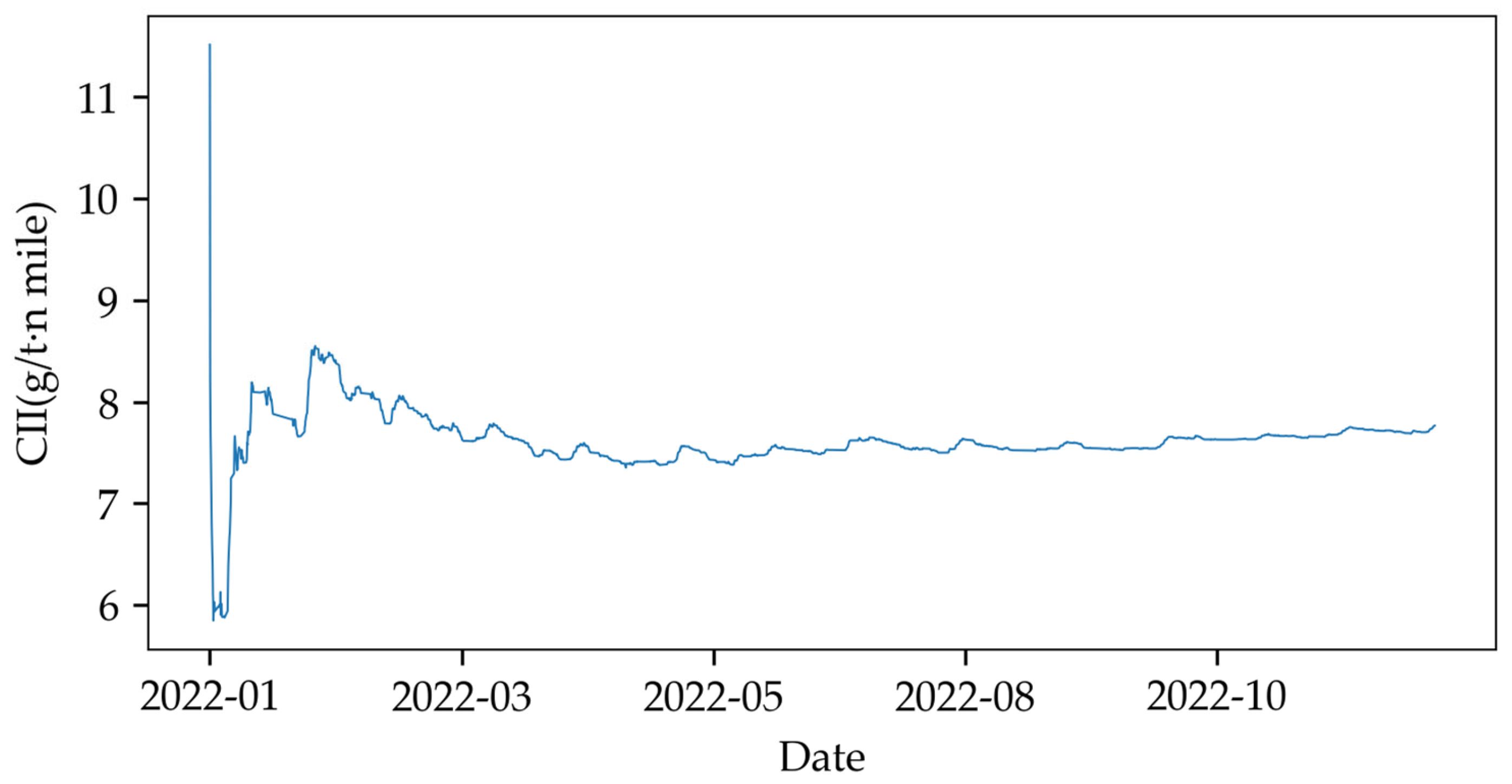
In addition, the variation of CII with time for the ships studied in this paper is shown in Figure 4.

Figure 4 shows that the fluctuations are large in January, but gradually stabilize in the range of 7 to 8 in the time that follows, which occurs because ships start with small voyages and relatively large carbon dioxide emissions, and as the cumulative value of the voyage increases, the calculation of the cumulative CII in conjunction with the deadweight tonnage leads to a certain degree of decrease and stabilization of its future value.

The cumulative CII of the ship mainly focuses on the situation when the ship is in sailing condition. In this paper, it is assumed that a ship is in sailing condition when its speed is more than 3 knots. Therefore, in this study, only data with speed greater than or equal to 3 knots are considered [24]. The total number of processed data is 4061, and some data samples are shown in

Table 8. Sample data of the input for model development.

Data Name	Abbreviation	Data Sources	Unit	Sample 1
speed	speed	AIS	kn	16.4911
rate of turning	rot	AIS	°/s	270.0357
wind speed	wind speed	ECMWF	m/s	2.4476
draught	draught	AIS	m	8.7000
distance	distance	AIS	n mile	10.2731
cumulative value of distance	distance sum	summation	n mile	10.2731
mean period of total swell	mpts	ECMWF	s	6.0399
mean period of wind waves	mpww	ECMWF	s	2.8726
mean period of wave	mwp	ECMWF	s	6.0288
height of combined wind waves and swell	shww	ECMWF	m	0.9628
height of total swell	swh	ECMWF	m	0.9617
height of wind waves	wwh	ECMWF	m	0.0295
current speed	current speed	Copernicus	m/s	0.1906
wind direction	wind direction	vector synthesis	°	4.8576
current direction	current direction	vector synthesis	°	80.6408
swell direction	swell direction	ECMWF	°	100.9890
wind waves direction	dww	ECMWF	°	156.4426
wave direction	wd	ECMWF	°	101.0483
sea surface temperature	sst	ECMWF	℃	16.1703
merpm	merpm	sensors	r/min	81.5403
trim	trim	sensors	m	3.4338
cumulative CII	CII	formula calculation	g/t⋅n mile	11.5154

.

3.2. Methodology

3.2.1. Research Framework

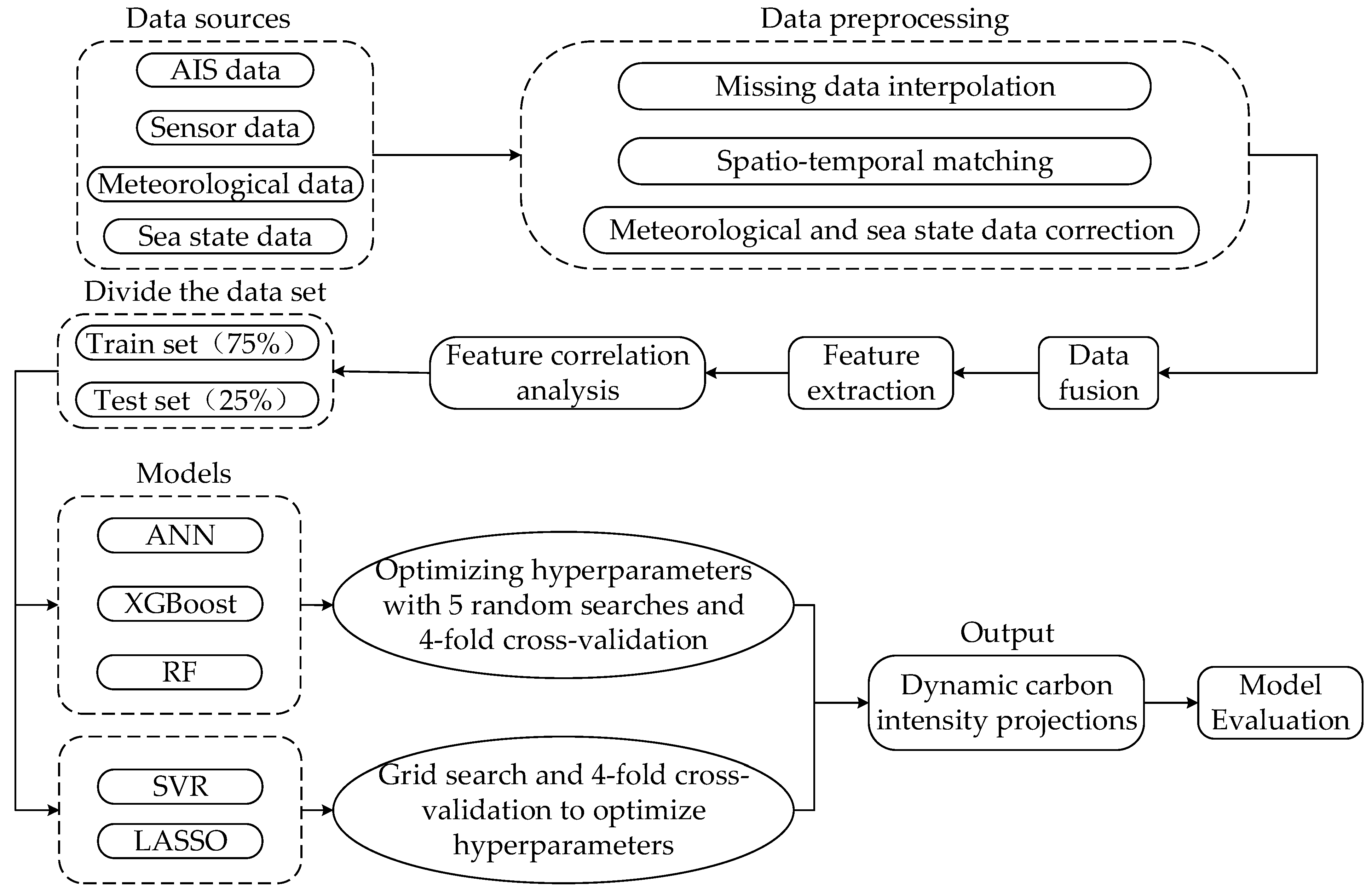
The main research framework could be divided into several steps. First, the ship AIS data, sensor data, and meteorological and sea state data are cleaned and preprocessed, and temporal and spatial fusion are performed. Second, relevant features are extracted, and the correlation between each feature is analyzed. Third, the data are divided into training and testing sets in the ratio of 0.75:0.25 (3046 trainset:1015 test set) according to the time series [25]. Fourth, five machine learning models are used to train and optimize the hyper-parameters of ANN, XGBoost, and RF models by random search and cross-validation, and the parameters of LASSO and SVR are optimized by grid search because of their fewer hyper-parameters. Figure 5 shows the general framework of ship CII prediction.

3.2.2. Model Performance Metrics

In this paper, mean absolute error (MAE), mean square error (MSE), root-mean-square-error (RMSE), and mean absolute percentage error (MAPE) are used to evaluate the performance of the model. The evaluation formulas are calculated as follows:

$$\mathrm{MAE}=\frac{1}{m}\left({\displaystyle \sum _{i=1}^m\left|y_i-{\stackrel{\wedge }{y}}_i\right|}\right)$$

(4)

$$\mathrm{MSE}=\frac{1}{m}{{\displaystyle \sum _{i=1}^m\left(y_i-\stackrel{\wedge }{y_i}\right)}}^2$$

(5)

$$\mathrm{RMSE}=\sqrt{\frac{1}{m}{{\displaystyle \sum _{i=1}^m\left(y_i-\stackrel{\wedge }{y_i}\right)}}^2}$$

(6)

$$\mathrm{MAPE}=\frac{1}{m}{\displaystyle \sum _{i=1}^m\left|\frac{y_i-\stackrel{\wedge }{y_i}}{y_i}\right|}\times 100\%$$

(7)

where $m$ is the number of samples; $y_i$ is the true value; and ${\stackrel{\wedge }{y}}_i$ is the predicted output value of the model.

3.2.3. CII Rating Calculation Model

The carbon intensity rating of a ship must be determined annually using the Carbon Intensity Index (Required CII) of the ship. This is based on the CII reference baseline for a specific ship type for the year 2019, and its rating boundaries are then determined based on the boundary parameters of the ship type. This allows its annual carbon intensity rating to be found. The specific calculation formula is as follows [16]:

$${\mathrm{CII}}_{\mathrm{ref}}=a\cdot {\mathrm{C}}^{-c}$$

(8)

where ${\mathrm{CII}}_{\mathrm{ref}}$ is the reference baseline value of CII in 2019, g/(DWT⋅n mile) or g/(GT⋅n mile); $\mathrm{C}$ is the deadweight tonnage (DWT) of the ship; and $a$ and $c$ are the parameters for the different ship types. Since the research object of this paper is a container ship, $a$ = 1984 and $c$ = 0.489 [18].

The required CII is calculated as follows [26]:

$${\mathrm{CII}}_{\mathrm{Re}\mathrm{q}}=\left(1-\frac{Z}{100}\right)\times {\mathrm{CII}}_{\mathrm{ref}}$$

(9)

where $Z$ is the discount factor of CII for different years; the year of study for this paper is 2022, which has the value of 3 [26]. For the convenience of rating, the rating mechanism is used to define four boundaries per year, which facilitates the division into five grades. Accordingly, the rating can be determined by comparing the annual CII of the ship with the boundary value, and the formula for calculating the boundary value ${\mathrm{B}}_i$ is as follows [27]:

$${\mathrm{B}}_i=\exp \left({\mathrm{d}}_i\right)\cdot {\mathrm{CII}}_{\mathrm{Re}\mathrm{q}}$$

(10)

where $i$ = 1, 2, 3, 4, and $\exp \left({\mathrm{d}}_i\right)$ is the boundary parameter of the container ship. As shown in

Table 9. Carbon intensity rating boundary parameters for container ships.

Ship Type	Capacity	exp(d1)	exp(d2)	exp(d3)	exp(d4)
container ship	DWT	0.83	0.94	1.07	1.19

[27].

4. Results and Discussion

4.1. Feature Correlation Analysis

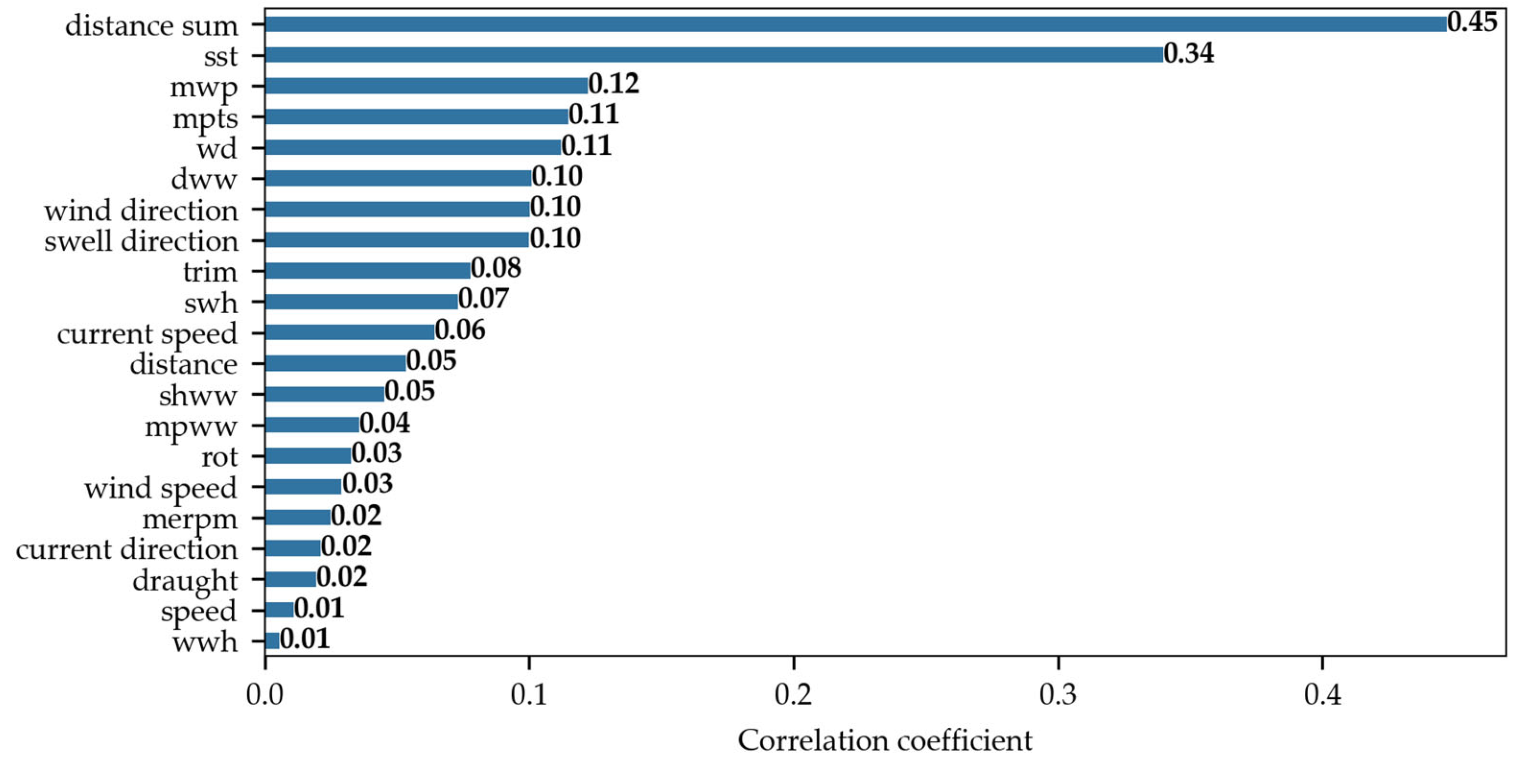
Since the carbon intensity of a ship is calculated based on the ship’s fuel consumption, carbon emission factor, deadweight tonnage, and voyage, this paper extracts 21 relevant features that affect the fuel consumption as inputs to the cumulative carbon intensity prediction model based on the past research [8,9,10,25]. After normalizing all data, the correlation analysis is carried out, as shown in Figure 6. It was found that the correlation between the features, such as seawater temperature, wave period, and swell period, and the cumulative CII of the ship is high, which is different from the results of previous studies. In previous studies [12,28], it was found that the meteorological data, such as navigation speed, main engine speed, and wave height, have significant influence on the fuel consumption of the ship, and the CII of the ship needs to be further calculated according to the fuel consumption data to be obtained. However, Figure 6 shows that characteristics such as speed and engine speed do not show strong correlation with the cumulative CII of the ship. This probably occurs because this paper focuses on the prediction of the cumulative CII, which is calculated by the cumulative carbon emission and cumulative voyage, making it impossible to accurately understand the relationship between the cumulative carbon intensity and characteristics such as speed and engine speed.

4.2. Analysis of Carbon Intensity Prediction Models

In this paper, Windows 11, 12th Gen Intel(R) Core(TM) i7-12700H processor, 16 G RAM, and python version 3.9 were used as the experimental environment. The study takes the cumulative carbon intensity value of the ship as the prediction target and conduct experiments using five machine learning models in both the parameterized and unparameterized cases. In the case of tuning, this paper uses random search and grid search combined with 4-fold cross-validation to optimize the hyper-parameters of ANN, XGBoost, RF and LASSO, SVR models, respectively, in which the search range of the optimizer in the ANN model is (SGD, RMSprop, Adagrad, Adadelta, Adam, Adamax, Nadam), denoted by the abbreviation (S,N), and the search ranges of the remaining hyperparameters, the default values in the case of no parameter tuning, and the search results are shown in

Table 10. Comparison of hyperparameter optimization results of different models.

Models	Hyperparameter Names	Default Values	Search Ranges	1	2	3	4	5
ANN	optimizer	Adam	(S,N)	RMSprop	Adamax	Adamax	RMSprop	Adamax
	neurons	100	(10,100)	40	80	30	100	80
	epochs	100	(10,200)	50	10	100	200	50
	batch_size	32	(10,100)	90	10	40	20	70
SVR	C	1	(0.01,10)	0.1
	gamma	scale	(0.0001,10)	1
LASSO	alpha	1	(0.00001,10)	10
	max_iter	1000	(0,1000)	100
XGBoost	subsample	None	(0.5,1)	0.7	0.6	0.9	0.7	0.8
	n_estimators	100	(0,300)	300	240	233	260	240
	min_child_weight	None	(0,10)	4	7	6	6	7
	max_depth	None	(2,10)	5	4	3	4	3
	learning_rate	None	(0.01,0.3)	0.21	0.3	0.21	0.1	0.21
	gamma	None	(0,10)	0	2	7	6	6
	colsample_bytree	None	(0.5,1)	0.9	0.8	0.9	0.6	0.6
RF	n_estimators	100	(0,300)	233	68	68	266	200
	min_samples_split	2	(1,20)	10	16	17	6	18
	max_depth	None	(2,10)	4	8	4	4	4

.

The evaluation indexes corresponding to the combination of hyperparameters for each optimization of each model were calculated by (4)–(7), as shown in

Table 11. Comparison of predictive performance of models.

Models	Number of Optimizations	MAE	MSE	RMSE	MAPE
ANN	1	0.1179	0.0154	0.1243	1.5333
	2	0.0568	0.0045	0.0673	0.7432
	3 *	0.0476	0.0034	0.0591	0.6186
	4	0.1375	0.0204	0.1431	1.7895
	5	0.0524	0.0040	0.0634	0.6808
	None	0.2181	0.5513	0.7424	2.8392
SVR	1	0.1037	0.0123	0.1109	1.3489
	None	0.4203	0.1946	0.4412	5.4675
LASSO	1	0.2817	0.0864	0.2940	3.6654
	None	0.3687	0.1765	0.4201	3.9968
XGBoost	1	0.1050	0.0127	0.1131	1.3667
	2	0.1083	0.0144	0.1201	1.4091
	3	0.1384	0.0207	0.1439	1.8009
	4	0.0981	0.0112	0.1060	1.2770
	5 *	0.0968	0.0111	0.1055	1.2599
	None	0.1203	0.0161	0.1272	1.5658
RF	1	0.1262	0.0173	0.1317	1.6426
	2 *	0.1213	0.0162	0.1275	1.5777
	3	0.1266	0.0174	0.1322	1.6471
	4	0.1253	0.0171	0.1309	1.6304
	5	0.1262	0.0173	0.1317	1.6422
	None	0.1267	0.0177	0.1331	1.6487

* Indicates the parameter combination with the best performance of the results in the five replicated experiments.

.

The results show that, by repeating the experiments with random search, the ANN, XGBoost and RF models reach the optimum in the third, fifth, and second optimization, respectively, and for any kind of evaluation indexes, the error indexes obtained from the third optimization result of the ANN model are the smallest, and its prediction effect is better than that of the other models, while the performance of the LASSO is the poorest.

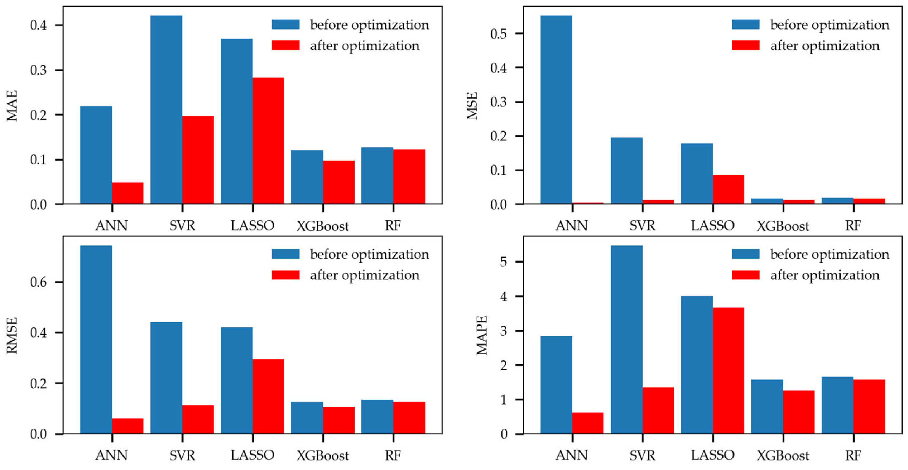
The experiments are carried out without setting the hyperparameters of the model, and the results are visualized and compared with the tuned models; the specific results are shown in Figure 7.

Figure 7 shows that the error metrics of each model decreased after hyperparameter tuning compared to the model with default hyperparameters. Moreover, the tuning has the least enhancement for the XGboost and RF models.

In addition, in order to verify the influence of data dimensions on modeling [8,9,10,29,30] with dataset Set 1 (AIS, sensor, meteorological and sea state data), the above models are used to repeat the experiments five times in the datasets Set 2 (AIS and sensor data), Set 3 (AIS, sensor, meteorological data), and Set 4 (AIS, sensor and sea state data); the optimal parameter combination results are shown in

Table 12. Comparison of model hyperparameter optimization results on different datasets.

Models	Hyperparameter Names	Set 1	Set 2	Set 3	Set 4
ANN	Optimizer	Adamax	Adamax	RMSprop	Nadam
	Neurons	30	40	80	10
	Epochs	100	200	150	200
	batch_size	40	40	90	40
SVR	C	0.1	10	0.1	0.1
	gamma	1	0.0001	1	1
LASSO	Alpha	10	0.0093	6.5793	0.0107
	max_iter	100	1000	100	300
XGBoost	subsample	0.8	0.7	0.9	0.8
	n_estimators	240	200	100	133
	min_child_weight	7	0	5	8
	max_depth	3	5	7	2
	learning_rate	0.21	0.11	0.11	0.21
	Gamma	6	7	1	1
	colsample_bytree	0.6	0.9	0.8	0.5
RF	n_estimators	68	266	233	266
	min_samples_split	16	3	13	13
	max_depth	8	6	6	5

. The comparison results of the optimal prediction performance of different models corresponding to each dataset are shown in

Table 13. Comparison of best prediction performance of model on different datasets.

Models	Data Set	MAE	MSE	RMSE	MAPE
ANN	Set 1	0.0476	0.0034	0.0591	0.6186
	Set 2	0.0336	0.0015	0.0394	0.4377
	Set 3	0.0352	0.0016	0.0410	0.4601
	Set 4	0.0338	0.0017	0.0424	0.4402
SVR	Set 1	0.1037	0.0123	0.1109	1.3489
	Set 2	0.1694	0.0302	0.1739	2.2042
	Set 3	0.1037	0.0123	0.1109	1.3489
	Set 4	0.1037	0.0123	0.1109	1.3489
LASSO	Set 1	0.2817	0.0864	0.2940	3.6654
	Set 2	0.2655	0.0750	0.2738	3.4552
	Set 3	0.2677	0.0761	0.2759	3.4828
	Set 4	0.2652	0.0748	0.2735	3.4509
XGBoost	Set 1	0.0968	0.0111	0.1055	1.2599
	Set 2	0.1293	0.0183	0.1353	1.6828
	Set 3	0.0943	0.0104	0.1024	1.2273
	Set 4	0.1175	0.0155	0.1245	1.5286
RF	Set 1	0.1213	0.0162	0.1275	1.5777
	Set 2	0.1188	0.0157	0.1253	1.5452
	Set 3	0.1169	0.0152	0.1234	1.5207
	Set 4	0.1218	0.0163	0.1280	1.5844

.

Table 13 shows that, by validating different datasets, SVR is less affected by the datasets and has the same performance on Set 1, Set 3, and Set 4 datasets. The rest of the models perform better on the Set 3 dataset after dimensionality reduction, which occur because dimensionality reduction helps the model remove the redundant information, reduces the learning interference of the model, and improves the generalization ability of the model. In addition, compared with other models, the ANN model performs optimally in various situations.

According to the optimal hyper-parameter combinations obtained from each model experiment and input into the model again, the carbon intensity error curves of the ship under the five prediction models are depicted, as shown in Figure 8.

It can be found through Figure 8 that, with each model performing as well as possible, the ANN model predicts the carbon intensity obtained with an error closest to 0, which is the smallest error among the five models.

4.3. Analysis of Carbon Intensity Rating Results

The carbon intensity level boundaries for the case ship can be calculated according to Equation (10), and the results are presented in

Table 14. Carbon intensity rating boundary of container ships.

Boundary	Level
<9.5347	A
9.5347~10.7983	B
10.7983~12.2917	C
12.2917~13.6702	D
>13.6702	E

.

Since this paper divides the training set and test set according to the time series, the last value in the prediction result of each model is selected as the carbon intensity prediction result of the year and compared with the boundary parameters to determine the carbon intensity level achieved in the year, as shown in

Table 15. Comparison of annual carbon intensity errors and ratings across models.

Models	Annual Carbon Intensity	Errors	Level
ANN	7.6330	0.1334	A
SVR	7.5734	0.1930	A
LASSO	7.3699	0.3965	A
XGBoost	7.5383	0.2281	A
RF	7.5431	0.2233	A
Real	7.7664	0	A

.

Table 14 show that the carbon intensity value of the container ship itself for the year 2022 is within the range of 9.5347, and the prediction error value of the model will not be too large; the result is that the predicted carbon intensity value of each model is within the range of 9.5347, and therefore, the rating results of each model are in line with the actual results. In addition, the annual carbon intensity value predicted by the ANN model has the smallest error with the actual value, so the ANN model is more suitable for predicting the carbon intensity of ships.

According to the results of the study, all models predicted carbon intensity within acceptable limits. In addition, since past studies did not analyze the factors affecting the carbon intensity of ships in depth, and the carbon intensity was calculated from fuel consumption, this study considers the relevant factors affecting the fuel consumption as the input features of the models in this paper. Since this paper considers cumulative carbon intensity as a prediction target, it is difficult to construct a strong correlation between fuel consumption characteristics and cumulative carbon intensity in terms of feature correlation.

In terms of carbon intensity prediction, five machine learning models commonly used in the past are selected for prediction in this paper. Since it is unknown under which combination of data the model achieves the highest accuracy, this paper divides the preprocessed data into four categories (Set 1: AIS, sensor, meteorological, and sea state data, Set 2: AIS and sensor data, Set 3: AIS, sensor, and meteorological data, and Set 4: AIS, sensor, and sea state data) and analyzes how the weather and sea state data affect the carbon intensity prediction model. In addition, this paper also gives specific instructions for setting and adjusting the hyperparameters of the model, and the hyperparameter tuning also proves to be effective for the carbon intensity prediction model.

This paper diverges from prior studies in several key aspects. First, it focuses on carbon intensity as the prediction target, in contrast to past studies that predominantly addressed fuel consumption. Second, in terms of feature selection, this paper incorporates factors such as the mean period of total swell, mean period of wind waves, mean period of waves, and seawater temperature; these features were not extensively explored in previous research. Third, in model comparison, the study evaluates the impact of different data combination scenarios on model performance, a consideration often overlooked in prior studies. Unlike previous research on carbon intensity, this paper introduces a cumulative carbon intensity assessment methodology. This methodology analyzes the change in carbon intensity for the selected vessels over a one-year period. Furthermore, the paper successfully applies a machine learning model to predict a ship’s annual carbon intensity, providing insight into the carbon intensity level projected by the model.

This study could be beneficial to the shipping industry in several aspects. First, the proposed predicting method could be used by ship operators to dynamically calculate and monitor the carbon intensity of their ships. Second, carbon intensity prediction could further combine with history operation data to dynamically predict the CII grade of each ship at the end of each year. Third, providing reliable data support allows the ship company to adjust operation strategy or select decarbonization technologies that can upgrade the CII level to meet IMO requirements with minimum costs.

5. Conclusions

The CII grades of ships are crucial to international shipping companies. Failing to meet the CII requirements of IMO or charter contacts will cause dramatical market share and economic losses. This study investigates the performance of five different machine learning methods in predicting ship carbon intensity, including SVR, LASSO regression, XGBoost, and RF models, as well as the ANN model. Multiple data sources, such as AIS data, fuel flow sensor data, and meteorological and sea state data are considered to develop these models.

The results show that, compared with SVR, LASSO regression, XGBoost, and RF models, the ANN model performs the best, and the errors of all four evaluation indexes are minimized. Through several stochastic search optimization experiments, a better combination of hyperparameters can be found, which effectively improves the performance of the ship carbon intensity prediction model. By verifying the performance of the model on different datasets, appropriate dimensionality reduction can improve the accuracy of the ship carbon intensity prediction model. In the annual carbon intensity rating, the annual carbon intensity value predicted by the ANN model is the closest to the real value, while the error of the LASSO model is the largest, and the rating results are consistent with the actual results. The findings of this paper can help enterprises analyze the change of carbon intensity of a ship within a year and determine whether the annual carbon intensity value of a ship is within the qualified range or not. If the predicted carbon intensity grade of a ship is lower than C grade, the shipping company may have to take measures in advance to reduce the carbon intensity.

This is one of the first studies focus on predicting ship CII with multiple machine learning methods and high temporal and spatial data sources. The contribution of this study is as follows. First, it proposes a new carbon intensity assessment method to calculate the carbon intensity of a ship at different time points within a year, which takes new features such as swell and wind waves into consideration. Second, the ANN model was identified as the best carbon prediction method among those which are frequently utilized in studies on fuel consumption prediction. Third, while comparing the models, multiple data combination scenarios were considered (AIS data, sensor data, and meteorological data and sea state data). Fourth, this paper divides the training set and test set according to the time series, which can help to analyze the annual carbon intensity values of the model and, further, can determine the carbon intensity level.

However, there are some limitations in this study. First, only one sample ship is used, which may affect the generalization of the findings of this study. This study takes a relatively small-size container ship as an example, and larger ships are not considered, which may limit the application of the prediction model. Second, the accuracy of the prediction model probably could be further improved by advanced artificial intelligent models. This study mainly used machine learning models for its investigations, and the range of models considered is small. For carbon intensity prediction, models may exist with higher prediction accuracy. In this study, the technical condition of ship engines, systems, and mechanisms are not completely considered for the following reasons. First, our model actually included the rpm of the main engine and trim of ship dynamically to reflect the variance of main engine and ship technical conditions during the research period. Second, since the current analysis is limited to a single ship and the detailed change of its technical condition are difficult to obtain, this paper assumes that the mechanical condition throughout the study period is consistent and will not affect the ship’s fuel consumption or Carbon Intensity Index (CII) rating. In future work, consideration could be given to selecting more ships, including larger-size ships, and applying more machine learning or deep learning models to improve the accuracy of CII prediction.

References

- MEPC.328(76). Amendments to the Annex of the Protocol of 1997 to Amend the International Convention for the Prevention of Pollution from Ships, 1973, as Modified by the Protocol of 1978 Relating Thereto. 2021 Revisez MARPOL Annex VI. 2021. Available online: https://wwwcdn.imo.org/localresources/en/KnowledgeCentre/IndexofIMOResolutions/MEPCDocuments/MEPC.328(76).pdf (accessed on 8 December 2022).
- Chuah, L.F.; Mokhtar, K.; Ruslan, S.M.M.; Abu Bakar, A.; Abdullah, M.A.; Osman, N.H.; Bokhari, A.; Mubashir, M.; Show, P.L. Implementation of the energy efficiency existing ship index and carbon intensity indicator on domestic ship for marine environmental protection. Environ. Res. 2023, 222, 115348. [Google Scholar] [CrossRef] [PubMed]
- Oldendorff. CII Is Not the Answer, What Do We Do Now? 2022. Available online: https://oldendorff-website-assets.s3.amazonaws.com/assets/downloads/Oldendorff-EMISSIONS.pdf (accessed on 8 January 2023).
- BIMCO. Cii Operations Clause for Time Charter Parties. 2022. Available online: https://www.bimco.org/contracts-and-clauses/bimco-clauses/current/cii-operations-clause-2022 (accessed on 30 December 2022).
- Wang, S.; Ji, B.; Zhao, J.; Liu, W.; Xu, T. Predicting ship fuel consumption based on LASSO regression. Transp. Res. Part D Transp. Environ. 2018, 65, 817–824. [Google Scholar] [CrossRef]
- Jeon, M.; Noh, Y.; Shin, Y.; Lim, O.K.; Lee, I.; Cho, D. Prediction of ship fuel consumption by using an artificial neural network. J. Mech. Sci. Technol. 2018, 32, 5785–5796. [Google Scholar] [CrossRef]
- Ren, F.; Wang, S.; Liu, Y.; Han, Y. Container Ship Carbon and Fuel Estimation in Voyages Utilizing Meteorological Data with Data Fusion and Machine Learning Techniques. Math. Probl. Eng. 2022, 2022, 4773395. [Google Scholar] [CrossRef]
- Li, X.; Du, Y.; Chen, Y.; Nguyen, S.; Zhang, W.; Schönborn, A.; Sun, Z. Data fusion and machine learning for ship fuel efficiency modeling: Part I—Voyage report data and meteorological data. Commun. Transp. Res. 2022, 2, 100074. [Google Scholar] [CrossRef]
- Du, Y.; Chen, Y.; Li, X.; Schönborn, A.; Sun, Z. Data fusion and machine learning for ship fuel efficiency modeling: Part II—Voyage report data, AIS data and meteorological data. Commun. Transp. Res. 2022, 2, 100073. [Google Scholar] [CrossRef]
- Du, Y.; Chen, Y.; Li, X.; Schönborn, A.; Sun, Z. Data fusion and machine learning for ship fuel efficiency modeling: Part III—Sensor data and meteorological data. Commun. Transp. Res. 2022, 2, 100072. [Google Scholar] [CrossRef]
- Uyanık, T.; Karatuğ, Ç.; Arslanoğlu, Y. Machine learning approach to ship fuel consumption: A case of container vessel. Transp. Res. Part D Transp. Environ. 2020, 84, 102389. [Google Scholar] [CrossRef]
- Onur, Y.; Murat, B.; Mustafa, S. Comparative study of machine learning techniques to predict fuel consumption of a marine diesel engine. Ocean Eng. 2023, 286, 115505. [Google Scholar]
- Yuan, Z.; Liu, J.; Zhang, Q.; Liu, Y.; Yuan, Y.; Li, Z. Prediction and optimisation of fuel consumption for inland ships considering real-time status and environmental factors. Ocean Eng. 2021, 221, 108530. [Google Scholar] [CrossRef]
- Yildiz, B. Prediction of residual resistance of a trimaran vessel by using an artificial neural network. Brodogr. Teor. Praksa Brodogr. Pomor. Teh. 2022, 73, 127–140. [Google Scholar] [CrossRef]
- Martić, I.; Degiuli, N.; Grlj, C.G. Prediction of Added Resistance of Container Ships in Regular Head Waves Using an Artificial Neural Network. J. Mar. Sci. Eng. 2023, 11, 1293. [Google Scholar] [CrossRef]
- Rauca, L.; Batrinca, G. Impact of Carbon Intensity Indicator on the Vessels’ Operation and Analysis of Onboard Operational Measures. Sustainability 2023, 15, 11387. [Google Scholar] [CrossRef]
- Wang, S.; Psaraftis, H.N.; Qi, J. Paradox of international maritime organization’s carbon intensity indicator. Commun. Transp. Res. 2021, 1, 100005. [Google Scholar] [CrossRef]
- Gianni, M.; Pietra, A.; Coraddu, A.; Taccani, R. Impact of SOFC Power Generation Plant on Carbon Intensity Index (CII) Calculation for Cruise Ships. J. Mar. Sci. Eng. 2022, 10, 1478. [Google Scholar] [CrossRef]
- Hoffmann, M. The Impact of ‘Fouling Idling’ on Ship Performance and Carbon Intensity Indicator (CII). 2022. Available online: https://selektope.com/wp-content/uploads/2022/06/HullPIC-2022_ITech-conference-paper-.pdf (accessed on 4 January 2023).
- Kalajdžić, M.; Vasilev, M.; Momčilović, N. Power reduction considerations for bulk carriers with respect to novel energy efficiency regulations. Brodogr. Teor. Praksa Brodogr. Pomor. Teh. 2022, 73, 79–92. [Google Scholar] [CrossRef]
- Bayraktar, M.; Yuksel, O. A scenario-based assessment of the energy efficiency existing ship index (EEXI) and carbon intensity indicator (CII) regulations. Ocean Eng. 2023, 278, 114295. [Google Scholar] [CrossRef]
- Elkafas, A.G.; Rivarolo, M.; Massardo, A.F. Environmental economic analysis of speed reduction measure onboard container ships. Environ. Sci. Pollut. Res. 2023, 30, 59645–59659. [Google Scholar] [CrossRef]
- Sun, L.; Wang, X.; Lu, Y.; Hu, Z. Assessment of ship speed, operational carbon intensity indicator penalty and charterer profit of time charter ships. Heliyon 2023, 9, e20719. [Google Scholar] [CrossRef] [PubMed]
- Li, X.Y.; Zuo, Y.; Jiang, J.H. Application of Regression Analysis Using Broad Learning System for Time-Series Forecast of Ship Fuel Consumption. Sustainability 2023, 15, 380. [Google Scholar] [CrossRef]
- Yuan, Z.; Liu, J.; Liu, Y.; Yuan, Y.; Zhang, Q.; Li, Z. Fitting analysis of inland ship fuel consumption considering navigation status and environmental factors. IEEE Access 2020, 8, 187441–187454. [Google Scholar] [CrossRef]
- MEPC.338(76). Guidelines on the Operational Carbon Intensity Reduction Factors Relative to Reference Lines (CII Reduction Factors Guidelines, G3). 2021. Available online: https://www.ccs.org.cn/ccswzen/specialDetail?id=202206220276449608 (accessed on 15 December 2022).
- MEPC.354(78). Guidelines on the Operational Carbon Intensity Rating of Ships (CII Rating Guidelines, G4). 2022. Available online: https://wwwcdn.imo.org/localresources/en/OurWork/Environment/Documents/Air%20pollution/MEPC.339(76).pdf (accessed on 8 December 2022).
- Su, M.; Su, Z.Q.; Cao, S.L.; Park, K.S.; Bae, S.H. Fuel Consumption Prediction and Optimization Model for Pure Car/Truck Transport Ships. J. Mar. Sci. Eng. 2023, 11, 1231. [Google Scholar] [CrossRef]
- Chen, Z.S.; Lam, J.S.L.; Xiao, Z. Prediction of harbour vessel fuel consumption based on machine learning approach. Ocean Eng. 2023, 278, 114483. [Google Scholar] [CrossRef]
- Xie, X.; Sun, B.; Li, X.; Olsson, T.; Maleki, N.; Ahlgren, F. Fuel Consumption Prediction Models Based on Machine Learning and Mathematical Methods. J. Mar. Sci. Eng. 2023, 11, 738. [Google Scholar] [CrossRef]
Figure 1.
Distribution of the speed of the case ship.
Figure 2.
Distribution of the distance of the case ship.
Figure 3.
Schematic of vector synthesis.
Figure 4.
Time distribution of carbon intensity data.
Figure 5.
Ship carbon intensity prediction modeling framework.
Figure 6.
Cumulative carbon intensity and characteristic correlation analysis of ships.
Figure 7.
Performance comparison of different models before and after hyperparameter tuning.
Figure 8.
Comparison of the results of the cumulative carbon intensity prediction errors of the models.