Particle Filtering for Source Depth and Water Depth Joint Tracking in Shallow Water

Abstract

Environmental mismatch degrades the performance of source localization and tracking methods in shallow water. One solution is to estimate source parameters and the key environmental parameters simultaneously from the acoustic data. In this paper, an unconventional approach of joint tracking source depth and water depth parameters by a particle filter is proposed. This approach is free of prior environmental knowledge and numerical calculation of any forward model. First, a state-space model based on modal nature behavior is established driving the shallow-water propagation, instead of modeling in time or space, as was done previous works. Subsequently, particle filtering is employed for joint tracking, in which the evolution with mode-order of vertical wavenumbers and the relationship between state parameters and beam-wavenumber outputs transformed from the data are exploited. Final, the particle smoother reduces the uncertainty of state parameters at initial steps, and improves the overall tracking accuracy. Our approach is demonstrated using simulated data in an ideal waveguide and applied to shallow-water SWellEx-96 experimental data to substantiate its superior performance.

1. Introduction

The shallow-water environment supports a multipath or multimodal propagation, and the effect of wave reflection and refraction cannot be omitted. Therefore, classical underwater passive tracking methods based on plane wave or other simple wave models are not performing well. For instance, bearing-only tracking [1,2] and Doppler-bearing tracking [3,4] are restricted in the distant scope. In this context, tracking methods have been proposed to include waveguide and multipath effects by propagation models. Dubrovinskaya [5] matched the measured channel impulse response (CIR) with a set of calculated CIRs through a propagation model that was combined with the Viterbi algorithm to track the AUV trajectory; Nosal [6] successfully tracked the sperm whale’s trajectory by matching the multi-path arrival delay difference; Bucker [7] and Fialkowski [8] reported matched field tracking methods, which use the continuity of source location and the disorder of many high level sidelobes in sequential matched-field ambiguity functions to track a moving source. However, these methods perform poorly because of the space-time fluctuated environment parameters that are not fully known in shallow water.

Bayesian approaches have been researched to reduce the impact of environmental mismatch and enhance the robustness of source tracking in shallow water. Dosso and co-workers proposed Bayesian focalization [9] and marginalization [10] approaches for source tracking in an uncertain environment. The Mediterranean Sea experiment study [11] indicated that marginalization provides more reliable source tracking results than focalization and determines environmental parameters. Marginalization consists of Gibbs Sampling-Maximum a Posteriori [12] (GS-MAP) and integrating the posterior probability density (PPD) to obtain estimations and marginal probability distributions for source location or environmental parameters, respectively. But a drawback of marginalization is that unknown parameters in each time segment are simultaneously estimated, resulting in the number of unknown parameters increasing over time. This not only raises the issue of expensive computations, but also forms a high-dimensional parameter space with large uncertainty.

In contrast to marginalization, a particle filter [13] (PF) estimates unknown parameters recursively via a state-space model. This is achieved through prediction employed from previous estimates with a state equation, and with updates stemming from the collective data history with a measurement equation. Yardum and co-workers incorporated PFs into spatial and temporal tracking of environmental parameters [14]. Experimental results certified that PFs provide continuous environmental estimates and their uncertainties using only a fraction of the computational power required in marginalization schemes [15]. Gerstoft proved that the performance of geoacoustic PF algorithm with a sufficient particle number can approach the Cramer–Rao lower bound [16]. Michalopoulou [17] successfully tracked water depth using a multi-model PF. Yardim related environmental and source location parameters to the sequentially arriving acoustic data and realized geoacoustic and source tracking using PFs [18]. Then, the extension of a PF named the particle smoother [19] was demonstrated on the SWellEx-96 and SW06 experimental data, in which the parameter uncertainty is reduced relative to a PF alone [20]. These methods have been demonstrated that PF is an ideal algorithm for tracking both source and environment parameters and their potential uncertainty in an unknown shallow-water environment. However, these PF-based methods selected the full-field data that coupled with many sound propagation parameters as measurements, and also relied on numerical propagation model relating measurements to state parameters. As an alternative, to avoid multiple replica field calculations, a model-free attempt has been made to investigate the potential for matching only select features of the acoustic field to corresponding replica features. Kuznetsov and Pereselkov measured the amplitude ratio for neighboring wave field modes to estimate the source depth [21] and confirmed the high noise immunity and weak sensitivity to the bottom model of their algorithm [22].

This paper presents a joint tracking method for a source depth and water depth using particle filter in shallow water. The method avoids incorporating multiple non-essential environmental factors or repeating calculation of an acoustic model in the tracking process. First, in the dynamic state-space model we constructed, observed measurements are beam-wavenumber outputs transformed from received data by a vertical line array (VLA) through twice beamforming, so that they are less sensitive to scattering and attenuation than the full wave field; the state vector consists of vertical wavenumber, water depth, and source depth. Second, we exploit the inverse relation between an adjacent vertical wavenumber difference and water depth to constrain the scope of prior particles, so as to improve prediction accuracy. Next, the particle weights, which are proportional to the likelihood of matching predicted measurements to observed measurements and are calculated to generate PPDs. Specifically, our predicted measurements are directly given by the sine values of the product of source depth and vertical wavenumbers divided by water depth (no propagation model calculations are required); our observed measurements were preprocessed by beamforming twice to suppress the ocean noise. Processing then makes it possible to reduce the difference between the observed and predicted measurements and increase the number of effective particles. Finally, we adopt the particle smoother to reduce the state uncertainty and refine PPD estimates.

The paper is organized as follows. In Section 2, the state-space model is developed for our problem. Section 3 presents the foundation of a particle filtering method for source depth and water depth joint tracking in shallow water. Simulation and SWellEx-96 experiments results obtained by the proposed method using GS, PF and PF-S filters are compared in Section 4 and Section 5, respectively. Also in Section 4, the influence of particle number is discussed. In Section 6, we summarize the paper.

2. State-Space Modeling

2.1. Problem Formulation

As shown in Figure 1, we assume that a fixed-depth ($z_s$) source moves toward or away from an N element, VLA. The source covers a range span of $\mathrm{\Delta }r$ with a constant speed ($v$), radiating narrowband tones during the observation time. The received data are divided into K blocks, corresponding to the K uniformly spaced samples on range from $r_1$ to $r_K$. From the normal mode theory [23], the kth block of received pressure data at depth $z_n$ is given by

$$p(r_k,z_n,z_s)=Q{\displaystyle \sum _{m=1}^M\frac{1}{\sqrt{k_{rm}{r}_k}}{\varphi }_m(z_s){\varphi }_m(z_n)e^{-i{r}_k(k_{rm}-i{\alpha }_m)}},$$

(1)

where M is the number of propagating modes, ${\varphi }_m(\cdot )$ is the mode m depth function, $k_{rm}$ is the mode m horizontal wavenumber, ${\alpha }_m$ is the mode m attenuation coefficient, and the quantity $Q=e^{\mathrm{i}\pi /4}/\sqrt{8\pi }\rho (z_s)$ represents a constant factor with $\rho (z_s)$ as the water density at the source depth.

Consider an idealized waveguide model with a pressure-release surface and bottom. The general solution of the depth-separated wave equation [23] is

$${\varphi }_m(z)=\sqrt{\frac{2\rho }{D}}\sin (k_{zm}z),$$

(2)

where D is water depth, the mode m vertical wavenumber $k_{zm}$ is defined as

$$k_{zm}=\sqrt{k_0^2-k_{rm}^2},$$

(3)

and must assume particular values,

$$k_{zm}=\left(m-\frac{1}{2}\right)\frac{\pi }{D},m=1,2,\cdots .$$

(4)

$k_0$ is the medium wavenumber at radial frequency $\omega$ ($k_0=\omega /c$, and the sound speed $c$ is 1500 m/s). Substituting the Equation (2) into (1), the pressure data leads to

$$p(r_k,z_n,z_s)=\frac{Q}{D}{\displaystyle \sum _{m=1}^M\sqrt{\frac{1}{k_{rm}{r}_k}}\sin (k_{rm}{z}_s)\sin (k_{rm}{z}_n)e^{-i{r}_k(k_{rm}-i{\alpha }_m)}}.$$

(5)

As our previous studies pointed out in Reference [24], the pressure field data can be used to estimate the beam-wavenumber spectrum using beamforming at different received depths and ranges in turns. The beam-wavenumber output is a function of the sine angle ($\sin \theta \in [0,1]$) and wavenumber ($k_r\in [0,k_0]$),

$$\left|y(\sin \theta ,k_r)\right|=\left|{\displaystyle \sum _{k=1}^K\left({\displaystyle \sum _{n=1}^{N}p(r_k,z_n,z_s)e^{-i{k}_0{z}_n\sin \theta }}\right)\sqrt{k_r}{S}_k{e}^{-i(k-1)\mathrm{\Delta }r{k}_r}}\right|,$$

(6)

where $e^{-i{k}_0{z}_n\sin \theta }$ and $e^{-i(k-1)\mathrm{\Delta }r{k}_r}$ are the vertical-direction beamforming steering vector and the synthetic aperture modal beamforming steering vector, respectively, and $\sqrt{k_r}$ and $S_k={\left[{\displaystyle \sum _{n=1}^N{\left|p(r_k,z_n,z_s)\right|}^2}\right]}^{-1/2}\approx \sqrt{r_k}$ are weighting coefficients [25]. By substituting (5) into (6), beam-wavenumber outputs can be written as

$$\left|y(\sin \theta ,k_r)\right|\approx \frac{1}{D}{\displaystyle \sum _{m=1}^M\left[{\gamma }_m\left|\sin (k_{rm}{z}_s)\right|\left|{\displaystyle \sum _{n=1}^N\sin (k_{rm}{z}_n)e^{-i{k}_0{z}_n\sin \theta }}\right|\left|{\displaystyle \sum _{k=1}^K{e}^{-i{r}_k{k}_{rm}}{e}^{-i(k-1)\mathrm{\Delta }r{k}_r}}\right|\right]},$$

(7)

where the mode m attenuation term ${\gamma }_m=Q{e}^{-r_1{\alpha }_m}$ is a real number. One finds that

$$\left|{\displaystyle \sum _{n=1}^N\sin (k_{rm}{z}_n)e^{-i{k}_0{z}_n\sin \theta }}\right|=\left|\frac{\sin \left[k_0(\sin {\theta }_m-\sin \theta )Nd\right]}{\sin \left[k_0(\sin {\theta }_m-\sin \theta )d\right]}\right|,$$

(8)

$$\left|{\displaystyle \sum _{k=1}^K{e}^{-i{r}_k{k}_{rm}}{e}^{-i(k-1)\mathrm{\Delta }r{k}_r}}\right|=\left|\frac{\sin \left[(k_{rm}-k_r)Kdr/2\right]}{\sin \left[(k_{rm}-k_r)dr/2\right]}\right|.$$

(9)

where $\sin {\theta }_m=\sqrt{k_0^2-k_{rm}^2}/k_0$ is the sine of the mode m propagation angle [23], $dr=\mathrm{\Delta }r/K$ is the moving distance in each block. If the beam and wavenumber direction are offset from any modal propagation angle (${\theta }_m$) and modal horizontal wavenumber ($k_{rm}$), both Equations (8) and (9) obtain small numbers. Conversely, when there is a match, the beam-wavenumber spectrum given by Equation (7) appears a peak value, which indeed means for twice modal separation. The spectral peak can be obtained as [24]

$$\left|y({\theta }_m,k_{rm})\right|\approx \frac{{\gamma }_m}{D}\left|\sin (k_{zm}{z}_s)\right|\propto \left|{\varphi }_m(z_s)\right|.$$

(10)

Note that these peak amplitudes are affected by only the value of the mode depth function at the source depth, having weak sensitivity to environmental parameters excluded from consideration in this paper, such as sediment density, top layer, and bottom sound speed parameters. And, the relationship between peaks amplitudes and the unknown interested parameters (source depth and water depth) is directly given by Equation (10) without involving a forward propagation model. Thus, it may can be possible to provide a reliable estimate of source depth and water depth parameters, by employing beam-wavenumber spectral peaks in place of the pressured data.

However, the solution to Equation (10) is ambiguous. To eliminate the multivalued ness, we estimated joint source depth and water depth parameters estimation for different modes along with the evolution information of modal vertical wavenumbers (see in Equation (4)). A correct solution is solved by using a tracking algorithm in our scheme, which combines the state-space model established in the mode domain (in Section 2.2) with particle filtering (in Section 3).

2.2. The State-Space Model: Varies with Mode-Order

The state-space model contains the state vector and the measurement vector, which is generally established in time or space. We here turn the problem around: tracking unknown parameters in modal space. The evolution of modal vertical wavenumbers is characterized as a source movement in time, and a tracking approach is employed to estimate unknown parameters. In short, in our case, to solve source depth and water depth from beam-wavenumber outputs measurements, states correspond to the mode k and k + 1 instead of points in time. Let the mode k be the vertical wavenumber $x_{kz,k}$, and water depth $x_{kz,k}$ and source depth $x_{zs,k}$ are grouped as the state vector ${\mathit{x}}_k$,

$${\mathit{x}}_k={[x_{kz,k},\frac{1}{x_{wd,k}},x_{zs,k}]}^{\mathrm{T}},$$

(11)

where the superscript T denotes the transposition operator. We set up a simple state equation based on Equation (4):

$${\mathit{x}}_k=\left[\begin{array}{c}{x}_{kz,k}\\ 1/x_{wd,k}\\ x_{zs,k}\end{array}\right]=\left[\begin{array}{ccc}1& \pi & 0\\ 0& 1& 0\\ 0& 0& 1\end{array}\right]\left[\begin{array}{c}{x}_{kz,k-1}\\ 1/x_{wd,k-1}\\ x_{zs,k-1}\end{array}\right]+{\mathit{\eta }}_k=\mathit{F}{\mathit{x}}_{k-1}+{\mathit{\eta }}_k,$$

(12)

where $\mathit{F}$ demotes the state transition matrix, ${\mathit{\eta }}_k$ is the state noise term with a known Gaussian density $\mathcal{N}(\mathbf{0},\mathit{Q})$, and $\mathit{Q}=\mathrm{diag}(q_{kz}^2,1/q_{wd}^2,q_{zs}^2)$ is a diagonal matrix whose diagonal elements determine the possible deviation between theoretical and practical acoustic propagation models. Note that $\pi /x_{wd,k}$ is the adjacent vertical wavenumber difference in Equation (12). The inter-parameter relationship between vertical wavenumber and water depth given by Equation (4) is incorporated into the state equation so as to constrain state parameters search space.

Our goal is to sequentially estimate the state vector ${\mathit{x}}_k$ at each step through a known relationship between measurements and parameters. Let acoustic measurements ${\mathit{z}}_k$ be beam-wavenumber outputs,

$${\mathit{z}}_k=\left[\left|y(\sin \theta ,k_r)\right|\right],\theta \in [0^{\circ },{90}^{\circ }],k_r\in \left[0,k_0\right].$$

(13)

The measurement equation which relates measurements to the state vector is constructed based on Equation (10):

$${\mathit{z}}_k=\left|y\left(\frac{x_{kz,k}}{k_0},\sqrt{k_0^2-x_{kz,k}^2}\right)\right|=\frac{{\gamma }_m}{x_{wd,k}}\left|\sin \left(x_{kz,k}{x}_{zs,k}\right)\right|+{\epsilon }_k,$$

(14)

where ${\epsilon }_k$ is the measurement noise term with a known Gaussian density $\mathcal{N}(0,{\sigma }^2)$ and ${\sigma }^2$ is the noise variance. In our scheme, ${\mathit{z}}_k$ is transformed from received data by a vertical line array (VLA) through twice beamforming. This preprocessed step suppresses part of ocean noise. The remaining part is regarded as the random perturbations in the field measurements and has a statistical description in ${\epsilon }_k$.

As mentioned above, we establish the state-space model with mode-order as the independent variable. The state equation describes the evolution of modal vertical wavenumbers and its inverse relation with water depth in an ideal waveguide. However, in practice, boundary conditions or the sound velocity profile changes. As a result, the modal vertical wavenumber is disturbed, such as the presence of leaky mods with a non-zero imaginary part, but the solution given by Equation (2) in the water column is again a sinusoid [23].

One finds that the state equation does not contain the physics in a sufficient complete way. This is known as model deficiencies of acoustic propagation, which is differs from mismatch. Fortunately, model deficiency can often be compensated by the state noise ${\mathit{\eta }}_k$, albeit with a loss in solution quality. Similar to the state equation, the measurement equation considers the situation that measurements are corrupted with ocean noise by the measurement noise term ${\epsilon }_k$. In other words, our state-space model is applied in the ideal waveguide in principle, and can also be generalized to layered waveguides which will be tested against experimental data.

In our case, the parameter estimation problem is solved by a recursive filter based on the state-space model because it provides not only point estimates but uncertainties for source depth and water depth parameters by estimating the PPD $p({\mathit{x}}_k|{\mathit{z}}_k)$. In Section 3, the dynamics of our problem will be captured by particle filter and smoother instead of the Kalman family of filters due to the non-linear structure of the measurement equation.

3. Particle Filter and Smoother for Joint Tracking

(1)

Predict.

For a given set of particles from the previous step ${\left\{{\mathit{x}}_{k-1|k-1}^i\right\}}_{i=1}^{N_p}$, create a new prior set of particles ${\left\{{\mathit{x}}_{k|k-1}^i\right\}}_{i=1}^{N_p}$ at step k by using Equation (12),

$${\mathit{x}}_{k|k-1}^i=\mathit{F}{\mathit{x}}_{k-1|k-1}^i+{\mathit{\eta }}_k^i,i=1,\cdots ,N_p.$$

(15)

The key to the predictions is whether the prior particles “cover” the truth. It can be seen that the state equation [see Equation (12)] contains the inverse relation between water depth and vertical wavenumber, in which case, the prior particles sampling cannot be randomly given, and the shape of the multi-dimensional transition density is constrained by Equation (15). Hence, “scattered” sampling and filtering divergence can be avoided.

(2)

Update.

Calculate the normalized weight $w_k^i$ of each particle ${\mathit{x}}_{k|k-1}^i$ from its likelihood function

$$w_k^i=\mathcal{L}\left({\mathit{x}}_{k|k-1}^i\right)/{\displaystyle \sum _{i=1}^{N_p}\mathcal{L}\left({\mathit{x}}_{k|k-1}^i\right)},$$

(16)

$$\mathcal{L}\left({\mathit{x}}_{k|k-1}^i\right)=\frac{1}{{(\pi {\sigma }^2)}^k}\exp \left[-{\Vert {\mathit{z}}_k({\mathit{x}}_{k|k-1}^i)-{\mathit{\gamma }}^{\mathrm{T}}\mathrm{h}({\mathit{x}}_{k|k-1}^i)\Vert }^2/{\sigma }^2\right].$$

(17)

Here ${\mathit{z}}_k({\mathit{x}}_{k|k-1}^i)\in {ℝ}^k$ is the observed measurement vector with k elements,

$${\mathit{z}}_k({\mathit{x}}_{k|k-1}^i)=\left[\left|y\left(\frac{{\mathit{x}}_{kz}^i}{k_0},\sqrt{k_0^2-{({\mathit{x}}_{kz}^i)}^2}\right)\right|\right],$$

(18)

$${\mathit{x}}_{kz}^i=x_{kz,k|k-1}^i-\left[0,1,\cdots ,k-1\right]\pi /x_{wd,k|k-1}^i;$$

(19)

${\mathit{\gamma }}^{\mathrm{T}}\mathrm{h}({\mathit{x}}_{k|k-1}^i)\in {ℝ}^k$ is the predicted measurement, of which the mode attenuation term $\gamma =\left[{\gamma }_1,\cdots ,{\gamma }_k\right]$ and the predicted measurement function

$$\mathrm{h}({\mathit{x}}_{k|k-1}^i)=\left|\sin \left({\mathit{x}}_{kz}^i{x}_{zs,k|k-1}^i\right)\right|/x_{wd,k|k-1}^i.$$

(20)

We assume that the difference between the mode attenuation terms from the first to kth order can be negligible in order to reduce the number of unknown parameters, ${\gamma }_m(m=1,\cdots ,k)\approx \gamma$. The unknown mode attenuation term is estimated by a maximum likelihood estimator. An analytic solution is obtained by solving $\mathcal{L}\left({\mathit{x}}_{k|k-1}^i\right)/\partial \mathit{\gamma }=0$ as follows:

$$\widehat{\gamma }=\frac{{\left[{\mathit{z}}_k({\mathit{x}}_{k|k-1}^i)\right]}^{\mathrm{T}}\mathrm{h}({\mathit{x}}_{k|k-1}^i)}{{\Vert \mathrm{h}({\mathit{x}}_{k|k-1}^i)\Vert }^2}.$$

(21)

By inserting mode attenuation estimate back into (16) and defining a cross spectral density function $\mathbf{C}\left(x_{k|k-1}^i\right)={\mathit{z}}_k({\mathit{x}}_{k|k-1}^i){\left[{\mathit{z}}_k({\mathit{x}}_{k|k-1}^i)\right]}^{\mathrm{T}}$, the likelihood leads to

$$\mathcal{L}\left({\mathit{x}}_{k|k-1}^i\right)=\frac{1}{{(\pi {\nu }^2)}^k}\exp \left[-\phi ({\mathit{x}}_{k|k-1}^i)/{\sigma }^2\right],$$

(22)

$$\phi ({\mathit{x}}_{k|k-1}^i)=\mathrm{tr}\left(\mathbf{C}\left({\mathit{x}}_{k|k-1}^i\right)\right)-\frac{{\left[\mathrm{h}({\mathit{x}}_{k|k-1}^i)\right]}^{\mathrm{T}}\mathbf{C}\left({\mathit{x}}_{k|k-1}^i\right)\mathrm{h}({\mathit{x}}_{k|k-1}^i)}{{\Vert \mathrm{h}({\mathit{x}}_{k|k-1}^i)\Vert }^2},$$

(23)

where tr is the trace operation and $\phi (\cdot )$ is the mismatch function between beam-wavenumber outputs ${\mathit{z}}_k(\cdot )$ and predicted measurements $\mathrm{h}(\cdot )$.

It is observed that the likelihood function of Equation (22) need not compute the full field. Previously, such methods have required the data field to relate to the replica field through a numerical forward model so that likelihood functions can be provided. Obviously, our proposed method can reduce the computational load of particle weights. Besides, previous PF-based methods depend on multi-dimensional environmental parameters search to reduce the mismatch between observed and predicted full fields, whereas these parameters need not be considered in our method.

(3)

Resample.

Create a new posterior set of particles ${\left\{{\mathit{x}}_{k|k}^i\right\}}_{i=1}^{N_p}$ by resampling ${\left\{{\mathit{x}}_{k|k-1}^i\right\}}_{i=1}^{N_p}$. Resampling generates particles with identical weights from the parent set according to the weights of the parent particles, with high likelihood particles generating more particles than the low likelihood ones [26]. The PPD at step k is expressed as

$$p({\mathit{x}}_k|{\mathit{z}}_{1:k})\approx \frac{1}{N_p}{\displaystyle \sum _{i=1}^{N_p}\delta ({\mathit{x}}_k-{\mathit{x}}_{k|k}^i)}.$$

(24)

(4)

Smoother.

As mentioned in Section 2, errors that are unaccounted for (e.g., propagation modal errors) will affect the quality of the tracking results including the uncertainties. Therefore, particle smoothing techniques are applied to reduce uncertainty in the parameter estimates. The forward–backward smoother [27] exploits both past and “future” measurements in comparison to a one-way particle filtering. First, selecting $N_s$ particles and their weights ${\{{\mathit{x}}_K^j,w_K^j\}}_{j=1}^{N_s}$ from the posterior set of particles at the last step K as the backward smooth set of particles. Then, at k = 1,…, K − 1 step, the normalized weight of each backward smooth particle is obtained as

$$w_{k|K}^j={\displaystyle \sum _{i^{\prime }=1}^{N_p}\frac{w_k^{j}p({\mathit{x}}_{k+1}^{i^{\prime }}|{\mathit{x}}_k^j)}{{\displaystyle \sum _{i=1}^{N_p}{w}_k^{i}p({\mathit{x}}_{k+1}^{i^{\prime }}|{\mathit{x}}_k^i)}}}{w}_{k+1|K}^j,$$

(25)

where $w_{K|K}^j=w_K^j$. It does not create any new particles, but each particle’s weight is corrected during the backward smoothing process. At each step, the smooth PPD is approximated by $N_s$ particles and their weights,

$$p({\mathit{x}}_k|{\mathit{z}}_{1:K})\approx {\displaystyle \sum _{j=1}^{N_s}{w}_{t|K}^j\delta ({\mathit{x}}_k-{\mathit{x}}_k^j)}.$$

(26)

(5)

State Estimation.

The point state estimation at step k can be shown by maximum the smooth PPD,

$${\widehat{\mathit{x}}}_k=\underset{x_k}{\arg \max }\left\{p({\mathit{x}}_k|{\mathit{z}}_{1:K})\right\};$$

(27)

The marginal probability distribution at step k is defined by integration the smooth PPD,

$$p(x_k^i|{\mathit{z}}_{1:K})={\displaystyle \int \delta ({\mathit{x}}_k-x_k^i)p({\mathit{x}}_k|{\mathit{z}}_{1:K})d{\mathit{x}}_k},$$

(28)

which reflects the uncertainty of the point state estimation. As a summary,

Table 1. Steps of the source depth and water depth joint tracking algorithm.

Step 1 establish the state-space model: (12) and (14);

Step 2 predict: (15);

Step 3 update: (22) and (23);

Step 4 resample: (24);

Step 5 smoother: (25) and (26);

Step 6 state estimation: (27) and (28);

shows the source depth and water depth joint tracking algorithm steps.

4. Simulation in an Ideal Waveguide

In this section, the PF-S, the PF (without smoother), and the GS are incorporated into the source depth and water depth joint tracking problem in an ideal waveguide. The purposes of simulations are to compare the tracking results of three filters and discuss the influence of particle numbers on the filtering efficiency.

Both the GS and the PF approximate the PPD through particle sampling. The difference lies in the method of particle sampling. The GS samples particles from the conditional probability distribution at each independent tracking step by alternately selecting one state parameter and fixing the others [28]. But the particles of the PF propagate recursively in the state-space according to step-order. Set filter tuning parameters as follow:

• The state noise covariance matrix $\mathit{Q}=\mathrm{diag}([1,{10}^{-3},{10}^{-4}])$;
• The observation noise variance $\sigma =0.1$;
• The number of forward particles $N_p=4\times {10}^4$;
• The number of backward smooth particles $N_s={10}^4$;
• The first state parameters are sampled from uniform distributions: ${\left\{x_{kz,1}^i\right\}}_{i=1}^{N_p}~(0,k_0)$, ${\left\{x_{wd,1}^i\right\}}_{i=1}^{N_p}~(100,300)$, ${\left\{x_{zs,1}^i\right\}}_{i=1}^{N_p}~(0,100)$.

These filters tuning parameters remain constant following unless otherwise specified.

4.1. Envrionmental Configuration

A path sketch is described in Figure 2 where an acoustic source at a fixed 40 m depth moves away from a VLA at a constant speed of 5 kn. The simulation starts at a source-receiver range of 5 km with a range span of 3 km, in which the sound speed is 1500 m/s and the water depth is 216 m. The simulated acoustic data are computed at a frequency of 130 Hz at a 21 elements VLA from 94 to 212 m using the KRAKEN program [29], including 60 samples at a uniform range for each hydrophone.

First, the observed measurements used in our tracking method are shown in Figure 3a. The beam-wavenumber spectra deduced from the simulated data received on a VLA using Equation (6). The dashed line (Figure 3a) is computed for cosine transforms between the beam and wavenumber direction ($k_r=k_0\cos \theta$). The dots (Figure 3a) mark the first 32 modal horizontal wavenumbers and modal propagation angles, which agree well with beam-wavenumber spectral peaks. These peaks’ amplitudes are then compared with the first 32 modal excitation values in sequence, as shown in the solid curve and the dashed curve (both normalized) in Figure 3b. This indicates that the amplitude difference of two curves is a small number and can be regard as the measurement noise in our state-space model.

4.2. Simulated Tracking Result

The effectiveness of three filters for source depth and water depth joint tracking is tested using beam-wavenumber outputs in Figure 3a. Figure 4a,b shows the estimated values of source depth and water depth obtained for the GS-MAP (square-marked line), the PF-MAP (stars-marked line), and the PF-S-MAP (triangles-marked line) changes over the steps along with the true trajectory (dashed line). The GS-MAP and the PF-MAP absolute error estimates for source depth initially rise before the twelfth step, whereas the PF-S-MAP estimates are close to the truth at each step. Figure 4b,c shows that the GS-MAP yields poor performance in tracking water depth and vertical wavenumber parameters, but the PF and the PF-S used here showed success. It is proven that our method using PFs can be promising for the source depth and water depth joint tracking problem in an ideal waveguide.

Beam-wavenumber outputs shown in Figure 3a are used as measurements to test the effectiveness of filters for source depth and water depth joint tracking. In Figure 4, the evolution of the point state estimation for each parameter with respect to the GS-MAP (square-marked line), the PF-MAP (stars-marked line), and the PF-S-MAP (triangles-marked line) changes over the steps. The source depth tracking results of three filters are given in Figure 4a, following the true trajectory (dashed line). The GS-MAP and PF-MAP absolute error estimates initially rise before the twelfth step, whereas the PF-S-MAP estimates are close to the truth at each step. Figure 4b includes the water depth tracking results, showing that the GS-MAP estimates appear to diverge at each step, and that the PF-MAP estimates are inferior to the PF-S-MAP over the first ten steps. These phenomena occur similarly in Figure 4c. The GS estimates are unable to track vertical wavenumbers, but two PFs used here showed success. It is proven that our method using PFs can be promising for the source depth and water depth joint tracking problem in an ideal waveguide.

The reason for the superiority of the two PFs estimation over the GS in Figure 4a–c is further analyzed. Indeed, the state vector dimension exceeds the measurement dimension, resulting in the great uncertainty of state parameters. But the particle set can be constrained in the recursive sampling of parameters’ space along the step when the PF estimates state parameters with our state-space model. The GS assumes that each step is independent, and the state estimation is determined only by measurements. As a consequence, the GS-MAP exhibits poor performance in tracking water depth and vertical wavenumber parameters (see Figure 4b,c). As a result, it demonstrates the benefits of exploiting our state-space model by making a comparison between the GS and two PFs.

4.3. Number of Particles Selection

The selection of the number of particles is a trade-off between computation and tracking performance. In order to comprehensively capture the state probability density, the number of particles should increase linearly with the state dimension. Unfortunately, the optimum of the number of particles is scenario dependent. Root Mean Squared Errors (RMSE) for the GS-MAP (squares-marked line) and the PF-MAP (stars-marked line) are computed by repeating the track using 100 Monte Carlo realizations. The RMSE of source depth and water depth parameters are obtained as a function of the number of forward particles in Figure 5a and Figure 5b, respectively.

The performance of all filters degrades at the number of forward particles under 5000 because the PPDs of source depth and water depth parameters cannot be comprehensively captured with there are only a few particles. As the number of forward particles increases (more than 5000, less than 30,000), the RMSE of the source depth and water depth for the PF-MAP is much smaller than the GS-MAP in Figure 5a,b. The RMSE of the water depth in the GS-MAP stays above 20 m and is much higher than the PF-MAP in Figure 5b even if there are sufficient forward particles (about 50,000). The PF performance is gradually shown to be superior and reduces particles’ computational complexity.

Figure 6 shows the RMSE of the first 10 steps for the PF-MAP (stars-marked line) and the PF-S-MAP (triangles-marked line) with fixed forward particles (10,000) as a function of the number of backward particles. Adding the smoother helps to decrease the RMSE of the first 10 steps of source depth and water depth for the PF-MAP. Specifically, the panel on the top shows that the RMSE of the source depth reduces by about 4 m when the number of backward particles is 1000. As the number of backward particles is increased to 5000, the RMSE of the water depth can be greatly reduced, by about 13 m in the bottom panel. The smoother with a few numbers of backward particles can improve the PF estimation accuracy at initial steps, especially for water depth.

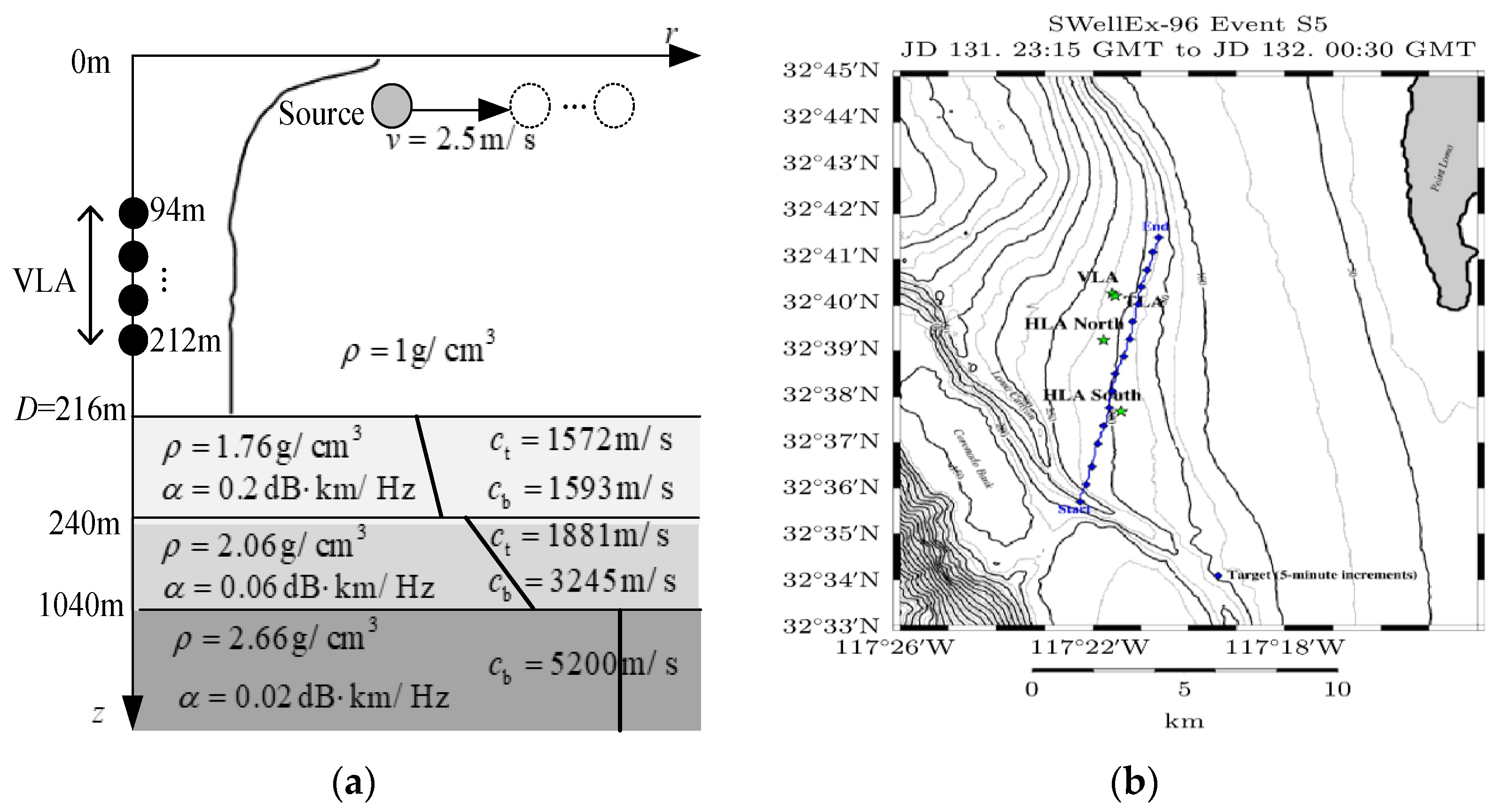
5. SWellEx-96 Experimental Examples

The goal of this section is to investigate PF and PF-S behaviors for the source depth and water depth joint tracking in a layered waveguide with experimental data collected during the SWellEx-96 experiment [30]. Figure 7a includes environmental parameters, such as the thickness (216 m) of a water layer that has sound speed, density, and attenuation, and overlies two sediment layers and a semi-finite basement.

Figure 7b presents a surface ship traveling with a radial velocity of 2.5 m/s towards a 21 element VLA during this experiment; the ship tows a deep (54 m) and a shallow (9 m) source, both projecting different tonal signals. The analyzed data involved two tonal signals, one at 127 Hz that was projected by a shallow source, and the other at 130 Hz and projected by a deep source, both splitting into 232 segments. Acoustic data correspond to source-receiver ranges of 8 km to 7.2 km at the VLA for 6 min.

Due to the fact that there are no perfect boundaries as well as the loss mechanisms present in the ocean waveguide, the energy attenuation of high-order modes is faster than that of low-order modes in received data. We adjust the number of steps to 10, that is, only the first 10 modes are tracked. As the low-order modal propagation angles are small, the angle of the vertical-direction beamforming steering vector is restricted within the interval $\theta \in [0^{°},{60}^{°}]$. This would suppress part of ocean noise. In addition, element values of the state noise covariance matrix are increased by five times to ensure filters with increased convergence speed.

5.1. Convergence Speed

In Figure 8, panels on the left and the right display the 9 m and the 54 m source scenarios separately, including the tracking results of the source depth and water depth parameters by the PF-MAP (stars-marked line) and the PF-S-MAP (triangles-marked line) estimates. The standard deviations of marginal PPDs and marginal smooth PPDs are plotted with different colored shading around the tracking results.

As for tracking results of source depth, Figure 8a shows that the PF-MAP estimates begin to approach the truth in the eighth step, while the PF-S-MAP estimates remain accuracy at each step; both two estimates performed well in Figure 8b. Figure 8a indicates that the PF-MAP converges slowly by comparison with the PF-S-MAP for the 9 m source scenario. This is related to a few important attributes about modal structure in a downward-refracting sound speed environment (see Figure 7a). Amplitudes for the mode spectrum of the shallow source monotonically increase with mode order which, in general, are essentially 0 for the first several modes. Accordingly, the weight of particles at initial tracking steps (low-order modes) has little difference between the one near the truth and the one located in another position. This affects the PF-MAP convergence. In contrast, the PF-S-MAP can effectively reduce the shallow source depth tracking error at initial steps as it uses measurements of all steps, especially for large beam-wavenumber peak amplitudes (correspond to high-order modes).

Figure 8c,d displays that the PF-MAP are not close to true values until the last two steps for tracking results of water depth, while the PF-S-MAP yields good performance at each step. These phenomena are contributed to by the inevitable prior modeling bias in the state equation. If the real values of the state parameters evolve differently from this state evolution model, the PF may be unable to track these changes immediately. For example, the actual environment used here is more complex, with the bias of the assumption for the state equation. Even though the measurement equation may tell the PF that the vertical wavenumber parameter is changing in an unexpected way, the PF may ignore the measurement information if this contradicts the state evolution model. The smoother is the only difference between the PF and the PF-S. This reveals that adding an additional smoothing procedure helps to reduce the impact of state modeling errors.

5.2. Uncertainty Analysis

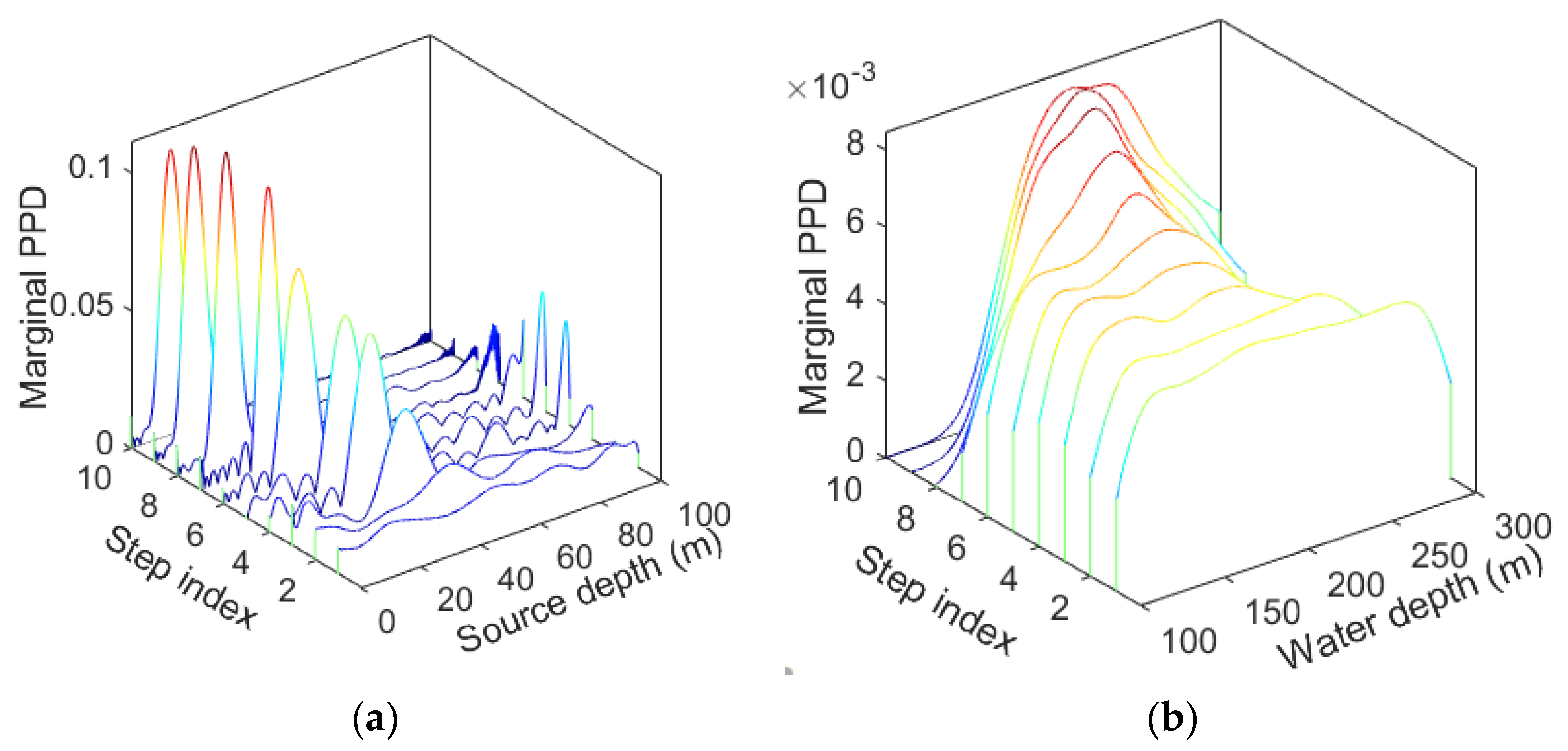
An uncertainty analysis was carried out to assess the advantages of the smoother. We take the 9 m source scenario for the SWellEx-96 Experiment as an example. The evolution of marginal PPDs and marginal smooth PPDs of source depth and water depth parameters at all steps is given in Figure 9a–d.

Marginal PPDs show non-Gaussian, multi-modal distributions with many local probability maxima distributed over the search space in Figure 9a, which indicates unsuccessful tracking of the source depth parameter by the PF. But the marginal smooth PPDs of source depth in Figure 9c correspond to narrow Gaussian PDFs. This shows that the source depth parameter is accurately resolved with small estimation uncertainty by the PF-S. As a comparison with marginal PPDs of the water depth parameter shows a somewhat uniform distribution except for the last few steps in Figure 9b, marginal smooth PPDs are slightly sharper in Figure 9d. Figure 9c,d further shows that the smoother can effectively reduce the uncertainty of source depth and water depth estimation in the joint tracking process.

6. Conclusions

For ocean acoustic applications, there is a natural limit factor with environmental uncertainty. In this paper, a joint tracking approach for source depth and water depth parameters is presented. It might provide a new way to design passive tracking methods in an uncertain shallow-water environment. Our approach establishes the state-space model in the mode domain by exploiting the evolution with mode-order of vertical wavenumber, using particle filtering and the relationship between unknown parameters and beam-wavenumber outputs to obtain tracking results.

The simulation shows that the tracking results of the PF applied in our method are better than the GS. The main reason for this is how the PF utilizes our state-space model while the GS does not. The model includes the evolution of vertical wavenumbers and its inverse relation with water depth, which allows the respective search intervals of prior state parameters to be narrowed. In addition, the recursive filtering (PF) based on the model requires fewer particles than the independent sampling per step pattern (GS) under the premise of the same tracking accuracy, which is beneficial for reducing computational costs. SWellEx-96 experimental results further specify that adding the smoother based on particle filtering is beneficial to reduce uncertainty and tracking errors of source depth and water depth parameters. Because the smoother uses measurements of all steps to correct forward particles’ weights at each step, “tighter” PPDs are generated.

Our approach has practical value in ocean acoustic applications. It enables tracking of source depth and water depth parameters and their underlying uncertainties in shallow water, making the approach a natural extension of target localization and geo-acoustic inversion techniques. The three key advantages of our approach over existing methods are summarized as follows: (1) it does not require any environmental information or numerical calculation from a propagation model and has computational efficiency; (2) it adds an additional smoothing procedure that help to reduce the impact of state modeling errors and effectively reduces the uncertainty of source depth and water depth estimation in the joint tracking process when acoustic field modeling errors exist between our state-space model and the actual waveguide; (3) it has weak sensitivity to ocean noise as observed measurements in our scheme are beam-wavenumber outputs transformed from received data by a vertical line array (VLA) through twice beamforming. This preprocessed step suppresses part of the ocean noise. And the noise immunity of the algorithm will be analyzed in future work.

The depth of a moving source remains constant over a period of time. Nevertheless, the source depth may change over time when a source moves up and down following waves. In this case, we can divide the data over an extended period of time into multiple segments. In each segment time, the source depth is assumed to be constant, and our method is continuously applied to the process. The above scheme in theory also enables our method to be applied to a weakly range-dependent environment where the adiabatic mode approximation can be assumed. Our method is obviously not suitable for the environment with a complicated bottom layer, which should be considered in the follow-up research.

References

- Hinich, M. Tracking a moving vessel from bearing measurements. IEEE J. Ocean. Eng. 1983, 8, 131–135. [Google Scholar] [CrossRef]
- Nardone, S.C.; Graham, M.L. A closed-form solution to bearings-only target motion analysis. IEEE J. Ocean. Eng. 1997, 22, 168–178. [Google Scholar] [CrossRef]
- Rosenqvist, P.A. Passive Doppler-bearing tracking using a pseudo-linear estimator. IEEE J. Ocean. Eng. 1995, 20, 114–118. [Google Scholar] [CrossRef]
- Steele, A.K.; Byrne, C.L.; Riley, J.L.; Swift, M. Performance comparison of high resolution bearing estimation algorithms using simulated and sea test data. IEEE J. Ocean. Eng. 1993, 18, 438–446. [Google Scholar] [CrossRef]
- Dubrovinskaya, E.; Casari, P.; Diamant, R. Bathymetry-aided underwater acoustic localization using a single passive receiver. J. Acoust. Soc. Am. 2019, 146, 4774–4789. [Google Scholar] [CrossRef]
- Nosal, E.M.; Frazer, L.N. Track of a sperm whale from delays between direct and surface-reflected clicks. Appl. Acoust. 2006, 67, 1187–1201. [Google Scholar] [CrossRef]
- Bucker, H. Matched-field tracking in shallow water. J. Acoust. Soc. Am. 1994, 96, 3809–3811. [Google Scholar] [CrossRef]
- Fialkowski, L.T.; Perkins, J.S.; Collins, M.D. Matched-field source tracking by ambiguity surface averaging. J. Acoust. Soc. Am. 2001, 110, 739–746. [Google Scholar] [CrossRef]
- Dosso, S.E.; Nielsen, P.L. Quantifying uncertainty in geoacoustic inversion. II. Application to broadband, shallow-water data. J. Acoust. Soc. Am. 2002, 111, 143–159. [Google Scholar] [CrossRef]
- Tollefsen, D.; Dosso, S.E. Three-dimensional source tracking in an uncertain environment. J. Acoust. Soc. Am. 2009, 125, 2909–2917. [Google Scholar] [CrossRef]
- Dosso, S.E.; Wilmut, M.J.; Nielsen, P.L. Bayesian source tracking via focalization and marginalization in an uncertain Mediterranean Sea environment. J. Acoust. Soc. Am. 2010, 128, 66–74. [Google Scholar] [CrossRef]
- Dosso, S.E. Quantifying uncertainty in geoacoustic inversion. I. A fast Gibbs sampler approach. J. Acoust. Soc. Am. 2002, 111, 129–142. [Google Scholar] [CrossRef] [PubMed]
- Yardim, C.; Michalopoulou, Z.H.; Gerstoft, P. An overview of sequential Bayesian filtering in ocean acoustics. IEEE J. Ocean. Eng. 2011, 36, 71–89. [Google Scholar] [CrossRef]
- Yardim, C.; Gerstoft, P.; Hodgkiss, W.S. Sequential geoacoustic inversion at the continental shelfbreak. J. Acoust. Soc. Am. 2012, 131, 1722–1732. [Google Scholar] [CrossRef] [PubMed]
- Dosso, S.E.; Wilmut, M.J. Uncertainty estimation in simultaneous Bayesian tracking and environmental inversion. J. Acoust. Soc. Am. 2008, 124, 82–97. [Google Scholar] [CrossRef]
- Yardim, C.; Gerstoft, P.; Hodgkiss, W.S. Tracking of geoacoustic parameters using Kalman and particle filters. J. Acoust. Soc. Am. 2009, 125, 746–760. [Google Scholar] [CrossRef]
- Michalopoulou, Z.H.; Yardim, C.; Gerstoft, P. Particle filtering for passive fathometer tracking. J. Acoust. Soc. Am. 2012, 131, EL74–EL80. [Google Scholar] [CrossRef]
- Yardim, C.; Gerstoft, P.; Hodgkiss, W.S. Geoacoustic and source tracking using particle filtering: Experimental results. J. Acoust. Soc. Am. 2010, 128, 75–87. [Google Scholar] [CrossRef]
- Yardim, C.; Gerstoft, P.; Hodgkiss, W.S. Particle smoothers in sequential geoacoustic inversion. J. Acoust. Soc. Am. 2013, 134, 971–981. [Google Scholar] [CrossRef]
- Godsill, S.J.; Doucet, A.; West, M. Monte Carlo smoothing for nonlinear time series. J. Am. Stat. Assoc. 2004, 99, 156–168. [Google Scholar] [CrossRef]
- Besedina, T.N.; Kuznetsov, G.N.; Kuz’kin, V.M.; Pereselkov, S.A.; Prosovetsky, D.Y. Estimation of the depth of a stationary sound source in shallow water. Phys. Wave Phenom. 2015, 23, 292–303. [Google Scholar] [CrossRef]
- Kuznetsov, G.N.; Kuz’kin, V.M.; Pereselkov, S.A.; Prosovetskii, D.Y. Wave Method for Estimating the Sound Source Depth in an Oceanic Waveguide. Acoust. Phys. 2016, 24, 262–281. [Google Scholar] [CrossRef]
- Jensen, F.B.; Kuperman, W.A.; Porter, M.B.; Schmidt, H. Computational Ocean Acoustics, 2nd ed.; Springer: New York, NY, USA, 2011. [Google Scholar]
- Zhou, Y.; Sun, C.; Xie, L. A method of estimating depth of moving sound source in shallow sea based on incoherently matched beam-wavenumber. Acta Phys. Sin. 2023, 72, 084302. [Google Scholar] [CrossRef]
- Yang, T.C. Source depth estimation based on synthetic aperture beamforming for a moving source. J. Acoust. Soc. Am. 2015, 138, 1678–1686. [Google Scholar] [CrossRef]
- Arulampalam, M.S.; Maskell, S.; Gordon, N. A tutorial on particle filters for online nonlinear/non-Gaussian Bayesian tracking. IEEE Trans. Signal Process. 2002, 50, 174–188. [Google Scholar] [CrossRef]
- Kitagawa, G. Monte Carlo filter and smoother for non-Gaussian nonlinear state space models, Journal of Computational and Graphical Statistics. J. Comput. Graph. Stat. 1996, 5, 1–25. [Google Scholar]
- Michalopoulou, Z.H.; Picarelli, M. Gibbs sampling for time-delay-and amplitude estimation in underwater acoustics. J. Acoust. Soc. Am. 2005, 117, 799–808. [Google Scholar] [CrossRef] [PubMed]
- Peter, M.B. The KRAKEN Normal Mode Program; Technical Report; SACLANT Undersea Research Centre: La Spezia, Italy, 1991. [Google Scholar]
- Booth, N.O.; Hodgkiss, W.S.; Ensberg, D.E. SWellEx-96 Experiment Acoustic Data, UC San Diego Library Digital Collections. Available online: http://swellex96.ucsd.edu/ (accessed on 5 July 2023).
Figure 1.
The path sketch of a moving source relative to a VLA.
Figure 2.
The path sketch of a moving source relative to a VLA in an ideal waveguide.
Figure 3.
(a) Beam-wavenumber spectra, where modal horizontal wavenumbers and modal propagation angles are marked by circle symbols and calculated by the KRAKEN program, and cosine transforms between the beam and wavenumber direction are denoted by the dashed line; (b) Beam-wavenumber spectral peaks’ amplitudes, which are obtained by extracting from the positions of circle symbols in (a) to compare with the first 32 modal excitation values (both normalized).
Figure 4.
Tracking results of the GS-MAP (squares-marked line), the PF-MAP (stars-marked line), and the PF-S-MAP (triangles-marked line) in an ideal waveguide: (a) source depth, (b) water depth, and (c) vertical wavenumber. Dashed lines indicate true trajectories.
Figure 5.
RMSE for the GS-MAP (squares-marked line) and the PF-MAP (stars-marked line) at the last 10 tracking steps in terms of (a) source depth and (b) water depth and computed as a function of the number of forward particles.
Figure 6.
RMSE for the PF-MAP (stars-marked line) and the PF-S-MAP (triangles-marked line) at first 10 tracking steps in terms of (top) source depth and (bottom) water depth, computed as a function of the number of backward particles.
Figure 7.
The SWellEx-96 Event S5: (a) The layered waveguide with sound speed profile, VLA, and geo-acoustic parameters; (b) The path of a surface ship in blue towed a deep and a shallow source during the 75 min VLA recording.
Figure 8.
Tracking results of the PF-MAP (stars-marked line) and the PF-S-MAP (triangles-marked line) for the SWellEx-96 experiment in the 9 m (left panels) and 54 m (right panels) moving source scenario: (a,c) source depth; (b,d) water depth. Dashed lines indicate true trajectories.
Figure 9.
Evolving marginal PPDs (top panels) and marginal smooth PPDs (bottom panels) at all steps in the 9 m source scenario for the SWellEx-96 experiment: (a,c) source depth; (b,d) water depth. Illustrating parameters uncertainty.