Real-Time Underwater Acoustic Homing Weapon Target Recognition Based on a Stacking Technique of Ensemble Learning

Abstract

Underwater acoustic homing weapons (UAHWs) are formidable underwater weapons with the capability to detect, identify, and rapidly engage targets. Swift and precise target identification is crucial for the successful engagement of targets via UAHWs. This study presents a real-time target recognition method for UAHWs based on stacking ensemble technology. UAHWs emit active broadband detection signals that manifest distinct reflection characteristics on the target. Consequently, we have extracted energy and spatial distribution features from the target’s broadband correlation detection output. To address the problem of imbalanced original sea trial data, we employed the SMOTE algorithm to generate a relatively balanced dataset. Then, we established a stacking ensemble model and performed training and testing on both the original dataset and relatively balanced dataset separately. In conclusion, we deployed the stacking ensemble model on an embedded system. The proposed method was validated using real underwater acoustic homing weapon sea trial data. The experiment utilized 5-fold cross-validation. The results indicate that the method presented in this study achieved an average accuracy of 93.3%, surpassing that of individual classifiers. The model’s single-cycle inference time was 15 ms, meeting real-time requirements.

1. Introduction

When underwater acoustic homing weapons (UAHWs) employ active sonar for detecting, locating, tracking, and targeting submarines, they encounter the challenge of dealing with a variety of acoustic decoys deployed by the submarines to mislead them. To ensure the successful targeting of submarines, UAHWs must be equipped with active target recognition capabilities. This enables them to effectively identify submarines and counter various acoustic decoys. Scholars have undertaken research on real and decoy target recognition technology for UAHWs. According to [1], the essential principle behind real and decoy target recognition technology for active acoustic homing is the differentiation of real targets from “decoy targets” generated by underwater acoustic countermeasures based on their scale characteristics. Hence, scale characteristics play a pivotal role in the initial target recognition process of underwater acoustic homing weapons. Early researchers successfully accomplished scale target recognition by employing the azimuth analysis method [2,3]. Nevertheless, as underwater acoustic countermeasures have advanced, acoustic decoys have transitioned from point source decoys to scale decoys equipped with extensive towed arrays. This evolution has rendered it unfeasible to distinguish scale decoys from submarines solely based on scale features [4,5]. Consequently, there is an urgent imperative to develop a target recognition method for scale decoys in UAHWs.

In recent years, the rapid advancement of artificial intelligence (AI) has provided new avenues for target recognition. Conducting research on intelligent acoustic target recognition holds significant practical importance. Currently, AI and machine learning technologies have been widely applied to acoustic target recognition issues [6,7]. Underwater acoustic target recognition methods based on AI can be divided into statistical machine learning methods and deep learning methods. Among them, the object recognition method based on statistical machine learning includes support vector machine [8,9] and other methods [10], while the object recognition method based on deep learning includes convolutional neural networks [11,12,13,14,15], long short-term memory [16], and other methods [17]. It can be observed that for passive underwater acoustic target recognition, scholars have conducted a substantial amount of research. However, there has been relatively less research on active target recognition methods based on AI. Due to its ability to efficiently address various real-world problems, ensemble learning has garnered significant attention in the field of machine learning, and the stacking ensemble technique is an important method within ensemble learning. Stacking ensemble learning can integrate the strengths of various traditional machine learning methods, exhibiting strong generalization abilities with minimal impact on time and space complexity. Therefore, stacking ensemble learning is well suited for applications in scenarios with high real-time requirements. Currently, the stacking ensemble technique has been applied in various fields, including rainfall prediction [18], ocean wave height prediction [19], rock mass classification [20], and damage prediction [21].

In this study, we presented a real-time target recognition method for UAHWs based on the stacking ensemble technique. It was designed to address the issue of identifying submarines and scale decoys in UAHWs. Firstly, under the active wideband detection waveform illumination of UAHWs, submarines exhibited the characteristic of multi-highlight surface reflection, while scale decoys exhibited the characteristic of multi-highlight point reflection. From the output of target broadband signal correlation detection, we extracted statistical features of target echo energy distribution and spatial distribution. Next, we constructed a stacking ensemble model suitable for UAHWs. In addition to the stacking ensemble model, we established seven other classifiers, including SVM, KNN, LR, DT, GBDT, and XGBoost, for comparison with the stacking ensemble model. Then, addressing the issue of imbalanced data in the available real-world data, we employed the SMOTE oversampling method to obtain a relatively balanced dataset. With both the imbalanced and balanced datasets, we separately trained and tested the stacking ensemble model and the seven individual classifiers. We analyzed the advantages of the stacking ensemble model over individual classifiers and discussed the impact of imbalanced datasets on classifier prediction performance. Finally, we deployed the stacking ensemble model on an embedded system and calculated the inference time.

The structure of this study is as follows: Section 2 introduces the fundamental principles and methods; Section 3 presents the recognition method workflow; Section 4 provides the prediction results and analysis and outlines the process and results of deploying the model on an embedded system; Section 5 presents the discussion; and Section 6 presents the conclusions.

2. Materials and Methods

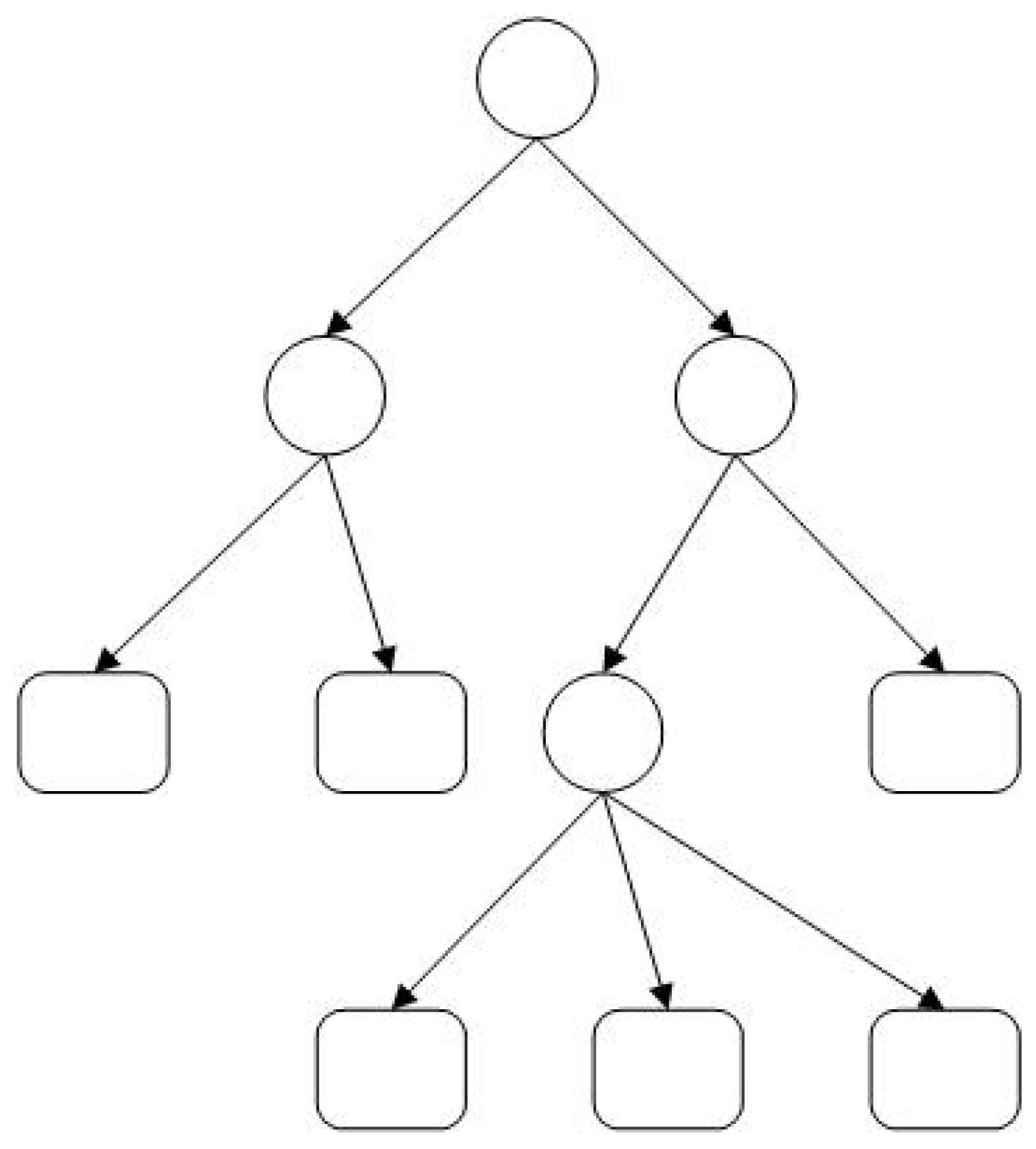
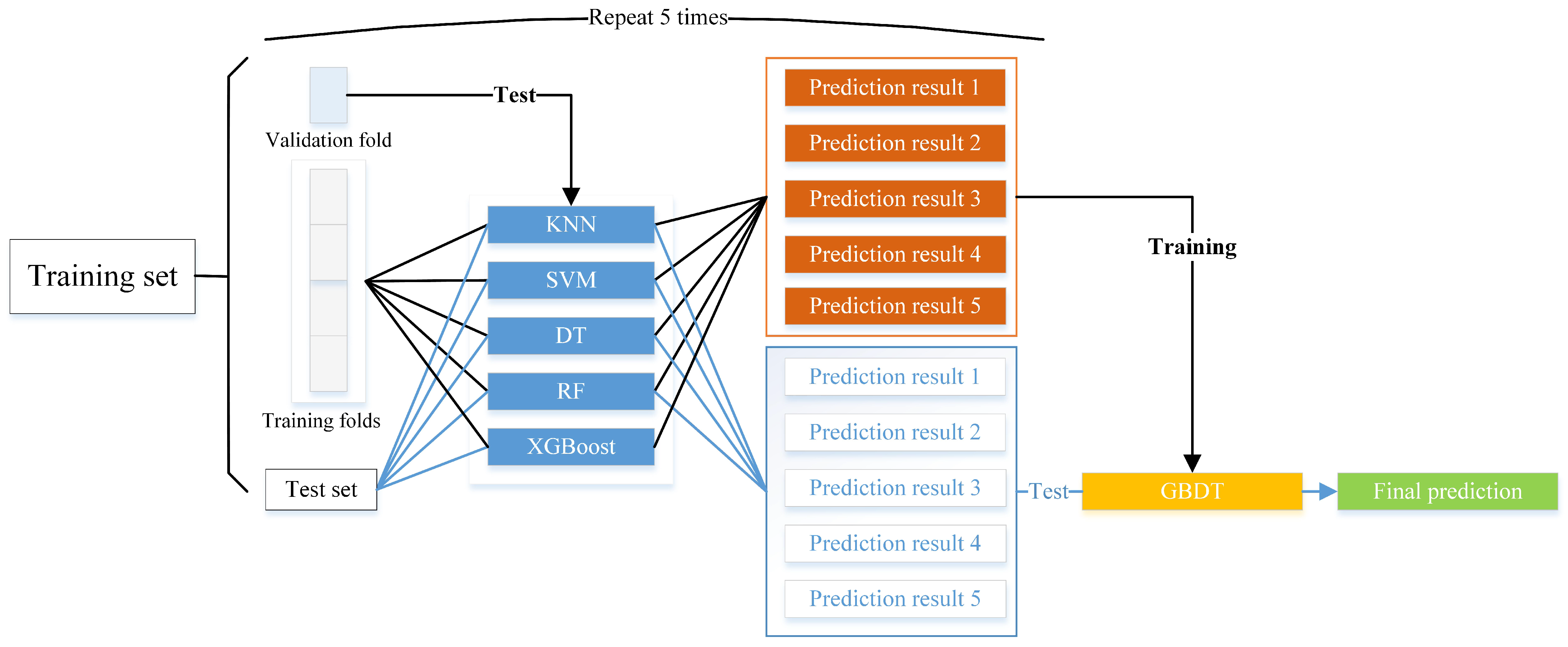
2.1. Stacking Ensemble Learning

Ensemble learning is a technique that involves the combination of multiple models to make predictions, aiming to achieve more accurate and robust results compared to those of a single classification model. Ensemble learning typically falls into three categories: boosting, bagging, and stacking. In boosting and bagging, the same base classifier is utilized, making them homogeneous ensemble methods. In contrast, stacking [22] employs various types of base learners for integration, earning it the designation of a heterogeneous integration method. In order to integrate multiple classification models, a stacking ensemble model first divides the original dataset into several sub-datasets. Then, each classification model is considered as a base model, and their prediction results for the data are output as meta-features of the data. Finally, the meta-model is trained using the previously extracted meta-features to make the final predictions. To avoid overfitting, we used k-fold cross-validation to partition the dataset before training multiple heterogeneous models. Our approach is rooted in our decision not to assign explicit weight coefficients to individual base models. Instead, we harness the predictions generated by these base models. This approach empowers the meta-model to correct discrepancies in the predictions made by the base models, effectively reducing the risk of overfitting. Therefore, our model is a “two-layer” ensemble model, rather than a “weighted” model. The following are the steps to establish a “two-layer” stacking ensemble model:

• The dataset $S=[(x_i,y_i),i=1,...,N]$ is divided into a training set $S_{train}=[(x_{tr},y_{tr}),$$tr=1,...,N_{train}]$ and a test set $S_{test}=[(x_{te},y_{te}),te=1,...,N_{test}]$. In these sets, $x_i$ represents the i-th sample in the dataset, and $y_i$ corresponds to the class of the i-th sample. For the training set, $x_{tr}$ represents the $tr$-th sample, and $y_{tr}$ is the class associated with the $tr$-th sample. In the test set, $x_{te}$ represents the $te$-th sample, and $y_{te}$ is the class associated with the $te$-th sample.
• k base classifiers are selected, and the training set $S_{train}$ is divided into k equal size subsets $S_1,S_2,...,S_k$. Define $S_{-k}$ as a test set; then, $S_{\ast k}=S-S_k$. All k base models are trained using the training set $S_{train}$, and prediction probabilities $z_{k,p}$ are obtained using the test set. A new training set is obtained by combining the predicted probabilities of each base model on the test set during cross-validation. At the same time, the predicted probabilities of each base model on the total test set are averaged, and a new test set is obtained after concatenation.
• The second level meta-model is trained with the newly generated training set. By training the meta-model, the prediction deviation of the base model can be corrected and the prediction accuracy can be improved.

2.2. Base Classifiers

Selecting base classifiers and meta-classifiers plays a vital role in establishing stacking ensemble classifiers. In order to select the appropriate base and meta-classifiers and compare them with stacking ensemble classifiers, we established seven commonly used classifiers, including support vector machine, k-nearest neighbors, decision tree, logistic regression, random forest, gradient boosting decision trees, and extreme gradient boosting decision trees. The following provides a brief introduction to each classifier.

2.2.1. Support Vector Machine

Support vector machine (SVM) is a supervised learning method, which can be widely used in statistical classification and regression analysis [23]. By mapping data points to high-dimensional space, a segmentation hyperplane is found in high-dimensional space. The segmentation hyperplane is determined by weighing the minimum interval and error rate. The interval refers to the distance from the segmentation hyperplane to the support vector, and the error rate refers to the number of incorrectly classified objects. At the same time, kernel functions are used to map data points to high-dimensional spaces, thereby reducing the difficulty of classification. For the binary classification problem in this study, assuming a training set is $(x_i,y_i)(i=1,2,...n,y\in [-1,1])$, a hyperplane can be constructed as $wx+b=0$, where w is the normal vector determining the direction of the hyperplane, and b is the offset term determining the distance between the hyperplane and the origin. The solution to the hyperplane is a constrained optimization problem, and by utilizing the Lagrange multiplier duality, it can be transformed into the following optimization problem:

$$\begin{array}{c}\underset{\alpha }{max}[\sum _{i=1}^n{\alpha }_i-\frac{1}{2}\sum _{i=1}^n\sum _{j=1}^n\left({\alpha }_i{\alpha }_j{y}_i{y}_j\right)]\\ \mathrm{s}.t.\sum _{i=1}^n({\alpha }_i{y}_i=0)(0<{\alpha }_i<C,i=1,2,...,n)\end{array}$$

(1)

where ${\alpha }_i$, ${\alpha }_j$ represents the Lagrange multiplier, and C is the penalty coefficient. The ultimate optimal classification function is given by:

$$f\left(x\right)=sgn\left[\sum _{i=1}^n({\alpha }_i^{\ast }{y}_i{x}_i{x}_i^T+b^{\ast })\right]$$

(2)

where ${\alpha }_i$ represents the optimal Lagrange multiplier, and $b^{\ast }$ is the optimal coefficient b. Moreover, given the nonlinear nature of the problem in this study, we incorporated a radial basis kernel function, expressed as follows:

$$k(x_i,x_j)=exp(-\frac{1}{2{\gamma }^2}{∥x_i-x_j∥}^2)$$

(3)

where $\gamma$ represents the bandwidth of the radial basis kernel function.

2.2.2. k-Nearest Neighbors

k -nearest neighbor (KNN) [24] is a lazy learning classifier. The main idea is to calculate the distance between the test samples and the samples in the training set. According to the hyperparameter k preset in KNN, the nearest k samples in the training set determine the type of test sample. KNN is simple in principle, without preconditions and assumptions, it has a wide range of applications, and it is less affected by outliers. Its drawbacks include high computational complexity, high storage space requirements, and susceptibility to imbalanced data. Assuming $x_q^t$ is the feature vector to be classified, KNN entails seeking the most similar feature vectors within the sample space. Following this, a vote is cast among the k-nearest vectors, and the class with the highest frequency is assigned to the target vector. Euclidean distance serves as the metric for measuring vector similarity and can be expressed as:

$$D_E=\sqrt{\sum _{q=1}^d{(x_q^s-x_q^t)}^2}$$

(4)

where $D_E$ is the Euclidean distance, $x_q^s$ is the sample vector, and d is the dimensionality of the sample.

2.2.3. Decision Tree

As depicted in Figure 1, decision tree (DT) [25] is a type of decision making, based on a tree structure, that classifies a dataset through multiple conditional discriminant processes and ultimately obtains the desired results. The CART decision tree is used in this study, using the Gini coefficient as the basis for partitioning. The advantage is that the nonparametric model does not require pre-assumptions about the samples and can handle complex samples. Its calculation speed is fast, the interpretability of the results is strong, and it is not sensitive to missing values. In the tree structure, each internal node represents a judgment on an attribute, each branch represents an output of a judgment result, and, finally, each leaf node represents a classification result. For a classification problem with K classes, where the probability of a sample belonging to the k-th class is $p_k$, the Gini index for the probability distribution can be defined as:

$$Gini\left(p\right)=\sum _{k=1}^K{p}_k(1-p_k)=1-\sum _{k=1}^K{p}_k^2$$

(5)

2.2.4. Logistic Regression

Logistic regression (LR) [26] assumes that the data obey the Bernoulli distribution and performs classification using the method of maximizing the likelihood function to solve the parameters via gradient descent. The advantage is that the classification possibility is directly modeled, avoiding the problems caused by inaccurate distribution assumptions. It is easy to use, with strong interpretability. However, LR is prone to underfitting and has relatively poor classification accuracy. When the feature space is large, the performance is relatively poor. The logistic regression model can be expressed as:

$$\begin{array}{c}\hfill P(y=1|x)=\frac{exp(w·x+b)}{1+exp(w·x)+b}\\ \hfill P(y=0|x)=\frac{1}{1+exp(w·x)+b}\end{array}$$

(6)

where x represents the input features, y is the output class, w is the weight vector, b is the bias term, and $w·x$ denotes the dot product of w and x.

Figure 1. Decision tree model.

Figure 1. Decision tree model.

2.2.5. Random Forest

Random forest (RF) is an ensemble classifier based on DTs [27]. It uses the bootstrap resampling technique repeatedly to extract n different samples from the original dataset to create a new training sample set to train the decision trees and then generates n decision tree classifiers. Each decision tree classifier predicts the test samples and integrates n generated decision trees using the bagging method. Here are the main steps of Random forest:

• Data Sampling (Bootstrap): For a given training dataset, a random forest performs random sampling with replacement, generating multiple different subsets. This is referred to as bootstrap sampling. This means that certain samples may appear multiple times in one subset, while others may not appear at all.
• Feature Random Selection: At each node of every decision tree, a random forest does not consider all features for splitting; instead, it randomly selects a subset of features from the feature set. This helps increase the diversity of the model and prevents overfitting.
• Decision Tree Training: For each bootstrap-sampled subset and feature subset, a decision tree is trained. The commonly used decision tree algorithm is CART (Classification and Regression Trees).
• Voting or Averaging: For classification problems, a random forest employs a majority voting approach, where each decision tree votes for a class, and the final prediction is the class with the most votes.

Ultimately, the output of a random forest can be expressed as:

$$y=majorityvote(f_1\left(x\right),f_2\left(x\right),...,f_n\left(x\right))$$

(7)

where y is the prediction of the random forest, and $f_i\left(x\right)$ is the prediction of the i-th decision tree.

2.2.6. Gradient Boosting Decision Tree

Gradient boosting decision tree (GBDT) [28] is an ensemble classifier based on DTs. In each iteration, a new DT is generated, and the residual of the previous DT is used to train the current DT. In addition, in each iteration, the gradient descent method is used to increase the weight of misclassified samples so that the objective function error of the model is smaller than the previous iteration. The convergence condition of this algorithm is to meet the preset classification error or reach the upper limit of the DT. Finally, all trained DTs are integrated into one classifier. GBDT has strong generalization ability and is widely used in classification problems.

2.2.7. Extreme Gradient Boosting Decision Tree

Extreme gradient boosting decision tree (XGBoost) [27,29] is a large-scale parallel lifting tree algorithm. Similar to GBDT, it also adopts the boosting method, but its objective function is different from GBDT. This method is fast and can perform parallel calculations.

2.3. SMOTE

Synthetic minority oversampling technique (SMOTE) [29,30] is a data processing method employed to address imbalanced datasets. The SMOTE algorithm harnesses the KNN model from the realm of machine learning to generate new samples. This approach distinguishes itself from the simple replication of minority class samples commonly utilized in basic random oversampling. In contrast to random oversampling techniques, SMOTE effectively mitigates the overfitting issues associated with such methods. The fundamental principle of the SMOTE algorithm is as follows: Initially, it selects minority class samples to create new synthetic samples, drawing from the minority class. It then traverses through all the minority class samples. Subsequently, a sample is randomly chosen from all the samples within the k-nearest neighbors of the sample slated for oversampling. Linear interpolation is employed in accordance with Formula (1) to create the synthetic new sample.

$$x_{new}=x_i+rand(0,1)\ast ∥{\widehat{x}}_i-x_i∥$$

(8)

where $rand(0,1)$ represents a random value between 0 and 1, ${\widehat{x}}_i$ denotes a randomly selected sample from the k samples, $x_i$ denotes the sample to be oversampled, and $x_{new}$ represents the newly synthesized sample.

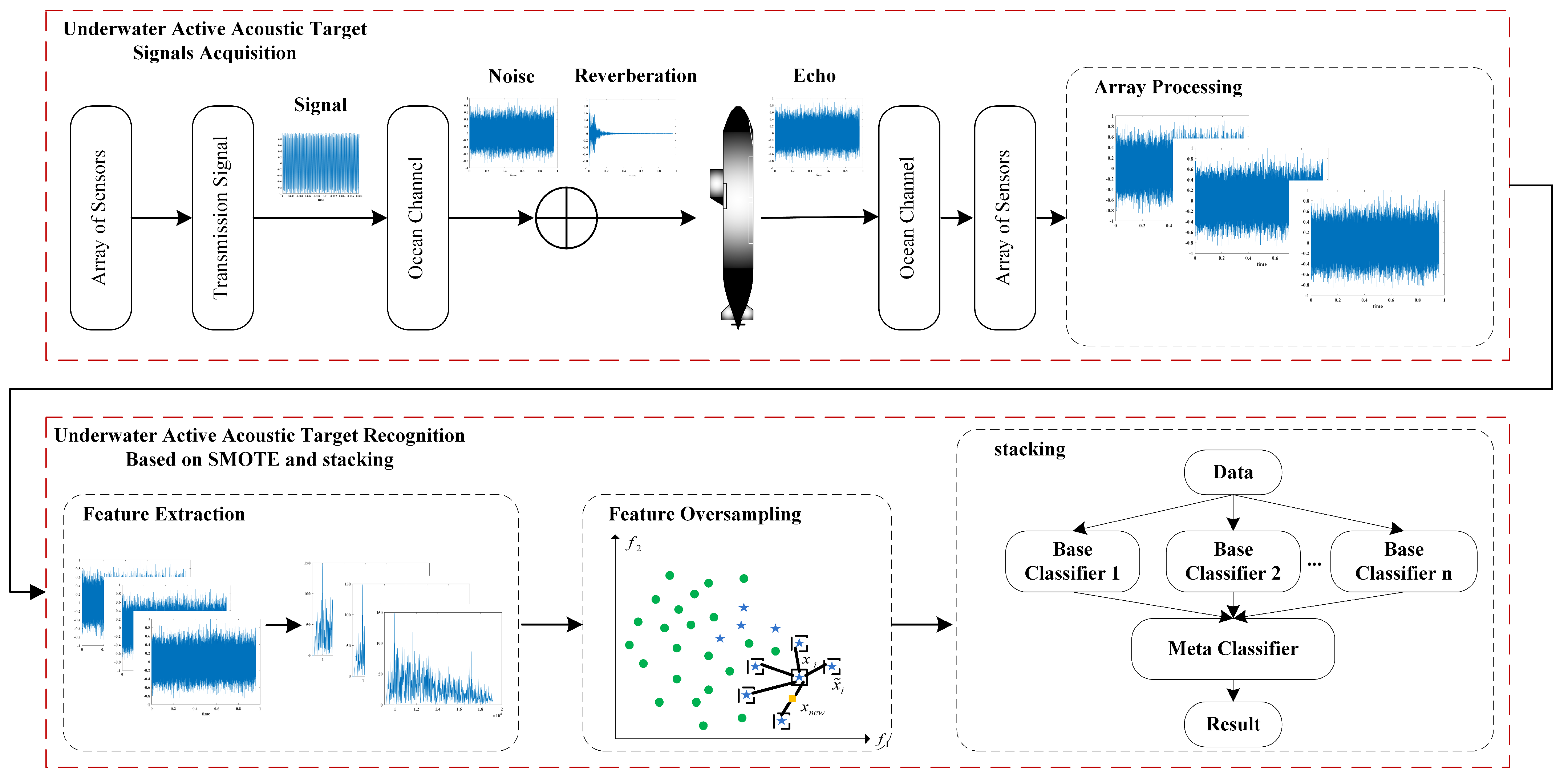
3. Modeling of UAHW Target Recognition Algorithm Based on SMOTE-Stacking

UAHWs employ active sonar for target detection. Initially, UAHWs utilize their array of sensors to emit frequency-modulated signals, which propagate through the ocean channel, reach the target, and reflect as echoes. These target echoes, after transmission through the ocean channel, are received by the sensor array of UAHWs and undergo array signal processing and correlation detection. In addition to interference from marine environmental noise, they are also influenced via reverberation. After receiving the target echoes through the sensor array, UAHWs initiate beamforming to achieve spatial filtering. Subsequently, the signal, post-beamforming, undergoes correlation detection. To mitigate the impact of reverberation, a time-varying gain control method is applied. Following correlation detection, the highlights corresponding to the target echoes are obtained. Feature extraction is then conducted based on these highlights. Due to a significant disparity in the quantity of submarine target echoes compared to decoy target echoes in the dataset, SMOTE is employed in the feature domain. Ultimately, target recognition is accomplished through the utilization of the stacking ensemble method. An entire workflow of the target recognition algorithm is depicted in Figure 2.

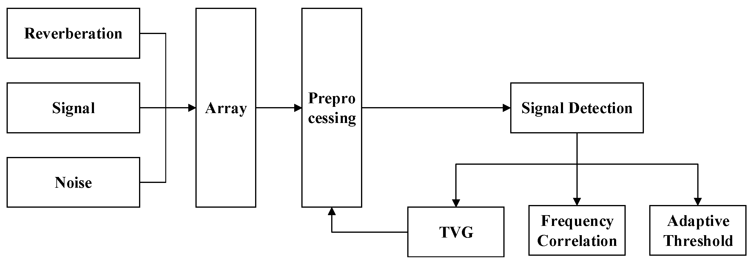
3.1. Active Acoustic Signal Detection System of UAHW

The UAHW uses an active acoustic sonar system to detect, locate, and track targets. In active sonar systems, the emission signal is known. If the additive noise is white Gaussian, the best detector given by the likelihood ratio test is a cross-correlator or matched filter. The detection background consists of marine environmental noise, self-noise, circuit noise, and reverberation. To reduce noise and reverberation interferences as much as possible, we adopt beamforming before detection and the time-varying gain control (TVG) method, respectively. A typical active sonar signal processing structure is shown in Figure 3.

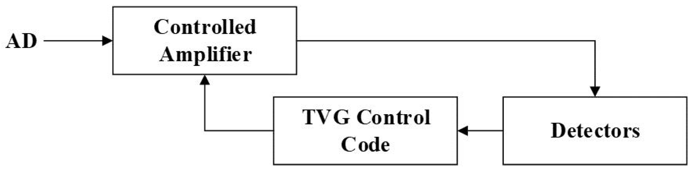
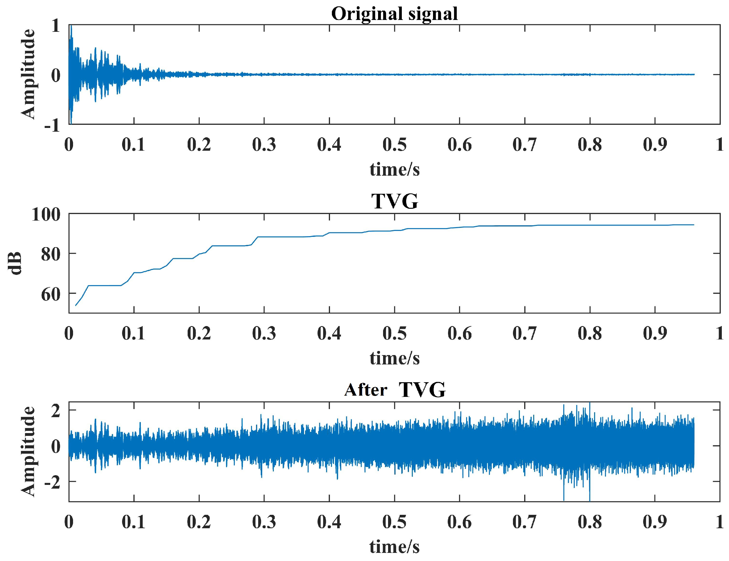
3.1.1. Time-Varying Gain Control (TVG)

In active acoustic sonar systems, the echo signal from the target is submerged in the reverberation and noise background. Reverberation is a non-stationary stochastic process with time-varying amplitude, frequency, air variation, and color. The target radiation noise and target echo received by UAHWs continuously strengthen as they approach the target. In order to keep the reverberation, echo, and target radiation noise within the effective dynamic range of the receiver and within the voltage range that the A/D converter can operate correctly, the constant false alarm processing of homing signal detection first needs to solve dynamic range compression and background normalization.

We adopt time-varying gain control (TVG) for dynamic range compression. Its processing flow is shown in Figure 4. The detector detects and integrates the output of the receiver, forming a control code for the controlled amplifier, thereby changing the amplifier gain. TVG can effectively implement dynamic range compression. However, due to the non-stationary nature of the background, its normalization of the background cannot achieve constant variance. As shown in Figure 5 and Figure 6, the original signal, TVG gain curve, and the signal processed via TVG are presented. It can be seen that after TVG, the reverberation, echo, and target radiation noise are all within the effective dynamic range of the receiver.

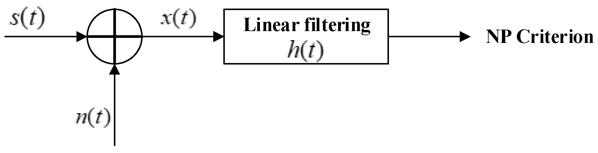
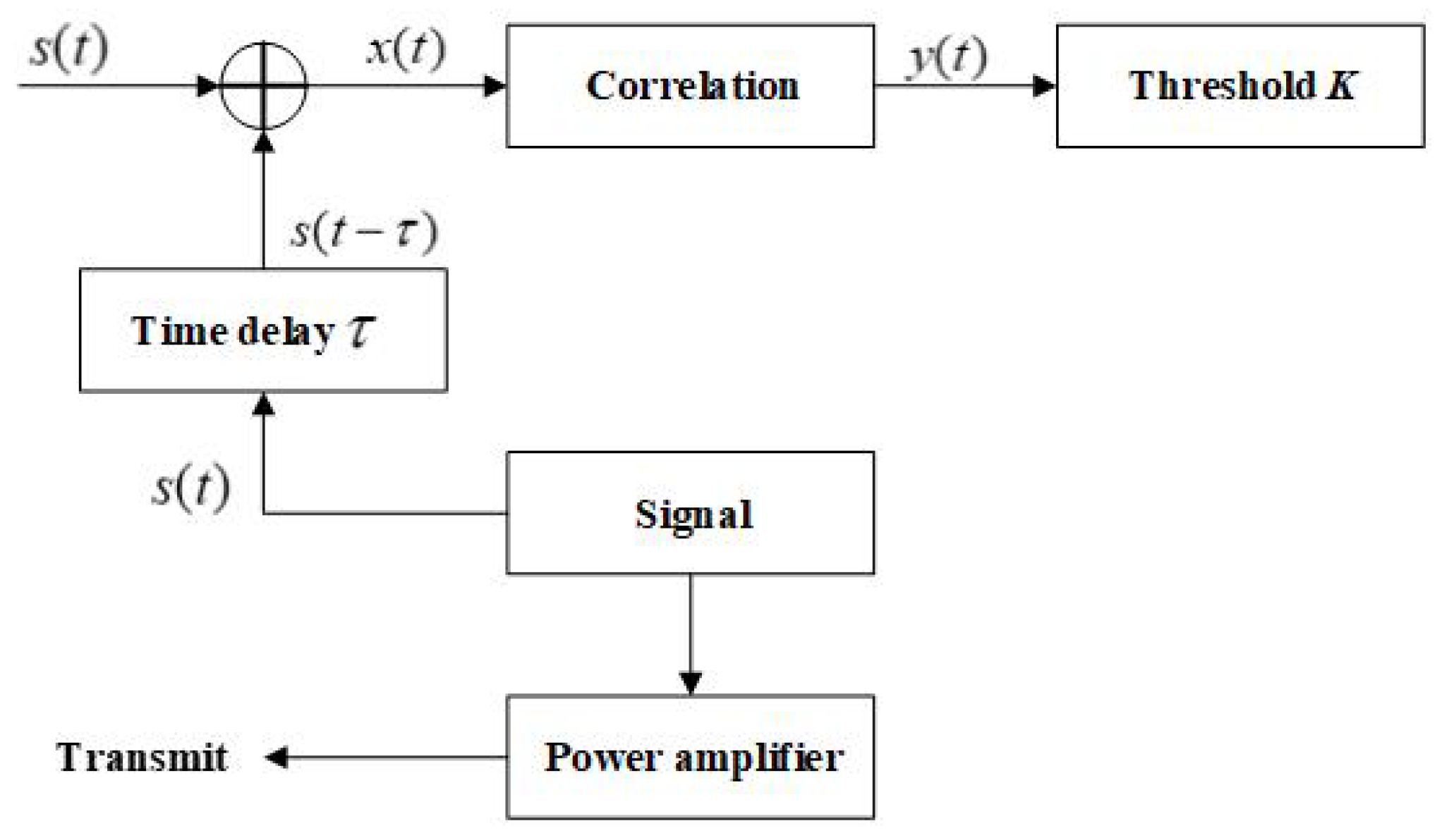
3.1.2. Adaptive Threshold

The purpose of signal detection is to extract as many useful signals as possible from noise-polluted signals. For signal detection, there are two hypotheses: $H_0$ contains no signal and $H_1$ contains a signal, which can be expressed as:

$$H_0=n\left(t\right)H_1=s\left(t\right)+n\left(t\right)$$

(9)

where $s\left(t\right)$ and $n\left(t\right)$ are the signal and noise, respectively.

The detection system requires the best criterion to be met under the given assumptions. For active sonar systems, the optimal detection is typically based on the Neiman–Pearson criterion, and the likelihood ratio is calculated via a matched filter. A matched filter is an optimal linear filter. When the input signal is known, and the background noise is white noise, then the output SNR of the matched filter reaches its maximum. The optimal detection system of active sonar can be simplified as the structure presented in Figure 7. In fact, the matched filter was implemented through the cross-correlation. As presented in Figure 8, the input signal is $s\left(t\right)$ and the background noise is $n\left(t\right)$. Assume that $n\left(t\right)$ is white noise, and its power spectrum density is $\frac{N_0}{2}$. Then, the max output SNR of the matched filter is $\frac{2E}{N_0}$, where E is the energy of $s\left(t\right)$.

TVG can effectively implement dynamic range compression. However, due to the non-stationary characteristics of the background, their normalization of the background can not reach constant variance. Another important measure to achieve constant false alarm processing is adaptive threshold processing. The calculation of adaptive thresholds is closely related to the signal form and signal processing methods used in homing. Dynamic compression, background normalization, and adaptive thresholds constitute constant false alarm processing for homing signal detection. Adaptive threshold processing is the ability to adaptively adjust the detection threshold as the interference background changes, thereby enabling more accurate detection of targets. We adopt an adaptive threshold generation method based on low-pass filters. This adaptive threshold generation method assumes that after low-pass filtering, the relevant peaks of the signal will be filtered out. Therefore, the design of low-pass filters is crucial and must be determined based on the shape of the signal’s relevant peaks. In addition, when generating the detection threshold in the final step, a fixed offset can be added to the entire threshold as needed, which should be related to the current background.

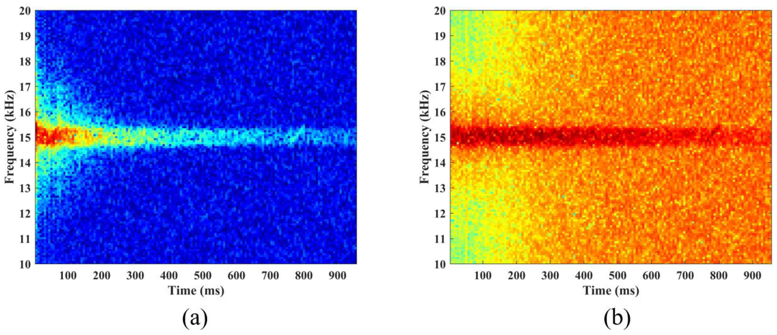
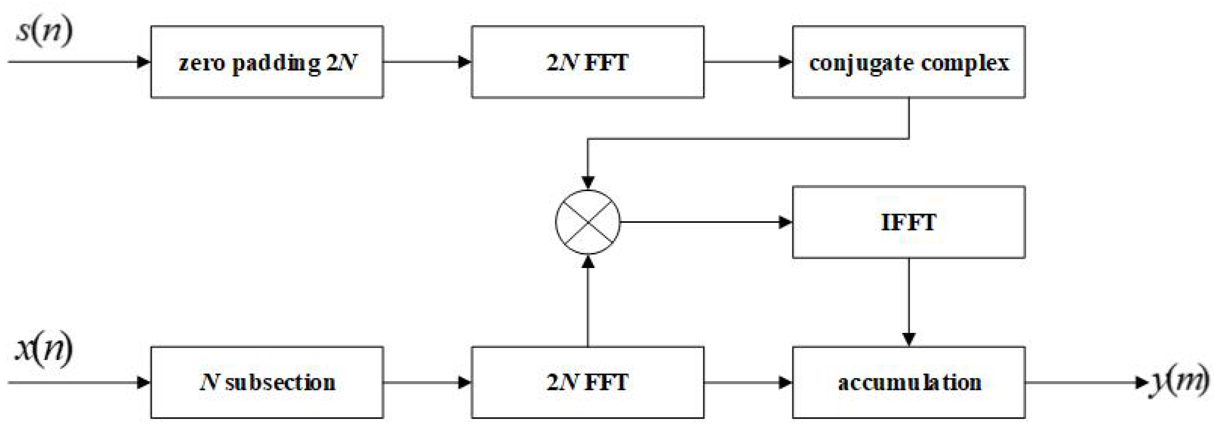
3.1.3. Frequency Correlation

In order to achieve fast correlation detection, frequency-domain correlation is used for signal detectors. As presented in Figure 9, frequency-domain correlation uses cyclic convolution, fast Fourier transform ($FFT$), and inverse fast Fourier transform ($IFFT$) for signal detection. The detection algorithm can be defined using the following:

$$y_m(n,v)=abs\left(IFFT[FFT\left(x_m\left(n\right)\right)\ast {\left(FFT\left(s_v\left(n\right)\right)\right)}^{\prime }]\right)$$

(10)

where $x_m\left(n\right)$ and $s_v\left(n\right)$ denote the received and reference signals, respectively.

3.2. Feature Extraction

After signal detection, feature extraction is performed. The extraction of effective features is a crucial step when building a model, and the quality of features plays a decisive role in the prediction process. The linear array scale acoustic decoy has the characteristics of highlight and azimuth extension, and it responds to the detection signal regularly through multiple underwater acoustic transducers. When the response signals of multiple underwater acoustic transducers are superimposed, the azimuth strike characteristics and multi-highlight characteristics of submarine targets can be simulated with high fidelity. The typical characteristics of the scale acoustic decoy response signal are its stable intensity distribution and spatial distribution, and the background between the highlights is “clean” [4]. The linear array scale acoustic decoy can not only simulate the reflection characteristics of the target to the wideband incident signal and the radiated noise characteristics of the real target but also simulate the scale characteristics of the real extended target physical structure and the spatial distribution characteristics of the echo signal. Compared with the stable highlight of linear array scale acoustic decoys, submarine echoes also have the characteristics of multi-highlight [31]. Due to the irregular shape of submarines, the intensity distribution and spatial distribution of echo bright spots are not the same at different angles, which is a kind of surface reflection. Its highlight background is not clean because of surface reflection. Based on the physical mechanism of the multi-point reflection and submarine surface reflection of linear array scale acoustic decoys, we extracted target-based energy features from the wideband signal correlation detection output, including five features: single highlight energy distribution features, multi-highlight energy distribution features, multi-highlight background energy distribution features, multi-highlight global spatial distribution features, and multi-highlight local spatial distribution features. This feature set can be used to identify submarine and linear array scale acoustic decoys.

3.3. Feature Oversampling Based on SMOTE

The data for this study were obtained from multiple sea trials conducted using UAHWs. The data quantities are presented in

Table 1. Data source and quantity description.

Target Type	Sea Trial Number	Data Number
Acoustic decoy	10	349
Submarine	50	889

. Specifically, the acoustic decoy dataset comprises 349 data samples collected from 10 different sea trials, while the submarine dataset comprises 889 samples from 50 distinct sea trials.

As shown in Table 1, it is clear that the sea trial data display an imbalance in the quantity of the two target classes. For ease of representation, both target types were encoded, with 0 representing acoustic decoys and 1 representing submarines. To prevent information leakage and in consideration of the operational characteristics of UAHWs, we implemented a 5-fold cross-validation with data stratification. For each training dataset in the 5-fold cross-validation, the ratios of acoustic decoy samples to submarine samples in both the training and test datasets are 287/731, 295/714, 289/701, 276/701, and 249/709, which are approximately 2/5, 2/5, 2/5, 2/5, and 1/3, respectively. To analyze the impact of imbalanced data on our algorithm, we performed oversampling, using SMOTE, on the features extracted from the original data. It is crucial to emphasize that this oversampling was exclusively applied to the training set. We doubled the number of acoustic decoy features in the training set while keeping the number of submarine features unchanged. During this process, the k in the SMOTE algorithm was set to 5. The t-SNE [32] visualization results for the original 5-fold cross-validation of features are presented in Figure 10. Figure 11 illustrates the corresponding t-SNE visualization results for the 5-fold cross-validation after oversampling.

3.4. Model Establishment

The problem of target recognition for underwater homing weapons is a few-shot recognition problem. SVM exhibits outstanding performance and is well-suited for small-sample scenarios. KNN is easy to implement and also suitable for small-sample problems. DTs offer good interpretability, which is crucial for underwater homing weapons. RFs provide high accuracy and robustness, while XGBoost excels in performance and scalability, making it highly versatile. And, in the first layer of the stacking ensemble model, we selected five different learners, specifically KNN, SVM, DT, RF, and XGBoost. The meta-classification model chosen was GBDT. To enhance the model’s robustness, we conducted 5-fold cross-validation on the training set. In each training and testing iteration, the data were divided into five parts, with four parts used for training the model, and one part used as a validation set for model evaluation. For instance, in one training and testing iteration, these four data segments were employed as inputs for the first layer of the stacking model, incorporating the five different learners, resulting in five predictions. These five predictions were subsequently used as inputs for the second-layer meta-learner and were utilized for training. A validation dataset was employed as model input for testing in order to search for the optimal hyperparameters. As illustrated in Figure 12, the entire training and testing process was repeated five times to cover all the training data.

Figure 11. The t-SNE visualization results for the 5-fold cross-validation of features after SMOTE oversampling.

Figure 11. The t-SNE visualization results for the 5-fold cross-validation of features after SMOTE oversampling.

4. Results and Analysis

4.1. Evaluation Metrics

To evaluate the predictive performance of our model, we utilized a range of evaluation metrics to assess the performance of the machine-learning-based models. Considering the data imbalance, six evaluation metrics were employed: accuracy ($acc$), area under the receiver operating characteristic curve ($AUC$), F1 score ($F1$), precision ($PRE$), recall ($REC$), and the kappa coefficient ($kappa$).

Table 2. Two-class confusion matrix.

	Predicted Positive	Predicted Negative
Actual positives	TPs (true positives)	FNs (false negatives)
Actual negatives	FPs (false positives)	TNs (true negatives)

represents a confusion matrix for the binary target recognition problem. In the table, $TP$ refers to the number of samples belonging to the positive class and correctly predicted as positive-class samples by a classifier. $FN$ indicates the number of samples from the positive class that are incorrectly predicted as negative-class samples. $FP$ represents the number of samples from the negative class that are incorrectly predicted as positive-class samples. Lastly, $TN$ signifies the number of samples from the negative class that are correctly predicted as negative-class samples.

The evaluation metrics can be calculated based on a confusion matrix, and the corresponding calculation formulae are as follows:

$$acc=\frac{TP+TN}{TP+TN+FP+FN}$$

(11)

$$PRE=\frac{TP}{TP+FP}, REC=\frac{TP}{TP+FN}$$

(12)

$$F1=\frac{2\times PRE\times REC}{PRE+REC}$$

(13)

$$kappa=\frac{p_0-p_e}{1-p_e}$$

(14)

$$p_0=\frac{TP+TN}{TP+TN+FP+FN}$$

(15)

$$p_e=\frac{(TP+FP)\times (TP+FN)+(TN+FN)\times (TN+FP)}{{(TP+TN+FP+FN)}^2}$$

(16)

The form of the ROC curve is also a metric that can be used to evaluate the prediction accuracy of classifiers. The ROC curve plots the true positive rate (TPR, i.e., recall) versus the false positive rate (FRP = FP/(TN + FN)). $AUC$ is referred to as the area under the ROC curve. The $AUC$ values vary from 0.5 to 1, indicating the discrimination accuracy, which can be divided into five categories: no discrimination (0.5–0.6), poor discrimination (0.6–0.7), fair discrimination (0.7–0.8), good discrimination (0.8–0.9), and excellent discrimination (0.9–1). The $AUC$ calculation formula is as follows:

$$AUC={\int }_0^{1}TPR\left(FP{R}^{-1}\left(t\right)\right)dt$$

(17)

where $FP{R}^{-1}\left(t\right)$ represents the inverse function of the FPR, and t varies within the range of 0 to 1.

4.2. Hyperparameter Selection of Classifiers

Different classifiers have different hyperparameters that need to be preset. Hyperparameters play a vital role in the performance of classifiers. The main hyperparameters we consider are as follows:

• For the SVM classifier, the main hyperparameters are the kernel function type (we selected the radial basis function, i.e., RBF), penalty coefficient C, and RBF kernel function coefficient g. The penalty coefficient C reflects the tolerance of the SVM for errors. The larger the value of C, the higher the training accuracy, but the generalization ability of SVM is weakened. The smaller the value of C, the higher the tolerance of the SVM for errors, and the stronger the generalization ability of the SVM. The kernel function coefficient g determines the mapped feature space. The larger the value of g, the higher the dimensionality of the kernel function mapping; the smaller the value of g, the lower the mapping dimension.
• For the KNN classifier, the main hyperparameter is the number of neighbors (k) and the weight of neighbors at different distances. The larger the value of k, the higher the accuracy of KNN, but oversized k will lead to overfitting. The smaller the value of k, the lower the accuracy of KNN, but too small a value will lead to underfitting. The weight selection for neighbors with different distances is distance, which means that the weight of neighbors is inversely proportional to the size of the distance.
• For the DT classifier, the main hyperparameters are min sample split, min sample leaf, and criterion. Min sample split represents the minimum number of samples required to split internal nodes, min sample leaf represents the minimum number of samples required for an effective terminal node, and criterion represents the selection criteria of features.
• For the LR classifier, the main hyperparameters are the penalty parameter C and the optimization type solver. The penalty parameter C reflects the reciprocal of the regularization strength. The smaller the value of C, the stronger the regularization. The solver represents the optimization type of the algorithm.
• For the GBDT classifier, the main hyperparameters are learning rate, n estimators, max depth, max features, min sample split, and min sample leaf. Among them, the learning rate is the weight reduction coefficient for each tree, n estimators is the number of trees, max depth is the maximum depth of the tree, max features is the number of features selected by the tree, and min sample split and min sample leaf are similar to the definition in DT.
• For the RF classifier, the main hyperparameters are n estimators, max depth, max features, min sample split, and min sample leaf. These hyperparameters are similar to the definitions in GBDT.
• For the XGBoost classifier, the main hyperparameters are learning rate, n estimators, max depth, max features, min sample split, and min sample leaf. These hyperparameters are similar to the definition in GBDT.

We optimized the hyperparameters of each classifier via the grid search method [33]. The hyperparameters of the stacking ensemble model are optimized based on the optimized value of each individual classifier.

4.3. Prediction Results

In this section, we employed a total of eight different classifiers, including KNN, SVM, DT, LR, RF, GBDT, XGBoost, and our constructed stacking ensemble model. We separately trained and tested these eight models on both the imbalanced dataset and the dataset oversampled using SMOTE. All classifiers were trained and tested separately based on the 5-fold cross-validation dataset divided in Section 3.3. Section 4.3.1 presents the predictive results of various classifiers on the imbalanced original dataset. In Section 4.3.2, we provide the predictive results for different classifiers on the balanced dataset, as well as analyze the impact of data balance on classifier performance.

4.3.1. Prediction Results Based on Imbalanced Training Dataset

Table 3. Optimization results of hyperparameters based on the imbalanced training dataset.

Classifiers	Hyperparameters
SVM	Kernel = ‘$rbf$’, $C=0.8$, $g=0.5$
KNN	$k=5$, weights = distance
DT	Min sample split = 4, min sample leaf = 3, criterion = ‘$gini$’
LR	$C=0.9$, penalty = ‘$l2$’, solver = ‘$sag$’
GBDT	Learning rate = 0.1, n estimators = 100, max depth = 4,
	max features = 5, min sample split = 4, min sample leaf = 4
RF	n estimators = 100, max depth = 6, max features = 5,
	min samples split = 6, min sample leaf = 6
XGBoost	Learning rate = 0.1, n estimators = 100, max depth = 5,
	max features = 5, min sample split = 5, min sample leaf = 5

showcases the hyperparameter optimization outcomes for each classifier. The dataset includes 349 acoustic decoy samples and 899 submarine samples, totaling 1248 samples for the dataset. Encoding the acoustic decoy as 0 and the submarine as 1, Figure 13 shows the prediction result of the nine classifiers. In Figure 13, the red circle represents the true type of the samples, and the blue x represents the prediction results of different classifiers. It can be seen that the stacking ensemble classifier has the lowest number of misclassified samples and the best classification performance compared to other classifiers. It is worth noting that for SVM, KNN, and LR, the amount of submarine data misclassified is less than that of acoustic decoys. Taking LR as an example, only a few other submarine samples have been misclassified as acoustic decoy samples, while most of the acoustic decoy samples have been misclassified as submarines. This is because the dataset is imbalanced.

In order to further analyze the classification performance of each classifier, the indicator parameters mentioned in Section 4.1, which include accuracy, AUC, F1, PRE, REC, and kappa coefficients, are calculated to analyze each classifier. Figure 14 shows the 5-fold cross-validation accuracy, F1, and kappa results of each classifier, and

Table 4. Prediction results of each classifier based on imbalanced training dataset.

Classifier	$\mathit{AUC}$	$\mathit{PRE}$	$\mathit{REC}$
SVM	0.945 ± 0.0417	0.868 ± 0.0512	0.975 ± 0.0273
KNN	0.897 ± 0.0916	0.842 ± 0.0314	0.991 ± 0.0149
DT	0.890 ± 0.0958	0.922 ± 0.0509	0.901 ± 0.0605
LR	0.932 ± 0.0774	0.839 ± 0.0324	0.997 ± 0.0072
GBDT	0.934 ± 0.0778	0.922 ± 0.0538	0.943 ± 0.0515
RF	0.956 ± 0.0483	0.907 ± 0.0589	0.967 ± 0.0479
XGBoost	0.950 ± 0.0550	0.922 ± 0.0522	0.957 ± 0.0383
Stacking	0.958 ± 0.0735	0.941 ± 0.0559	0.957 ± 0.0257

shows the $AUC$, $PRE$, and $REC$ results of each classifier. The following can be seen from Figure 14 and Table 4:

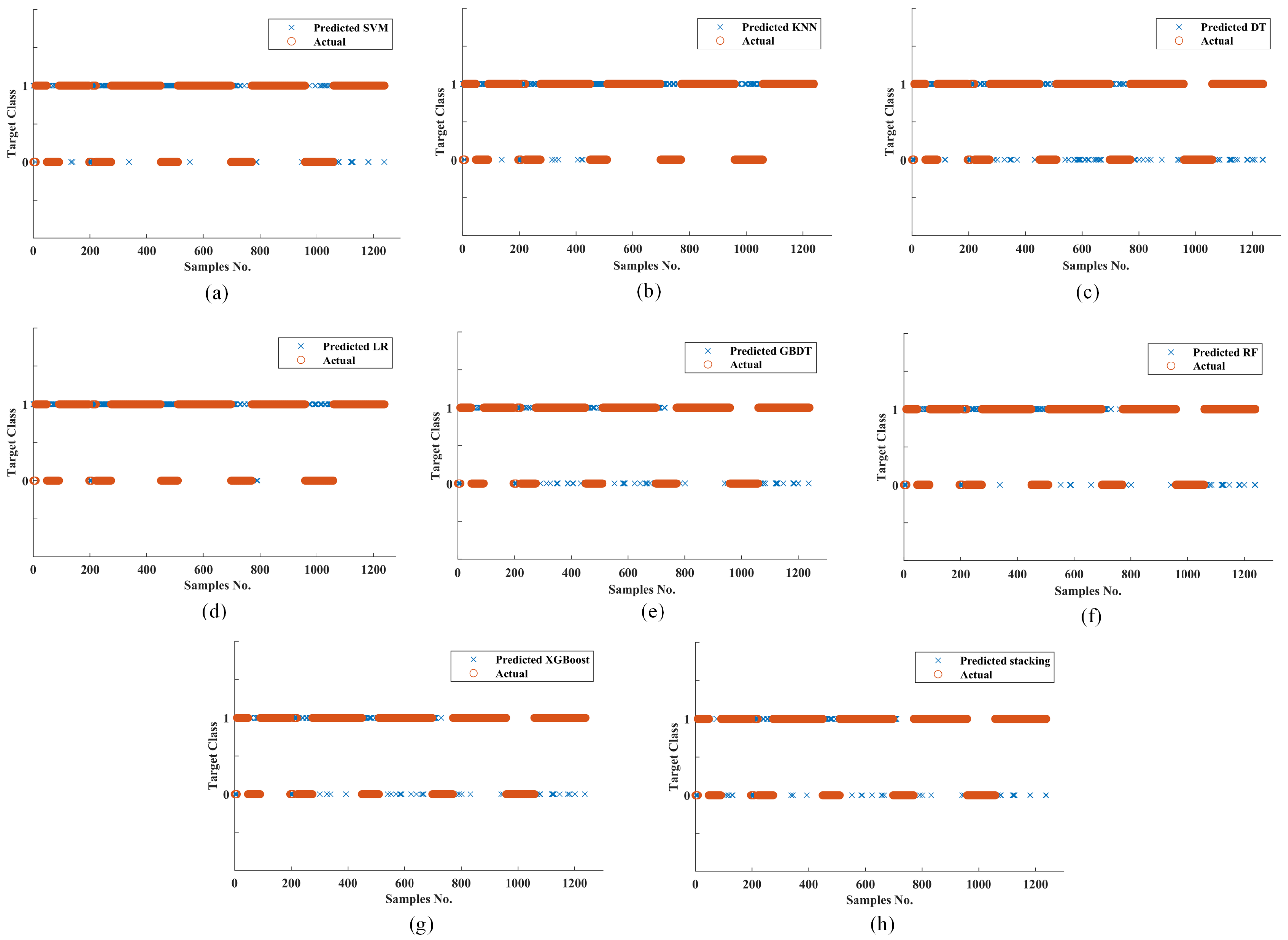
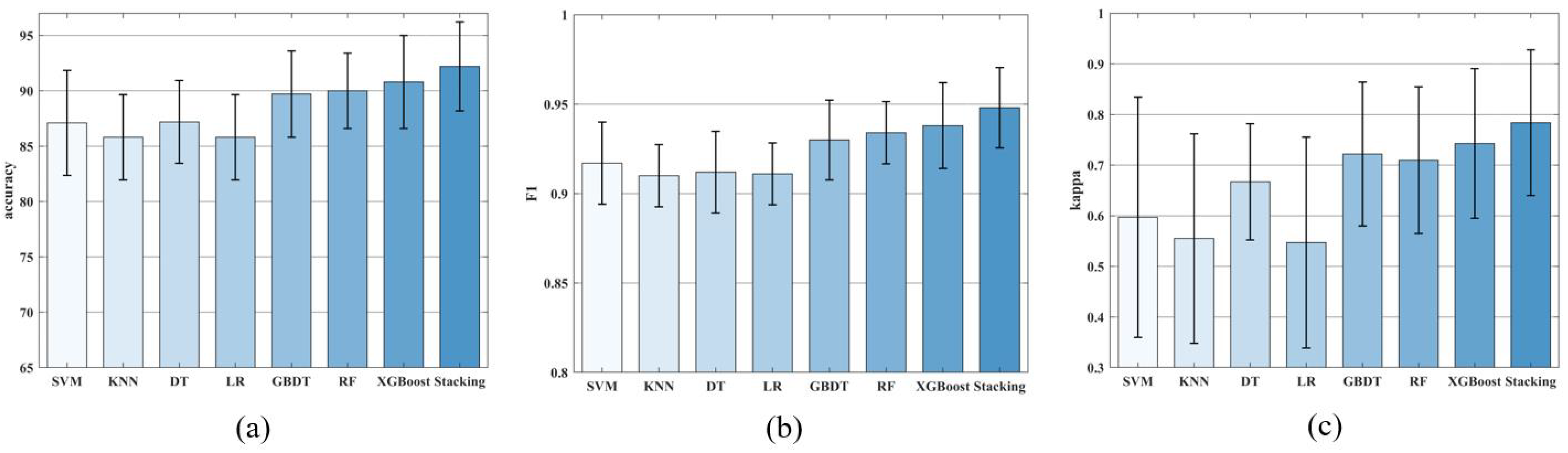
• Compared with other classifiers, the stacking ensemble classifier has the best performance. For $acc$, the stacking ensemble classifier reaches 0.922 ± 0.0402, which is higher than all other eight individual classifiers. For $AUC$, the stacking ensemble classifier reaches 0.958 ± 0.0735, which is higher than all other eight individual classifiers. For $F1$, the stacking ensemble classifier reaches 0.948 ± 0.0225, which is higher than all other eight individual classifiers. For $PRE$, the stacking ensemble classification algorithm reaches 0.941 ± 0.0559, which is higher than all other eight individual classifiers. For $REC$, the stacking ensemble classifier reaches 0.957 ± 0.0257, which is lower than the LR classifier (0.997 ± 0.0072) and RF classifier (0.967 ± 0.0479). It is worth noting that although the LR classifier has a higher REC, the PRE is not high. This phenomenon is due to the imbalanced dataset.
• Tree-based classifiers, such as XGBoost, GBDT, and RF classifiers, have relatively good performance. These classifiers are also ensemble models based on decision trees. This indicates that ensemble classifiers have advantages in classification problems. We use these ensemble models as the base classifiers for the stacking ensemble classifier in this study. For these tree-based classifiers, XGBoost shows the best performance. The $acc$, $AUC$, $F1$, $PRE$, and $REC$ of XGBoost reach 0.908 ± 0.0420 (the best of three ensemble classifiers), 0.950 ± 0.0550 (second only to the RF classifier at 0.956 ± 0.0483), 0.938 ± 0.0240 (the best of the three ensemble models), 0.922 ± 0.0522 (the best of the three ensemble models, equal to the mean of the GBDT classifier, with a standard deviation less than the GBDT classifier), and 0.957 ± 0.0383 (second only to the RF classifier at 0.967 ± 0.0479), respectively.
• The performance of SVM, KNN, LR, and DT classifiers are relatively poorer than that of the stacking ensemble classifier and tree-based classifiers XGBoost, RF, and GBDT. For $acc$, DT has the highest accuracy at 0.872 ± 0.0374, followed by SVM at 0.871 ± 0.0474, and KNN and LR have the worst accuracy at 0.858 ± 0.0384 and 0.858 ± 0.0385, respectively. For $AUC$, SVM has the highest value of 0.945 ± 0.0417; LR takes second place, with a value of 0.932 ± 0.0774; the next is DT, which is 0.890 ± 0.0958; and KNN is the worst, with a value of 0.897 ± 0.0916. For $F1$, all four individual classifiers are greater than 0.9 and relatively close. The $F1$ scores of SVM, KNN, LRm and DT are 0.917 ± 0.0230, 0.910 ± 0.0174, 0.912 ± 0.0228, and 0.911 ± 0.0173, respectively. For $PRE$, only DT is greater than 0.9, at 0.922 ± 0.0509. Furthermore, the PRE values of the other three classifiers are all below 0.9, and the PRE values of SVM, KNN, and LR are 0.868 ± 0.0512, 0.842 ± 0.0314, and 0.839 ± 0.0324, respectively. For $REC$, all four individual classifiers are greater than 0.9. The $REC$ values for SVM, KNN, DT, and LR are 0.975 ± 0.0273, 0.991 ± 0.0149, 0.901 ± 0.0605, and 0.997 ± 0.0072, respectively. This phenomenon is also due to the imbalanced dataset and will be discussed in Section 4.3.2.
• For the $kappa$ coefficient, the stacking ensemble classifier is the highest, at 0.784 ± 0.1437. The three tree class ensemble classifiers XGBoost, RF, and GBDT take second place, with 0.743 ± 0.1479, 0.722 ± 0.1420, and 0.710 ± 0.1450, respectively. The four individual classifiers, SVM, KNN, LR, and DT have relatively low mean values below 0.7, which are 0.597 ± 0.2372, 0.555 ± 0.2070, 0.667 ± 0.1148, and 0.547 ± 0.2085, respectively. This phenomenon reflects the advantage of ensemble classifiers in the processing imbalanced dataset. In conclusion, it can be seen that the stacking ensemble classifier has the best performance. The $acc$, $AUC$, $F1$, $PRE$, and $kappa$ values of the stacking ensemble classifier are the highest among all classifiers. At the same time, the $PRE$ and $REC$ values of the stacking ensemble classifier are relatively balanced, which indicates that the stacking ensemble classifier has strong adaptability to imbalanced datasets. For XGBoost, RF, and GBDT, the results are second only to the stacking ensemble classifier, and their $PRE$ and $REC$ values are both greater than 0.9, indicating that the ensemble classifiers have strong adaptability to imbalanced datasets. For SVM, KNN, LR, and DT, their performances are relatively poor. With the exception of DT, there is a significant gap between the PRE and REC values of the other three individual classifiers. Although cost-sensitive methods were used for the three individual classifiers, the results were still poor.

4.3.2. Prediction Results Based on Relatively Balanced Training Dataset

In this section, all classifiers are trained on the relatively balanced training data based on SMOTE.

Table 5. Optimization results of hyperparameters based on relatively balanced training dataset.

Classifiers	Hyperparameters
SVM	Kernel = ‘$rbf$’, $C=0.9$, $g=0.5$
KNN	$k=6$, weights = distance
DT	Min sample split = 5, min sample leaf = 4, criterion = ‘$gini$’
LR	$C=0.9$, penalty = ‘$l2$’, solver = ‘$sag$’
GBDT	Learning rate = 0.1, n estimators = 110, max depth = 4,
	max features = 5, min sample split = 4, min sample leaf = 4
RF	n estimators = 110, max depth = 6, max features = 5,
	min sample split = 6, min sample leaf = 6
XGBoost	Learning rate = 0.1, n estimators = 110, max depth = 5,
	max features = 5, min sample split = 5, min sample leaf = 5

showcases the hyperparameter optimization outcomes for each classifier.

Table 6. Prediction results based on relatively balanced training dataset.

Classifier	$\mathit{PRE}$	$\mathit{REC}$
SVM	0.913 ± 0.0809	0.943 ± 0.0530
KNN	0.930 ± 0.0865	0.921 ± 0.0583
DT	0.947 ± 0.0484	0.901 ± 0.0285
LR	0.934 ± 0.0827	0.909 ± 0.0527
GBDT	0.938 ± 0.0557	0.937 ± 0.0364
RF	0.931 ± 0.0531	0.943 ± 0.0317
XGBoost	0.945 ± 0.0612	0.943 ± 0.0250
Stacking	0.955 ± 0.0399	0.955 ± 0.0326

shows the PRE and REC values of each classifier on the relatively balanced dataset. Comparing Table 3 and Table 5, it can be seen that all classifiers have closer PRE and REC values on the relatively balanced dataset. Taking the SVM classifier as an example, on the imbalanced dataset, the PRE 5-fold CV mean value and REC 5-fold CV mean value are 0.868 and 0.975, respectively, while on the relatively balanced dataset, both values are 0.913 and 0.943, respectively. It is worth noting that the PRE 5-fold CV mean value and REC 5-fold CV mean value of the ensemble classifiers, including the proposed stacking ensemble classifier, XGBoost, GBDT, and RF, show relatively little change. This phenomenon also indicates that compared to classical classifiers, ensemble classifiers have more advantages on imbalanced datasets compared with individual classifiers.

In order to further analyze the impact of imbalanced datasets on classifiers, the metrics introduced in Section 2 were calculated, including accuracy, AUC, F1, and kappa.

Table 7. Predicted $acc$ changes based on the imbalanced training dataset and the relatively balanced training dataset.

Classifier	Imbalanced	Relatively Balanced	Mean Variation (%)
SVM	0.871 ± 0.0474	0.886 ± 0.0478	1.5
KNN	0.858 ± 0.0384	0.884 ± 0.0476	2.6
DT	0.872 ± 0.0374	0.890 ± 0.0375	1.8
LR	0.858 ± 0.0385	0.881 ± 0.0404	2.3
GBDT	0.897 ± 0.0390	0.906 ± 0.0416	0.9
RF	0.900 ± 0.0340	0.908 ± 0.0393	0.8
XGBoost	0.908 ± 0.0420	0.914 ± 0.0445	0.6
Stacking	0.922 ± 0.0402	0.933 ± 0.0472	1.1

,

Table 8. Predicted $AUC$ changes based on the imbalanced training dataset and the relatively balanced training dataset.

Classifier	Imbalanced	Relatively Balanced	Mean Variation
SVM	0.945 ± 0.0417	0.957 ± 0.0463	0.012
KNN	0.897 ± 0.0916	0.904 ± 0.1039	0.007
DT	0.890 ± 0.0958	0.893 ± 0.0854	0.003
LR	0.932 ± 0.0774	0.938 ± 0.0728	0.006
GBDT	0.934 ± 0.0778	0.945 ± 0.0669	0.011
RF	0.956 ± 0.0483	0.951 ± 0.0511	−0.005
XGBoost	0.950 ± 0.0550	0.944 ± 0.0747	−0.006
Stacking	0.958 ± 0.0735	0.962 ± 0.0606	0.004

,

Table 9. Predicted $F1$ changes based on the imbalanced training dataset and the relatively balanced training dataset.

Classifier	Imbalanced	Relatively Balanced	Mean Variation
SVM	0.917 ± 0.0230	0.924 ± 0.0225	0.007
KNN	0.910 ± 0.0174	0.921 ± 0.0218	0.011
DT	0.912 ± 0.0228	0.923 ± 0.0209	0.011
LR	0.911 ± 0.0173	0.918 ± 0.0175	0.007
GBDT	0.930 ± 0.0223	0.936 ± 0.0241	0.006
RF	0.934 ± 0.0174	0.938 ± 0.0221	0.004
XGBoost	0.938 ± 0.0240	0.942 ± 0.0250	0.004
Stacking	0.948 ± 0.0225	0.951 ± 0.0278	0.003

and

Table 10. Predicted $kappa$ changes based on the imbalanced training dataset and the relatively balanced training dataset.

Classifier	Imbalanced	Relatively Balanced	Mean Variation
SVM	0.597 ± 0.2372	0.668 ± 0.2258	0.071
KNN	0.555 ± 0.2070	0.661 ± 0.2371	0.106
DT	0.667 ± 0.1148	0.720 ± 0.1227	0.053
LR	0.547 ± 0.2085	0.668 ± 0.1910	0.121
GBDT	0.722 ± 0.1420	0.748 ± 0.1468	0.026
RF	0.710 ± 0.1450	0.747 ± 0.1435	0.037
XGBoost	0.743 ± 0.1479	0.766 ± 0.1580	0.023
Stacking	0.784 ± 0.1437	0.821 ± 0.1341	0.037

show the $acc$, $AUC$, $F1$, $kappa$, and mean variation between the imbalanced and relatively balanced datasets. The following can be observed from the tables:

• For $acc$, all classifiers improved differently on the relatively balanced dataset. The mean accuracy of SVM, KNN, DT, LR, GBDT, RF, XGBoost, and the stacking ensemble classifier increased by $1.5\%$, 2.6%, 1.8%, 2.3%, 0.9%, 0.8%, 0.6%, and 1.1%, respectively. It is worth noting that the accuracy increase in the ensemble classifiers represented by the stacking ensemble classifier is lower than that of the individual classifiers, which also indicates that the ensemble classifiers have advantages in processing imbalanced datasets. In addition, the accuracy increase in the stacking ensemble classifier is greater than that of the GBDT, RF, and XGBoost ensemble classifiers. This phenomenon can be attributed to the accuracy increase in the base classifiers. The use of SMOTE has led to a relatively balanced training dataset, resulting in improved performance for individual classifiers. The moderately balanced dataset reduces the risk of classifier overfitting and ultimately enhances the evaluation metrics for the classifier. Due to the improved performance of base classifiers, the final stacking ensemble model also shows improvement.
• For $AUC$, it can be found that, with the exception of the RF (a decrease of 0.005) and XGBoost (a decrease of 0.006) classifiers, the AUC values of all other classifiers increased. Among them, the SVM classifier has the highest improvement of 0.012, and DT showed the lowest improvement of 0.003.
• It can be found that all classifiers have varying degrees of increases in $F1$. Among them, KNN and DT have the largest increase, at 0.011, and the stacking ensemble classifier shows the smallest increase of 0.003. Obviously, the improvement values of the ensemble classifiers are smaller than that of the individual classifier, which also reflects the advantage of the ensemble classifiers in processing imbalanced datasets.
• The $kappa$ coefficients of all classifiers increased, with the LR classifier showing an improvement value of 0.121 and XGBoost showing an improvement value of 0.023, which is the smallest. This phenomenon not only reflects the enhanced separability of the dataset after SMOTE oversampling but also the effectiveness of oversampling from another perspective.

4.4. Model Deployment on Embedded Systems

We have deployed the optimal stacking ensemble model trained on a balanced dataset on an NVIDIA AGX Orin, a powerful embedded system chip with a maximum computational power of 275 TOPS. Using a socket connection, we established duplex communication between the UAHW and the NVIDIA AGX Orin. The specific computational process involves UAHW computing echo features and transmitting them to the NVIDIA AGX Orin through the socket connection. The NVIDIA AGX Orin computes the predicted results and transmits them back to UAHW. Through testing, the stacking ensemble model has demonstrated accurate predictions with a time of 15 ms, meeting the real-time requirements of UAHWs.

5. Discussion

In this study, we propose an underwater intelligent target recognition method for underwater acoustic homing weapons based on stacking ensemble technology. The analysis results indicate that this method possesses stronger recognition and generalization capabilities compared to individual classification models. Additionally, as our approach utilizes highlight detection for feature extraction, it can be easily extended to the problem of point source acoustic decoy recognition. As shown in

Table 11. A comparison with existing methods.

Method	Point Source Decoy Recognition Capability	Scale Decoy Recognition Capability	Real-Time Capability
Ours	Scalable	Possesses	Possesses
The literature [2]	Possesses	Does not possess	Possesses
The literature [3]	Possesses	Does not possess	Possesses
The literature [34]	Possesses	Does not possess	Possesses

, after comparison with some existing scale target recognition methods for underwater acoustic homing weapons, our proposed method demonstrates applicability to scale acoustic decoy recognition. Furthermore, this method can also be extended to underwater unmanned vehicle (UUV) target recognition.

However, our approach also has certain limitations: when the underwater acoustic homing weapon cannot effectively detect highlights, the model cannot perform effective recognition. Since underwater acoustic homing weapons operate on a multi-cycle working regime, subsequent improvements could leverage this regime. By utilizing detection results from preceding and succeeding cycles to compensate for the lack of detection in a specific cycle, the model could ultimately provide effective recognition results.

6. Conclusions

In this study, we proposed an underwater active acoustic homing classification model based on stacking ensemble technology. The following work was conducted:

• Multiple features based on highlights were extracted from real sea trial data.
• SMOTE oversampling technology was utilized to expand minority scale acoustic decoy data in the feature domain to solve the problem of data imbalance.
• A stacking ensemble classification model was established to improve classification ability and robustness compared to single classification models.
• A semi-physical simulation experiment was conducted on an embedded system, a digital computer was used to calculate features, input them into the embedded system, and provide inference results, proving that the model has real-time performance.

The average recognition $acc$ of the proposed method on sea trial data is 93.3%, with an average $AUC$ of 0.962, average $F1$ of 0.951, average $PRE$ of 0.955, average $REC$ of 0.955, and average $kappa$ of 0.821. The single-cycle inference time is 15 ms. In summary, the method proposed in this study has better performance and robustness compared to traditional single classification models. At the same time, it has good real-time performance and can provide an effective recognition model for UAHWs. In the future, our research will expand in two directions. On the one hand, we will delve into recognition models based on transfer learning. On the other hand, by capitalizing on the multi-cycle operational regime of underwater acoustic homing weapons, our goal is to develop intelligent recognition methods that encompass multiple cycles, allowing for a comprehensive exploration of the implicit information embedded in these operational cycles. This model will be deployed on UAHWs for the purpose of target recognition.

References

1. He, X.Y.; He, G.; Jin, C.; Chen, S.Z. Current Situation and Prospect on Torpedo’s True/False Target Identification Technologies. Torpedo Technol. 2016, 24, 23–27. [Google Scholar]
2. Wang, M.Z.; Hao, C.Y.; Huang, X.W. Underwater Target Dimension Recognition Based on Bearings Analysis of Signal Correlation Feature. J. Northwestern Polytech. Univ. 2003, 21, 317–320. [Google Scholar]
3. Liu, Z.H.; Fu, Z.P.; Wang, M.Z. Underwater Target Identification Based on the Methods of Bearing and Cross-spectrum. Acta Armamentarii 2006, 27, 932–935. [Google Scholar]
4. Fan, S.-H.; Wang, Y.M.; Yue, L.; Kang, W.Y. Underwater Target Simulation System Based on Towed Long Line Array. J. Syst. Simul. 2012, 24, 1083–1087. [Google Scholar]
5. Zhao, Z.; Cai, Z. Simulation and analysis of acoustic linear array decoy for counterworking the torpedo with target scale recognition capability. Tech. Acoust. 2011, 30, 493–495. [Google Scholar]
6. Xu, J.; Huang, Z.; Li, C. Advances in Underwater Target Passive Recognition Using Deep Learning. J. Signal Process. 2019, 35, 1460–1475. [Google Scholar]
7. Luo, X.; Chen, L.; Zhou, H.; Cao, H. A Survey of Underwater Acoustic Target Recognition Methods Based on Machine Learning. J. Mar. Sci. Eng. 2023, 11, 384. [Google Scholar] [CrossRef]
8. Meng, Q.; Yang, S.; Piao, S. The classification of underwater acoustic target signals based on wave structure and support vector machine. J. Acoust. Soc. Am. 2014, 136, 2265. [Google Scholar] [CrossRef]
9. De Moura, N.N.; de Seixas, J.M. Novelty detection in passive SONAR systems using support vector machines. In Proceedings of the 2015 Latin America Congress on Computational Intelligence (LA-CCI), Curitiba, Brazil, 13–16 October 2015; pp. 1–6. [Google Scholar] [CrossRef]
10. Mallat, S.; Zhang, Z. Matching pursuits with time-frequency dictionaries. IEEE Trans. Signal Process. 1993, 41, 3397–3415. [Google Scholar] [CrossRef]
11. Lee, S.; Seo, I.; Seok, J.; Kim, Y.; Han, D.S. Active Sonar Target Classification with Power-Normalized Cepstral Coefficients and Convolutional Neural Network. Appl. Sci. 2020, 10, 8450. [Google Scholar] [CrossRef]
12. Sabara, R.; Jesus, S. Underwater acoustic target recognition using graph convolutional neural networks. J. Acoust. Soc. Am. 2018, 144, 1744. [Google Scholar] [CrossRef]
13. Nguyen, H.T.; Lee, E.H.; Lee, S. Study on the Classification Performance of Underwater Sonar Image Classification Based on Convolutional Neural Networks for Detecting a Submerged Human Body. Sensors 2019, 20, 94. [Google Scholar] [CrossRef] [PubMed]
14. Williams, D.P. Underwater target classification in synthetic aperture sonar imagery using deep convolutional neural networks. In Proceedings of the 2016 23rd International Conference on Pattern Recognition (ICPR), Cancun, Mexico, 4–8 December 2016; pp. 2497–2502. [Google Scholar] [CrossRef]
15. Wang, Y.; Zhang, H.; Xu, L.; Cao, C.; Gulliver, T.A. Adoption of hybrid time series neural network in the underwater acoustic signal modulation identification. J. Frankl. Inst. 2020, 357, 13906–13922. [Google Scholar] [CrossRef]
16. Kamal, S.; Chandran, C.S.; Supriya, M.H. Passive sonar automated target classifier for shallow waters using end-to-end learnable deep convolutional LSTMs. Eng. Sci. Technol. Int. J. 2021, 24, 860–871. [Google Scholar] [CrossRef]
17. Feng, S.; Zhu, X. A Transformer-Based Deep Learning Network for Underwater Acoustic Target Recognition. IEEE Geosci. Remote. Sens. Lett. 2022, 19, 1505805. [Google Scholar] [CrossRef]
18. Gu, J.; Liu, S.; Zhou, Z.; Chalov, S.R.; Zhuang, Q. A Stacking Ensemble Learning Model for Monthly Rainfall Prediction in the Taihu Basin, China. Water 2022, 14, 492. [Google Scholar] [CrossRef]
19. Zhan, Y.; Zhang, H.; Li, J.; Li, G. Prediction Method for Ocean Wave Height Based on Stacking Ensemble Learning Model. J. Mar. Sci. Eng. 2022, 10, 1150. [Google Scholar] [CrossRef]
20. Hou, S.; Liu, Y.; Yang, Q. Real-time prediction of rock mass classification based on TBM operation big data and stacking technique of ensemble learning. J. Rock Mech. Geotech. Eng. 2022, 14, 123–143. [Google Scholar] [CrossRef]
21. Ding, W.; Li, X.; Yang, H.; An, J.; Zhang, Z. A Novel Method for Damage Prediction of Stuffed Protective Structure under Hypervelocity Impact by Stacking Multiple Models. IEEE Access 2020, 8, 130136–130158. [Google Scholar] [CrossRef]
22. Wolpert, D.H. Stacked generalization. Neural Netw. 1992, 5, 241–259. [Google Scholar] [CrossRef]
23. Raghavendra, N.S.; Deka, P.C. Support vector machine application in the field of hydrology: A review. Appl. Soft Comput. 2014, 19, 371–386. [Google Scholar] [CrossRef]
24. Cover, T.M.; Hart, P.E. Nearest neighbor pattern classification. IEEE Trans. Inf. Theory 1953, 13, 21–27. [Google Scholar] [CrossRef]
25. Nowozin, S.; Rother, C.; Bagon, S.; Sharp, T.; Yao, B.; Kohli, P. Decision Tree Fields. In Proceedings of the 2011 International Conference on Computer Vision, Barcelona, Spain, 6–13 November 2011. [Google Scholar]
26. Barros, A.J.; Hirakata, V.N. Alternatives for logistic regression in cross-sectional studies: An empirical comparison of models that directly estimate the prevalence ratio. BMC Med. Res. Methodol. 2003, 3, 21. [Google Scholar] [CrossRef] [PubMed]
27. Tian, R.; Chen, F.; Dong, S. Compound Fault Diagnosis of Stator Interturn Short Circuit and Air Gap Eccentricity Based on Random Forest and XGBoost. Math. Probl. Eng. 2021, 2021, 2149048. [Google Scholar] [CrossRef]
28. Friedman, J.H. Greedy Function Approximation: A Gradient Boosting Machine. Ann. Stat. 2000, 29, 1189–1232. [Google Scholar] [CrossRef]
29. He, J.; Hao, Y.; Wang, X. An Interpretable Aid Decision-Making Model for Flag State Control Ship Detention Based on SMOTE and XGBoost. J. Mar. Sci. Eng. 2021, 9, 156. [Google Scholar] [CrossRef]
30. Chawla, N.V.; Bowyer, K.W.; Hall, L.O.; Kegelmeyer, W.P. SMOTE: Synthetic minority over-sampling technique. AI Access Found. 2002, 16, 321–357. [Google Scholar] [CrossRef]
31. Wang, M.; Huang, X.; Hao, C. Model of an Underwater Target Based on Target Echo Highlight Structure. J. Syst. Simul. 2003, 15, 5. [Google Scholar]
32. Cheng, J.; Liu, H.; Wang, F.; Li, H.; Zhu, C. Silhouette analysis for human action recognition based on supervised temporal t-SNE and incremental learning. IEEE Trans. Image Process. 2015, 24, 3203–3217. [Google Scholar] [CrossRef]
33. Feurer, M.; Hutter, F. Hyperparameter Optimization. In Automated Machine Learning: Methods, Systems, Challenges; Hutter, F., Kotthoff, L., Vanschoren, J., Eds.; Springer International Publishing: Cham, Switzerland, 2019; pp. 3–33. [Google Scholar] [CrossRef]
34. Zhang, J.; Jiang, X.-Z.; Chen, X. Way of Identifying Target Based on Covariance of Bearing Fluctuation. J. Nav. Univ. Eng. 2005, 17, 91–96. [Google Scholar]
Figure 2. UAHW target recognition algorithm flowchart.
Jmse 11 02305 g002
Figure 3. Signal detection process diagram.
Jmse 11 02305 g003
Figure 4. Time-varying gain control diagram.
Jmse 11 02305 g004
Figure 5. Time-domain signal after TVG processing result.
Jmse 11 02305 g005
Figure 6. (a) Frequency-domain signal before TVG processing result. (b) Frequency-domain signal after TVG processing result.
Jmse 11 02305 g006
Figure 7. Signal detection process flowchart.
Jmse 11 02305 g007
Figure 8. Signal correlation detection flowchart.
Jmse 11 02305 g008
Figure 9. Signal frequency-domain correlation detection.
Jmse 11 02305 g009
Figure 10. The t-SNE visualization results for the 5-fold cross-validation of features.
Jmse 11 02305 g010
Figure 12. Stacking ensemble model construction diagram.
Jmse 11 02305 g012
Figure 13. Predictive results of each classifier based on imbalanced training dataset: (a) SVM; (b) KNN; (c) DT; (d) LR; (e) GBDT; (f) RF; (g) XGBoost; (h) stacking.
Jmse 11 02305 g013
Figure 14. Prediction results of each classifier based on imbalanced training dataset: (a a c c ; (b F 1 ; (c k a p p a .
Jmse 11 02305 g014