
Speed Optimization in Bulk Carriers: A Weather-Sensitive Approach for Reducing Fuel Consumption


Abstract
:1. Introduction
2. Problem Description and Model Establishment
2.1. Problem Description
- The main engine is the sole consumer of fuel on the ship.
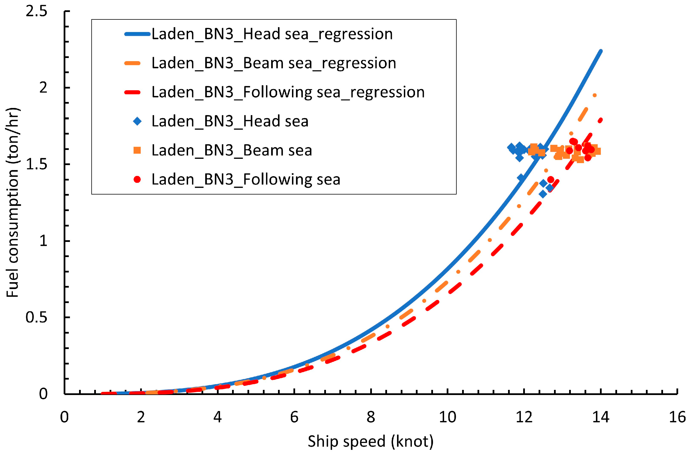
- BN and weather direction are the environmental factors affecting the fuel consumption curves.
- BN and weather direction remain constant for a 1 h duration within a leg of the journey.
- BN and weather direction of a leg are only determined by the arrival time of the leg.
- Ship speed is maintained consistently throughout each leg.
- The loading condition is either laden or ballast.
- The allowable arrival time remains constant across all waypoints.
- The ship only uses a single type of fuel.
2.2. Fuel Consumption Model
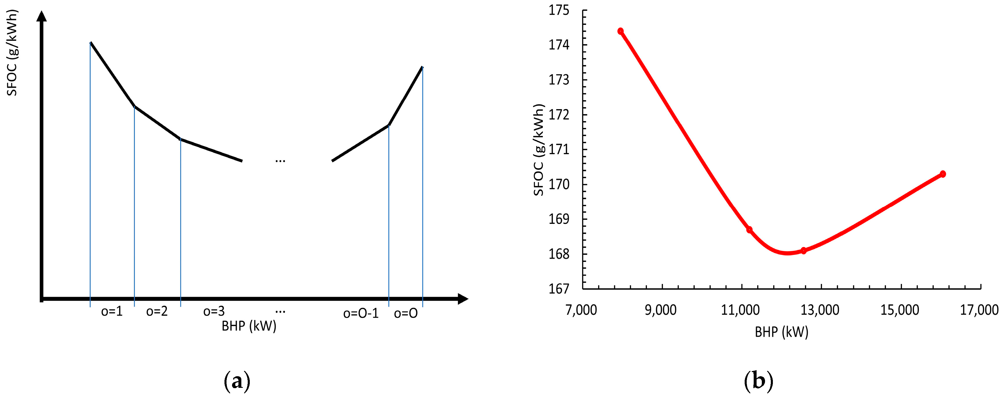
2.2.1. First Approach
2.2.2. Second Approach
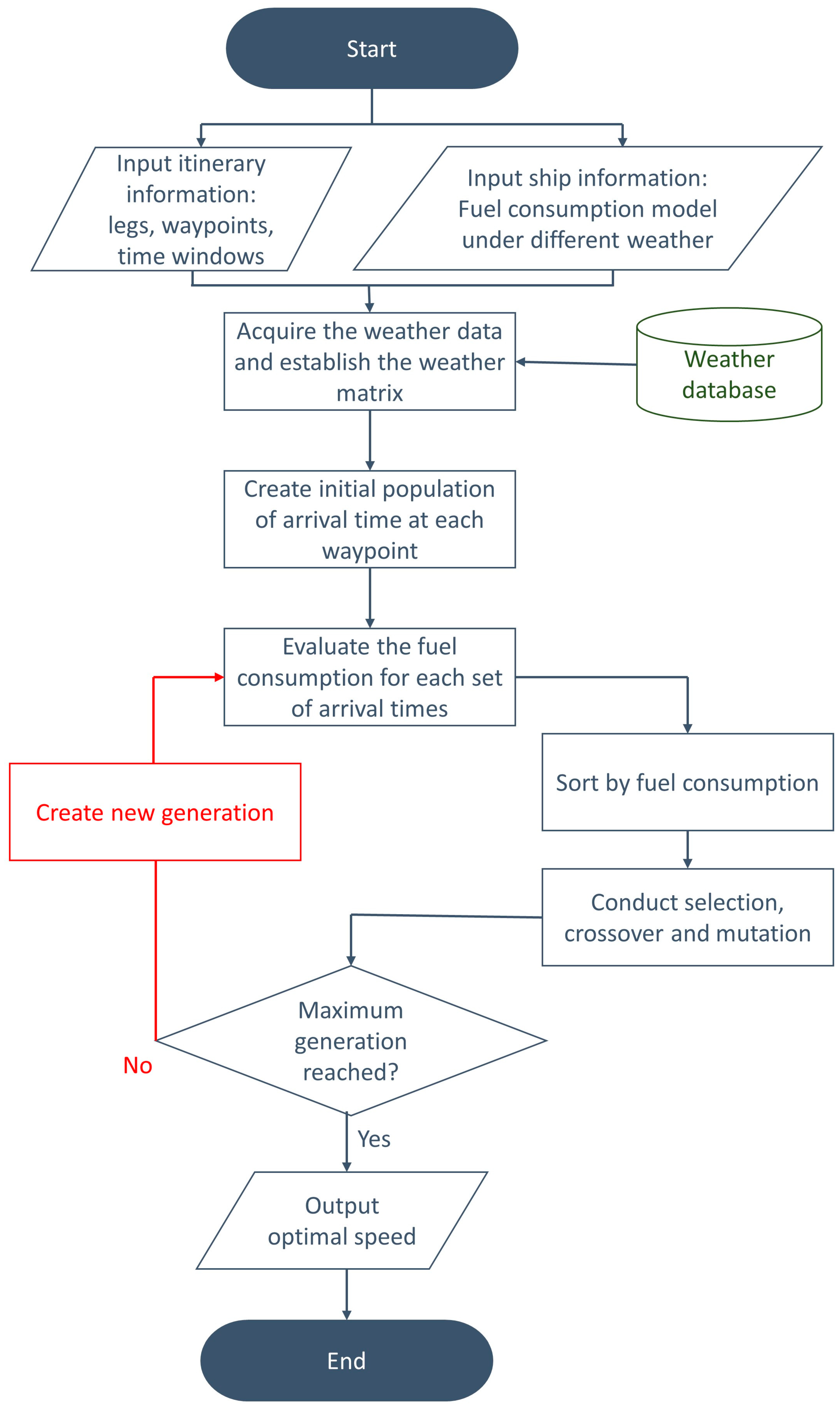
2.3. Optimization Algorithm
2.4. Mathematical Model
3. Results and Discussion
3.1. Case Study
3.1.1. Case Study 1—93,000 DWT Bulk Carrier
3.1.2. Case Study 2—200,000 DWT Bulk Carrier
3.2. Sensitivity Analysis
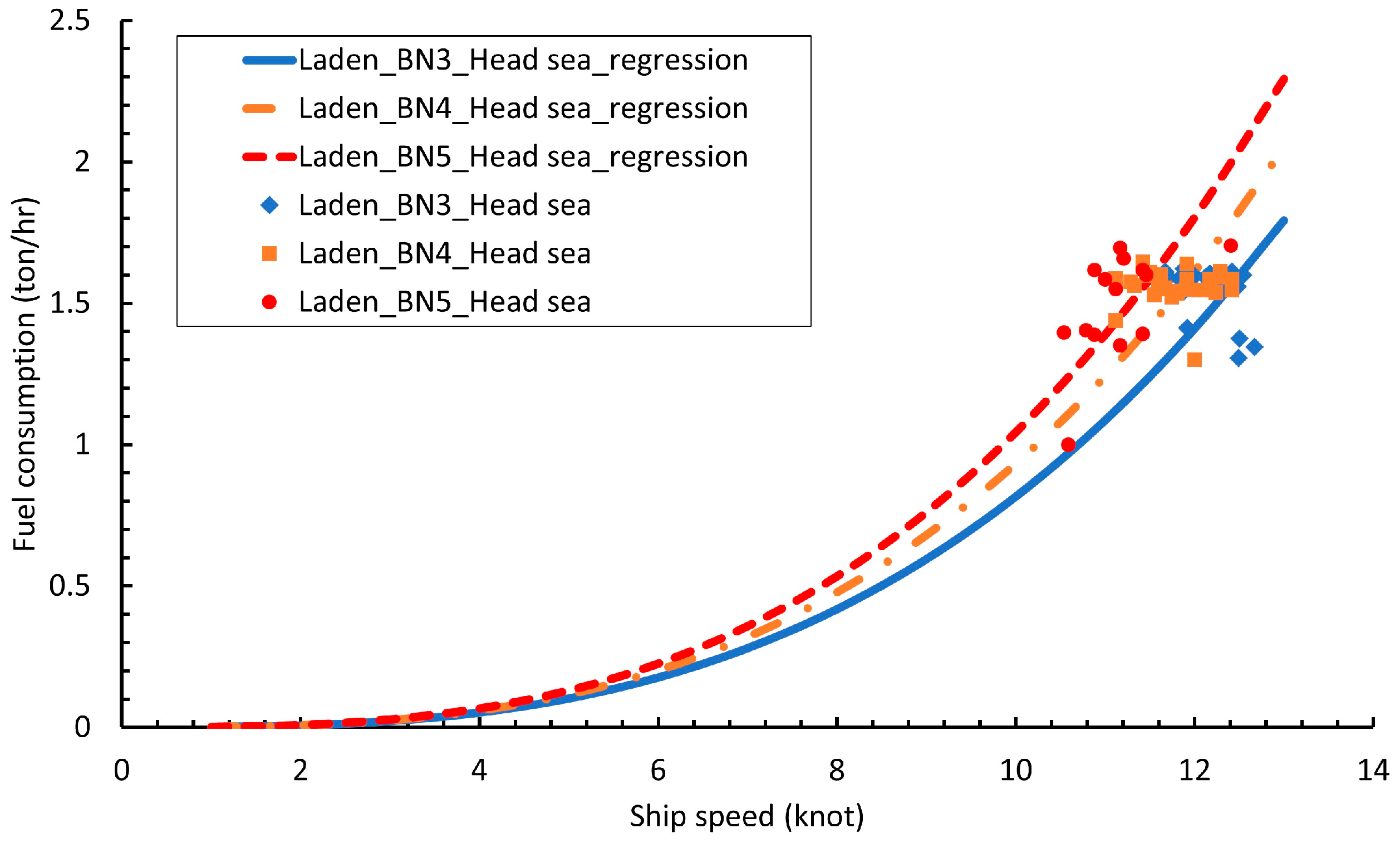
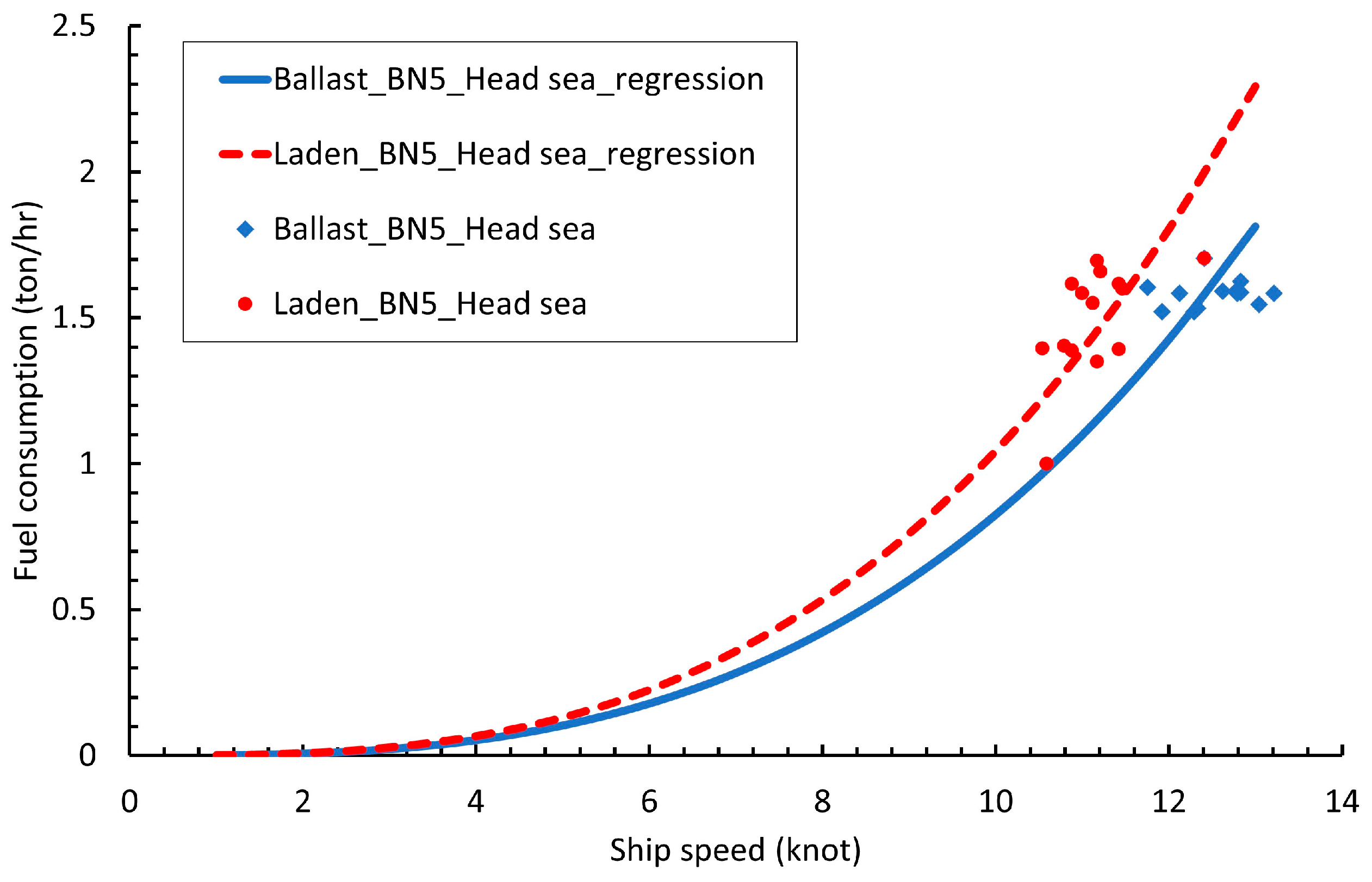
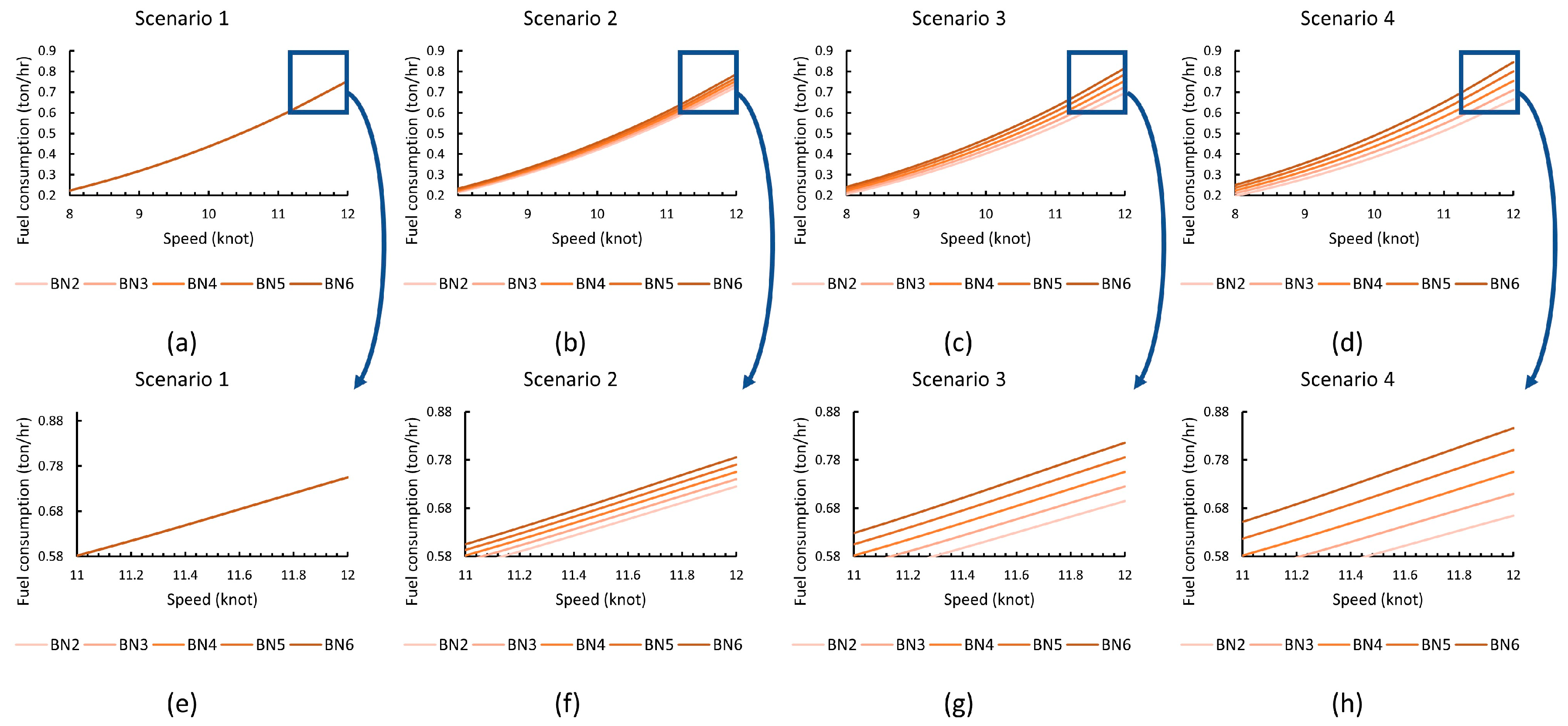
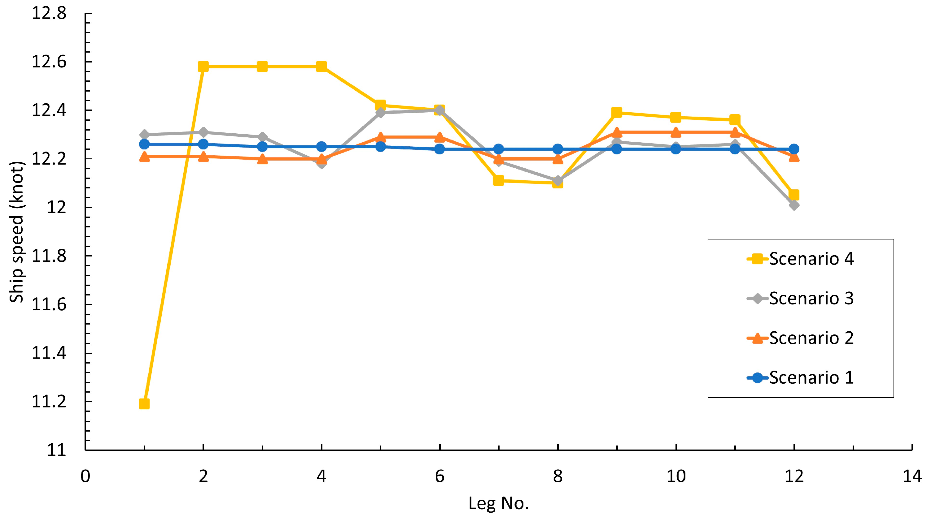
3.2.1. Effects of Different BN-Affected Speed–Fuel Consumption Curves
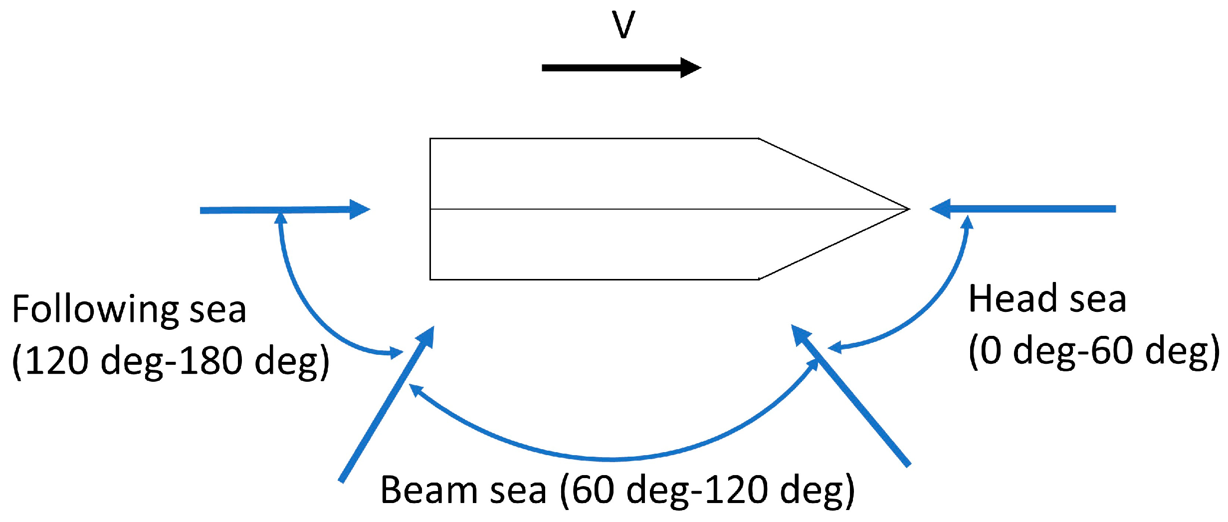
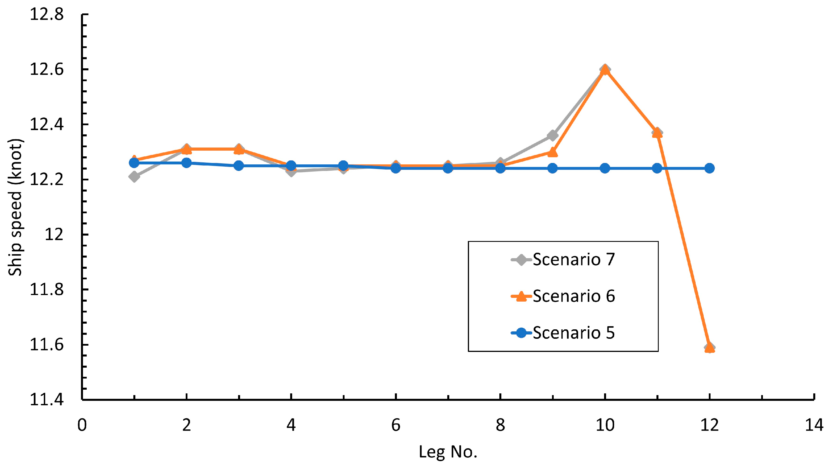
3.2.2. Effects of Different Weather Direction-Affected Speed–Fuel Consumption Curves
3.2.3. Effects of Different Total Sailing Time
4. Conclusions and Prospects
Author Contributions
Funding
Institutional Review Board Statement
Informed Consent Statement
Data Availability Statement
Conflicts of Interest
Nomenclature and List of Abbreviations
| Symbol | Unit | Explanation |
| Abbreviations | ||
| BHP | Brake horsepower | |
| BN | Beaufort number | |
| DWT | Deadweight tonnage | |
| GA | Genetic algorithm | |
| GHG | Greenhouse gas | |
| IMO | International Maritime Organization | |
| SFOC | Specific fuel oil consumption | |
| Indices and sets | ||
| N | Set of all waypoints (legs) on the ship route, | |
| S | Set of all BNs on the ship route, | |
| P | Set of all weather directions on the ship route, | |
| O | Set of all linear segments of the simulation of BHP-SFOC relationship, | |
| Parameters | ||
| ton | Calculated fuel consumption for the whole itinerary. Objective to be minimized | |
| h | Accumulated acceptable earliest arrival time at each waypoint | |
| M | h | Fixed allowable arrival time interval at each waypoint |
| Main engine fuel consumption–speed coefficient of BN s and weather direction p for leg n in the sailing period | ||
| Main engine fuel consumption–speed power coefficient of BN s and weather direction p for leg n in the sailing period | ||
| nm | Sailing distance for leg n | |
| knot | Ship speed over ground for leg n in the sailing period | |
| h | Sailing period for leg n | |
| Binary, equals 1 if and only if the equals s in leg n; 0 otherwise | ||
| Binary, equals 1 if and only if the equals p in leg n; 0 otherwise | ||
| BN encountered when the arrival time of waypoint-n equals | ||
| Weather direction encountered when the arrival time of waypoint-n equals | ||
| Main engine BHP-SFOC first-order coefficient of segment o | ||
| Main engine BHP-SFOC coefficient of segment o | ||
| Main engine Speed-BHP coefficient of BN s in the sailing period | ||
| Main engine Speed-BHP power coefficient of BN s in the sailing period | ||
| Decision variables | ||
| Accumulated arrival time of waypoint-n |
References
- IMO. Resolution MEPC.377(80), 2023 IMO Strategy on Reduction of GHG Emissions from Ships; International Maritime Organization: London, UK, 2023. [Google Scholar]
- Fagerholt, K.; Laporte, G.; Norstad, I. Reducing fuel emissions by optimizing speed on shipping routes. J. Oper. Res. Soc. 2010, 61, 523–529. [Google Scholar] [CrossRef]
- Gao, C.-F.; Hu, Z.-H. Speed Optimization for Container Ship Fleet Deployment Considering Fuel Consumption. Sustainability 2021, 13, 5242. [Google Scholar] [CrossRef]
- Lu, J.; Wu, X.; Wu, Y. The Construction and Application of Dual-Objective Optimal Speed Model of Liners in a Changing Climate: Taking Yang Ming Route as an Example. J. Mar. Sci. Eng. 2023, 11, 157. [Google Scholar] [CrossRef]
- Shih, Y.-C.; Tzeng, Y.-A.; Cheng, C.-W.; Huang, C.-H. Speed and Fuel Ratio Optimization for a Dual-Fuel Ship to Minimize Its Carbon Emissions and Cost. J. Mar. Sci. Eng. 2023, 11, 758. [Google Scholar] [CrossRef]
- Wang, Z.; Fan, A.; Tu, X.; Vladimir, N. An energy efficiency practice for coastal bulk carrier: Speed decision and benefit analysis. Reg. Stud. Mar. Sci. 2021, 47, 101988. [Google Scholar] [CrossRef]
- Li, X.; Sun, B.; Guo, C.; Du, W.; Li, Y. Speed optimization of a container ship on a given route considering voluntary speed loss and emissions. Appl. Ocean Res. 2020, 94, 101995. [Google Scholar] [CrossRef]
- Yang, L.; Chen, G.; Zhao, J.; Rytter, N.G.M. Ship Speed Optimization Considering Ocean Currents to Enhance Environmental Sustainability in Maritime Shipping. Sustainability 2020, 12, 3649. [Google Scholar] [CrossRef]
- Zhuge, D.; Wang, S.; Wang, D.Z.W. A joint liner ship path, speed and deployment problem under emission reduction measures. Transp. Res. Part B Methodol. 2021, 144, 155–173. [Google Scholar] [CrossRef]
- Ballou, P.; Henry, C.; John, D. Horner, Advanced Methods of Optimizing Ship Operations to Reduce Emissions Detrimental to Climate Change. In Proceedings of the Oceans 2008, Quebec City, QC, Canada, 15–18 September 2008; pp. 1–12. [Google Scholar] [CrossRef]
- Song, S.; Demirel, Y.K.; Atlar, M.; Dai, S.; Day, S.; Turan, O. Validation of the CFD approach for modelling roughness effect on ship resistance. Ocean Eng. 2020, 200, 107029. [Google Scholar] [CrossRef]
- Chirosca, A.-M.; Medina, A.; Pacuraru, F.; Saettone, S.; Rusu, L.; Pacuraru, S. Experimental and Numerical Investigation of the Added Resistance in Regular Head Waves for the DTC Hull. J. Mar. Sci. Eng. 2023, 11, 852. [Google Scholar] [CrossRef]
- Tadros, M.; Ventura, M.; Guedes Soares, C. Effect of Hull and Propeller Roughness during the Assessment of Ship Fuel Consumption. J. Mar. Sci. Eng. 2023, 11, 784. [Google Scholar] [CrossRef]
- Kwon, Y.J. Speed loss due to added resistance in wind and waves. Nav. Archit. 2008, 3, 14–16. [Google Scholar]
- Kuroda, M.; Tsujimoto, M.; Fujiwara, T.; Ohmatsu, S.; Takagi, K. Investigation on components of added resistance in short waves. J. Jpn. Soc. Nav. Archit. Ocean Eng. 2008, 8, 171–176. [Google Scholar] [CrossRef]
- Lu, R.; Turan, O.; Boulougouris, E.; Banks, C.; Incecik, A. A semi-empirical ship operational performance prediction model for voyage optimization towards energy efficient shipping. Ocean Eng. 2015, 110, 18–28. [Google Scholar] [CrossRef]
- Kim, K.J.; Lee, S.D.; Jun, C.H.; Park, K.M.; Byeon, S.S. A statistical procedure of analyzing container ship operation data for finding fuel consumption patterns. Korean J. Appl. Stat. 2017, 30, 633–645. [Google Scholar] [CrossRef]
- Adland, R.; Cariou, P.; Wolff, F.-C. Optimal ship speed and the cubic law revisited: Empirical evidence from an oil tanker fleet. Transp. Res. Part E Logist. Transp. Rev. 2020, 140, 101972. [Google Scholar] [CrossRef]
- Wang, S.; Ji, B.; Zhao, J.; Liu, W.; Xu, T. Predicting ship fuel consumption based on LASSO regression. Transp. Res. Part D Transp. Environ. 2018, 65, 817–824. [Google Scholar] [CrossRef]
- Karagiannidis, P.; Themelis, N.; Zaraphonitis, G.; Spandonidis, C.; Giordamlis, C. Ship Fuel Consumption Prediction using Artificial Neural Networks. In Proceedings of the Annual Meeting of Marine Technology Conference Proceedings, Athens, Greece, 26 November 2019; pp. 46–51. [Google Scholar]
- Kim, Y.-R.; Jung, M.; Park, J.-B. Development of a Fuel Consumption Prediction Model Based on Machine Learning Using Ship In-Service Data. J. Mar. Sci. Eng. 2021, 9, 137. [Google Scholar] [CrossRef]
- Beşikçi, E.B.; Arslan, O.; Turan, O.; Ölçer, A.I. An artificial neural network based decision support system for energy efficient ship operations. Comput. Oper. Res. 2016, 66, 393–401. [Google Scholar] [CrossRef]
- Blendermann, W. Parameter identification of wind loads on ships. J. Wind. Eng. Ind. Aerodyn. 1994, 51, 339–351. [Google Scholar] [CrossRef]
- Bialystocki, N.; Konovessis, D. On the estimation of ship’s fuel consumption and speed curve: A statistical approach. J. Ocean Eng. Sci. 2016, 1, 157–166. [Google Scholar] [CrossRef]
- Blank, J.; Deb, K. Pymoo: Multi-Objective Optimization in Python. IEEE Access 2020, 8, 89497–89509. [Google Scholar] [CrossRef]
- Tzortzis, G.; Sakalis, G. A dynamic ship speed optimization method with time horizon segmentation. Ocean Eng. 2021, 226, 108840–108853. [Google Scholar] [CrossRef]
- Vettor, R.; Bergamini, G.; Guedes Soares, C. A Comprehensive Approach to Account for Weather Uncertainties in Ship Route Optimization. J. Mar. Sci. Eng. 2021, 9, 1434. [Google Scholar] [CrossRef]
- Vettor, R.; Soares, C.G. Reflecting the uncertainties of ensemble weather forecasts on the predictions of ship fuel consumption. Ocean Eng. 2021, 250, 111009. [Google Scholar] [CrossRef]
- Weile, D.S.; Michielssen, E. Genetic algorithm optimization applied to electromagnetics: A review. IEEE Trans. Antennas Propag. 1997, 45, 343–353. [Google Scholar] [CrossRef]
- Cus, F.; Balic, J. Optimization of cutting process by GA approach. Robot. Comput.-Integr. Manuf. 2003, 19, 113–121. [Google Scholar] [CrossRef]
- Fernandez, M.; Caballero, J.; Fernandez, L.; Sarai, A. Genetic algorithm optimization in drug design QSAR: Bayesian-regularized genetic neural networks (BRGNN) and genetic algorithm-optimized support vectors machines (GA-SVM). Mol. Divers. 2011, 15, 269–289. [Google Scholar] [CrossRef]
- Johnson, J.M.; Rahmat-Samii, Y. Genetic algorithm optimization and its application to antenna design. In Proceedings of the IEEE Antennas and Propagation Society International Symposium and URSI National Radio Science Meeting, Seattle, WA, USA, 20–24 June 1994; pp. 326–329. [Google Scholar]
- Abdelmegid, M.A.; Shawki, K.M.; Abdel-Khalek, H. GA optimization model for solving tower crane location problem in construction sites. Alex. Eng. J. 2015, 54, 519–526. [Google Scholar] [CrossRef]
- Fitzgerald, J.; Wong-Lin, K. Multi-objective optimisation of cortical spiking neural networks with genetic algorithms. In Proceedings of the 2021 32nd Irish Signals and Systems Conference (ISSC), Athlone, Ireland, 10–11 June 2021; pp. 1–6. [Google Scholar]
- Khan, A.; Deb, K. Optimizing Keyboard Configuration Using Single and Multi-Objective Evolutionary Algorithms. In Proceedings of the Companion Conference on Genetic and Evolutionary Computation, Lisbon, Portugal, 24 July 2023; pp. 219–222. [Google Scholar]
- Deb, K.; Sindhya, K.; Okabe, T. Self-adaptive simulated binary crossover for real-parameter optimization. In Proceedings of the 9th Annual Conference on Genetic and Evolutionary Computation, GECCO ’07, New York, NY, USA, 7–11 July 2007; pp. 1187–1194. [Google Scholar] [CrossRef]
- Wiesmann, A. Slow steaming—A viable long-term option. Wartsila Tech. J. 2010, 2, 49–55. [Google Scholar]


| Papers | Year | Optimization Objectives | Optimization Variables | Algorithms | Ship Type | Considering Two-Port Itinerary | Variable Weather Condition for Different Arrival Time |
|---|---|---|---|---|---|---|---|
| Fagerholt et al. [2] | 2010 | Minimizing fuel consumption | Speed | IPOPT from COIN-OR | Not specified | No | No |
| Li et al. [7] | 2020 | Minimizing the fuel consumption and costs | Speed | constrained optimization by linear approximation (COBYLA) | Container ship | Yes | No |
| Yang et al. [8] | 2020 | Minimizing fuel consumption | Speed | GA | Oil tanker | Yes | No |
| Zhuge et al. [9] | 2021 | Minimizing cost | Joint ship path, speed, and deployment | Dynamic programming-based method | Not specified | Yes | No |
| Gao and Hu [3] | 2021 | Minimizing cost | Speed and fleet deployment | Linear outer-approximation algorithm and an improved piecewise linear approximation algorithm | Container ship | No | No |
| Wang et al. [6] | 2021 | Minimizing fuel consumption | Main engine speed | NSGA-II | Bulk carrier | Yes | No |
| Lu et al. [4] | 2023 | Minimizing cost and carbon emissions | Speed | MOPSO | Container ship | No | No |
| Shih et al. [5] | 2023 | Minimizing cost and carbon emissions | Fuel ratio and speed | NSGA-II | Container ship | No | No |
| Present study | Minimizing fuel consumption | Speed | GA | Bulk carrier | Yes | Yes |
| [Beaufort Number, Weather Direction] | ⋯ | ||||
|---|---|---|---|---|---|
| Waypoint-1 | [ | ⋯ | |||
| Waypoint-2 | ⋯ | ||||
| Waypoint-3 | ⋯ | ||||
| Waypoint-N | ⋯ |
| Target Ship A | Target Ship B | |
|---|---|---|
| Length overall (m) | 235 | 300 |
| Breath (m) | 38 | 50 |
| Depth (m) | 20 | 25 |
| Deadweight (ton) | 93,000 | 200,000 |
| Complete year | 2011 | 2013 |
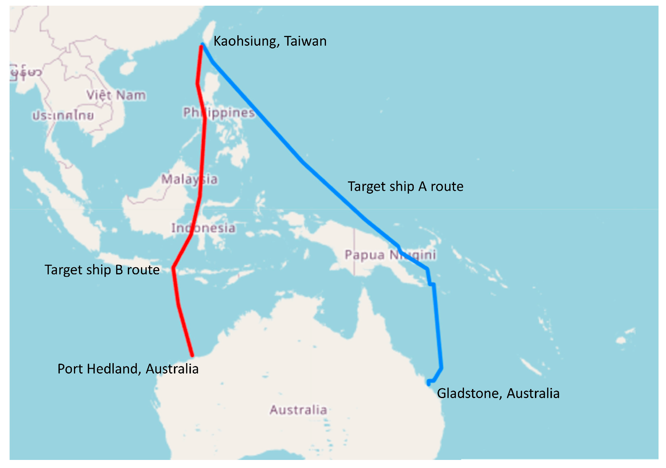
| Operation route | Kaohsiung, Taiwan—Gladstone, Australia | Port Hedland, Australia—Kaoshiung, Taiwan |
| Leg No. | Arrival Port/Waypoint | Acceptable Earliest Arrival Time | Acceptable Latest Arrival Time | Sailing Distance (nm) |
|---|---|---|---|---|
| P1-TWKHH | 26 May 12:00 | 26 May 12:00 | ||
| 1 | Waypoint 1 | 26 May 12:00 | 7 June 10:00 | 302.00 |
| 2 | Waypoint 2 | 26 May 12:00 | 7 June 10:00 | 301.00 |
| 3 | Waypoint 3 | 26 May 12:00 | 7 June 10:00 | 279.00 |
| 4 | Waypoint 4 | 26 May 12:00 | 7 June 10:00 | 263.00 |
| 5 | Waypoint 5 | 26 May 12:00 | 7 June 10:00 | 299.00 |
| 6 | Waypoint 6 | 26 May 12:00 | 7 June 10:00 | 295.00 |
| 7 | Waypoint 7 | 26 May 12:00 | 7 June 10:00 | 267.00 |
| 8 | Waypoint 8 | 26 May 12:00 | 7 June 10:00 | 279.00 |
| 9 | Waypoint 9 | 26 May 12:00 | 7 June 10:00 | 292.00 |
| 10 | Waypoint 10 | 26 May 12:00 | 7 June 10:00 | 315.00 |
| 11 | Waypoint 11 | 26 May 12:00 | 7 June 10:00 | 297.00 |
| 12 | P2-AUGLT | 7 June 10:00 | 7 June 10:00 | 313.00 |
| Original Sailing Mode | Recommended Sailing Mode | |||||||
|---|---|---|---|---|---|---|---|---|
| Leg No. | Original Arrival Time (UTC +8) | Original Speed (Knot) | BN | Weather Direction | Recommended Arrival Time (UTC +8) | Recommended Speed (Knot) | BN | Weather Direction |
| 26 May 12:00 | - | 26 May 12:00 | - | - | ||||
| 1 | 27 May 12:00 | 12.58 | 4 | Beam sea | 27 May 13:02 | 12.07 | 4 | Beam sea |
| 2 | 28 May 12:00 | 12.54 | 4 | Following sea | 28 May 12:57 | 12.58 | 4 | Following sea |
| 3 | 29 May 11:00 | 12.13 | 4 | Following sea | 29 May 11:10 | 12.58 | 4 | Following sea |
| 4 | 30 May 11:00 | 10.96 | 5 | Beam sea | 30 May 08:57 | 12.08 | 4 | Beam sea |
| 5 | 31 May 11:00 | 12.46 | 3 | Beam sea | 31 May 09:35 | 12.15 | 3 | Beam sea |
| 6 | 1 June 11:00 | 12.29 | 3 | Beam sea | 1 June 09:51 | 12.15 | 3 | Beam sea |
| 7 | 2 June 10:00 | 11.61 | 4 | Beam sea | 2 June 07:56 | 12.08 | 4 | Beam sea |
| 8 | 3 June 10:00 | 11.63 | 5 | Beam sea | 3 June 06:59 | 12.08 | 4 | Beam sea |
| 9 | 4 June 10:00 | 12.17 | 3 | Beam sea | 4 June 06:05 | 12.65 | 3 | Following sea |
| 10 | 5 June 10:00 | 13.13 | 3 | Beam sea | 5 June 06:59 | 12.65 | 3 | Following sea |
| 11 | 6 June 10:00 | 12.38 | 3 | Beam sea | 6 June 06:59 | 12.38 | 3 | Following sea |
| 12 | 7 June 10:00 | 13.04 | 4 | Beam sea | 7 June 10:00 | 11.59 | 4 | Beam sea |
| Oil consumption (ton) | 291.17 | 280.63 | ||||||
| difference | −3.6% | |||||||
| Leg No. | Arrival Position | Acceptable Earliest Arrival Time | Acceptable Latest Arrival Time | Sailing Distance (nm) |
|---|---|---|---|---|
| P1-AUPHE | 29 October 12:00 | 29 October 12:00 | ||
| 1 | Waypoint 1 | 29 October 12:00 | 7 November 12:00 | 286 |
| 2 | Waypoint 2 | 29 October 12:00 | 7 November 12:00 | 295 |
| 3 | Waypoint 3 | 29 October 12:00 | 7 November 12:00 | 296 |
| 4 | Waypoint 4 | 29 October 12:00 | 7 November 12:00 | 281 |
| 5 | Waypoint 5 | 29 October 12:00 | 7 November 12:00 | 298 |
| 6 | Waypoint 6 | 29 October 12:00 | 7 November 12:00 | 264 |
| 7 | Waypoint 7 | 29 October 12:00 | 7 November 12:00 | 277 |
| 8 | Waypoint 8 | 29 October 12:00 | 7 November 12:00 | 276 |
| 9 | P2-TWKHH | 7 November 12:00 | 7 November 12:00 | 248 |
| Original Sailing Mode | Recommended Sailing Mode | |||||||
|---|---|---|---|---|---|---|---|---|
| Leg No. | Original Arrival Time (UTC +8) | Original Speed (Knot) | BN | Weather Direction | Recommended Arrival Time (UTC +8) | Recommended Speed (Knot) | BN | Weather Direction |
| 29 October 12:00 | - | 29 October 12:00 | ||||||
| 1 | 30 October 12:00 | 11.92 | 4 | Beam sea | 30 October 10:59 | 12.44 | 3 | Beam sea |
| 2 | 31 October 12:00 | 12.29 | 4 | Following sea | 31 October 12:32 | 11.55 | 4 | Following sea |
| 3 | 1 November 12:00 | 12.33 | 3 | Following sea | 1 November 13:53 | 11.67 | 3 | Following sea |
| 4 | 2 November 12:00 | 11.71 | 3 | Beam sea | 2 November 15:59 | 10.77 | 2 | Beam sea |
| 5 | 3 November 12:00 | 12.42 | 3 | Head sea | 3 November 20:00 | 10.64 | 3 | Beam sea |
| 6 | 4 November 12:00 | 11.0 | 4 | Beam sea | 4 November 18:17 | 11.84 | 4 | Beam sea |
| 7 | 5 November 12:00 | 11.54 | 3 | Beam sea | 5 November 17:25 | 11.98 | 3 | Beam sea |
| 8 | 6 November 12:00 | 11.50 | 4 | Following sea | 6 November 14:45 | 12.93 | 4 | Following sea |
| 9 | 7 November 12:00 | 10.33 | 7 | Beam sea | 7 November 12:00 | 11.68 | 7 | Beam sea |
| Oil consumption (ton) | 347.42 | 338.68 | ||||||
| difference | −2.5% | |||||||
| Scenario 1 | Scenario 2 | Scenario 3 | Scenario 4 | |
|---|---|---|---|---|
| BN = 2 | 0.0004370 (+0%) | 0.0004195 (−4%) | 0.0004020 (−8%) | 0.0003846 (−12%) |
| BN = 3 | 0.0004370 (+0%) | 0.0004283 (−2%) | 0.0004195 (−4%) | 0.0004108 (−6%) |
| BN = 4 | 0.0004370 (+0%) | 0.0004370 (+0%) | 0.0004370 (+0%) | 0.0004370 (+0%) |
| BN = 5 | 0.0004370 (+0%) | 0.0004457 (+2%) | 0.0004545 (+4%) | 0.0004632 (+6%) |
| BN = 6 | 0.0004370 (+0%) | 0.0004545 (+4%) | 0.0004720 (+8%) | 0.0004894 (+12%) |
| Scenario 1 | Scenario 2 | Scenario 3 | Scenario 4 | |||||
|---|---|---|---|---|---|---|---|---|
| Leg No. | Speed (Knot) | BN | Speed (Knot) | BN | Speed (Knot) | BN | Speed (Knot) | BN |
| 1 | 12.26 | 4 | 12.21 | 4 | 12.3 | 4 | 11.19 | 3 |
| 2 | 12.26 | 4 | 12.21 | 4 | 12.31 | 4 | 12.58 | 4 |
| 3 | 12.25 | 4 | 12.2 | 4 | 12.29 | 4 | 12.58 | 4 |
| 4 | 12.25 | 4 | 12.2 | 4 | 12.18 | 4 | 12.58 | 4 |
| 5 | 12.25 | 3 | 12.29 | 3 | 12.39 | 3 | 12.42 | 3 |
| 6 | 12.24 | 3 | 12.29 | 3 | 12.4 | 3 | 12.4 | 3 |
| 7 | 12.24 | 4 | 12.2 | 4 | 12.19 | 4 | 12.11 | 4 |
| 8 | 12.24 | 5 | 12.2 | 4 | 12.11 | 4 | 12.1 | 4 |
| 9 | 12.24 | 3 | 12.31 | 3 | 12.27 | 3 | 12.39 | 3 |
| 10 | 12.24 | 3 | 12.31 | 3 | 12.25 | 3 | 12.37 | 3 |
| 11 | 12.24 | 3 | 12.31 | 3 | 12.26 | 3 | 12.36 | 3 |
| 12 | 12.24 | 4 | 12.21 | 4 | 12.01 | 4 | 12.05 | 4 |
| Scenario 5 | Scenario 6 | Scenario 7 | |
|---|---|---|---|
| Head sea | 0.0004370 (+0%) | 0.0004414 (+1%) | 0.0004457 (+2%) |
| Beam sea | 0.0004370 (+0%) | 0.0004370 (+0%) | 0.0004370 (+0%) |
| Following sea | 0.0004370 (+0%) | 0.0004326 (−1%) | 0.0004283 (−2%) |
| Scenario 5 | Scenario 6 | Scenario 7 | ||||
|---|---|---|---|---|---|---|
| Leg No. | Speed (Knot) | Weather Direction | Speed (Knot) | Weather Direction | Speed (Knot) | Weather Direction |
| 1 | 12.26 | Beam sea | 12.27 | Beam sea | 12.21 | Beam sea |
| 2 | 12.26 | Following sea | 12.31 | Following sea | 12.31 | Following sea |
| 3 | 12.25 | Following sea | 12.31 | Following sea | 12.31 | Following sea |
| 4 | 12.25 | Beam sea | 12.25 | Beam sea | 12.23 | Beam sea |
| 5 | 12.25 | Beam sea | 12.25 | Beam sea | 12.24 | Beam sea |
| 6 | 12.24 | Beam sea | 12.25 | Beam sea | 12.25 | Beam sea |
| 7 | 12.24 | Beam sea | 12.25 | Beam sea | 12.25 | Beam sea |
| 8 | 12.24 | Beam sea | 12.25 | Beam sea | 12.26 | Beam sea |
| 9 | 12.24 | Following sea | 12.3 | Following sea | 12.36 | Following sea |
| 10 | 12.24 | Beam sea | 12.6 | Following sea | 12.6 | Following sea |
| 11 | 12.24 | Beam sea | 12.37 | Following sea | 12.37 | Following sea |
| 12 | 12.24 | Beam sea | 11.59 | Beam sea | 11.59 | Beam sea |
| Itinerary End Time | Total Sailing Time (h) | Fuel Consumption (ton) |
|---|---|---|
| 6 June 18:00 | 270 (−5.6%) | 287.65 (+2.5%) |
| 7 June 02:00 | 278 (−2.8%) | 283.16 (+0.9%) |
| 7 June 10:00 | 286 (+0%) | 280.63 (+0%) |
| 7 June 18:00 | 294 (+2.8%) | 278.38 (−0.8%) |
| 8 June 02:00 | 302 (+5.6%) | 276.14 (−1.6%) |
Disclaimer/Publisher’s Note: The statements, opinions and data contained in all publications are solely those of the individual author(s) and contributor(s) and not of MDPI and/or the editor(s). MDPI and/or the editor(s) disclaim responsibility for any injury to people or property resulting from any ideas, methods, instructions or products referred to in the content. |
© 2023 by the authors. Licensee MDPI, Basel, Switzerland. This article is an open access article distributed under the terms and conditions of the Creative Commons Attribution (CC BY) license (https://creativecommons.org/licenses/by/4.0/).
Share and Cite
Shih, Y.-C.; Tzeng, Y.-A.; Cheng, C.-W.; Huang, C.-H. Speed Optimization in Bulk Carriers: A Weather-Sensitive Approach for Reducing Fuel Consumption. J. Mar. Sci. Eng. 2023, 11, 2000. https://doi.org/10.3390/jmse11102000
Shih Y-C, Tzeng Y-A, Cheng C-W, Huang C-H. Speed Optimization in Bulk Carriers: A Weather-Sensitive Approach for Reducing Fuel Consumption. Journal of Marine Science and Engineering. 2023; 11(10):2000. https://doi.org/10.3390/jmse11102000
Chicago/Turabian StyleShih, You-Chen, Yu-An Tzeng, Chih-Wen Cheng, and Chien-Hua Huang. 2023. "Speed Optimization in Bulk Carriers: A Weather-Sensitive Approach for Reducing Fuel Consumption" Journal of Marine Science and Engineering 11, no. 10: 2000. https://doi.org/10.3390/jmse11102000