Relationship of Satellite Altimetry Data, and Bathymetry Observations on the West Coast of Africa

Abstract

The sea surface is variable in time and space; therefore, many researchers are currently interested in searching for dependencies and connections with the elements influencing this diversity, e.g., with the seabed topography. An important problem is combining or comparing models obtained based on different data sets with different accuracies and spatial resolutions. These studies are designed to discover the relationship that may exist between observations of the shape of the seabed and changes in sea level. The aim of this study is to investigate the relationship by checking the correlation between the observations from the point recording of satellite altimetry measurements and the bathymetric data. The object of research is the capital city of Gabon—Libreville, located on the west coast of Africa and three point in Las Palmas. The results present sea level, salinity, and potential temperature variations in selected points. The highest trends of sea level changes occur, at one point, in the open ocean (P6) and at coastal points (Libreville, P3, Pointe Noire). The study indicates that, from 1993 to 2020, the temperature trend at the assessed points is on average 0.018  ±  0.012 °C·year⁻¹, while the average salinity trend is 0.008  ±  0.005 1e⁻³ year⁻¹. The correlation coefficients for the sea water temperature trend and the sea water salinity trend—determined at 0.20 and 0.08—present a weak linear relationship. Correlation takes slightly higher values for elevation, which is determined at 0.38. Research shows that there is a relationship between satellite and bathymetric observations on the east coast of Africa; however, the strength of the correlation depends on the location.

1. Introduction

Since 1993, the global mean sea level has increased by 3.2 ± 0.4 mm·year⁻¹ [1]. This amounts to a 9 cm total increase between 1993 and 2021. As a result of climate changes, sea level rise is accelerating and bringing serious risk, especially for the coastal zone [2]. Seasonal cycle is a common signal in sea level change and fluctuates due to various physical forces, including atmospheric pressure, wind stress, precipitation, river runoff, ice melting, and ocean current [3,4]. Sea level variability at the coast can be similar to, or differ from, that in the neighboring deep ocean, depending on location and timescale [4]. Coastal inhabitants experience an average relative sea level rise of up to four times faster: from 7.8 to 9.9 mm·year⁻¹ [5] Mean sea level variability in the random local region is powered by various factors, and their combined effects can cause local sea level rise to deviate, more or less, from the global value [6]. On a global scale, sea level variability is associated with changes in total mass (freshwater content), ocean volume (heat content), and geometric deformations of the seabed [7]. Regional sea level changes are an expression of ocean dynamics. They are variable in time and space, and they result from natural and anthropogenic causes [7]. They depend, mainly, on oceanic transports of heat, salt, and water masses between different basins [8]. Contributions to relative sea level changes also include geologic processes, such as tectonics, GIA, and subsidence in geologically recent sedimentary deposits [3].

Ocean current (responsible for the redistribution of mass, heat, and freshwater), changes in ocean temperature and salinity (named as thermosteric and halosteric effects), as well as wind stress, cause various dynamic processes and phenomena that strongly influence sea level changes (e.g., coastal upwelling or El Niño) [7]. The ocean absorbs heat from the sun, so and ocean currents move this warm water around the Earth. Heat (along with salt) is the main source of energy for ocean currents. Currents are affected by the amount of salt, and saltier water is heavier than less salty water. Water expands as it gets warmer. The density of sea water, in addition to salinity (the higher, the greater the density), is also affected by its temperature. Increasing the temperature causes a decrease in density (when the temperature is above the maximum density temperature for a given salinity), and decreasing salinity causes a decrease in density [8,9]. If the temperature increases while the salinity between the levels is constant or increases, we assume that the temperature gradient is responsible for the instability between the two levels [10]. Warm water, therefore, takes up more space in our oceans, and that leads to higher sea levels [8].

The purpose of this research is to perform an observational analysis of sea level changes, as well as regional aspects and components influencing this variability, both on the African coast and in the open ocean close to the mainland. Sea level changes have been determined in relation to variability and trends. The significance of changes in sea level, water temperature, and salinity are discussed. We analyze the observed variability and trends, as well as the seasonal cycle. We determine the correlation between observations obtained from satellite altimetry and bathymetric data, and most importantly, we look for correlations between sea level changes and influencing elements, such as seabed topography. In this study, the main research point is based on the above parameters. Each determines the relative sensitivity value associated with the impact of sea level changes. We consider the value of the parameters obtained, as well as the aspect of the location of the selected points. Based on the results obtained from satellite altimetry, we have created models that are based on trend values. Based on these, a review of the velocity of the changes taking place was made. The topography of the seabed was the main and dominating parameter. Africa’s coastal zone is very specific, as it encounters many marine environments, such as the Mediterranean Sea, Red Sea, Atlantic Ocean, and Indian Ocean, so the location of the study area is not random. Eventually, in the near future, rising sea levels and, potentially, more intense storms will exacerbate possible consequences, and more frequent extreme sea level events will occur [11]. The observation of the coastal ocean is especially extremely important: the coastal ocean is considered a region of high biological production, and economic areas are directly influenced by human activities. In addition, climate change is likely to exacerbate many of the problems coastal environments face, such as coastal erosion, flooding of coastal areas, water pollution, and straining and damage to coastal biodiversity [12]. That is why studying the causes and effects of rising sea levels is so important.

2. Materials and Methods

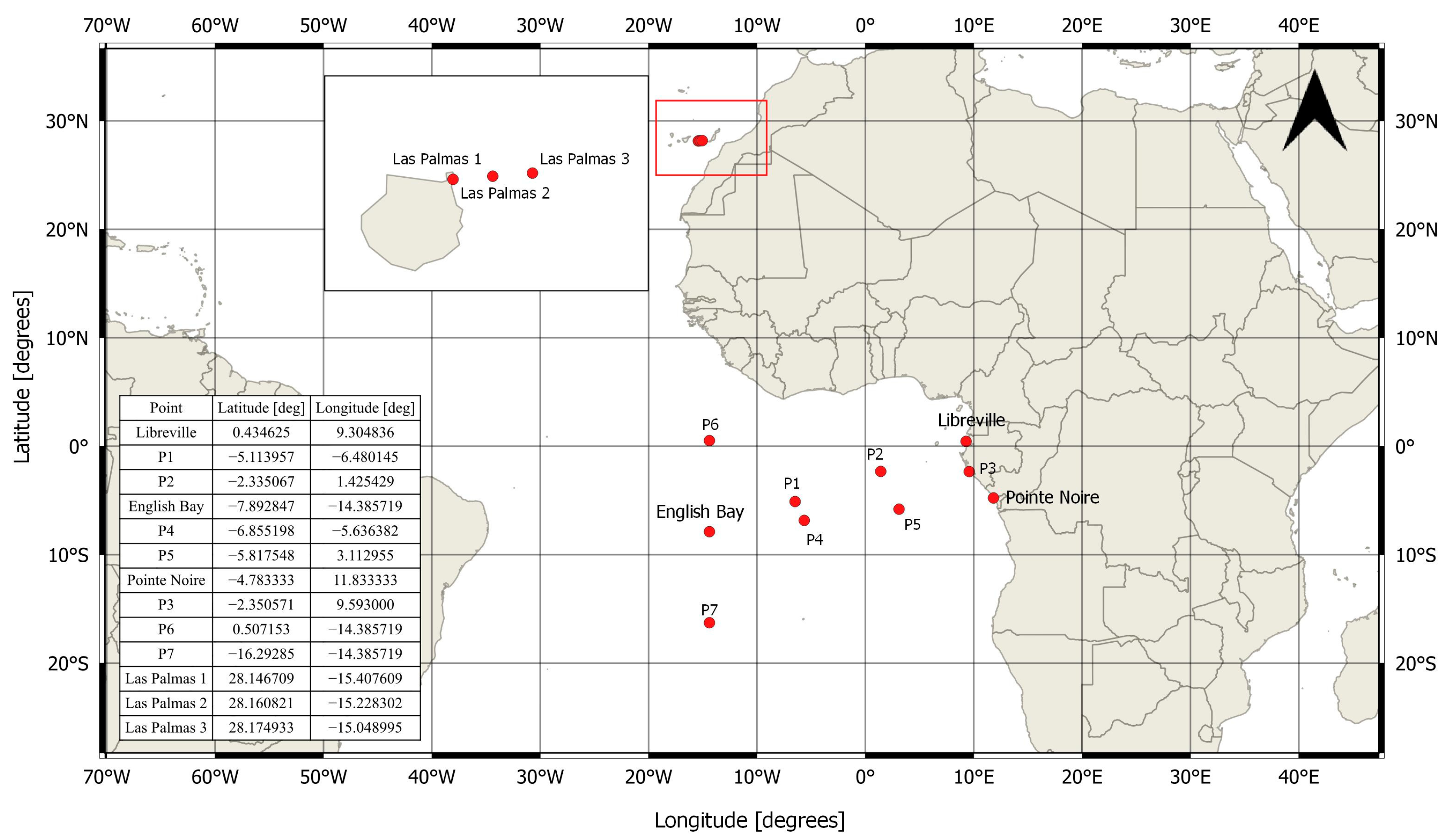
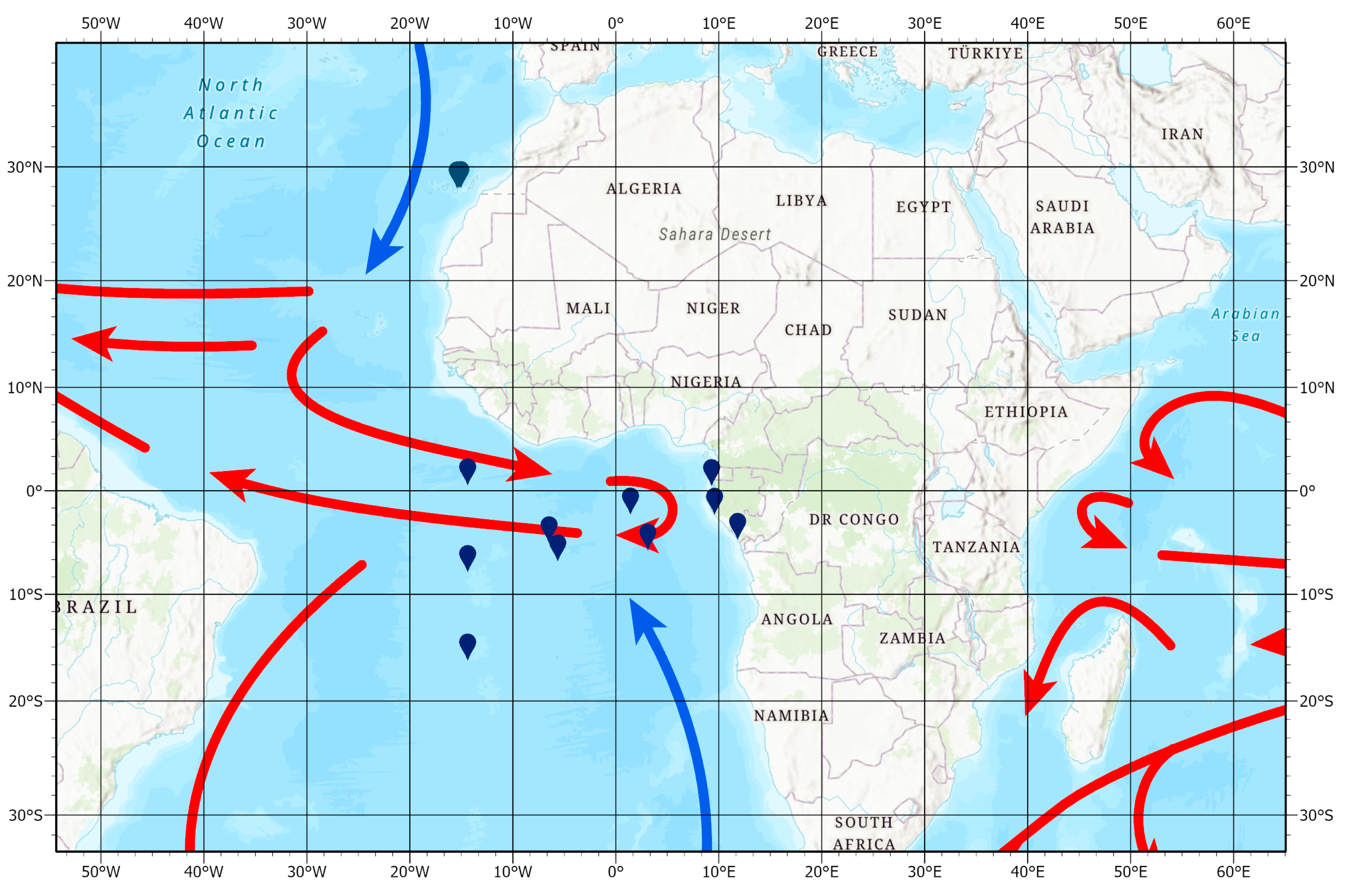
2.1. Study Sites

In this study, an investigation of the relationship between observations from satellite altimetry and bathymetry was carried out in the western part of Africa. It includes three points on the west coast—Libreville, Pointe Noire (tide gauge station), and P3. Furthermore, two tide gauge stations—English Bay (Saint Helena Island) and Las Palmas C (Canary Islands) (named Las Palmas 1)—and nine additional points, at different distances from the continent, were chosen. Research points are shown in Figure 1.

2.2. Data

The study used open-access data made available by the following repositories:

• Tide gauge (TG): Permanent Service for Mean Sea Level (PSMSL) [13]—information and products used in research, related to land movements sea level rise, and variability—tide gauge data, high-frequency data, GNSS-IR Records, etc. We obtained only the coordinates of the selected tide gauge stations;
• Satellite altimetry (SA): Copernicus Marine and Environment Monitoring Service (CMEMS) [14]- service provides free, regular, and systematic authoritative information on the state of the Blue (physical), White (sea ice), and Green (biogeochemical) ocean on a global and regional scale (https://marine.copernicus.eu/ accessed on 15 May 2022). Raw data were obtained from the “SEALEVEL_GLO_PHY_L4_MY_008_047”—“GLOBAL OCEAN GRIDDED L4 SEA SURFACE HEIGHTS AND DERIVED VARIABLES REPROCESSED (1993-ONGOING)” model (https://data.marine.copernicus.eu/products?q=SEALEVEL_GLO_PHY_L4_MY_008_04 accessed on 15 May 2022). These were altimeter satellite gridded, daily Sea Level Anomalies (SLA) over a period of 29 years (01/01/1993-31/12/2021) with 0.25° × 0.25° spatial resolution;
• Bathymetry (BATH): The General Bathymetric Chart of the Oceans (GEBCO) [15]—raster terrain model in a 2° × 2° grid. This service shares a global terrain model for ocean and land, providing elevation data in meters, with a spatial resolution of 15 arc seconds (∼500 × 500 m pixel size at the equator). We used GEBCO_2022 Grid (for profile number 4,5,6) and GEBCO_2021 Grid (for profile number 1,2,3,7). The grid uses Version 2.4 and 2.2 of the SRTM15+ data set as “a base” [16]. Files can also be released as GeoTiff data and Esri ASCII rasters for areas precisely defined by the user. The data is also accompanied by a type identifier (TID) grid that contains information about the source data types. The resolution of the data distributed by GEBCO gives reliable accuracy compared to other files of this type. In addition, the service is constantly working to improve its datasets to provide the most reliable, publicly available bathymetric grids for the world’s oceans.

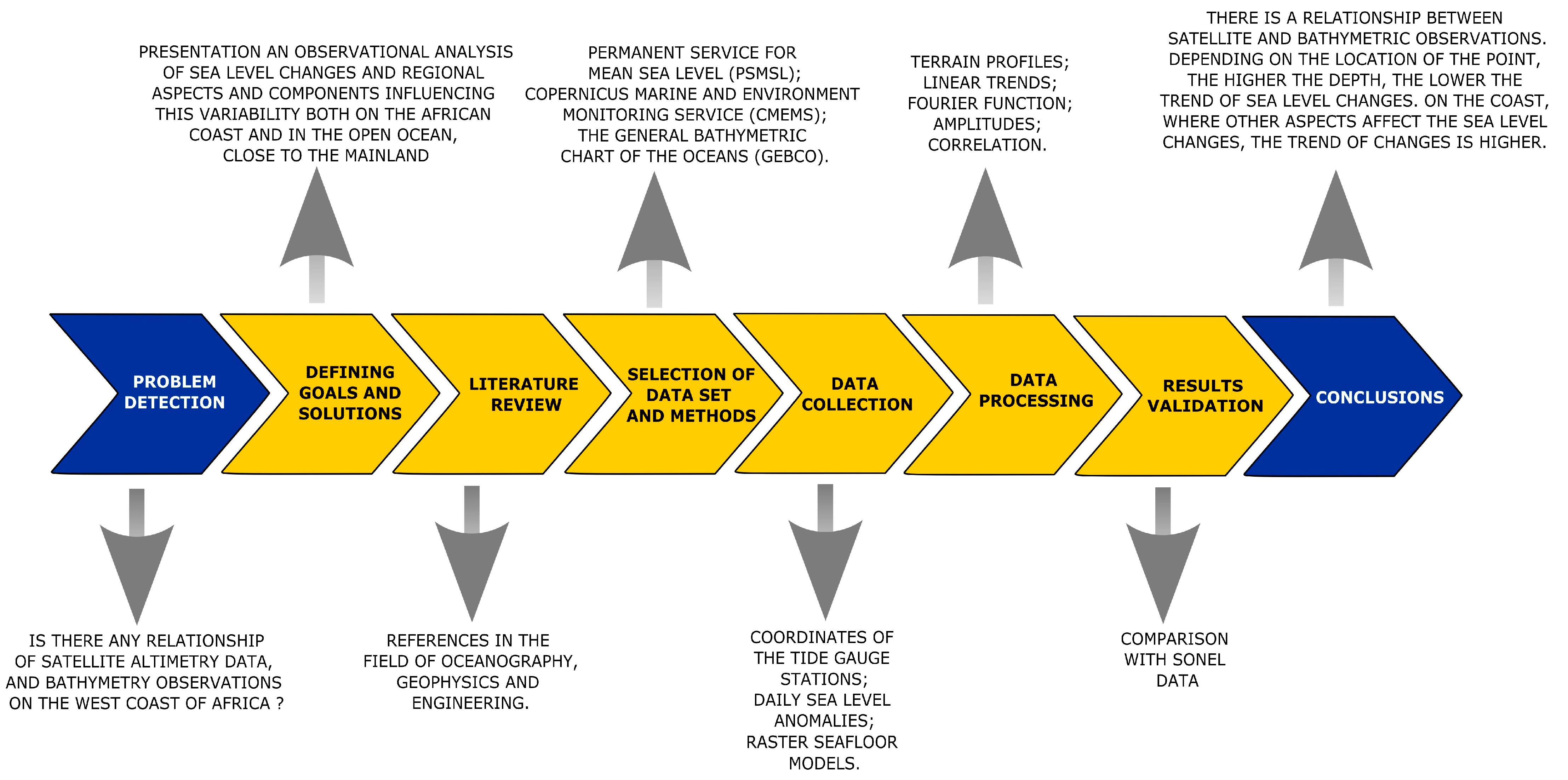
2.3. Methodology

The research includes an analysis of the velocities of changes in sea level, water temperature, and salinity. The next step is to determine the correlation between determined trends and elevation, based on bathymetric models, in terms of relationships between sea level changes and influencing factors, e.g., sea topography. The following approaches were used:

• Determination of intermediate points (P1, P2, P3, P4, P5, P6, P7, Las Palmas 2, Las Palmas 3);
  The intermediate points were determined based on a grid analysis of the tide gauge (at selected coastal points) and altimetric data nodes, so the distance intervals were close. Spatial data analysis software was used. Coordinates of the points were generated in the World Geodetic System 1984 (WGS 84).
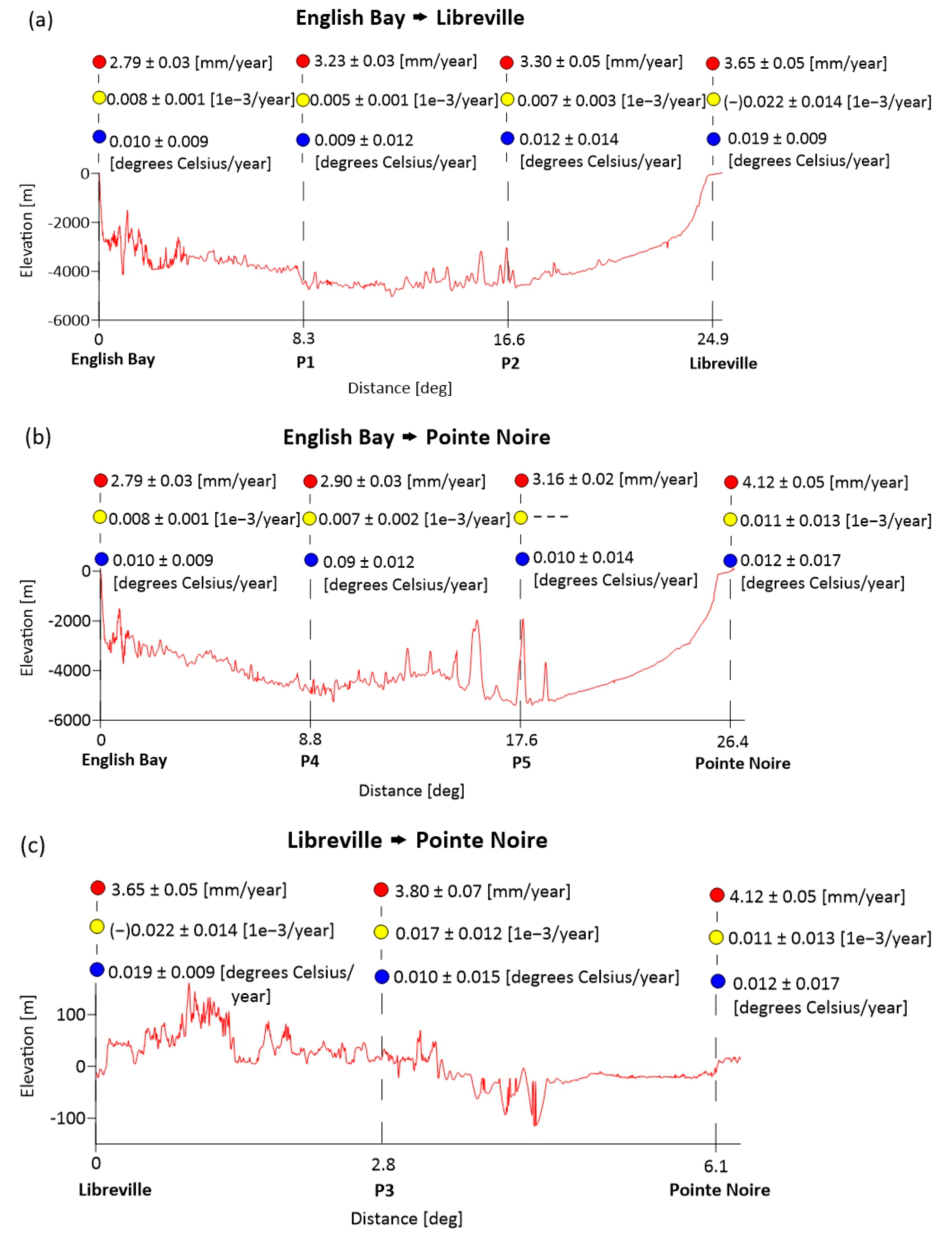
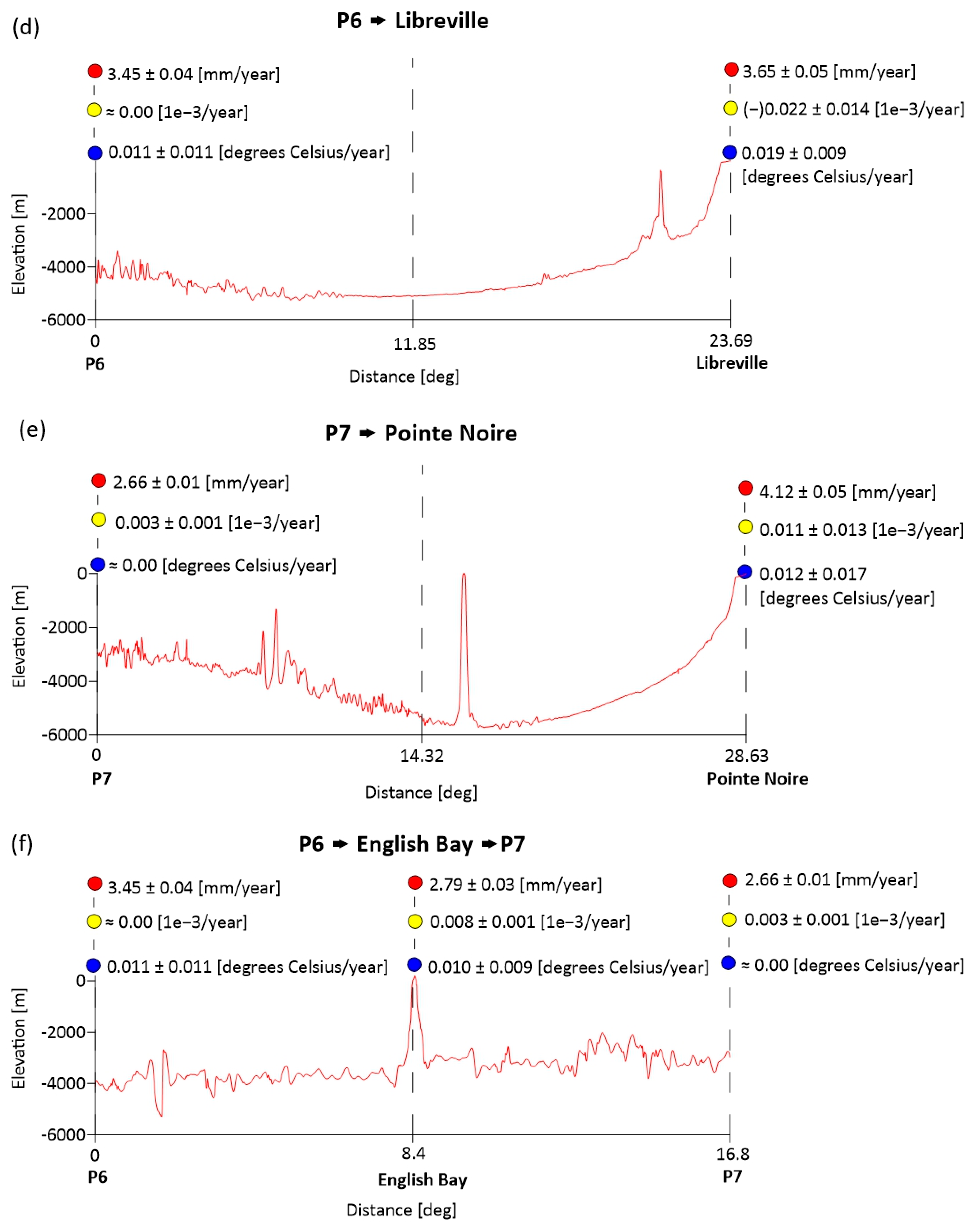
• Generation of field profiles:
  Terrain profiles were generated using specialized Surfer software, based on bathymetric model grids, provided by GEBCO from combinatorial surveys such as 40 (Predicted based on satellite-derived gravity data—depth value is an interpolated value guided by satellite-derived gravity data) and 11 (Multibeam—depth value collected by a multibeam echo-sounder). Vertical intersection with linear interpolation was used. The profiles were generated in a uniform WGS84 system.
  • Profile 1: English Bay→P1→P2→Libreville;
  • Profile 2: English Bay→P4→P5→Pointe Noire;
  • Profile 3: Libreville→P3→Pointe Noire;
  • Profile 4: P6→Libreville;
  • Profile 5: P7→Pointe Noire;
  • Profile 6: P6→English Bay→P7;
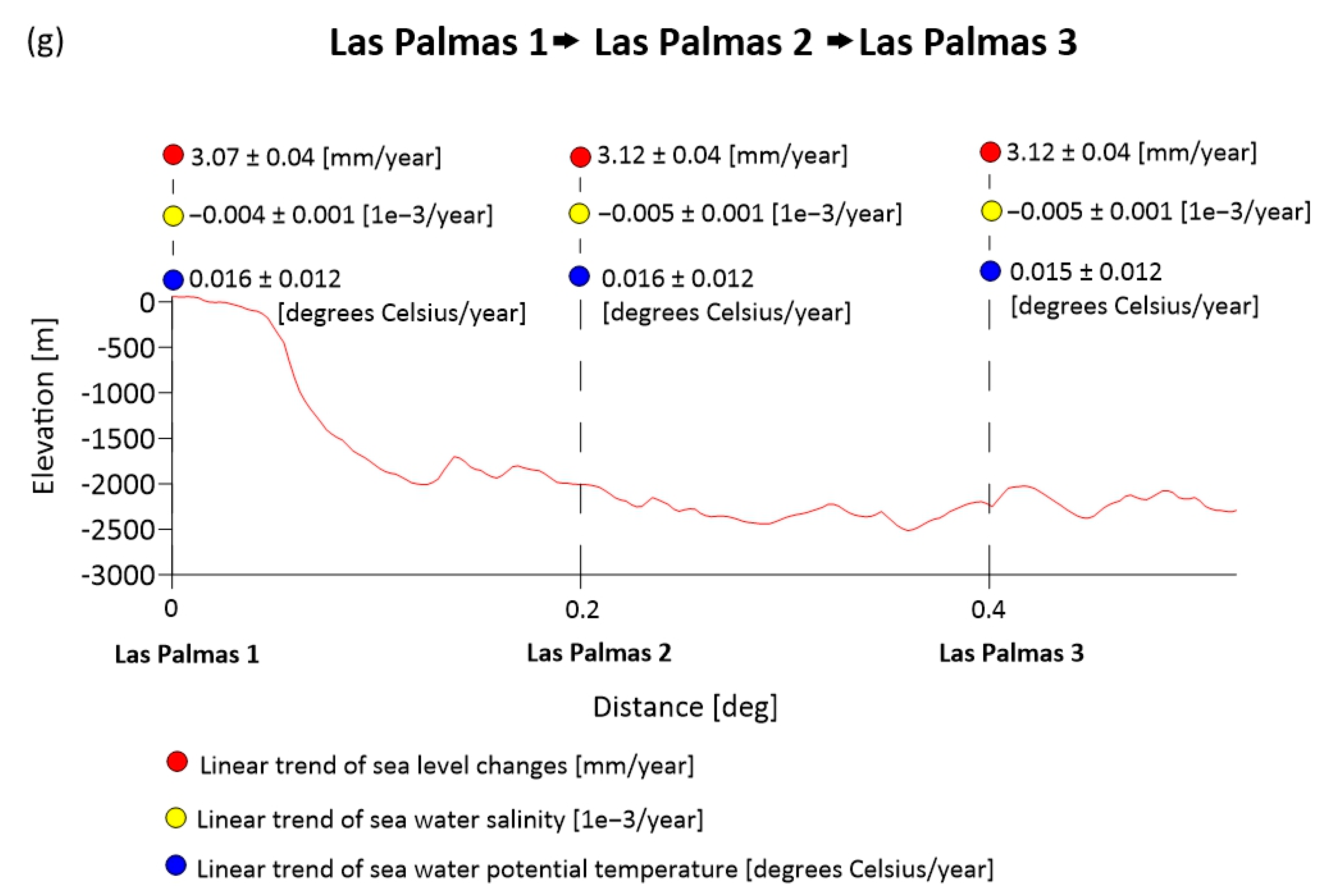
  • Profile 7: Las Palmas 1 → Las Palmas 2 → Las Palmas 3.
• Estimating the linear trend for Sea Level Anomaly (SLA) time series;
  From altimetric data, time series with a uniform interval in weekly epochs were created. Linear trend estimation was performed using the linear regression method over the full available range of SLA data. The time series was verified for vertical jumps, and their corrections were made. SLA time series without a linear trend were subjected to seasonality analysis.
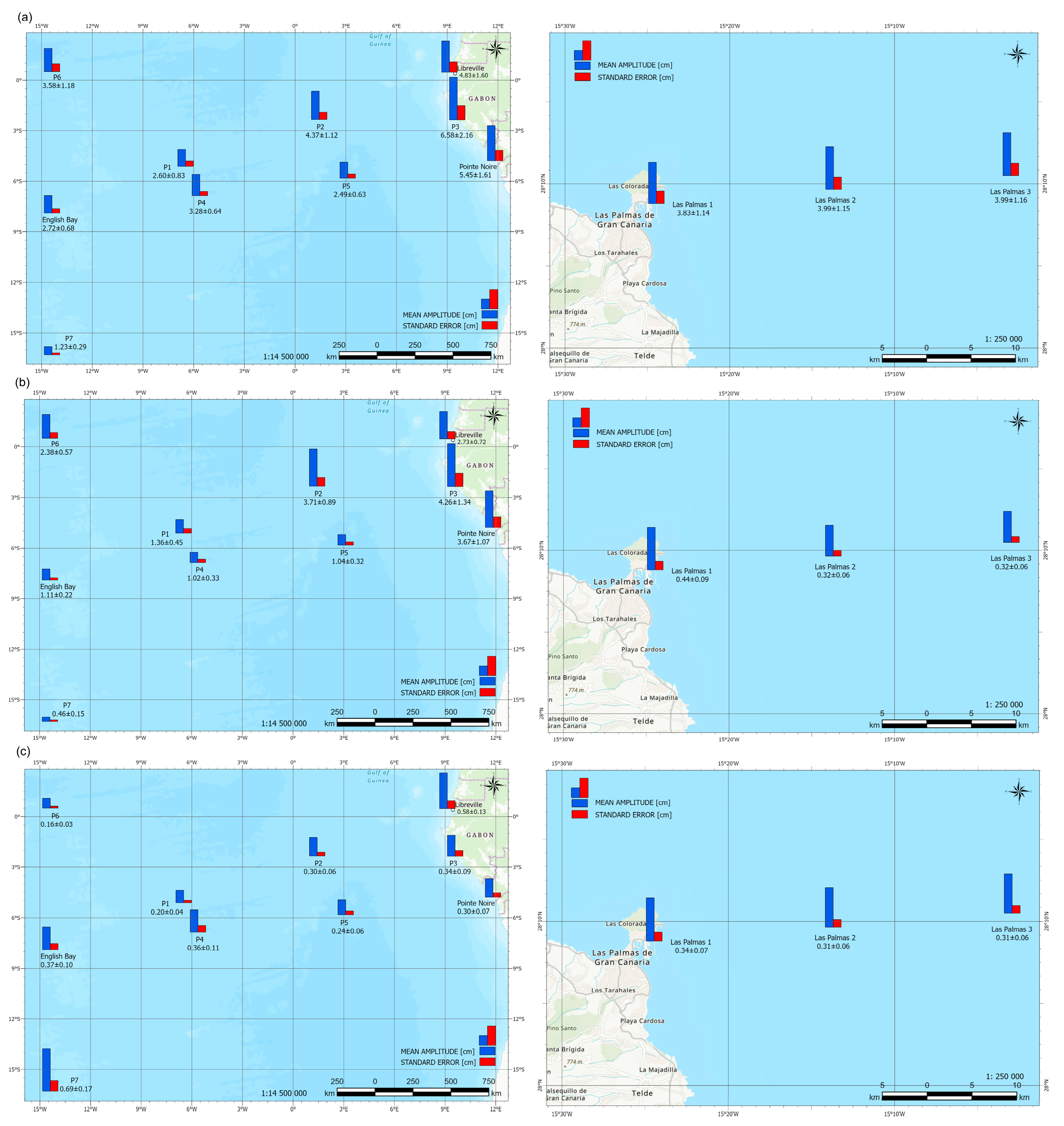
• Estimating the annual, semi-annual, and 18.61-year amplitudes of the Moon’s Nodal Cycle to remove seasonality from the time series;
  In order to estimate amplitudes, linear trends were removed from the time series. The reduced time series were analyzed for the values of amplitudes at fixed standard and non-standard periods. Amplitudes were determined using the harmonics model method based on sine and cosine functions. Based on the above analyses, annual, semi-annual, and 18.6-year seasonality were removed from the time series.
• Estimating the trend of sea water salinity and the trend of sea water potential temperature;
  The trend of sea water salinity and the trend of sea water potential temperature were estimated at points in each profile. The created time series, based on the data obtained from satellite altimetry, was subjected to a purging procedure. The time series was verified for vertical jumps, and their corrections were made. The trend was estimated using the linear regression method. The standard errors were calculated for each trend.
• Determining the trend of sea level changes using the Fourier function;
  Based on the structured time series, the trend was estimated using Fourier analysis over the full range of SLA data. This procedure uses the analysis of seasonal components (annual, semi-annual, and 18.61-year cycles), and it can be expressed as follows:

  $$f_F\left(t\right)=a+bt+A_{a}cos \left({\omega }_{a}t-{\phi }_a\right)+A_{sa}cos \left({\omega }_{sa}t-{\phi }_{sa}\right)+A_{18.61}cos \left({\omega }_{18.61}t-{\phi }_{18.61}\right)$$

  (1)

  where f_F(t) is a Fourier function; a is the bias; b is the trend; t is time; A_a and A_sa are the annual and semi-annual amplitudes; φ_a and φ_sa are the annual and semi-annual phase; ω_a and ω_sa are the annual and semi-annual angular frequency. A_18.61 is the 18.61-year amplitude; φ_18.61 is the 18.61-year phase; ω_18.61 is the 18.61-year angular frequency [17].

As a result, the value of the long-term trend and the error of its determination were obtained.

vii.

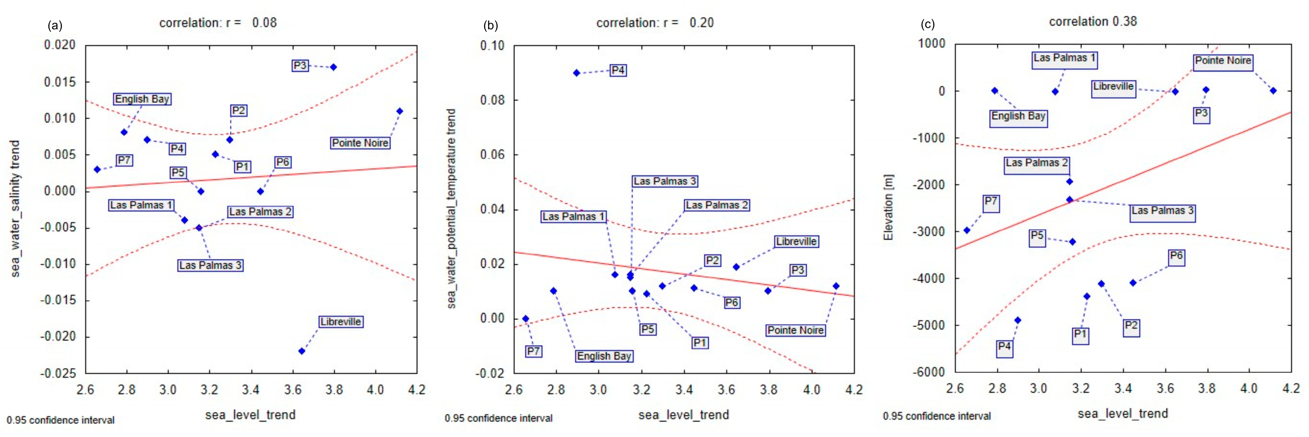
Estimating the correlation between the sea level trends, sea water potential temperature trends, sea water salinity trends (based on satellite altimetry data), and elevation from bathymetric data.

The correlation analysis was based on trends determined for the three types of data at each point. Statistics software was used to determine the simple linear correlation of the time series. The correlation assessment took into account the ratio of the trend determination error to the trend value. Pearson’s correlation coefficients (r) were calculated based on the method of covariance.

A flow chart of the study process is presented in Figure 2.

3. Results and Discussion

Linear trends in selected stations were estimated from different time series of satellite altimetry data (from January 1993 to December 2021). Changes in sea level, sea water salinity, and sea water potential temperature are presented in Figure 3.

In this study, as a result of the determination of the velocity of changes, the trends are not always coherent, the values in different locations show significant differences—they deviate from the global value. An example is a P6 point north of the English Bay station, where the trend is 3.45 ± 0.04 mm·year⁻¹.

On the other hand, to the south, at point P7, the trend is definitely lower and amounts to 2.66 ± 0.01 mm·year⁻¹. At Saint Helena Island, the trend at English Bay station is 2.79 ± 0.03 mm·year⁻¹. Along the coast, at points, Libreville, P3, and Pointe Noire trends are higher (average 3.86 mm·year⁻¹). At intermediate points, located in the open sea, P1, P2, P4, and P5 trends are approaching the global sea level (3.15 mm·year⁻¹ on average). Similarly, for points located in the Canary Islands (Las Palmas 1, Las Palmas 2, Las Palmas 3), trends do not deviate from the global value (about 3.10 mm·year⁻¹). All the points selected for the study are located in the area of 30–30°S, where ocean currents (shown in Figure 4) and constant trade winds (shown in Figure 5) can have a significant impact.

The study indicates that, from 1993 to 2020, the temperature trend at the assessed points is, on average, 0.018 ± 0.012 °C year⁻¹. At almost all locations, the trend of sea water potential temperature is positive. It adopts the highest values for the Libreville point and the Las Palmas points. Only at point P7 is the value around 0 °C. Temperature fluctuations in the upper layers are associated with heat exchange with the atmosphere and surrounding ocean regions, while temperature in the deeper parts of the oceans changes due to dynamic forcing mechanisms, such as climate change. The analysis shows an average salinity trend of 0.008  ±  0.005 1e⁻³ year⁻¹. The highest values occur at the P3 and Pointe Noire points. At points P6 and P7, the values are very close to 0 1e⁻³ year⁻¹. The three points of Las Palmas are, on average, −0.004 ± 0.001 1e⁻³ year⁻¹. It can be caused by the location in the area of the islands or the phenomenon of upwelling. At the Libreville point, the salinity trend is also negative, which could be due to the influx of freshwater from the continent. Using the time series, using Fourier analysis at each point, annual, semi-annual, and 18.61-year amplitudes were determined. Received results are presented below:

Annual amplitudes (Figure 6a) take the highest values for coastal points—Libreville, P3, Pointe Noire, and P2 (for 4.37 ± 1.12 cm to 6.58 ± 2.16 cm). The lowest value occurs at point P7(1.23 ± 0.29 cm). In the Las Palmas area, the amplitudes are at the level of 3.94 ± 1.15 cm. At the other points, the values oscillate within the limits of 2.49 ± 0.63 cm to 3.58 ± 1.18 cm. Semi-annual amplitudes (Figure 6b) take the highest values for Libreville (0.58 ± 0.13 cm) and P7 (0.69 ± 0.17 cm). The lowest value occurs at the point P6 (0.16 ± 0.03 cm). In the Las Palmas area, the amplitudes are at the level of 0.36 ± 0.07 cm. At the other points, the values oscillate within the limits of 0.20 ± 0.04 cm to 0.37 ± 0.10 cm. The 18.61-year lunar nodal cycle amplitudes (Figure 6c) take the highest values for coastal points—Libreville, P3, Pointe Noire, and P2 (for 2.73 ± 0.72 cm to 4.26 ± 1.34 cm). The lowest value occurs at point P7 (0.46 ± 0.15 cm). In the Las Palmas area, the amplitudes are at the level of 0.32 ± 0.06 cm. At the other points, the values oscillate within the limits of 1.02 ± 0.33 cm to 2.38 ± 0.57 cm.

The final step of the study was to determine the linear relationship, through correlation coefficients, between the trends identified earlier and the elevation of the terrain at all points. The results obtained were presented in Figure 7.

The linear correlation coefficient determination is the first and necessary step to establish a functional relationship between two variables. The analysis indicates very small values. The correlation coefficients for the sea water temperature trend and the sea water salinity trend—determined at 0.20 and 0.08—present a weak linear relationship. The correlation coefficients are so low because the standard errors of salinity trend and sea water temperature trend are low and, hence, the confidence in the determined trends is insufficient. Correlation takes a slightly higher value for elevation, which was determined at 0.38. For many research tasks, being based on the correlation coefficient could be inadequate, and it is necessary to use other indicators of statistical association.

The variability of results can also be affected by winds. The study area is located in the trade winds zone. According to Copernicus Ocean State Report [18], the tropical regions have the most extreme surface wind speeds, regularly reaching speeds above 250 km/h⁻¹ (70 ms⁻¹). Moreover, the 99th percentile wind speeds range from, at minimum, below 10 ms⁻¹ at the equator to local maximum values exceeding 25 ms⁻¹ in the northern Atlantic Ocean [18]. The Menendez [2] analysis presents the spatial distribution of months with the highest probability of a high-water level value. In northern Africa and the Las Palmas area, a pronounced rise in sea level occurs in the autumn months (September–November), while in the south of the continent, the highest rise occurs in the summer months. However, it was indicated that the results are affected by local factors, such as river runoff. Our study in the Las Palmas region indicates the highest sea level anomalies in October (positive) and in April (negative). In coastal points (Libreville, P3, Pointe Noire), the highest sea level anomalies occur in December/January (positive) and in July (negative). In points P1 and P7, the highest sea level anomalies occur in April (positive) and in October (negative). In points P2 and P3, the highest sea level anomalies occur in December/January/February (positive) and in July (negative). The highest positive sea level anomalies at the other points are as follows: P4 (May), P5 (March), and English Bay (June). The highest negative sea level anomalies at the points are as follows: P4 (November), P5 (September), and English Bay (December). The global sea surface temperature warmed, from 1993 to 2015, at a rate of 0.016 ± 0.002 °C/year⁻¹ [19]. The warm temperature conditions during 2016, at the sea surface, are consistent with the subsurface temperature trend over the 1993–2016 period [1]. Our results do not diverge from the global value, and the achieved average temperature is 0.018 ±  0.012 °C/year⁻¹.

According to Kennedy 2014 [20], an important factor that can affect the variability of sea surface temperature (SST) is the El Niño Southern Oscillation (ENSO), which temporarily increases global SST, as well as La Niña, which decreases it [20].

Sea surface salinity is important primarily because of its relationship to changes in the Earth’s hydrological cycle [21,22] and ocean dynamics [23]. In our study, the average salinity trend is 0.008 ± 0.005 1e⁻³ year⁻¹, while only in the Las Palmas and Libreville points, the salinity trend assumes negative values. Global subsurface salinity changes in 2016 prevail in the upper 200 m depth layers.

The surface salinity trend over the period of 1993–2016 shows enhanced values in the western Pacific warm pool areas in both hemispheres. A positive trend is manifested in the North Atlantic western boundary current regime.

Movements of the earth’s crust are also associated with changes in sea level [24,25,26], which are manifested by the vertical and horizontal displacement of tectonic plates [27]. In our work, we also checked the absolute movements of the earth’s crust (geocentric), which are determined on the basis of direct GNSS measurements and combined measurements from mareographs and satellite altimetry [28].

There were two GNSS stations selected and available in the study area, and they were located in Saint Helena and Gran Canaria, as well as in the Libreville area of Gabon.

The condition was the proximity of the available tide gauge stations [29,30]. We analyzed the movement of the earth’s crust determined from the combination of TG (tide gauge) and SA (satellite altimetry) data [17]. SA and TG time series currently represent the two main sources of information for the sea level [31]. TG observations reflect the local variations in sea level, and they are influenced by the VLM effect and the coastal processes differently from the SA records that provide geocentric sea level variations. SA and TG data sets are, moreover, characterized by low and high acquisition rates, respectively [31,32,33]. The result of the analysis was used to calculate linear trends in vertical crust movement out of the TG sites in Ascension Island, Gran Canaria, and Libreville/Gabon, based on SA data minus TG data. Velocities of crust movement calculated in this study, SA–TG, are based on GNSS data from SONEL network data calculated by different analytical centers [34]. The results obtained were presented in

Table 1. Velocities of crust movement calculated in this study are based on GNSS data and SONEL network data calculated by three analytical centers (ULR, NGL, JPL). The last column presents the sea level differences from time series of satellite altimetry minus tide gauge from SONEL network.

Analysis Centre	ULR	JPL	NGL	In Work	SONEL
Reference Frame, Ellipsoid	ITRF08, GRS80	ITRF14, GRS80	ITRF14, GRS80	SA-TG	SA-TG
GNSS Station	Velocity ± Standard Error [mm·year−1]	Velocity ± Standard Error [mm·year−1]	Velocity ± Standard Error [mm·year−1]	Velocity ± Standard Error [mm·year−1]	Velocity ± Standard Error [mm·year−1]
ASC1 (Ascension Island)	−0.37 ± 0.30 (2000–2007)	-	-	0.79 ± 0.32 (1993–2018)	-
ASCG (Ascension Island)	0.21 ± 0.26 (2015–2021)	-	−0.63 ± 0.81 (2015–2022)	0.79 ± 0.32 (1993–2018)	-
ULP2 (Gran Canaria)	-	-	−1.15 ± 1.08 (2018–2022)	−2.10 ± 1.52 (1993–2021)	−0.68 ± 0.16 (1993–2014)
PLUZ (Gran Canaria)	−1.92 ± 0.17 (2004–2013)	-	-	−2.10 ± 1.52 (1993–2021)	-
NKLG (Gabon)	−0.51 ± 0.34	−1.33 ± 0.57	-	-

.

As you can see, there are movements of the earth’s crust in selected locations. The results obtained during our research of vertical movement velocity were different with the result from SONEL network. Differences in values may be connected with the different length of the time series and chosen time periods.

4. Conclusions

The sea level averaged in time and space (i.e., excluding waves, tides, etc.), and these changes, together with the knowledge of the topography of the ocean floor, inform us indirectly about the volume of the entire ocean of water. The variation in sea level changes also depends on the changes in water mass, and the mass depends not only on the volume but also on the temperature and salinity level [35].

The actual shape of the ocean’s surface is additionally diversified by such phenomena as tides, differences in atmospheric pressure, wind patterns, the thermal expansion of water, or ocean circulation phases [36]. The presented results on our models show that the topography correlates with changes in the height of the sea surface. This relationship does not apply to the coastal points—Libreville, P3, and Pointe Noire.

Depending on the location of the point, the higher the depth, the lower the trend of the sea level changes. On the coast, where other aspects affect the sea level changes, the trend of changes is higher. The highest trends of sea level changes occur in point P6 and at coastal points (Libreville, P3, Pointe Noire). These points cover the direction of the warm Guinea Current. The lowest trend values occur in points away from the coast—English Bay, P4, and P7. The reason may be the location of the points between the warm Brazil Current and the cold Benguela Current. Research shows that there is a relationship between satellite and bathymetric observations on the west coast of Africa. Sea level is the surface of the ocean where water meets air, and the ocean floor is where water meets the earth’s crust. This is influenced by the parameters on which changes in sea level depend.

References

1. Von Schuckmann, K.; Le Traon, P.Y. Copernicus Marine Service Ocean State Report; ISSUE 2. J. Oper. Oceanogr. 2018, 11, S1–S142. [Google Scholar]
2. Menéndez, M.; Woodworth, P.L. Changes in extreme high water levels based on a quasi-global tide-gauge data set. J. Geophys. Res. Oceans 2010, 115, 7. [Google Scholar] [CrossRef] [Green Version]
3. Lan, W.-H.; Kuo, C.-Y.; Lin, L.-C.; Kao, H.-C. Annual Sea Level Amplitude Analysis over the North Pacific Ocean Coast by Ensemble Empirical Mode Decomposition Method. Remote Sens. 2021, 13, 730. [Google Scholar] [CrossRef]
4. Woodworth, P.L.; Melet, A.; Marcos, M.; Ray, R.D.; Wöppelmann, G.; Sasaki, Y.N.; Cirano, M.; Hibbert, A.; Huthnance, J.M.; Monserrat, S.; et al. Forcing factors causing sea level changes at the coast. Surv. Geophys. 2019, 40, 1351–1397. [Google Scholar] [CrossRef] [Green Version]
5. Nicholls, R.J.; Lincke, D.; Hinkel, J.; Brown, S.; Vafeidis, A.T.; Meyssignac, B.; Hanson, S.E.; Merkens, J.-L.; Fang, J. A global analysis of subsidence, relative sea-level change and coastal flood exposure. Nat. Clim. Chang. 2021, 11, 338–342. [Google Scholar] [CrossRef]
6. Allison, L.C.; Palmer, M.D.; Haigh, I.D. Projections of 21st century sea level rise for the coast of South Africa. Environ. Res. Commun. 2022, 4, 025001. [Google Scholar] [CrossRef]
7. Stammer, D.; Cazenave, A.; Ponte, R.M.; Tamisiea, M.E. Causes for Contemporary Regional Sea Level Changes. Annu. Rev. Mar. Sci. 2013, 5, 21–46. [Google Scholar] [CrossRef] [Green Version]
8. Storto, A.; Bonaduce, A.; Feng, X.; Yang, C. Steric Sea Level Changes from Ocean Reanalyses at Global and Regional Scales. Water 2019, 11, 1987. [Google Scholar] [CrossRef] [Green Version]
9. Pawlowicz, R. Key Physical Variables in the Ocean: Temperature, Salinity, and Density. Nat. Educ. Knowl. 2013, 4, 13. [Google Scholar]
10. Reagan, J.R.; Zweng, M.M.; Seidov, D.; Boyer, T.P.; Locarnini, R.A.; Mishonov, A.V.; Baranova, O.K.; Garcia, H.E.; Weathers, K.W.; Paver, C.R.; et al. Volume 6: Conductivity. In World Ocean Atlas 2018; NOAA Atlas NESDIS 86; A. Mis-honov Technical Editor; 2019; p. 38. Available online: https://www.ncei.noaa.gov/sites/default/files/2021-03/WOA18_Vol6_Conductivity%20%281%29.pdf (accessed on 12 December 2021).
11. Avşar, N.; Kutoğlu, H. Recent Sea Level Change in the Black Sea from Satellite Altimetry and Tide Gauge Observations. ISPRS Int. J. Geo-Inf. 2020, 9, 185. [Google Scholar] [CrossRef] [Green Version]
12. Taqi, A.M.; Al-Subhi, A.M.; Alsaafani, M.A.; Abdulla, C.P. Improving Sea Level Anomaly Precision from Satellite Altimetry Using Parameter Correction in the Red Sea. Remote Sens. 2020, 12, 764. [Google Scholar] [CrossRef] [Green Version]
13. PSMSL. Available online: https://www.psmsl.org/ (accessed on 12 December 2021).
14. CMEMS. Available online: https://data.marine.copernicus.eu/products (accessed on 15 May 2022).
15. GEBCO. Available online: https://www.gebco.net/data_and_products/gridded_bathymetry_data/ (accessed on 14 June 2022).
16. Tozer, B.; Sandwell, D.T.; Smith, W.H.F.; Olson, C.; Beale, J.R.; Wessel, P. Global Bathymetry and Topography at 15 Arc Sec: SRTM15+. Earth Space Sci. 2019, 6, 1847–1864. [Google Scholar] [CrossRef]
17. Kowalczyk, K.; Pajak, K.; Wieczorek, B.; Naumowicz, B. An Analysis of Vertical Crustal Movements along the European Coast from Satellite Altimetry, Tide Gauge, GNSS and Radar Interferometry. Remote Sens. 2021, 13, 2173. [Google Scholar] [CrossRef]
18. Terms, F. Copernicus Ocean State Report; Issue 6. J. Oper. Oceanogr. 2022, 15, 1–220. [Google Scholar] [CrossRef]
19. Von Schuckmann, K.; Roquet, H.; Pisano, A.; Embury, O.; Axell, S.; Balmaseda, M.; Breivik, L.; Brewin, R.; Bricaud, C.; Drevillon, M.; et al. The Copernicus Marine Envi-ronment Monitoring Service Ocean State Report. J. Oper. Oceanogr. 2016, 9 (Suppl. S2), S235–S320. [Google Scholar] [CrossRef]
20. Kennedy, J.J. A review of uncertainty in in situ measurements and data sets of sea surface temperature. Rev. Geophys. 2014, 52, 1–32. [Google Scholar] [CrossRef]
21. Curry, R.; Dickson, B.; Yashayaev, I. A change in the freshwater balance of the Atlantic Ocean over the past four decades. Nature 2003, 426, 826–829. [Google Scholar] [CrossRef]
22. Durack, P.J. Ocean Salinity and the Global Water Cycle. Oceanography 2015, 28, 20–31. [Google Scholar] [CrossRef] [Green Version]
23. O’Kane, T.J.; Monselesan, D.P.; Maes, C. On the stability and spatiotemporal variance distribution of salinity in the upper ocean. J. Geophys. Res. Oceans 2016, 121, 4128–4148. [Google Scholar] [CrossRef]
24. Billiris, H.; Paradissis, D.; Veis, G.; England, P.; Featherstone, W.; Parsons, B.; Cross, P.; Rands, P.; Rayson, M.; Sellers, P.; et al. Geodetic determination of tectonic deformation in central Greece from 1900 to 1988. Nature 1991, 350, 124–129. [Google Scholar] [CrossRef]
25. Blewitt, G.; Altamimi, Z.; Davis, J.; Gross, R.; Kuo, C.-Y.; Lemoine, F.G.; Moore, A.W.; Neilan, R.E.; Plag, H.-P.; Rothacher, M.; et al. Geodetic Observations and Global Reference Frame Contributions to Understanding Sea-Level Rise and Variability. In Understanding Sea-Level Rise and Variability, 1st ed.; Church, J.A., Woodworth, P.L., Aarup, T., Wilson, W.S., Eds.; Blackwell Publishing Ltd.: Hoboken, NJ, USA, 2010. [Google Scholar] [CrossRef] [Green Version]
26. Douglas, B.C. Global sea level rise. J. Geophys. Res. Atmos. 1991, 96, 6981–6992. [Google Scholar] [CrossRef]
27. Cuffaro, M.; Carminati, E.; Doglioni, C. Horizontal versus vertical plate motions. eEarth Discuss. 2006, 1, 63–80. [Google Scholar] [CrossRef]
28. Wöppelmann, G.; Marcos, M. Vertical land motion as a key to understanding sea level change and variability. Rev. Geophys. 2016, 54, 64–92. [Google Scholar] [CrossRef] [Green Version]
29. Bitharis, S.; Ampatzidis, D.; Pikridas, C.; Fotiou, A.; Rossikopoulos, D.; Schuh, H. The Role of GNSS Vertical Velocities to Correct Estimates of Sea Level Rise from Tide Gauge Measurements in Greece. Mar. Geod. 2017, 40, 297–314. [Google Scholar] [CrossRef]
30. Grgić, M.; Nerem, R.S.; Bašić, T. Absolute Sea Level Surface Modeling for the Mediterranean from Satellite Altimeter and Tide Gauge Measurements. Mar. Geod. 2017, 40, 239–258. [Google Scholar] [CrossRef]
31. Meli, M.; Olivieri, M.; Romagnoli, C. Sea-Level Change along the Emilia-Romagna Coast from Tide Gauge and Satellite Altimetry. Remote Sens. 2020, 13, 97. [Google Scholar] [CrossRef]
32. Cipollini, P.; Calafat, F.M.; Jevrejeva, S.; Melet, A.; Prandi, P. Monitoring sea level in the coastal zone with satellite altimetry and tide gauges. Surv. Geophys. 2017, 38, 33–57. [Google Scholar] [CrossRef] [Green Version]
33. Picco, P.; Vignudelli, S.; Repetti, L. A Comparison between Coastal Altimetry Data and Tidal Gauge Measurements in the Gulf of Genoa (NW Mediterranean Sea). J. Mar. Sci. Eng. 2020, 8, 862. [Google Scholar] [CrossRef]
34. SONEL. Available online: https://www.sonel.org (accessed on 15 September 2022).
35. Uebbing, B.; Kusche, J.; Rietbroek, R.; Landerer, F.W. Processing Choices Affect Ocean Mass Estimates From GRACE. J. Geophys. Res. Oceans 2019, 124, 1029–1044. [Google Scholar] [CrossRef]
36. Domingues, C.M.; Centre, N.; Content, O. Global Sea Level Budget 1993–Present. Earth Syst. Sci. Data Discuss. 2018, 10, 1551–1590. [Google Scholar] [CrossRef]
Figure 1. The location of observation points, which were used to determine the relationship between satellite altimetry and bathymetry data.
Jmse 11 00149 g001
Figure 2. Flow chart of the study process.
Jmse 11 00149 g002
Figure 3. Generated seafloor models with estimated linear trends. The trend of sea level changes is visualized by red dots. The trend of sea water salinity is visualized by yellow dots. The trend of sea water potential temperature is visualized by blue dots. Seabed elevation is visualized by the red line.
Jmse 11 00149 g003aJmse 11 00149 g003bJmse 11 00149 g003c
Figure 4. Ocean currents and research points. The red arrows represent warm currents, and the blue arrows represent cold currents. The ocean currents layer was compiled from the NOAA National Weather Service and the US Army and shared as an ESRI product. This data is free for personal and educational use only. Source: (a). https://www.arcgis.com/home/item.html?id=24bfd85e97b042948e6ed4928dc45a8b (accessed on 8 November 2022); (b). https://services1.arcgis.com/VAI453sU9tG9rSmh/ArcGIS/rest/services/WorldGeo_Physical_Climate_features/FeatureServer/8 (accessed on 8 November 2022).
Jmse 11 00149 g004
Figure 5. The global extreme wind climatology map. Source: Copernicus Ocean State Report, issue 6, Journal of Operational Oceanography (2022).
Jmse 11 00149 g005
Figure 6. (a) Annual, (b) semi-annual, and (c) 18.61-year amplitudes of the seasonal cycle, based on satellite altimetry time series, in selected points. The amplitude units are centimeters.
Jmse 11 00149 g006
Figure 7. The correlation coefficients for (a) sea level trend and sea water salinity trend, as well as (b) sea level trend and sea water potential temperature trend and (c) sea level trend and elevation of the terrain. Blue rhombs-dispersion plot; area marked by red dashed lines—95% confidence interval of the regression line.
Jmse 11 00149 g007