Article

Improving the Accuracy of Seafloor Topography Inversion Based on a Variable Density and Topography Constraint Combined Modification Method

1
China Academy of Aerospace Science and Innovation, China Aerospace Science and Technology Corporation, Beijing 100176, China
2
School of Electronics and Information Engineering, Harbin Institute of Technology, Harbin 150001, China
3
Qian Xuesen Laboratory of Space Technology, China Academy of Space Technology, Beijing 100094, China
4
School of Information Science and Engineering, Harbin Institute of Technology, Weihai 264209, China
5
School of Automation, Nanjing University of Science and Technology, Nanjing 210094, China
*
Authors to whom correspondence should be addressed.
These authors contributed equally to this work.
J. Mar. Sci. Eng. 2023, 11(4), 853; https://doi.org/10.3390/jmse11040853
Submission received: 4 March 2023 / Revised: 9 April 2023 / Accepted: 12 April 2023 / Published: 18 April 2023
(This article belongs to the Special Issue Application of Altimetry in Oceanographic Research)

Abstract

:
The use of satellite altimetry to recover marine gravity anomalies allows for the rapid acquisition of seafloor topography on a wide range of regional scales. Currently, the commonly used approaches for inverting seafloor topography have been focused on the linear correlation between gravity anomalies and seafloor topography and have disregarded the effect of density contrast between the crust and seawater on depth. Therefore, we proposed a variable density and topography constraint combined modification (VDTCCM) method by deriving Parker’s formula and the Bouguer plate formula by introducing variable density and topography factors. This method can effectively recover topography-related nonlinear terms of gravity anomalies. Subsequently, the seafloor topography of the South China Sea was estimated by applying the VDTCCM method and was defined as Seafloor topography one (ST1), and following, the accuracy was evaluated using shipborne sounding data (SSD). The results indicate that the ST1 model’s SSD-checked accuracy is 23.34% and 39.42% higher than the common international models of ETOPO1 and DTU10, respectively. Moreover, the ST1 model has advantages in mapping rugged areas, showing more detailed topographical features. Consequently, the VDTCCM method can provide beneficial references for the construction of seafloor topography models on a large regional scale using gravity anomalies recovered from satellite altimetry.

1. Introduction

The seafloor’s topography is the result of the continuous evolution of global geological movements, which over time has resulted in geological features such as trenches, seamounts, and ridges. Research for underwater missile submersible platform building, the underwater navigation of submersibles, natural resource discovery, ocean wind farm construction, and the investigation of crustal plate movements requires detailed knowledge of the topography of the seafloor [1,2]. Currently, a multi-beam sonar system (MBSS) is usually mounted directly on shipboard and employed to survey the topography of abysmal seas. The MBSS works by simultaneously emitting multiple sonar beams perpendicular to the track of the vessel, which are reflected from the seafloor and received by the receiver. By recording the travel time of the sonar beams, the bathymetry is calculated based on the velocity of the sound in seawater. It is one of the main pieces of equipment for marine geological surveys and marine resource development [3]. However, mapping the global seafloor topography is costly and time-consuming due to the limitations of the platform on which it is mounted and the width of the transmitted beam. The airborne Lidar inverts the seafloor topography by simultaneously transmitting lasers at 1064 nm and 532 nm wavelengths and recording the time difference between the two laser beams. The penetration of the laser is limited if the seawater is turbid, so the technique is advantageous for detecting topography in shallow water with high accuracy [4]. In addition, the use of optical satellite imagery for the inversion of seafloor topography has the advantage of covering a wide range with high efficiency [5], but is limited by the attenuation of visible wavelengths in seawater. Therefore, topographic detection of the deep ocean is still not available using this method. New technologies are therefore urgently needed to address the rapid and accurate measurement of deep seafloor topography over large regional scales. In 1983, Dixon [6] showed through experimental analysis that marine gravity anomalies correlate with seafloor topography. This has encouraged researchers to explore the use of the gravity anomaly to estimate seafloor topography. Satellite altimetry rapidly derives marine gravity anomalies on a global scale by measuring the height of the sea surface [7]. With the development of satellite altimetry, high-precision and high-resolution marine gravity anomalies have been constructed, resulting in a global boom in scholars’ research on the inversion of seafloor topography.
At present, the main methods for the inversion of seafloor topography using marine gravity information include the SAS (Smith and Sandwell—SAS) method, the gravity-geological method (GGM), the least squares configuration, artificial intelligence, and the iterative inversion algorithm. In 1992, Smith and Sandwell designed the corresponding filter based on Parker’s algorithm [8,9], taking into account the influence of the flexural isostasy of the Earth’s crust. On this basis, they applied linear regression analysis to invert the global seafloor topography with excellent results. Fan et al. [10] used a robust estimation method to optimize the linear scale factor of the SAS method to improve the accuracy of the seafloor topography near the Sea of Japan. The GGM is based on the Bouguer plate formula, which decomposes the gravity anomaly into two parts, the regional gravity anomaly and the residual gravity anomaly, and then establishes a relationship between depth and the residual gravity anomaly [11]. It is initially applied to the prediction of bedrock depths of land and is applied to bathymetry estimation because of its simplicity and efficiency of calculation. In 2010, Kim et al. [12] successfully inverted a 2′ × 2′ seafloor topography near the Drake Passage using the gravity-geologic method. Subsequently, both Xiang et al. [13] and Sun et al. [14] improved the gravity-geologic method by optimizing the construction of the regional gravity anomalies. The optimal density difference was determined in all of these studies using an iterative method. This reduces the effect of the density contrast parameter on the inversion bathymetry, but the density contrast in the equation has lost specific physical meaning. The least squares configuration method allows for the inversion of seafloor topography by fusing multiple sources of data by constructing a covariance matrix between geoid height/gravity anomalies and bathymetry data. However, this method is computationally intensive and inefficient [15]. With the development of artificial intelligence methods, Jena et al. [16] designed a radial basis function neural network to invert the seafloor topography of the Arabian Sea according to type of geomorphology to achieve better results. Annan et al. [17] derived the relationship between the gravity anomaly, vertical gravity anomaly, vertical deviation, and seafloor topography, and proposed a convolutional neural network method. This method was used to improve the seafloor topography in the Gulf of Guinea. Wan et al. [18], based on a BP neural network with six gravity gradient tensors as inputs, inverted the seafloor topography of the Atlantic Ocean, Pacific Ocean, Indian Ocean, and Arctic Ocean, and verified the effectiveness of this method. Sun et al. [19] constructed a BP neural network model with the gravity anomaly and vertical gravity gradient anomaly as inputs, and the resulting inverse topography of the Marianas Trench was better than that of the inversion using GGM.
Fan et al. proposed an iterative inversion method based on the correlation analysis of the topography and gravity anomalies using the Oldenburg–Parker method. This method considers the influence of the higher order terms of the topography on the inversion results and achieved good results in the South China Sea [20,21]. Xu et al. [22] utilized Parker’s method to optimize the seafloor topography in the South China Sea by iteratively processing the initial results of the GGM inversion. Yu et al. [23] established the analytic observation equations for the seafloor topography and gravity anomaly, then calculated it via least-squares iteration. The root-mean-square error of the inverted seafloor topography in the South China Sea region thus reached 127.40 m.
However, the impact of variations in density contrast on inversion results has rarely been considered in seafloor topography estimation studies. As a result, the credibility of the terrain inversion results is reduced, especially when the study area is extensive. Currently, in the study of depth inversion at the Moho interface and sedimentary basins, scholars have proposed the use of variational density contrast correction and constructed various models of density contrast versus depth, including linear, polynomial, exponential, and so on [24,25,26,27]. However, we have not yet found a variable density model applied to inversion studies of seafloor topography. In fact, the density of seawater is influenced by parameters such as the temperature, salinity, and bathymetry [28], and the density of the Earth’s crust is associated with the type of material structure, depth of burial, and so on. The density contrast between the Earth’s crust and seawater varies not only horizontally, but also vertically. Therefore, the inversion of seafloor topography on a large regional scale using gravity anomalies requires consideration of changes in density contrast. Based on previous studies, we proposed a variable density and topography constraint combined modification (VDTCCM) method by deriving Parker’s forward formula and the Bouguer plate formula for the variable density. The purpose of this paper is to determine how to efficiently recover the topography-related nonlinear terms in gravity anomalies. In Section 2, the scheme for the construction of the VDTCCM method is proposed, including the deriving of the variable density Parker’s formula and the basic process of the VDTCCM method. Section 3 presents the experiments and results analysis of the seafloor topographic inversion in the South China Sea (SCS), including the correlation analysis and filtering processing of the gravity anomaly and seafloor topography, and the evaluation of the seafloor topographic inversion and accuracy. Section 4 is the conclusion of this paper.

2. Construction of the VDTCCM Method

The gravity anomaly at sea surface obtained from satellite altimetry is produced by the inhomogeneous density distribution of material below the sea surface. The seafloor topography is considered to be the shallowest density interface in the ocean. According to the interface gravity anomaly calculation method proposed by Parker, the gravity anomaly generated at sea surface by the undulations of the density interface can be quickly calculated as follows [9]:
F [ Δ g ( x , y ) ] = 2 π G ( ρ c ρ w ) e 2 π k d n = 1 ( 2 π k ) n 1 n ! F [ h n ( x , y ) ]
where F[·] denotes the Fourier transform. G is the universal gravitational constant with a value of 6.674 × 10⁻⁸ cm3/(g·s2). ρ c and ρ w are the average density of the crust and seawater, respectively. k is the radial frequency. d is the average of the seawater depth. h represents the topographic relief relative to average seawater depth with upward being positive.
The average densities of the crust and seawater are usually used in the above-mentioned forward modeling gravity anomalies using seafloor topography without sufficient consideration of those variations in the horizontal and vertical directions. We introduced a variable density model with a more realistic density contrast distribution in order to ensure the reasonableness of the forward modeling gravity anomaly results. We assumed that the density contrast varies exponentially with depth,
Δ ρ ( z ) = i = 1 N Δ ρ i e μ i z ,
where Δ ρ ( z ) is the density contrast in relation to depth. z is the absolute value of the seawater depth. Δ ρ i is the density variation parameter. μ is the density contrast attenuation coefficient. In this study, N is taken to be two according to references [27,29]. The variation parameters and attenuation coefficients in the equation can be solved using discrete density contrasts with corresponding depths using the least squares fitting method.
Subsequently, we derived the gravity anomaly forward formula for density difference with depth based on Parker’s algorithm based on the reference [30]:
F [ Δ g ( x , y ) ] = 2 π G e 2 π k d i = 1 n n = 1 ( 2 π k μ i ) n 1 n ! F [ Δ ρ i h n ( x , y ) ] ,
where the parameters in the formula are consistent with the above expression. In this paper, we take n to be two to account for the effect of the non-linear term of the terrain in the equation on the forward modeling gravity anomaly results according to reference [20].
The traditional SAS method adopts a linear regression method for the inversion of seafloor topography [8]. This ignores the effect of nonlinear factors related to topography in gravity anomalies. Therefore, in order to recover nonlinear information and consider the variation of density contrast, the inversion results are modified as follows by introducing variable density and topography constraint parameters based on the Bouguer plate formula:
h m m + 1 = h m m + ( ( Δ g o b s Δ g c a l m ) / 2 π G Δ ρ m ) ( ( h m h ¯ m ) / h ¯ m ) ,
where h m m ( m = 0 , 1 , 2 , , M ) is the medium wavelength topography corrected for m time. h m 0 represents the initial topography calculated using linear regression fitting parameters of the filtered topography and filtered gravity anomaly Δ g o b s . The Δ g o b s is the result of the gravity anomaly derived using satellite altimetry after band-pass filtering processing and downward continuation. Δ g c a l m represents the gravity anomaly calculated by Equation (3) in forward modeling for the mth correction. Δ ρ m is the variable density contrast model calculated by Equation (2). ( ( h m h ¯ m ) / h ¯ m ) is the topography constraint parameter. h m is the bathymetry result of the mth construction. h ¯ m is the mean depth of h m where the h m can be solved by the following equation:
h m = h m m + h l ,
where the h l represents the long wavelength of the seafloor topography.
When VDTCCM is used to solve the initial medium wavelength band seafloor topography, the gravity anomaly and topography are filtered according to the filter designed by Smith and Sandwell [8]. The purpose is to reduce the influence of crustal isostasy and downward continuation. Then, we determined the cutoff wavelength of the designed filter through frequency domain correlation analysis [31]. The equations for the corresponding low-pass, high-pass, and band-pass filters are as follows:
The low-pass filter:
W l = 1 1 + A k 4 e 4 π k d ,
The high-pass filter:
W h = 1 e 2 ( π k s ) 2 ,   a n d
The band-pass filter:
W = W l W h ,
where the s and A are filtering parameters, which are calculated according to reference [32]. d is the mean of the seawater depth.
The inverted seafloor topography is modified by using variable density forward modeling and a topographically constrained spatial domain. This method considers the actual situation of the density change and effectively restores the information related to topography nonlinearity in gravity anomalies. The specific process of seafloor topography inversion using the VDTCCM method is summarized as the following steps:
First, the ETOPO1 model was used to eliminate the abnormal values in the data of the shipborne sounding control points. Then, using the crustal model CRUST 1.0 and seawater density data, an empirical model of the variation of density contrast with depth in the study area was constructed according to Equation (2).
Second, the frequency domain correlation analysis was used to determine the bands of high correlation between the satellite altimetry-derived gravity anomaly and seafloor topography. We filtered the above data according to the filter designed in Equations (6) to (8).
Third, the filtered shipborne sounding control points and gravity anomalies were used to construct the initial model of medium wavelength in the seafloor topography h m 0 using the parameters of least square linear regression fitting.
Then, we completed forward modeling for the gravity anomaly of the initial seafloor topography according to Equation (3) and calculated the difference between the forward gravity anomalies and the observed gravity anomalies, Δ g o b s ; subsequently, we used Equation (4) to modify the initial seafloor topography model h m 0 .
Finally, according to Equation (5), we added the inverted seafloor topography and long-wave topography and used the removal-recovery method to fuse the shipborne sounding data to construct the seafloor topography in the experimental region.

3. Numerical Experiments and Analysis

3.1. Experimental Data and Pre-Processing

The South China Sea (SCS) is located at the junction of the Eurasian plate, the Pacific plate, and the Indo-Australian plate, which is rich in oil and gas resources. During the formation process, it experienced geological activities such as collision and subduction between plates, thus forming the northern passive type, the southern composite type, the eastern subduction active type, and the western shear type continental margin [33]. We selected the South China Sea basin (111°30′00″~118°30′00″ E, 12°30′00″~17°30′00″ N) and its surrounding areas for research (Figure 1). The eastern part of the region is the Manila Trench, formed by the subduction of the Eurasian continental plate into the Philippine plate. The area covers the Xisha Islands, the Zhongsha Trough, the Zhongsha Islands, the Zhongsha North Ridge, the Central Basin, and many seamounts of different sizes, with various geomorphic features. High-precision seafloor topography is of great significance for marine scientific research.
The data used in this study are mainly as follows:
(1)
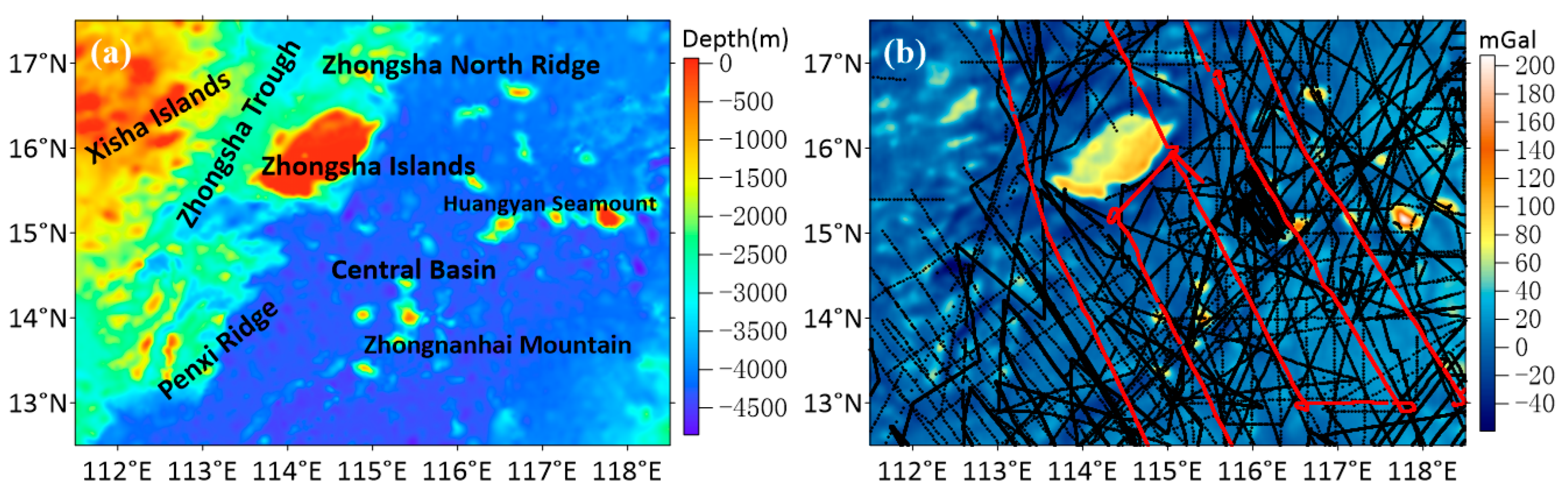
105396 shipborne sounding data (SSD) and the ETOPO1 bathymetric model [34] were obtained from the National Geophysical Data Center (NGDC) (Figure 1a). Due to the wide range and time interval of SSD collection and the difference in data processing methods, there are, inevitably, errors. Therefore, we preprocessed the SSD to ensure its quality. Then, we selected the data from track line S049 as the check points to evaluate the accuracy of the inversion seafloor topography model, as shown by the red dots in Figure 1b. The data of the remaining track lines are used as the control points for the inversion of the seafloor topography, and their distribution is shown in the black dots in Figure 1b.
(2)
The satellite altimetry-derived ocean gravity anomalies were obtained from the Scripps Institution of Oceanography (SIO). The version of the gravity anomalies is V32.1 (accessed on 2 September 2022) [35] (Figure 1b) and the resolution is 1′ × 1′.
(3)
The DTU10 seafloor topography model (accessed on 2 September 2022) [36] constructed by the Technical University of Denmark using satellite altimetry gravity data inversion was used for comparative analysis. The statistical results of the above data are shown in Table 1.

3.2. Seafloor Topography Inversion Process and Results

3.2.1. Variable Density Model Construction

The seafloor topography is the density interface between the seawater and the crust. Therefore, the gravity anomaly caused by the topographic relief is closely related to the density contrast between the crust and the seawater. The movement of seawater results in great differences in temperature and salinity in different ranges, which affects the density distribution of the seawater. In addition, plate movement and sediment differences lead to changes in crustal density. Therefore, the inversion of seafloor topography using the gravity anomaly cannot be replaced by a constant density contrast in a large area. We analyzed the seawater density model in the study area based on the theoretical formula for seawater density and the water depth data for known points and used the CRUST 1.0 model [37] (http://igppweb.ucsd.edu/~Gabi/rem.html, accessed on 12 September 2022) to extract the average density of the crust. Thus, a density contrast model of the study area was constructed to optimize the gravity anomaly of the forward seafloor topography model.
As an important marine physical parameter, seawater density is important for the study of internal ocean waves and ocean circulation. The density of seawater is closely related to its temperature, salinity, and depth. Generally, we require an instrument of Conductivity, Temperature, and Depth (CTD) to measure it. However, the density measured using this method is discrete and time-consuming. Gladkikh et al. established a theoretical density model of global seawater based on the law of seawater density changing with latitude and depth [38].
ρ D , ϕ = 1000 + α ( ϕ ) × { u ( ϕ ) + 0.5 [ 1 u ( ϕ ) ] [ 1 + tanh ( 0.00988 D 1.01613 ) ] } + β ( ϕ ) D χ ( ϕ ) ,
where the ϕ is latitude. D is the depth of the seawater in meters. α ( ϕ ) , β ( ϕ ) , χ ( ϕ ) , and u ( ϕ ) are the functions of the latitude.
α ( ϕ ) = 27.91 2.06 exp ( ( 0.0161 ϕ ) 5 )
β ( ϕ ) = 0.00637 + 0.00828 exp ( ( 0.017 ϕ ) 4.66 )
χ ( ϕ ) = 0.964 0.091 exp ( ( 0.016 ϕ ) 5 )
u ( ϕ ) = 0.928 0.079 cos ( 0.053 ϕ )
According to the CRUST 1.0 model, the 1° × 1° average crustal density model of the study area was constructed, as shown in Figure 2a. The seawater density model calculated based on Equation (9) using shipborne bathymetric data is shown in Figure 2b. The corresponding density contrast model is shown in Figure 2c.
From Figure 2a, we can see that the average density of the crust near the Xisha Islands and the Zhongsha Islands in the northwest of the study area is relatively large, which may be caused by the accumulation of a large number of various types of sediments around the continental slope near the South China Sea. However, in the Central Basin area, there are mainly deep-sea clay sediments with relatively low crustal density and gentle changes. From Figure 2b, we can see that, in the Xisha Islands area, there may be more pycnocline due to complex changes in seawater density due to the shallow depth. The change in the seawater density is stable in deep water areas such as the Central Basin. In addition, from the density contrast result Figure 2c, we can see that the density contrast between the crust and seawater is greater than 1.40 g/cm3. With the exception of the northwest and southeast of the study area, the density contrast results are basically close to the contour of the crustal density. The reason may be that the density of seawater gradually approaches a constant as the depth of the seawater increases. Therefore, the result of the density contrast is close to the result of the crustal density.
Based on the discrete density contrast model and seawater depth, the least squares method was used to fit and calculate the parameters in Equation (2). The fitted curve and model results of the density contrast are shown in Figure 3.
According to the results of the fitted curve of the density contrast in Figure 3a, the density contrasts vary from 1.525 g/cm3 to 1.650 g/cm3 within the depth range of 0–1 km. With the increase in depth, the distribution of the star points tends from discrete to relatively centralized. Therefore, the distribution law of density contrast is similar to the density of seawater, and is also affected by variations in depth. Moreover, compared with Figure 1a and Figure 3b, the density contrasts are consistent with the changes in the seafloor topography model. In the shallow area, the density contrast is large and changes sharply, while in the deep area, the density difference is relatively small and changes gently. However, due to ocean currents and seasonal variation, the seawater density presents obvious spatiotemporal changes. In this study, the factors of time change are not accounted for.

3.2.2. Seafloor Topography and Gravity Correlation Analysis and Filtering

The gravity anomalies retrieved via satellite altimetry have a strong correlation with the seafloor topography in a limited band, which is affected by the crustal isostasy and downward gravity continuation. Generally, frequency domain coherence analysis can be used to determine the band range of approximate linear correlation. We used the correlation power spectrum defined by Marks for correlation research [31]:
c o h = < F [ Δ g ( x , y ) ] ( F [ h ( x , y ) ] ) * > 2 ( < F [ Δ g ( x , y ) ] ( F [ Δ g ( x , y ) ] ) * > < F [ h ( x , y ) ] ( F [ h ( x , y ) ] ) * > ) ,
where the F represents the Fourier transform. <·> is the average value in the frequency domain. * denotes the complex conjugate. The results of the correlation coefficient between the seafloor topography and gravity anomaly calculated using Equation (13) in the frequency domain with the change of wavelength are shown in Figure 4.
From Figure 4, we can see that the gravity anomaly derived via satellite altimetry in the study area is well-correlated with the seafloor topography in the wavelength range of 25–100 km. The low correlation in the short wavelength range is mainly affected by downward continuation. The decrease in correlation in the long band range is mainly related to isostasy compensation. Therefore, in order to ensure linear correlation between the seafloor topography and gravity anomaly, the cutoff wavelength of the filter was determined to be 25 km and 100 km in Equation (6) to Equation (8), respectively. We used the filtering equation to filter the gravity anomaly and seafloor topography, respectively. The results are shown in Figure 5.
From Figure 5a,b, we can see that the gravity anomaly after band-pass filtering has a high coincidence with the seafloor topography. Especially in the seamount area of the Central Basin, there is an obvious positive gravity anomaly at the seamount. The variation of the gravity anomaly is basically consistent with the morphology of the seamounts. The filtered result of the gravity anomaly shows a negative value in the basin and trough area. In addition, the deeper the seawater depth, the lower the value of the gravity anomaly. However, the correlation between the gravity anomaly and seafloor topographic change is low near Xisha and the Zhongsha Islands. The gravity anomaly shows an archipelagic shape and is not obvious in Figure 5b. Therefore, the relationship between the gravity anomaly and seafloor topography is not completely linear. The inversion of the topography using the gravity anomaly needs to consider nonlinearity. In addition, the low-pass filtering results of the SIO 24.1 seafloor topography in Figure 5c shows the approximate contour range of the seafloor topography. The overall features of the terrain model are smoothed out and the local details are basically lost. Therefore, the medium and short wavelength of the gravity anomaly inversion of seafloor topography show more details, but the inversion results need to be supplemented by combining them with the long wavelength topography.

3.2.3. Seafloor Topographic Inversion Results

The detailed steps for the inversion of the seafloor topography using the VDTCCM method are outlined in the below flowchart Figure 6, through the construction and correlation analysis of the density contrast model described above.
First, the pre-processed discrete SSD were gridded using the Kriging interpolation. Then, the seafloor topographic grid and gravity anomalies were filtered to obtain data in different wavelength ranges. Second, bilinear interpolation was used to obtain filtered gravity anomalies and SSD at the position of the control points, respectively. Subsequently, a linear regression was fitted based on the least-squares method. The fitted parameters were also used to invert the initial seafloor topography in the medium wavelength ranges with the filtered gravity anomalies. Finally, the initial model was corrected using Equation (4) and the final seafloor topography was constructed by adding the long wavelength topography component of the SIO 24.1 seafloor topography to the corrected topography based on Equation (5). The result is shown in Figure 3a. In addition, to avoid edge effects during the inversion process, the study area was treated with a 1° outward expansion around each of its perimeters. ST1 (seafloor topography one) (Figure 7a) is the result based on the VDTCCM method. ST2 (seafloor topography two) (Figure 7b) is a model modified via constant density contrast. Figure 7c,d show the international seafloor topography models ETOPO1 and DTU10, respectively. These two international models are comparisons for the results of the inverse seafloor topography model.
From Figure 7, we can see that the four models reflect the contour pattern of the South China Sea basin with a relatively consistent SW–NE trend in the study area. In particular, the geomorphic types of the Xisha Islands, Zhongsha Islands, Zhongsha North Ridge, and Zhongnanhai Mountain are well represented, and these features are consistent with the gravity anomaly. The position is in the magenta box in Figure 7. However, the DTU10 model seems to be smoother and slightly lower in detail than the other three models. For example, in the Zhongsha North Ridge region (112°30′00″ E, 13°30′00″ N), the ST1, ST2, and ETOPO1 models reflect more high-frequency detail information compared to the DTU10 model.
Globally, the ST1 and ST2 models are similar to the ETOPO1 model in terms of terrain and geomorphological features. However, in the adjacent area of the Xisha Islands in the northwestern part of the study area, the detailed features of the ST1 and ST2 models are obviously lost due to the relatively sparse distribution of the control points. In comparison, the ST2 model behaves more smoothly. This may be related to the fact that the variation of density contrast is not considered in the model correction. Furthermore, the ST1 and ST2 models have elevated ridges in the southwest (117°48′00″ E, 13°12′00″ N), which is significantly different from the two international models. The model images of are not effective for determining the exact cause of the appearance of the ridge features here. Additional shipboard sounding data is needed to be further assessed.

3.3. Results and Discussion

The external SSD inspection data were selected for quantitative analysis of the four seafloor topography models described above. The distribution of the check data is shown as red dots in Figure 1, with a total of 12,222 shipboard measurements. The check track line is distributed in a SE–NW direction, passing through seamounts, basins, and the Zhongsha and the Xisha Islands. This is relatively objective for the results of the model accuracy assessment. Then, we used bilinear interpolation to obtain model values for each of the four models at the locations of the check data. The difference between the SSD and the model values was calculated and the statistical results are shown in Table 2. The discrete point distribution and linear regression results of the true values of the SSD and the predicted values of the models are shown in Figure 8.
From Table 2, we can see that the mean values of ST1-SSD and ST2-SSD are −13.70 m and −15.66 m, respectively. However, the mean values of ETOPO1-SSD and DTU10-SSD are −20.92 m and 58.99 m, respectively. Therefore, the ST1, ST2, and ETOPO1 models underestimate the depth, and the DTU10 model overestimates the depth compared to the check points. Nevertheless, the presence of a large number of outliers will lead to large differences in the mean values and require further determination.
In addition, the root-mean-square error (RMSE) of the difference between the model and the check data shows that ST1 has the highest accuracy (RMSE = 133.73 m), followed by ST2, ETOPO1, and DTU10, corresponding to RMSEs of 140.78 m, 174.44 m, and 220.76 m, respectively. Compared to the other three models, the accuracy of ST1 was improved by 5.01%, 23.34%, and 39.42%, respectively. It shows that the seafloor topography estimated by the VDTCCM method through the introduction of variable density contrast and topography constraints are closer to the external check data of the SSD, demonstrating the superiority of this method. However, this accuracy comparison is relative because the check data we selected are not globally uniformly distributed. This can only represent the accuracy of the model for the region of the check data distribution.
From Figure 8, the fitted correlation coefficients of the linear regression between the predicted and real depth of the models are the ST1, ST2, ETOPO1, and DTU10 models, from largest to smallest. Their values are 0.971, 0.968, 0.951, and 0.926, respectively. Among them, the R2 of the ST2 is closer to that of the ETOPO1 model than that of the ST1. However, from Figure 8c,d, the distribution of the data in the ETOPO1 and DTU10 models is more discrete than that of the ST1 and ST2. The data points of the ST1 model are concentrated and strongly correlated with the SSD, indicating that the predicted depth of ST1 is the closest to the real depth among the four models. Comparatively, the fitted result for the DTU10 model is not satisfactory. The presence of more outliers in the scatter plot indicates that the DTU10 model may have more predicted depth anomalies. Furthermore, in the range of depths from 0 to −1000 m, the predicted depths of the ST2 model are significantly lower than the real depths, as shown by the distribution of the discrete points. The distribution of scatter dots in this depth range is similar between the ST1 and ETOPO1 models. However, only a few points in this range are close to the real depth for the ETOPO1 model and the ST1. The ETOPO1 model clearly underestimates the real depth at some points. Most of the predicted points in the ST1 model overestimate the seawater depth, and the distribution of discrete points tends to be relatively concentrated as the depth increases. Therefore, the accuracy of the ST1 inversion using the VDTCCM method is affected by the depth.
To further analyze the effect of depth variation on the model accuracy, different depth layers were delineated every 1000 m, and a total of five depth variation intervals were divided. Then, the accuracy variation curve of the four models with depth was plotted, as shown in Figure 9. The results of the statistical differences between the seafloor topography models and the check data within different depth layers are shown in Table 3.
From Table 3 and Figure 9, there is an approximate trend of improving accuracy with increasing depth for all four models. In the depth range of 0~1000 m, the accuracy of all four models is not satisfactory. However, the ETOPO1 model has significantly better accuracy than the other three models, followed by the ST1, ST2, and DTU10 models. The ST1 has an accuracy of 178.22 m in the range of 1000 m to 2000 m, which is significantly superior to the other three models. At depths between 2000 m and 4000 m, the accuracy of the ST2 model is slightly better than that of the ST1 model. Notably, in the depth range above 4000 m, the accuracy of ST1 and ST2 are basically the same and obviously better than ETOPO1 and DTU10 models. Combined with Figure 3a, the rate of change of density contrast gradually decreases with increasing depth, so that ST1 and ST2 remain basically the same in the deep region. However, in the depth range from 0 to 2000 m, the rate of variability of the seawater density is larger, and the accuracy of the ST1 inverse by the VDTCCM is significantly better than that of the ST2. Therefore, it is necessary to consider the density variation of seawater in the middle and shallow areas. Meanwhile, the accuracy of the international models ETOPO1 and DTU10 is not satisfactory in shallow areas, and the RMSE of the two models reaches the minimum value in the depth range greater than 4000 m, which are 102.03 m and 175.67 m, respectively. Therefore, different inversion algorithms or depth substitutions using international models can be considered to improve the overall accuracy when inverting the seafloor topography over a large area.
To further analyze the influence of topographic variation on the accuracy of the models, three times the mean value of the RMSE of the four models’ check differences (RMSE = 510.10 m (Table 2)) was used as the standard value to evaluate the larger errors against the check data of the SSD. Points are considered as larger error dots when the absolute value of the difference between the model value and check data of the SSD is greater than the standard value. Then, the distribution of the locations of the larger error dots in each of the four models is counted and plotted separately, as shown by the red dots in Figure 10. The ST1 model has the least number of dots with 282, followed by the DTU10 model with 316. The ST2 model contains 340 large error dots. Moreover, the ETOPO1 model has the largest number of error dots with 462.
From Figure 10, we can see that there are more error dots distributed in the ST2 and DTU10 models near the Xisha Islands in the northwestern part of the study area (113°00′00″ E, 17°30′00″ N); however, the ST1 and ETOPO1 models have no error dots in this area. It is demonstrated that the ST1 and ETOPO1 models have higher accuracy in the island area with a sparse distribution of shipborne bathymetric control data. The ST1 and ST2 models have more error dots in the southeastern part of the study area (117°48′00″ E, 13°16′00″ N) than the international models. This is mainly due to the large time span of the SSD collection and the difference in the instruments, which leads to the inevitable existence of outliers. Furthermore, the outliers are not well removed in data pre-processing. From the distribution of the red dots, the distribution of the error points is basically the same for the four models. These points are mainly distributed around the Zhongsha Islands and near the seamounts in the Central Basin, and these points are relatively less distributed in the area with gentle topography. Therefore, the precision of either the international seafloor topography models or inversed models is greatly affected by the relief of the topography. However, the ST1 has better stability in areas with rugged terrain. To analyze the reason, in the rugged topographic area, the gravity anomaly is not completely coincident with the topography due to the crustal isostasy and deep material. In addition, there are also nonlinear factors within the high correlation wavelength. The VDTCCM method effectively improves the accuracy of the ST1 in rugged topographic areas by accounting for the influence of nonlinear factors through the constraint correction of density contrast and topography.
In addition, we analyzed the power spectral density (PSD) of the ST1, ST2, ETOPO1, and DTU10 models to determine the energy variation of the models at different wavelengths. From Figure 11, we can see that the PDS of the four models are basically the same at long wavelengths, while the differences at short wavelengths are more obvious. From Figure 11b, we can see that the ST1 has higher power at short wavelengths of less than about 15 km compared to the other three models. This indicates that the model modified with the VDTCCM method contains information related to the topographic nonlinearity in the gravity anomaly. Therefore, ST1 provides more significant advantages in the detailed description of topography. The curves of the PSD for ST1 and ST2 are nearly the same, with a difference of about 0.1 dB on average. Therefore, the two models have basically the same ability to express topographic features, which is mainly related to the use of the same gravity anomaly and control data in the inversion of the seafloor topography. Furthermore, the PDS of the ETOPO1 model is slightly higher than the other three models in the wavelength range of 15 km to 30 km, indicating the advantage of the ETOPO1 model for the representation of small- and medium-scale topographic features. We believe that this is related to the incorporation of shipboard sounding data in the construction of the ETOPO1 model.

4. Conclusions

This paper estimated the seafloor topography in the South China Sea basin region by combining gravity anomalies obtained from satellite altimetry with sparse shipborne sounding data.
(1)
The traditional methods for estimating the seafloor topography only consider the linear correlation between gravity anomalies and the seafloor topography, and also do not consider the variation of density contrast between the crust and seawater with depth. Therefore, we proposed the variable density and topography constraint combined modification (VDTCCM) method. This method combines Parker’s forward formula and the Bouguer plate formula to recover the topography-related nonlinear terms in the gravity anomaly. Moreover, we considered the effect of density contrast variation and topographic variability on the seafloor topography inversion. Therefore, the accuracy of the model was effectively improved by using the VDTCCM method, which was confirmed by the comparative analysis with the international models ETOPO1 and DTU10 using shipborne sounding check data.
(2)
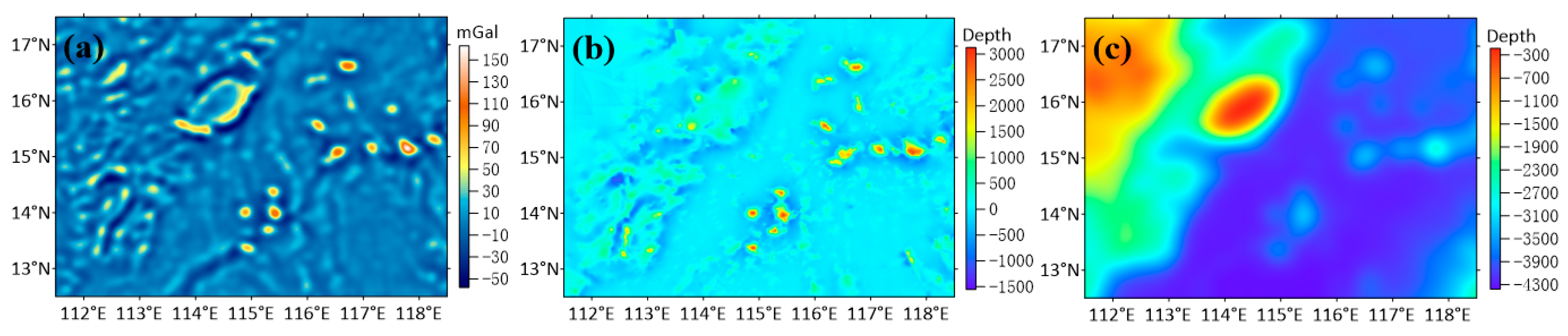
The results of the difference between the crustal density and the seawater density in the study area are influenced by the variation of the seawater depth, and the model of density contrast is more consistent with the variation of the seafloor topography. The relationship between density contrast and seawater depth is an exponential function. In shallow areas, the density difference is large and varies sharply, while in the deep regions, the density difference is relatively small and varies gently. In addition, the results of the frequency domain correlation analysis show that the gravity anomaly in the study area is highly correlated with the seafloor topography in the wavelength range from 25 km to 100 km.
(3)
The accuracy evaluation of the seafloor topography model based on shipboard measured data found that the RMSE of the ST1 estimation using the VDTCCM method is 133.73 m, which is about 5.01% better than the accuracy of ST2 inversion using constant density contrast correction. ST1 is about 23.34% and 39.42% better than the international models ETOPO1 and DTU10, respectively. Moreover, the results of a linear regression fitting between the predicted depth of the four models and the real depth of the SSD show that the discrete dots of the ST1 model are more concentrated and have larger correlation coefficients. Thus, it is shown that the seafloor topography corrected with the VDTCCM method is closer to the external SSD, reflecting the superiority of the method.
(4)
The accuracy of the model is affected by the variation of seawater depth, and the accuracy of the ST1 is significantly better than that of the ST2 in the depth range from 0 to 2000 m. Therefore, it is necessary to consider the density variation of seawater in the middle and shallow areas. From the distribution of the larger error points, the error points of the four models are mainly distributed in the rugged Zhongsha Islands and the areas around the seamounts, while the error points are relatively less distributed in the areas with gentle topographic changes in the Central Basin. Significantly, the ST1 exhibits more topographic details as a result of the power density spectral analysis.

Author Contributions

Y.S. and W.Z. designed the research; Y.S. and Z.L. performed the experiments; Y.S., Z.Z. and X.Z. wrote this paper. All authors have read and agreed to the published version of the manuscript.

Funding

This work was supported in part by the National Natural Science Foundation of China (under grant 42274119), in part by the Liaoning Revitalization Talents Program (under grant XLYC2002082), in part by the National Key Research and Development Plan Key Special Projects of Science and Technology Military Civil Integration (2022YFF1400500), and in part by the Key Project of Science and Technology Commission of the Central Military Commission.

Institutional Review Board Statement

Not applicable.

Informed Consent Statement

Not applicable.

Data Availability Statement

Not applicable.

Acknowledgments

The authors are thankful to the National Geophysical Data Center (https://www.ngdc.noaa.gov/mgg/global/global.html, accessed on 2 September 2022) for providing the depth data of the shipborne measurements and the ETOPO1 bathymetric model, and are thankful to the Scripps Institution of Oceanography website (https://topex.ucsd.edu/marine_grav/mar_grav.html, accessed on 2 September 2022) for providing the V32.1 gravity anomaly and SIO 24.1 seafloor topography. We are grateful the Technical University of Denmark (https://www.space.dtu.dk/english, accessed on 2 September 2022) for the DTU10 bathymetric model. We also hank anonymous reviewers for their suggestions.

Conflicts of Interest

The authors declare no conflict of interest.

References

  1. Sandwell, D.T.; Smith, W.H.F.; Gille, S.; Kappel, E.; Jayne, S.; Soofi, K.; Coakley, B.; Geli, L. Bathymetry from space: Rationale and requirements for a new, high-resolution altimetric mission. Comptes Rendus Geosci. 2006, 338, 1049–1062. [Google Scholar] [CrossRef]
  2. Chen, P.Y.; Li, Y.; Su, Y.M.; Chen, X.L.; Jiang, Y.Q. Review of AUV underwater terrain matching navigation. J. Navig. 2015, 68, 1155–1172. [Google Scholar] [CrossRef]
  3. Zhao, D.N.; Wu, Z.Y.; Zhou, J.Q.; Li, J.B.; Shang, J.H.; Li, S.J. A new method of automatic SVP optimization based on MOV algorithm. Mar. Geod.. 2015, 38, 225–240. [Google Scholar] [CrossRef]
  4. Klemas, V. Beach profiling and Lidar bathymetry: An overview with case studies. J. Coast Res. 2011, 27, 1019–1028. [Google Scholar] [CrossRef]
  5. Muzirafuti, A.; Barreca, G.; Crupi, A.; Faina, G.; Paltrinieri, D.; Lanza, S.; Randazzo, G. The contribution of multispectral satellite image to shallow water bathymetry mapping on the coast of Misano Adriatico, Italy. J. Mar. Sci. Eng. 2020, 8, 126. [Google Scholar] [CrossRef]
  6. Dixon, T.H.; Naraghi, M.; Mcnutt, M.K.; Smith, S.M. Bathymetric prediction from SEASAT altimeter data. J. Geophys. Res. 1983, 88, 1563–1571. [Google Scholar] [CrossRef]
  7. Li, Z.; Guo, J.Y.; Ji, B.; Wan, X.Y.; Zhang, S.J. A Review of Marine Gravity Field Recovery from Satellite Altimetry. Remote Sens. 2022, 14, 4790. [Google Scholar] [CrossRef]
  8. Smith, W.H.F.; Sandwell, D.T. Bathymetric prediction from dense satellite altimetry and sparse shipboard bathymetry. J. Geophys. Res. 1994, 99, 21803–21824. [Google Scholar] [CrossRef]
  9. Parker, R.L. The rapid calculation of potential anomalies. Geophys. J. Int. 1973, 31, 447–455. [Google Scholar] [CrossRef]
  10. Fan, D.; Li, S.S.; Meng, S.Y.; Zhang, J.H.; Shan, J.C.; Wang, A.M. Applying robust estimation method to estimate seafloor topography in the Sea of Japan. J. Chin. Inert. Tech. 2020, 28, 576–585. [Google Scholar]
  11. Ibrahim, A.; Hinze, W.J. Mapping buried bedrock topography with gravity. Ground Water 1972, 10, 18–23. [Google Scholar] [CrossRef]
  12. Kim, J.W.; Frese, R.R.B.; Lee, B.Y.; Roman, D.R.; Doh, S. Altimetry-derived gravity predictions of bathymetry by the Gravity-Geologic Method. Pure Appl. Geophys. 2011, 168, 815–826. [Google Scholar] [CrossRef]
  13. Xiang, X.S.; Wan, X.Y.; Zhang, R.N.; Li, Y.; Sui, X.H.; Wang, W.B. Bathymetry inversion with the gravity-geologic method: A study of long-wavelength gravity modeling based on adaptive mesh. Mar. Geod. 2017, 40, 329–340. [Google Scholar] [CrossRef]
  14. Sun, Y.J.; Zheng, W.; Li, Z.W.; Zhou, Z.Q. Improved the accuracy of seafloor topography from altimetry-derived gravity by the topography constraint factor weight optimization method. Remote Sens. 2021, 13, 2277. [Google Scholar] [CrossRef]
  15. Calmant, S. Seamount topography by least-squares inversion of altimetric geoid heights and shipborne profiles of bathymetry and/or gravity anomalies. Geophys. J. Int. 1994, 119, 428–452. [Google Scholar] [CrossRef]
  16. Jena, B.; Kurian, P.J.; Swain, D.; Tyagi, A.; Ravindra, R. Prediction of bathymetry from satellite altimeter based gravity in the Arabian Sea: Mapping of two unnamed deep seamounts. Int. J. Appl. Earth Obs. Geoinf. 2012, 16, 1–4. [Google Scholar] [CrossRef]
  17. Annan, R.F.; Wan, X.Y. Recovering bathymetry of the Gulf of Guinea using altimetry-derived gravity field products combined via convolutional neural network. Surv. Geophys. 2022, 43, 1541–1561. [Google Scholar] [CrossRef]
  18. Wan, X.Y.; Annan, R.F.; Ziggah, Y.Y. Altimetry-derived gravity gradients using spectral method and their performance in bathymetry inversion using back-progragation neural network. J. Geophys. Res. Solid Earth 2023, 128, e2022JB025785. [Google Scholar] [CrossRef]
  19. Sun, H.Y.; Feng, Y.K.; Fu, Y.G.; Sun, W.K.; Peng, C.; Zhou, X.H.; Zhou, D.X. Bathymetric prediction using multisource gravity data derived from a parallel linked BP neural network. J. Geophys. Res. Solid Earth 2023, 127, e2022JB024428. [Google Scholar] [CrossRef]
  20. Fan, D.; Li, S.S.; Meng, S.Y.; Xing, Z.B.; Zhang, C.; Yang, J.J.; Wan, X.Y.; Qu, Z.H. Applying iterative method to solving high-order terms of seafloor topography. Mar. Geod. 2020, 43, 63–85. [Google Scholar] [CrossRef]
  21. Oldenburg, D.W. The inversion and interpretation of gravity anomalies. Geophysics 1974, 39, 526–536. [Google Scholar] [CrossRef]
  22. Xu, C.; Li, J.B.; Wu, Y.L. Improved gravity-geologic method and its application to seafloor topography inversion in the South China Sea. Geophys. Inf. Sci. Wuhan Univ. 2022. [Google Scholar] [CrossRef]
  23. Yu, J.H.; An, B.; Xu, H.; Sun, Z.M.; Tian, Y.W.; Wang, Q.Y. An iterative algorithm for predicting seafloor topography from gravity anomalies. Remote Sens. 2023, 15, 1069. [Google Scholar] [CrossRef]
  24. Garcia-Adbeslem, J. 2-D inversion of gravity data using sources laterally bounded by continuous surfaces and depth-dependent density. Geophysics 2000, 65, 1128–1141. [Google Scholar] [CrossRef]
  25. Zhang, S.; Zhang, M.H.; Liu, L.; Qiao, J.H.; Liu, S.F. Improved interface inversion based on constrained varying density and its application. Chin. J. Geophys. 2020, 63, 3886–3895. [Google Scholar]
  26. Silva, J.B.C.; Costa, D.C.L.; Barbosa, V.C.F. Gravity inversion of basement relief and estimation of density contrast variation with depth. Geophysics 2006, 71, J51–J58. [Google Scholar] [CrossRef]
  27. Chakravarthi, V.; Kumar, P.M.; Ramama, B.; Sastry, S.R. Automatic gravity modeling of sedimentary basins by means of polygonal source geometry and exponential density contrast variation: Two space domain based algorithms. J. Appl. Geophy. 2016, 124, 54–61. [Google Scholar] [CrossRef]
  28. Brown, W.S. Physical properties of seawater. Springer Handbook of Ocean Engineering; Dhanak, M.R., Xiros, N.I., Eds.; Springer: Berlin/Heidelberg, Germany, 2016; pp. 101–110. [Google Scholar]
  29. Li, H.L.; Wu, Z.C.; Ji, F. Crustal density structure of the northern South China Sea from constrained 3-D gravity inversion. Chin. J. Geophys. 2020, 36, 1894–1912. [Google Scholar]
  30. Wu, L.Y. Efficient modelling of gravity effects due to topographic masses using the Gauss–FFT method. Geophys J. Int. 2016, 205, 160–178. [Google Scholar] [CrossRef]
  31. Marks, K.M.; Smith, W.F. Radially symmetric coherence between satellite gravity and multibeam bathymetry grids. Mar. Geophys. Res. 2012, 33, 223–227. [Google Scholar] [CrossRef]
  32. Wan, X.Y.; Han, W.P.; Ran, J.J.; Ma, W.J.; Annan, R.F.; Li, B. Seafloor density contrast derived from gravity and shipborne depth observations: A case study in a local area of Atlantic Ocean. Front. Earth Sci. 2021, 9, 668863. [Google Scholar] [CrossRef]
  33. Qin, X.W.; Zhao, B.; Li, F.Y.; Zhang, B.J.; Wang, H.J.; Zhang, R.W.; He, J.X.; Chen, X. Deep structural research of the South China Sea: Progress and directions. Geol. China 2019, 2, 530–540. [Google Scholar] [CrossRef]
  34. Amante, C.; Eakins, B.W. ETOPO1 1 Arc-Minute Global Relief Model: Procedures, Data Sources and Analysis; National Geophysical Data Center: Boulder, CO, USA, 2009; pp. 1–25. [Google Scholar]
  35. Sandwell, D.T.; Garcia, E.; Soofi, K.; Wessel, P.; Chandler, M.; Smith, W.H.F. Toward 1-mGal accuracy in global marine gravity from CryoSat-2, Envisat, and Jason-1. Lead. Edge 2013, 32, 892–899. [Google Scholar] [CrossRef]
  36. Andersen, O.B.; Knudsen, P. The DNSC08BAT Bathymetry Developed from Satellite Altimetry; EGU-2008 Meeting: Vienna, Austria, 2008. [Google Scholar]
  37. Laske, G.; Masters, G.; Ma, Z.T.; Pasyanos, M. Update on CRUST1.0—A 1-degree global model of Earth’s crust. In Proceedings of the EGU General Assembly 2013, Vienna, Austria, 7–12 April 2013. [Google Scholar]
  38. Gladkikh, V.; Tenzer, R. A mathematical model of the global ocean saltwater density distribution. Pure Appl. Geophys. 2011, 169, 249–257. [Google Scholar] [CrossRef]
Figure 1. Overview and experimental data of the research area: (a) overview of the study area with the ETOPO1 model in the background and (b) the gravity anomaly derived via satellite altimetry; the black dots in the figure are the control data and the red dots are the check data.
Jmse 11 00853 g001
Figure 2. Results of the density model: (a) density model of crust, (b) density model of seawater, and (c) density contrast model.
Jmse 11 00853 g002
Figure 3. The fitted results of the density contrast: (a) fitted curve of the density contrast with depth and (b) fitted density contrast model.
Jmse 11 00853 g003
Figure 4. Results of the coherency between the gravity anomaly and seafloor topography changing with wavelength.
Jmse 11 00853 g004
Figure 5. Filtering results for the gravity anomaly and seafloor topography: (a) band-pass filtering and downward continuation result for the gravity anomaly, (b) medium and short wavelengths for the seafloor topography, and (c) low-pass filtering result for the SIO seafloor topography.
Jmse 11 00853 g005
Figure 6. Flowchart of the seafloor topography inversion process.
Jmse 11 00853 g006
Figure 7. The model of the seafloor topography generated via (a) ST1, (b) ST, (c) ETOPO1, and (d) DTU10. The magenta boxes indicate the locations of the Xisha Islands, Zhongsha Islands, Zhongsha North Ridge, and Zhongnanhai Mountain.
Jmse 11 00853 g007
Figure 8. Regression fitting results of the predicted depth of four different models and the real depth of the SSD: (a) the result for ST1, (b) the result for ST2, (c) the result for ETOPO1, and (d) the result for DTU10. The red line indicates the fitted result. R2 is the fitted correlation coefficient.
Jmse 11 00853 g008
Figure 9. Accuracy variation curve with depth. The black square line is for the ST1, the red circular line is for the ST2, the blue triangular line is for the ETOPO1 model, and the green star-shaped line is for the DTU10 model.
Jmse 11 00853 g009
Figure 10. Results for the distribution of larger error dots: (a) ST1 (282), (b) ST2 (342), (c) ETOPO1 (462), and (d) DTU10 (316). The numbers indicate the number of error points.
Jmse 11 00853 g010
Figure 11. Analytical results of the topographic power spectra density: (a) variation curve of the power spectral density and (b) curve of the difference in power spectral density.
Jmse 11 00853 g011
Table 1. Statistical results of the experimental data.
DataMaxMinMeanMedianSTD
Control points of SSD−23.00 m−4992.7 m−3802.68 m−4117.00 m708.77 m
Check points of SSD−364.00 m−4436.50 m−3762.05 m−4102.40 m780.62 m
Gravity anomaly207.38 mGal59.50 mGal8.04 mGal6.31 mGal20.49 mGal
Table 2. Statistical results of the difference between the model values and check data. Unit: m.
ModelMaxMinMeanMedianSTDRMSE
ST1-SSD563.94−1124.08−13.70−8.95133.02133.73
ST2-SSD577.75−1212.33−15.66−8.63139.91140.78
ETOPO1-SSD1019.13−1060.51−20.92−16.03173.18174.44
DTU10-SSD2147.95−1996.8258.9969.00212.73220.76
Table 3. Statistical results of the differences between the models and check data in different depth ranges. Unit: m.
RangeModelMaxMinMeanMedianRMSE
>1000
(183 #)
ST1133.55−775.50−285.14−177.25383.07
ST249.96−976.26−549.68−497.15587.22
ETOPO1279.07−680.84−100.25−54.12289.45
DTU10734.86−1996.82−109.72154.77610.56
1000~2000 (734)ST1359.97−1124.08−39.46−0.72178.22
ST2342.50−1212.33−40.091.75187.69
ETOPO1522.91−1060.51−144.10−118.99292.74
DTU101641.39−1503.22−70.54−22.62380.27
2000~3000 (1676)ST1503.17−824.84−30.663.67201.30
ST2528.68−766.83−25.544.28194.72
ETOPO1951.71−868.28−35.09−24.99244.26
DTU102147.95−933.341.847.12299.47
3000~4000
(4181)
ST1546.57−809.83−13.92−3.48181.37
ST2555.18−840.52−13.08−3.34180.82
ETOPO11019.13−837.69−39.82−16.03236.00
DTU101884.64−827.4922.3719.52211.14
>4000 (10241)ST1563.94−355.08−4.13−10.1168.23
ST2577.75−355.84−3.80−10.0168.48
ETOPO1999.51−411.57−0.64−14.72102.03
DTU10694.64−348.0795.5896.02175.67
# The data in parentheses indicate the number of check data points in this depth range.
Disclaimer/Publisher’s Note: The statements, opinions and data contained in all publications are solely those of the individual author(s) and contributor(s) and not of MDPI and/or the editor(s). MDPI and/or the editor(s) disclaim responsibility for any injury to people or property resulting from any ideas, methods, instructions or products referred to in the content.

