
Particulate Matter (PM1, 2.5, 10) Concentration Prediction in Ship Exhaust Gas Plume through an Artificial Neural Network


Abstract
:1. Introduction
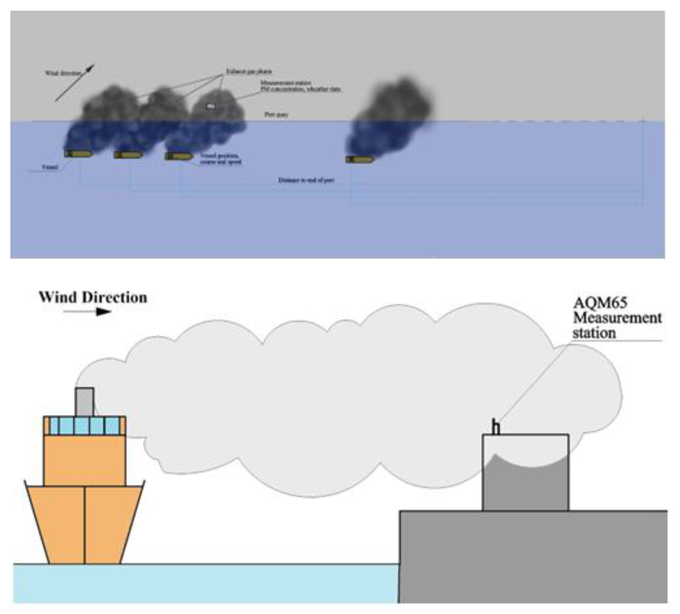
2. Materials and Methods
2.1. Ship Technical-Specification Data
2.2. Weather Data
2.3. AIS Data
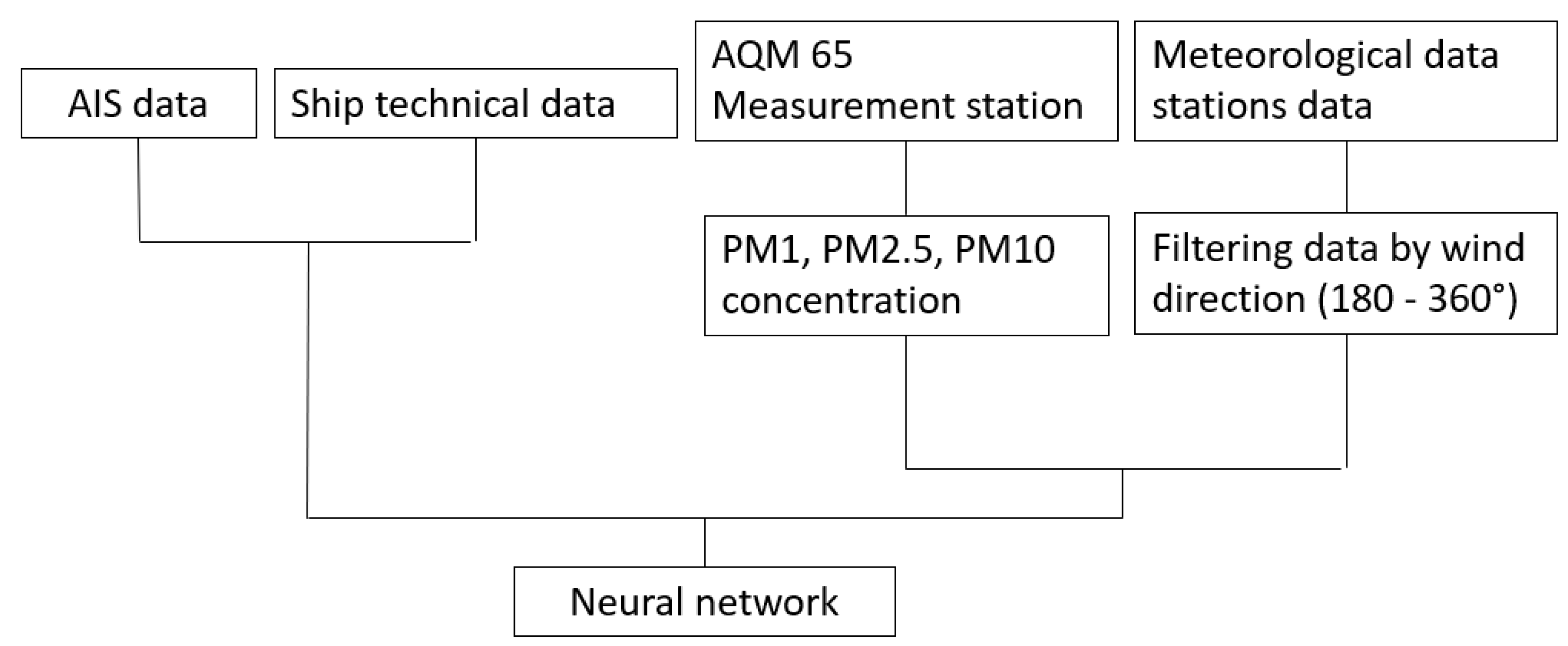
2.4. Neural Network
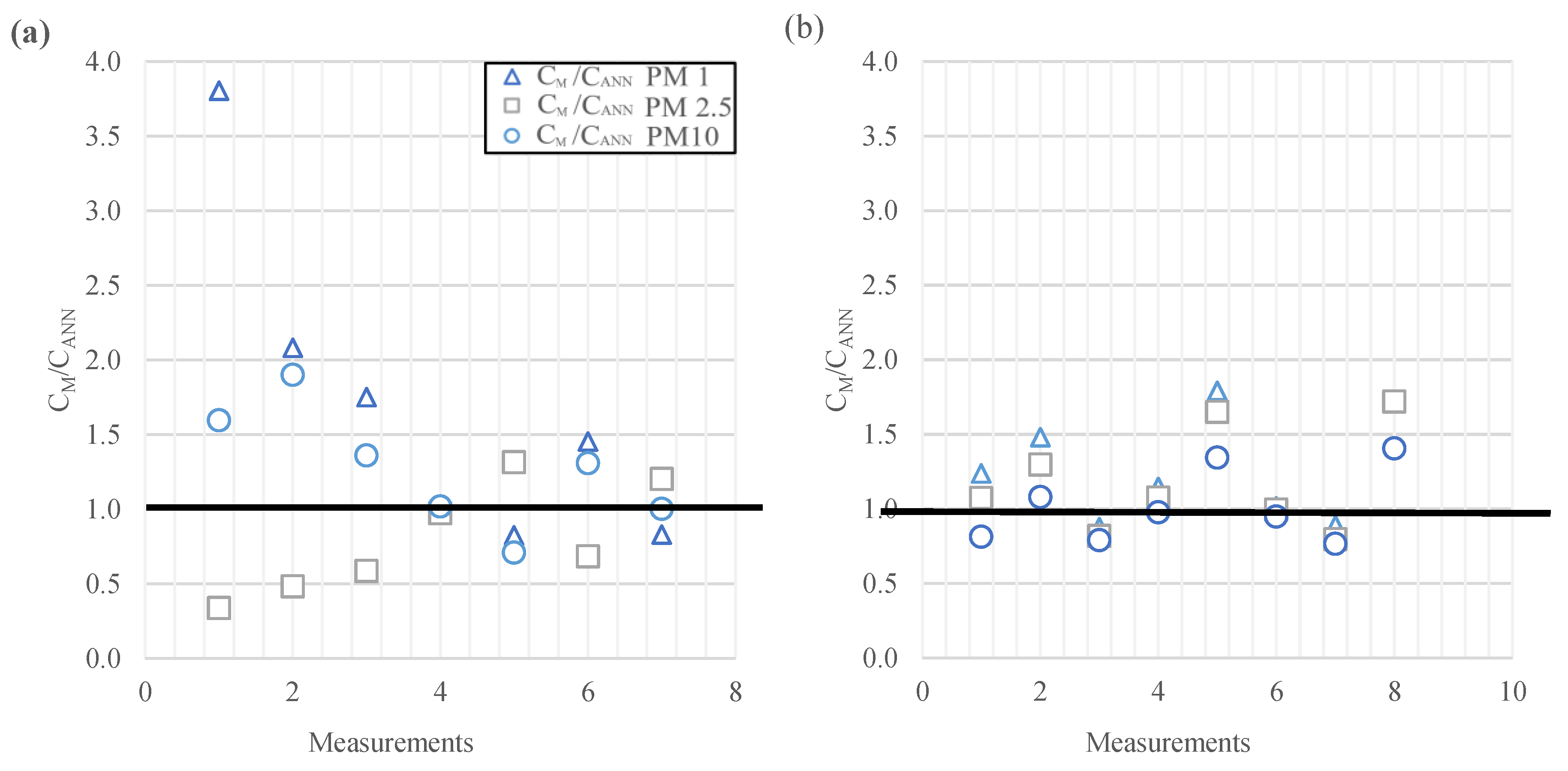
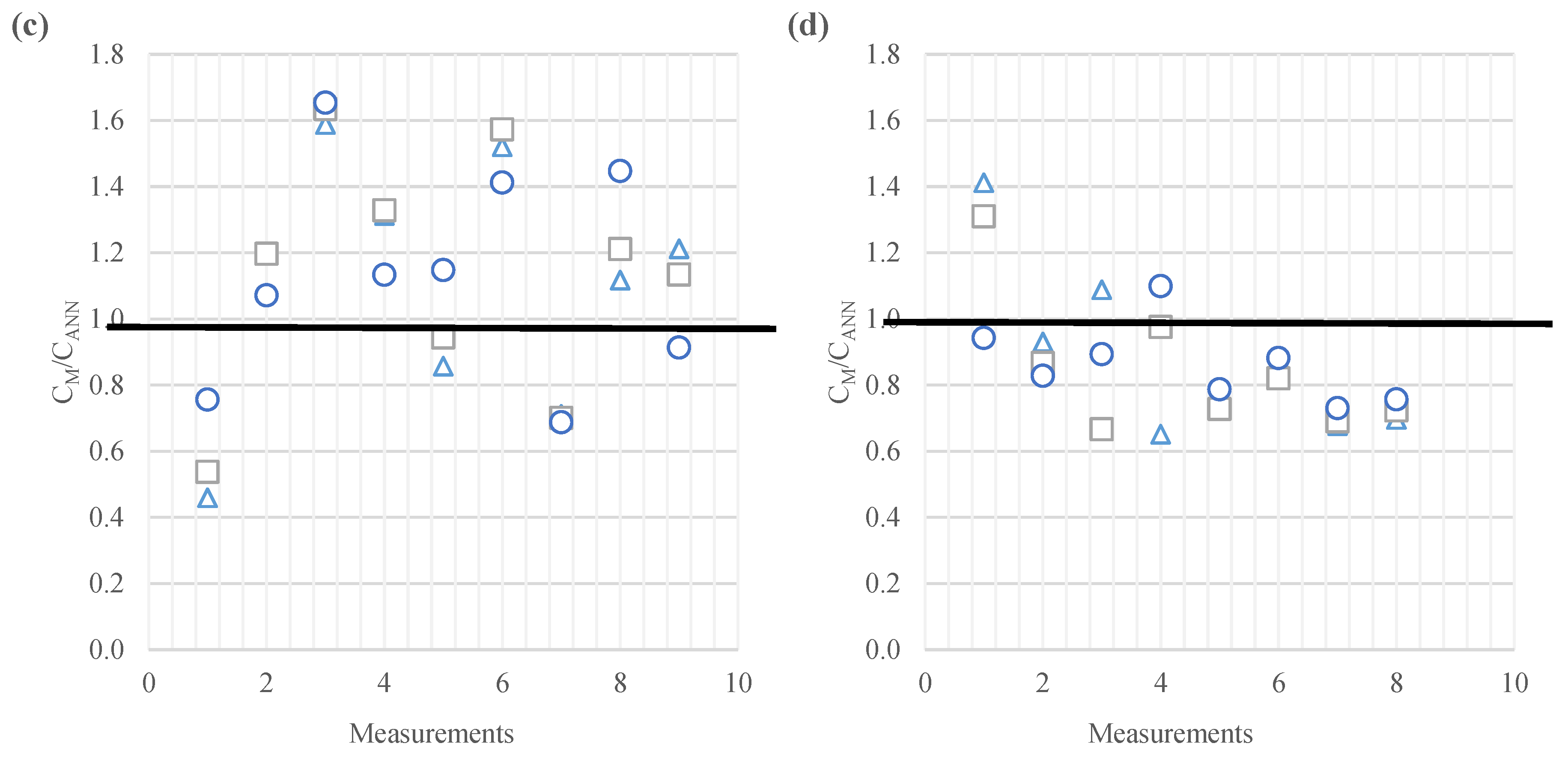
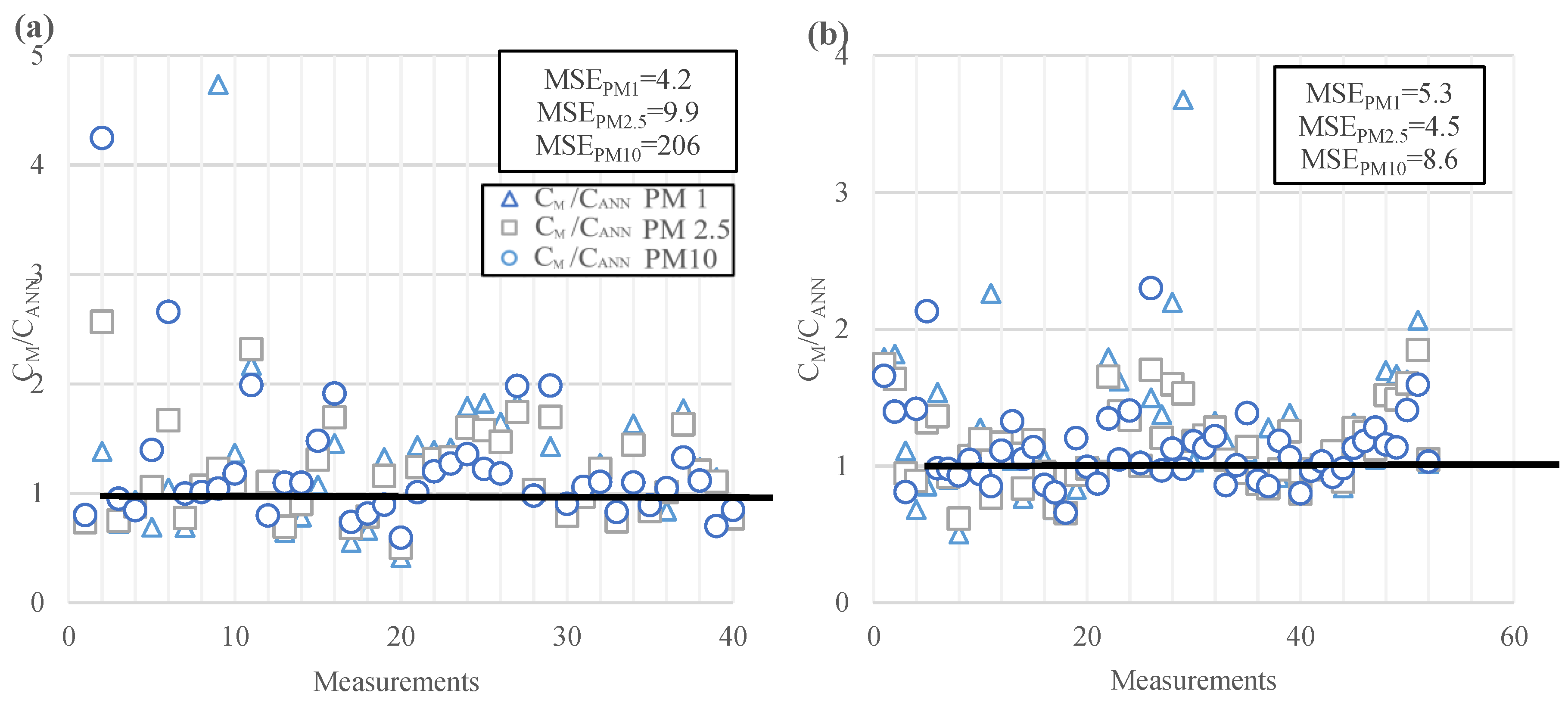
3. Results and Discussions
4. Conclusions
Author Contributions
Funding
Institutional Review Board Statement
Informed Consent Statement
Data Availability Statement
Conflicts of Interest
Nomenclature
| AIS | automatic identification system |
| ANN | artificial neural network |
| CANN | concentration calculated by the trained ANN |
| CM | measured pollutant concentration |
| CO2 | carbon dioxide |
| DWT | deadweight tonnage |
| EU | European union |
| GT | gross tonnage |
| IMO | international maritime organization |
| NOx | nitrogen oxides |
| PM | particulate matter |
| SOx | sulfur oxides |
| TSP | total suspended particles |
References
- European Commission. Amended Proposal for a Regulation of the European Parliament and of the Council on Establishing the Framework for Achieving Climate Neutrality and Amending Regulation (EU) 2018/1999 (European Climate Law); COM(2020) 563 Final; European Commission: Brussels, Belgium, 2020. [Google Scholar]
- European Commission. Communication from the Commission to the European Parliament, the Council, the European Economic and Social Committee and the Committee of the Regions Stepping Up Europe’s 2030 Climate Ambition Investing in a Climate-Neutral Future for the Benefit of Our People; COM(2020) 562 Final; European Commission: Brussels, Belgium, 2020. [Google Scholar]
- European Commission. Commission Staff Working Document Full-Length Report Accompanying the Document Report from the Commission 2019 Annual Report on CO2 Emissions from Maritime Transport; SWD(2020) 82 Final; European Commission: Brussels, Belgium, 2020. [Google Scholar]
- European Commission. Proposal for a Regulation of the European Parliament and of the Council on the Use of Renewable and Low-Carbon Fuels in Maritime Transport and Amending Directive 2009/16/EC; COM(2021) 562 Final; European Commission: Brussels, Belgium, 2021. [Google Scholar]
- European Environment Agency. Aviation and Shipping: Impacts on Europe’s Environment: TERM 2017: Transport and Environment Reporting Mechanism (TERM) Report; Publications Office: Luxembourg, 2018.
- European Environment Agency. The Impact of International Shipping on European Air Quality and Climate Forcing; Publications Office: Luxembourg, 2013.
- United Nations Conference on Trade and Development. Review of Maritime Transport 2021; United Nations: Geneva, Switzerland, 2021; ISBN 978-92-1-113026-3. [Google Scholar]
- Gavalas, D.; Syriopoulos, T.; Tsatsaronis, M. COVID–19 impact on the shipping industry: An event study approach. Transp. Policy 2021, 116, 157–164. [Google Scholar] [CrossRef] [PubMed]
- European Maritime Safety Agency. COVID-19—Impact on Shipping; EMSA: Lisbon, Portugal, 2022; p. 23.
- Millefiori, L.M.; Braca, P.; Zissis, D.; Spiliopoulos, G.; Marano, S.; Willett, P.K.; Carniel, S. COVID-19 impact on global maritime mobility. Sci. Rep. 2021, 11, 18039. [Google Scholar] [CrossRef] [PubMed]
- Mamoudou, I.; Zhang, F.; Chen, Q.; Wang, P.; Chen, Y. Characteristics of PM2.5 from ship emissions and their impacts on the ambient air: A case study in Yangshan Harbor, Shanghai. Sci. Total Environ. 2018, 640–641, 207–216. [Google Scholar] [CrossRef] [PubMed]
- Kim, Y.; Moon, N.; Chung, Y.; Seo, J. Impact of IMO Sulfur Regulations on Air Quality in Busan, Republic of Korea. Atmosphere 2022, 13, 1631. [Google Scholar] [CrossRef]
- Mao, J.; Zhang, Y.; Yu, F.; Chen, J.; Sun, J.; Wang, S.; Zou, Z.; Zhou, J.; Yu, Q.; Ma, W.; et al. Simulating the impacts of ship emissions on coastal air quality: Importance of a high-resolution emission inventory relative to cruise- and land-based observations. Sci. Total Environ. 2020, 728, 138454. [Google Scholar] [CrossRef]
- Toscano, D.; Murena, F. Atmospheric ship emissions in ports: A review. Correlation with data of ship traffic. Atmospheric Environ. X 2019, 4, 100050. [Google Scholar] [CrossRef]
- Toscano, D.; Murena, F.; Quaranta, F.; Mocerino, L. Assessment of the impact of ship emissions on air quality based on a complete annual emission inventory using AIS data for the port of Naples. Ocean Eng. 2021, 232, 109166. [Google Scholar] [CrossRef]
- World Health Organization (WHO). Health Risks of Air Pollution in Europe—HRAPIE Project, Recommendations for Concentration–Response Functions for Cost–Benefit Analysis of Particulate Matter, Ozone and Nitrogen Dioxide; WHO Regional Office for Europe: Copenhagen, Denmark, 2013; p. 60. [Google Scholar]
- Firląg, S.; Rogulski, M.; Badyda, A. The Influence of Marine Traffic on Particulate Matter (PM) Levels in the Region of Danish Straits, North and Baltic Seas. Sustainability 2018, 10, 4231. [Google Scholar] [CrossRef] [Green Version]
- Gregório, J.; Gouveia-Caridade, C.; Caridade, P.J.S.B. Modeling PM2.5 and PM10 Using a Robust Simplified Linear Regression Machine Learning Algorithm. Atmosphere 2022, 13, 1334. [Google Scholar] [CrossRef]
- Šilas, G.; Rapalis, P. Review of Methods and Models for Estimating Ship Emissions in Port. In Transport Means 2021, Proceedings of the 25th International Scientific Conference, Kaunas, Lithuania, 6–8 October 2021; Technologija: Kaunas, Lithuania, 2021; pp. 955–960. [Google Scholar]
- Anand, A.; Wei, P.; Gali, N.K.; Sun, L.; Yang, F.; Westerdahl, D.; Zhang, Q.; Deng, Z.; Wang, Y.; Liu, D.; et al. Protocol development for real-time ship fuel sulfur content determination using drone based plume sniffing microsensor system. Sci. Total Environ. 2020, 744, 140885. [Google Scholar] [CrossRef]
- Shen, L.; Wang, Y.; Liu, K.; Yang, Z.; Shi, X.; Yang, X.; Jing, K. Synergistic path planning of multi-UAVs for air pollution detection of ships in ports. Transp. Res. Part E: Logist. Transp. Rev. 2020, 144, 102128. [Google Scholar] [CrossRef]
- Wang, X.; Shen, Y.; Lin, Y.; Pan, J.; Zhang, Y.; Louie, P.K.K.; Li, M.; Fu, Q. Atmospheric pollution from ships and its impact on local air quality at a port site in Shanghai. Atmos. Chem. Phys. 2019, 19, 6315–6330. [Google Scholar] [CrossRef] [Green Version]
- Goldsworthy, L.; Goldsworthy, B. Modelling of ship engine exhaust emissions in ports and extensive coastal waters based on terrestrial AIS data—An Australian case study. Environ. Model. Softw. 2015, 63, 45–60. [Google Scholar] [CrossRef]
- Tichavska, M.; Tovar, B.; Gritsenko, D.; Johansson, L.; Jalkanen, J.P. Air emissions from ships in port: Does regulation make a difference? Transp. Policy 2019, 75, 128–140. [Google Scholar] [CrossRef]
- Zou, Z.; Zhao, J.; Zhang, C.; Zhang, Y.; Yang, X.; Chen, J.; Xu, J.; Xue, R.; Zhou, B. Effects of cleaner ship fuels on air quality and implications for future policy: A case study of Chongming Ecological Island in China. J. Clean. Prod. 2020, 267, 122088. [Google Scholar] [CrossRef]
- Topic, T.; Murphy, A.J.; Pazouki, K.; Norman, R. Assessment of ship emissions in coastal waters using spatial projections of ship tracks, ship voyage and engine specification data. Clean. Eng. Technol. 2021, 2, 100089. [Google Scholar] [CrossRef]
- Ding, W.; Zhu, Y. Prediction of PM2.5 Concentration in Ningxia Hui Autonomous Region Based on PCA-Attention-LSTM. Atmosphere 2022, 13, 1444. [Google Scholar] [CrossRef]
- Hong, H.; Choi, I.; Jeon, H.; Kim, Y.; Lee, J.-B.; Park, C.H.; Kim, H.S. An Air Pollutants Prediction Method Integrating Numerical Models and Artificial Intelligence Models Targeting the Area around Busan Port in Korea. Atmosphere 2022, 13, 1462. [Google Scholar] [CrossRef]
- Qiao, Z.; Cui, S.; Pei, C.; Ye, Z.; Wu, X.; Lei, L.; Luo, T.; Zhang, Z.; Li, X.; Zhu, W. Regional Predictions of Air Pollution in Guangzhou: Preliminary Results and Multi-Model Cross-Validations. Atmosphere 2022, 13, 1527. [Google Scholar] [CrossRef]
- Li, D.; Liu, J.; Zhao, Y. Prediction of Multi-Site PM2.5 Concentrations in Beijing Using CNN-Bi LSTM with CBAM. Atmosphere 2022, 13, 1719. [Google Scholar] [CrossRef]
- Jiang, H.; Wang, X.; Sun, C. Predicting PM2.5 in the Northeast China Heavy Industrial Zone: A Semi-Supervised Learning with Spatiotemporal Features. Atmosphere 2022, 13, 1744. [Google Scholar] [CrossRef]
- Kujawska, J.; Kulisz, M.; Oleszczuk, P.; Cel, W. Machine Learning Methods to Forecast the Concentration of PM10 in Lublin, Poland. Energies 2022, 15, 6428. [Google Scholar] [CrossRef]
- Li, D.; Liu, J.; Zhao, Y. Forecasting of PM2.5 Concentration in Beijing Using Hybrid Deep Learning Framework Based on Attention Mechanism. Appl. Sci. 2022, 12, 11155. [Google Scholar] [CrossRef]
- Galvão, S.L.J.; Matos, J.C.O.; Kitagawa, Y.K.L.; Conterato, F.S.; Moreira, D.M.; Kumar, P.; Nascimento, E.G.S. Particulate Matter Forecasting Using Different Deep Neural Network Topologies and Wavelets for Feature Augmentation. Atmosphere 2022, 13, 1451. [Google Scholar] [CrossRef]
- Peralta, B.; Sepúlveda, T.; Nicolis, O.; Caro, L. Space-Time Prediction of PM2.5 Concentrations in Santiago de Chile Using LSTM Networks. Appl. Sci. 2022, 12, 11317. [Google Scholar] [CrossRef]
- Ko, K.-K.; Jung, E.-S. Improving Air Pollution Prediction System through Multimodal Deep Learning Model Optimization. Appl. Sci. 2022, 12, 10405. [Google Scholar] [CrossRef]
- Yan, R.; Liao, J.; Yang, J.; Sun, W.; Nong, M.; Li, F. Multi-hour and multi-site air quality index forecasting in Beijing using CNN, LSTM, CNN-LSTM, and spatiotemporal clustering. Expert Syst. Appl. 2021, 169, 114513. [Google Scholar] [CrossRef]
- Schaub, M.; Baldauf, M.; Hassel, E. Prediction of PM Emissions during Transient Operation of Marine Diesel Engines Using Artificial Neural Networks; ARGESIM Publisher: Vienna, Austria, 2020; pp. 167–174. [Google Scholar]
- Lin, S.; Zhao, J.; Li, J.; Liu, X.; Zhang, Y.; Wang, S.; Mei, Q.; Chen, Z.; Gao, Y. A Spatial–Temporal Causal Convolution Network Framework for Accurate and Fine-Grained PM2.5 Concentration Prediction. Entropy 2022, 24, 1125. [Google Scholar] [CrossRef]
- Aeroqual. AQM 65. Available online: https://www.aeroqual.com/products/aqm-stations/aqm-65-air-quality-monitoring-station#specifications (accessed on 27 November 2022).
- Freemeteo. Orai Klaipėda—Ankstesnė Orų Informacija, Pateikiama Kiekvieną Dieną. Available online: https://freemeteo.lt/orai/klaipeda/istorija/kiekvienos-dienos-ankstesni-duomenys/?gid=598098&station=6334&date=2022-11-27&language=lithuanian&country=lithuania (accessed on 27 November 2022).
- Neural Designer. Explainable AI Platform. Available online: https://www.neuraldesigner.com/ (accessed on 10 June 2022).
- Wang, K.; Wang, J.; Huang, L.; Yuan, Y.; Wu, G.; Xing, H.; Wang, Z.; Wang, Z.; Jiang, X. A comprehensive review on the prediction of ship energy consumption and pollution gas emissions. Ocean Eng. 2022, 266, 112826. [Google Scholar] [CrossRef]
- Rapalis, P.; Lebedevas, S.; Mickevičienė, R. Mathematical Modelling of Diesel Engine Operational Performance Parameters in Transient Modes. Pomorstvo 2018, 32, 165–172. [Google Scholar] [CrossRef]
- Barberi, S.; Sambito, M.; Neduzha, L.; Severino, A. Pollutant Emissions in Ports: A Comprehensive Review. Infrastructures 2021, 6, 114. [Google Scholar] [CrossRef]
- Sui, C.; de Vos, P.; Stapersma, D.; Visser, K.; Hopman, H.; Ding, Y. Mean value first principle engine model for predicting dynamic behaviour of two-stroke marine diesel engine in various ship propulsion operations. Int. J. Nav. Arch. Ocean Eng. 2022, 14, 100432. [Google Scholar] [CrossRef]
- Hong, H.; Jeon, H.; Youn, C.; Kim, H. Incorporation of Shipping Activity Data in Recurrent Neural Networks and Long Short-Term Memory Models to Improve Air Quality Predictions around Busan Port. Atmosphere 2021, 12, 1172. [Google Scholar] [CrossRef]
- Lee, J.-B.; Roh, M.-I.; Kim, K.-S. Prediction of ship power based on variation in deep feed-forward neural network. Int. J. Nav. Arch. Ocean Eng. 2021, 13, 641–649. [Google Scholar] [CrossRef]
- Lebedevas, S.; Lazareva, N.; Rapalis, P.; Daukšys, V.; Čepaitis, T. Influence of marine fuel properties on ignition, injection delay and energy efficiency. Transport 2021, 36, 339–353. [Google Scholar] [CrossRef]


| Parameter | Dimension |
|---|---|
| DWT | km/h |
| GT | t |
| Ship length | m |
| Beam | m |
| Ship depth | m |
| The total power of the engines | kW |
| Ship draft | m |
| Parameter | Dimension |
|---|---|
| Wind speed | km/h |
| Wind direction | ° |
| Pressure | mb |
| Relative humidity | % |
| Parameter | Dimension |
|---|---|
| Ship speed | km/h |
| Course over ground | ° |
| True heading | ° |
| Longitude | ° |
| Latitude | ° |
| Distance to the end of the port | m |
| Name | Neurons | Activation Function |
|---|---|---|
| Perseptron layer 1 | 17 | Hyperbolic tangent (tahn) |
| Perseptron layer 2 | 150 | Hyperbolic tangent (tahn) |
| Perseptron layer 3 | 80 | Hyperbolic tangent (tahn) |
| Perseptron layer 4 | 4 | Hyperbolic tangent (tahn) |
| Perseptron layer 5 | 4 | Linear |
| Bounding layer | Data range |
Disclaimer/Publisher’s Note: The statements, opinions and data contained in all publications are solely those of the individual author(s) and contributor(s) and not of MDPI and/or the editor(s). MDPI and/or the editor(s) disclaim responsibility for any injury to people or property resulting from any ideas, methods, instructions or products referred to in the content. |
© 2023 by the authors. Licensee MDPI, Basel, Switzerland. This article is an open access article distributed under the terms and conditions of the Creative Commons Attribution (CC BY) license (https://creativecommons.org/licenses/by/4.0/).
Share and Cite
Šilas, G.; Rapalis, P.; Lebedevas, S. Particulate Matter (PM1, 2.5, 10) Concentration Prediction in Ship Exhaust Gas Plume through an Artificial Neural Network. J. Mar. Sci. Eng. 2023, 11, 150. https://doi.org/10.3390/jmse11010150
Šilas G, Rapalis P, Lebedevas S. Particulate Matter (PM1, 2.5, 10) Concentration Prediction in Ship Exhaust Gas Plume through an Artificial Neural Network. Journal of Marine Science and Engineering. 2023; 11(1):150. https://doi.org/10.3390/jmse11010150
Chicago/Turabian StyleŠilas, Giedrius, Paulius Rapalis, and Sergejus Lebedevas. 2023. "Particulate Matter (PM1, 2.5, 10) Concentration Prediction in Ship Exhaust Gas Plume through an Artificial Neural Network" Journal of Marine Science and Engineering 11, no. 1: 150. https://doi.org/10.3390/jmse11010150