Validation and Comparisons of Methodologies Implemented in a RANS-VoF Numerical Model for Applications to Coastal Structures

Abstract

Methodologies to be used in numerical models based on Reynolds-averaged Navier–Stokes (RANS) equations and the volume of fluid (VoF) to deal with waves over coastal structures, which involve wave breaking and overtopping and porous structures, are shown in this manuscript. Two turbulence models, k-ε NLS (non-linear Reynolds stress tensor) and k-ε SCM (stabilized closure model), that are used to avoid the growth of the eddy viscosity, are implemented in the FLUENT^® numerical model. Additionally, equations of momentum and turbulence models are adapted to simulate porous media of coastal structures. Comparisons of performance of k-ε NLS, k-ε SCM and standards k-ε and k-ω SST models in several classical cases of regular and random waves on coastal structures are carried out. It was noticed that the standard k-ε turbulence model, and k-ω SST with less intensity, over-predicted eddy viscosity, caused the decay of the free surface elevation and under-estimated wave overtopping discharge. k-ε NLS and k-ε SCM turbulence models have similar performance, with slightly better results of k-ε NLS, showing good agreement with experimental ones.

1. Introduction

In the last decades, several researchers have investigated wave–structure interactions by means of numerical simulations. However, this task still imposes many difficulties due to complex phenomena which this type of case involves, such as wave reflection, wave breaking, wave run-up/down, wave–porous structure interaction and wave overtopping. Each physical process requires the different abilities of numerical models. Recently, models based on Reynolds-averaged Navier–Stokes (RANS) equations have been developed, validated and applied to this type of problem; however, they still show some issues in correctly predicting all phenomena.

Wave breaking requires an adequate turbulence closure model and the free surface tracking method. Sakai et al. [1] carried out the earliest studies involving wave breaking by using the marked-and-cell (MAC) method, developed by Harlow and Welch [2]. Later, Lemos [3] applied the volume of fluid (VoF) method, originally developed by Hirt and Nichols [4]. Lin and Liu [5] developed a RANS model by using an algebraic Reynolds stress k-ε model in combination with the VoF method, which was validated to spilling breaking waves on a sloping beach, based on experiments of Ting and Kirby [6]. The authors observed that turbulence levels near the breaking point were significantly overestimated compared with the experimental data. Bradford [7] employed the RANS-based Flow-3D model and different turbulence models to simulate the spilling and plunging breakers of Ting and Kirby [6] experiments. The author noticed that turbulent kinetic energy in the wave crest prior to breaking is overpredicted using a k-ε model, resulting in an underprediction of the breaking wave height, and suggested the use of k-ω model. Mayer and Madsen [8] modified the k-ω model, using the vorticity of the mean flow instead of the local mean velocity gradient to estimate the production of turbulent kinetic energy. Thus, the generation of the turbulent kinetic energy was overcome in the potential flow region (wave propagation zone outside the surf zone) and the wave damping over the length of the flume was avoided. Jacobsen et al. [9] implemented in the OpenFOAM model a two-phase flow solver and validated this technique in breaking waves by using the modified k-ω turbulence model proposed by Mayer and Madsen [8]. The authors showed the importance of the mesh aspect ratio on numerical results. Brown et al. [10] used different turbulence models in OpenFOAM to simulate both spilling and plunging breakers and observed the necessity of including the density explicitly in the turbulence transport equations. In addition, they concluded that the overall best model is the nonlinear k-ε model; however, the k-ω model showed improvements in relation to the solution without the turbulence model. Devolver et al. [11] used the OpenFOAM model by using both k-ω and k-ω SST turbulence models to analyze the performance of a buoyancy-modified turbulence model in wave breaking in a numerical wave flume. The authors concluded that buoyance-modified turbulence models significantly reduce the common overestimation of the turbulent kinetic energy in the flow field. Chella et al. [12,13] used the level set method and the k-ω model by means of the REEF3D model, in which a turbulence damping scheme was applied to avoid unphysical turbulence production at the interface between water and air. The authors noticed an underprediction of the turbulent kinetic energy levels in the surf zone. Larsen and Fuhrman [14] developed a formulation of the k-ω turbulence model closure to stabilize the model in nearly potential flow regions and overcome the overestimate turbulence levels in pre- and post-breaking. The authors extended the stabilized closure model formulation to other turbulence models.

The wave overtopping on coastal structures involves simultaneously wave run-up/down and wave breaking. It depends on the structure topology, geometry, material characteristics, incident wave conditions and foreshore bathymetry [15]. Numerical models must be able to simulate these complex physical processes that include turbulence, eddy vortices and strong wave–structure interactions [16]. Soliman et al. [17] investigated regular and random wave overtopping over coastal impermeable structures by using the model developed by Lin and Liu [5], which is based on RANS equations, and employing the k-ε turbulence and nonlinear Reynolds stress models, as well as the VoF method. The authors concluded that empirical equations of overtopping, used for design purposes, underestimate the amount of wave overtopping due to random waves. Tuan and Thin [18] compared both non-linear shallow water (developed by Tuan and Oumeraci [19]) and RANS models (COBRAS-UC [15]) in regular and random wave overtopping on impermeable sea dikes with low vertical crown-walls. The authors concluded that the non-linear shallow water model is efficient and reliable to estimate wave overtopping discharges at sea dikes with relatively low walls. However, the RANS-VoF model has more accuracy in high walls. Recently, de Finis et al. [20] applied the IH2VOF model to investigate the impact of waves on a storm wall for a dike-promenade structure. Several tests were carried out to study the dependence of the wave forces with the wave characteristics and structural dimensions, and a new empirical design formula was proposed.

Many coastal porous structures are applied to protect coastal infrastructures and natural beaches, including submerged breakwaters that protect coasts with minimal degradation (sometimes enrichment) of the marine environment [21]. The wave–porous structure interaction has been investigated by several researchers to understand the flow motion inside and outside of the permeable structure. The study of the action of waves on rock (rubble) mound breakwaters is difficult, because the flow within interstices of blocks, with very complex geometry, is strongly non-stationary and involves moment advection, free boundary and turbulence and air–water interaction [22]. In addition, the small scales of the porous medium require a prohibitive spatial and time discretization of numerical models. To circumvent these difficulties, van Gent [23], Lin and Liu [5], Liu et al. [24], Nakayama and Kuwahara [25], Getachew et al. [26] and Pedras and de Lemos [27], proposed different strategies to develop momentum equations extended by Darcy and Forchheimer terms to consider the drag caused by the porous structure. Van Gent [23] developed a 1DH model based on the non-linear shallow water equations and a two vertical dimensional (2DV) model based on RANS equations to simulate the wave interaction with permeable and impermeable coastal structures. Hur [28] and Hur et al. [29] developed and applied this methodology of adding drag and inertia terms in the Navier–Stokes equations to simulate flows in porous media to 2D/3D cases.

Nowadays, the most used method applied in porous structures is the volume averaging method, in which Navier–Stokes based models are applied to volumes whose scales are larger than scales of porous structures that compose the porous media [30,31]. These models accurately represent nonlinearities, frequency dispersion and wave breaking, overcoming restrictions of simplified models. Hsu et al. [32] developed a model based on the volume-averaged Reynolds-averaged Navier–Stokes (VARANS) equations, in which the turbulence models are extended by additional terms that describe the porosity effect. Garcia et al. [33] applied this methodology to low-crested breakwaters and Lara et al. [34] analyzed cases considering random waves. Losada et al. [15] investigated the interaction of regular and random waves with a rubble mound breakwater by using the COBRAS-UC numerical model. The authors observed problems with computational efficiency, due to the mesh resolution and number of waves to be simulated. In addition, they noticed difficulties in setting empirical drag coefficients of linear and non-linear terms. Del Jesus et al. [35] reformulated VARANS equations developed by Hsu et al. [32] and developed the IH-3VOF model to simulate two-phase flows within porous media. Jensen et al. [36] revised and re-implemented VARANS equations in the OpenFOAM code. Higuera et al. [37] also implemented in this code a hybrid methodology (2D-3D) to optimize the simulation time needed to assess the three-dimensional effect wave interaction with coastal structures. Vanneste and Troch [38] validated the FLOW-3D numerical model, based on RANS equations with additional drag force term in the momentum equations [29] and the VoF method in large physical model tests on a multi-layered breakwater section.

This study aims to compare the performance of methodologies applied to wave–coastal structure interaction problems implemented in a RANS-VoF numerical model. The FLUENT^® numerical model is used for this purpose, in which some methods have already been implemented by the authors to simulate wave propagation and wave interaction with coastal structures, such as wave generation, wave active absorption technique [39,40,41] and random wave generation by JONSWAP/TMA spectrum [41], among others. Additionally, two new major implementations are carried out in this study: the extended Darcy–Forchheimer formulation, which is used to deal with transient flows in porous medium [23]; and closure turbulence models to avoid the growth of turbulent kinetic energy and eddy viscosity and enable nearly constant wave propagation for longtime simulation in a long wave flume, using the relatively recent k-ε closure turbulence model, proposed by Larsen and Fuhrman [14], and the k-ε non-linear Reynolds stress tensor, which was developed and used by Shih et al. [42] and Lin and Liu [5]. Both implementations are fundamental in dealing with simulations of waves over impermeable and porous structures that involve wave breaking, wave run-up/down and wave overtopping. Results obtained with these two turbulence models are compared to those obtained with standard k-ε and k-ω SST turbulence models for several configurations of interaction between waves and structures.

2. Methodology

In this section, equations and methodologies of the FLUENT^® model [43] used in the study cases are shown, including momentum equations, turbulence model equations, porous medium flow equations and numerical conditions. Some are implemented in the original code by means of user-defined functions (UDF).

2.1. Standard Governing Equations of the FLUENT Model

The RANS FLUENT^® model employs the finite volume method to discretize the continuity and momentum equations, which, considering 2D and incompressible flows, are given by [44,45]:

$$\frac{\partial u_i}{\partial x_i}=0$$

(1)

$$\frac{\partial }{\partial t}\left(\rho u_i\right)+u_j\frac{\partial }{\partial x_j}\left(\rho u_i\right)=-\frac{\partial p}{\partial x_i}+\rho g_i+\frac{\partial {\tau }_{ij}}{\partial x_j}-\frac{\partial \rho \left(\overline{u_i^{\prime }{u}_j^{\prime }}\right)}{\partial x_j}+S_{Mi}$$

(2)

$${\tau }_{ij}=\mu \left(\frac{\partial u_i}{\partial x_j}+\frac{\partial u_j}{\partial x_i}\right)$$

(3)

where i, j = 1, 2, ρ is the specific mass, g_i are components of gravity acceleration, u_i are components of velocity, p is the pressure, μ is the dynamics viscosity, τ_ij is the viscous stress tensor, S_Mi is the source term and $-\rho \left(\overline{u_i^{\prime }{u}_j^{\prime }}\right)$ is the Reynolds stress tensor, which, considering the Boussinesq hypothesis proposed in 1877, is as follows:

$$-\rho \left(\overline{u_i^{\prime }{u}_j^{\prime }}\right)=-\frac{2}{3}\rho k{\delta }_{ij}+{\mu }_t\left(\frac{\partial u_i}{\partial x_j}+\frac{\partial u_j}{\partial x_i}\right)$$

(4)

where μ_t is the turbulent viscosity and k is the kinetic energy of turbulence per mass.

Free surface flow motion is defined by the VoF method [4], which is based on the transport equation of the volume fraction, given by:

$$\frac{\partial f}{\partial t}+u_j\frac{\partial f}{\partial x_j}=0$$

(5)

where the volume fraction, f, is a scalar that takes values 0 in the air, 1 in the water and 0.5 in the position of the free surface.

2.2. Turbulence Models

The turbulence equations are used as a closure for the RANS equations. In this study, two standard turbulence models, k-ε and k-ω SST, available in the FLUENT^® model, are employed. Equations of turbulence kinetic energy (k) and dissipation rate (ε) of the standard k-ε model are given by Harlow and Nakayama [46]:

$$\begin{gathered} \frac{\partial }{\partial t}\left(\rho k\right)+\frac{\partial }{\partial x_j}\left(\rho k{u}_j\right)={\mu }_t\left(2S_{ij}{S}_{ij}\right)-\rho \epsilon \\ +\frac{\partial }{\partial x_j}\left[\left(\mu +\frac{{\mu }_t}{{\sigma }_k}\right)\frac{\partial k}{\partial x_j}\right]+S_k \end{gathered}$$

(6)

$$\begin{gathered} \frac{\partial }{\partial t}\left(\rho \epsilon \right)+\frac{\partial }{\partial x_j}\left(\rho \epsilon u_j\right)=C_{1\epsilon }\frac{\epsilon }{k}{\mu }_t\left(2S_{ij}{S}_{ij}\right)-C_{2\epsilon }\rho \frac{{\epsilon }^2}{k} \\ +\frac{\partial }{\partial x_j}\left[\left(\mu +\frac{{\mu }_t}{{\sigma }_{\epsilon }}\right)\frac{\partial \epsilon }{\partial x_j}\right]+S_{\epsilon } \end{gathered}$$

(7)

$${\mu }_t=\rho C_{\mu }\frac{k^2}{\epsilon }$$

(8)

where

$$S_{ij}=\frac{1}{2}\left[\frac{\partial u_j}{\partial x_j}+\frac{\partial u_j}{\partial x_i}\right]$$

(9)

and σ_κ = 1.0, σ_ε = 1.3, C_1ε = 1.44, C_2ε= 1.92, C_μ = 0.09. S_κ and S_ε are the source terms.

Equations of the k-ω SST model are given by Menter [47]:

$$\begin{gathered} \frac{\partial }{\partial t}\left(\rho k\right)+\frac{\partial }{\partial x_j}\left(\rho k{u}_j\right)=\frac{\partial }{\partial x_j}\left[\left(\mu +\frac{{\mu }_t}{{\sigma }_k}\right)\frac{\partial k}{\partial x_j}\right]+{\mu }_t\left(2S_{ij}{S}_{ij}\right) \\ -\rho {\beta }^{*}{f}_{{\beta }^{*}}k\omega +S_k \end{gathered}$$

(10)

$$\begin{gathered} \frac{\partial }{\partial t}\left(\rho \omega \right)+\frac{\partial }{\partial x_j}\left(\rho \omega u_j\right)=\frac{\partial }{\partial x_j}\left[\left(\mu +\frac{{\mu }_t}{{\sigma }_{\omega }}\right)\frac{\partial \omega }{\partial x_j}\right]+\frac{\alpha {\alpha }^{*}}{{\upsilon }_t} {\mu }_t\left(2S_{ij}{S}_{ij}\right) \\ -\rho \beta f_{\beta }{\omega }^2+2\left(1-F_1\right)\rho \frac{1}{\omega {\sigma }_{\omega ,2}}\frac{\partial k}{\partial x_j}\frac{\partial \omega }{\partial x_j}+S_{\omega } \end{gathered}$$

(11)

$${\mu }_t=\frac{\rho k}{\omega }\frac{1}{max\left[\frac{1}{{\alpha }^{*}},\frac{S{F}_2}{a_1\omega }\right]}$$

(12)

Parameters and functions shown in Equations (10)–(12) are detailed in Appendix A and in [47].

In this study, two turbulence models, specially developed for surface gravity waves applications, are implemented in the FLUENT^® model by means of UDF’s. In both models, k-ε turbulence equations are modified to be applied in coastal engineering problems and to reduce or avoid the growth of the eddy viscosity and the inevitable wave decay which occurs in standard closure models, such as k-ε and k-ω models.

In the first one, k-ε NLS—non-linear Reynolds stress tensor, the standard Reynolds stress tensor shown in Equation (4)—is related to the strain rate of the mean flow by using a non-linear algebraic model, given by Shih et al. [42] and Lin and Liu [5]:

$$-\rho \left(\overline{u_i^{\prime }{u}_j^{\prime }}\right)=-\frac{2}{3}\rho k{\delta }_{ij}+C_d\frac{k^2}{\epsilon }\left(\frac{\partial u_i}{\partial x_j}+\frac{\partial u_j}{\partial x_i}\right)+\rho \frac{k^3}{{\epsilon }^2}{D}_{ij}$$

(13)

where D_ij represents the non-linear term that is:

$$D_{ij}=\left(C_1{A}_{ij}+C_2{B}_{ij}+C_3{C}_{ij}\right)$$

(14)

and A_ij, B_ij and C_ij are given by Lin and Liu [5] and de Finis et al. [20]:

$$A_{ij}=\left(\frac{\partial u_i}{\partial x_k} \frac{\partial u_k}{\partial x_j}+\frac{\partial u_j}{\partial x_k} \frac{\partial u_k}{\partial x_i}-\frac{2}{3}\frac{\partial u_l}{\partial x_k} \frac{\partial u_k}{\partial x_l}{\delta }_{ij}\right)$$

(15)

$$B_{ij}=\left(\frac{\partial u_i}{\partial x_k} \frac{\partial u_j}{\partial x_k}-\frac{1}{3}\frac{\partial u_l}{\partial x_k} \frac{\partial u_l}{\partial x_k}{\delta }_{ij}\right)$$

(16)

$$C_{ij}=\left(\frac{\partial u_k}{\partial x_i} \frac{\partial u_k}{\partial x_j}-\frac{1}{3}\frac{\partial u_l}{\partial x_k} \frac{\partial u_l}{\partial x_k}{\delta }_{ij}\right)$$

(17)

Coefficients C₁, C₂, C₃ and C_d are restricted to avoid nonphysical values of turbulent energy, which are [5]:

$$C_d=\frac{2}{3}\left(\frac{1}{7.4+S_{max}}\right)$$

(18)

$$C_1=\frac{1}{185.2+D_{max}^2}$$

(19)

$$C_2=\frac{1}{58.5+D_{max}^2}$$

(20)

$$C_3=\frac{1}{370.4+D_{max}^2}$$

(21)

where

$$S_{max}=\frac{k}{\epsilon } max\left[\left|\frac{\partial u_i}{\partial x_i}\right|\right]$$

(22)

$$D_{max}=\frac{k}{\epsilon } max\left[\left|\frac{\partial u_i}{\partial x_j}\right|\right]$$

(23)

In Equation (22), indexes are not summed.

Source terms (S_Mi) of the standard FLUENT^® model for momentum equations, Equation (2), and the source term (S_k) for the turbulent kinetic energy equation, Equation (6), are implemented to consider the non-linear Reynolds stress tensor, as follows:

$$S_{Mi}=\frac{\partial }{\partial x_j}\left(\rho \frac{k^3}{{\epsilon }^2}{D}_{ij}\right)=\frac{\partial }{\partial x_j}\left[\rho \frac{k^3}{{\epsilon }^2}\left(C_1{A}_{ij}+C_2{B}_{ij}+C_3{C}_{ij}\right)\right]$$

(24)

$$S_k=\rho \frac{k^3}{{\epsilon }^2}{D}_{ij}\frac{\partial u_i}{\partial x_j}=\rho \frac{k^3}{{\epsilon }^2}\left(C_1{A}_{ij}+C_2{B}_{ij}+C_3{C}_{ij}\right)\frac{\partial u_i}{\partial x_j}$$

(25)

The second turbulence model implemented in the standard FLUENT^® model, k-ε SCM (stabilized closure model) is based on a formulation proposed by Larsen and Fuhrman [14], in which the growth of the eddy viscosity is avoided by using the following equation:

$${\mu }_t=\rho C_{\mu }\frac{k^2}{\tilde{\epsilon }}$$

(26)

where

$$\tilde{\epsilon }=max\left(\epsilon , {\lambda }_2\frac{C_2}{C_1}\frac{p_o}{p_{\mathsf{\Omega }}}\epsilon \right)$$

(27)

$$p_o=2 S_{ij}{S}_{ij}$$

(28)

$$p_{\mathsf{\Omega }}=2 {\mathsf{\Omega }}_{ij}{\mathsf{\Omega }}_{ij}$$

(29)

The parameter λ₂ is from 0.02 to 0.1 (in this study, λ₂ = 0.05, which is the value used by Larsen and Fuhrman [14]). S_ij is given by Equation (9) and Ω_ij is

$${\mathsf{\Omega }}_{ij}=\frac{1}{2}\left[\frac{\partial u_i}{\partial x_j}-\frac{\partial u_j}{\partial x_i}\right]$$

(30)

2.3. Porous Medium Adaptation

In this study, momentum equations and k-ε turbulence equations of the standard FLUENT^® model are adapted to deal with flows in coastal porous structures. The original momentum equations of the standard FLUENT^® model applied to porous zones are given by [43]:

$$\frac{1}{n}\frac{\partial \rho u_i^s}{\partial t}+\frac{\partial }{\partial x_j}\left(\frac{\rho u_i^s{u}_j^s}{n^2}\right)=-\frac{\partial p}{\partial x_i}+\rho g_i+\frac{\partial {\tau }_{ij}^s}{\partial x_j}-\frac{\partial \rho \left(\overline{u_i^{s^{\prime }}{u}_j^{s^{\prime }}}\right)}{\partial x_j}+S_{Mi}^s$$

(31)

where

$${\tau }_{ij}^s=\mu \left[\frac{\partial }{\partial x_j}\left(\frac{u_i^s}{n}\right)+\frac{\partial }{\partial x_i}\left(\frac{u_j^s}{n}\right)\right]$$

(32)

$u_i^s$ is the superficial velocity (mean velocity of the flow) and n is the porosity of the medium, which is the relation between the volume of fluid and the total volume, including the solid one. In Equation (31), $S_{Mi}^s$ is the source term that represents the resistance in porous media based on the Darcy–Forchheimer formulation:

$$S_{Mi}^s=-\left(\frac{\mu }{\alpha }{u}_i^s\right)-C_2\frac{1}{2}\rho \left|u^s\right|u_i^s$$

(33)

where α and C₂ are permeability and inertial coefficients, respectively.

Coefficients of Equation (33) are determined considering the hydraulic gradient I of the extended Darcy–Forchheimer formulation used to deal with transient flows in porous medium [23]:

$$I=-\frac{1}{\rho g}\frac{\partial p}{\partial x_i}=a_p{u}_i^s+b_p\left|u^s\right|u_i^s+c_p\frac{\partial u_i^s}{\partial t}$$

(34)

where

$$c_p=\gamma \frac{\left(1-n\right)}{gn}$$

(35)

γ = 0.34 is the added mass empirically determined by van Gent [23]. There are some proposals to coefficients a_p and b_p, such as those of Ergun [48] and Engelund [49]; however, a more recent formulation, developed by van Gent [50], is used in this study:

$$a_p=\frac{{\alpha }_E\mu {\left(1-n\right)}^2}{\rho g{D}_p^2{n}^3}$$

(36)

$$b_p=\frac{{\beta }_E\left(1-n\right)}{g{D}_p{n}^3}$$

(37)

where α_E and β_E are empirical parameters, and D_p is the particle diameter of the porous medium. In the case of coastal structures, D_p = D₅₀, which is expressed by

$$D_{50}={\left(\frac{M_{50}}{{\rho }_r}\right)}^{1/3}$$

(38)

M₅₀ is the average of the stone mass and ρ_r is the specific mass of the stone. In this study, β_E depends on the Keulegan–Carpenter number [51], as follows:

$${\beta }_E={\beta }_{Est}\left(1+\frac{7.5}{KC}\right)$$

(39)

where KC is the Keulegan–Carpenter number, given by

$$KC=\frac{U_m{T}_p}{n{D}_{50}}$$

(40)

where β_Est is the coefficient for the stationary flow, U_m is the maximum oscillating velocity and T_p is the peak period for random incident waves or the period for regular ones.

Parameters α and C₂ are determined considering a_p and b_p, from Equation (36) and Equation (37), the hydraulic gradient I (Equation (34)) and the source term $S_{Mi}^s$ (Equation (33)), resulting in:

$$\frac{1}{\alpha }=\frac{{\alpha }_E{\left(1-n\right)}^2}{D_p^2{n}^3}$$

(41)

$$C_2=\frac{2{\beta }_E\left(1-n\right)}{D_p{n}^3}$$

(42)

Therefore, the resistance term $S_{Mi}^s$ is rewritten, taking into account the hydraulic gradient (Equation (34)):

$$S_{Mi}^s=-\left(\frac{\mu }{\alpha }{u}_i^s\right)-C_2\frac{1}{2}\rho \left|u^s\right|u_i^s-C_A\frac{\partial \rho u_i^s}{\partial t}$$

(43)

The temporal term of Equation (43) is discretized by using the first order backward approximation and implemented in FLUENT^® by means of UDF.

$$C_A=g{c}_p=\gamma \frac{\left(1-n\right)}{n}$$

(44)

In the standard FLUENT^® model, the turbulence equations in the k-ε model are not adapted to porous zones, since it is considered that the solid of porous structure does not significantly affect the turbulence generation and dissipation rates. This assumption can be adopted when there is a high permeability of the medium and its geometric scale does not interact with the turbulence vortex scale. However, a different formulation must be used in cases of waves over porous coastal structures. In this study, the k-ε turbulence equations, developed by Nakayama and Kuwahara [25] and applied to coastal porous structures by del Jesus et al. [35] (IH3VOF) and Higuera et al. [37] (IHFOAM), are used. In this formulation, source terms S_k (Equation (6)) and S_ε (Equation (7)) are:

$$S_k=n{\epsilon }_{\infty }$$

(45)

$$S_{\epsilon }=n{C}_{2\epsilon }\frac{{\epsilon }_{\infty }^2}{k_{\infty }}$$

(46)

where

$$k_{\infty }=3.7\left(1-n\right)n^{3/2}{u}_i^s{u}_i^s$$

(47)

$${\epsilon }_{\infty }=39.0{\left(1-n\right)}^{5/2}{u}_i^s{u}_i^s\frac{1}{D_{50}}$$

(48)

2.4. Numerical Conditions

Cases of waves over porous coastal structures involve complex phenomena, such as wave breaking and overtopping, and flow in porous media. Therefore, specific methodologies in the RANS-VoF numerical model and numerical conditions of wave flumes and tanks must be used to simulate these cases. Considering the use of the RANS-VoF FLUENT^® numerical model, the following characteristics are emphasized:

(a)

Schemes. The solver scheme SIMPLEC (with standard under-relaxation factors) and the scheme PRESTO! are used for discretizing pressure. The momentum is discretized by the third-order scheme MUSCL, and the turbulence kinetic energy and dissipation rate are discretized by the second order upwind scheme. The Geo-reconstruct scheme, well adapted for modeling the complex shape of free surface flow, such as wave breaking and overtopping, is used for the VoF equation, compatible with the first order time integration scheme and variable time steps [52,53]. The implementation of the k-ε NLS and k-ε SCM turbulence models and equations for porous media of coastal structures in the FLUENT^® numerical model are carried out in this study according to Section 2.2 and Section 2.3.

(b)

Boundary conditions. The non-slip condition is imposed on walls of the structure and the bottom of the wave flume. The atmospheric pressure is applied to the top boundary. The incident wave generation is applied to the wave-maker boundary, imposed by a UDF. Velocity component profiles, which are related to time and depth according to the wave theory, are imposed, and the corresponding free surface position is defined by the volume fraction value (0 for air and 1 for water). An active absorption technique is imposed at the wave generation [39,40,41] to eliminate re-reflection of regular and random waves on the flume by using the methodology proposed by Shäffer and Klopman [54], which is based on the linear shallow water theory and can be applied to a numerical wave flume [55,56,57]. Due to the high non-linear characteristics of the study cases, regular waves are generated by using the Fourier wave theory [58,59], with 20 terms in the series. Random waves are simulated by using 50 waves to represent the JONSWAP/TMA spectrum. The wave generation of random waves in the FLUENT^® model was implemented and validated by Teixeira and Didier [41].

(c)

Initial conditions. Free surface level at rest, null velocity components, hydrostatic pressure on the water and atmospheric pressure on the air are the initial conditions. In addition, initial conditions of k and ε (and ω) are imposed according to Larsen and Fuhrman [14].

(d)

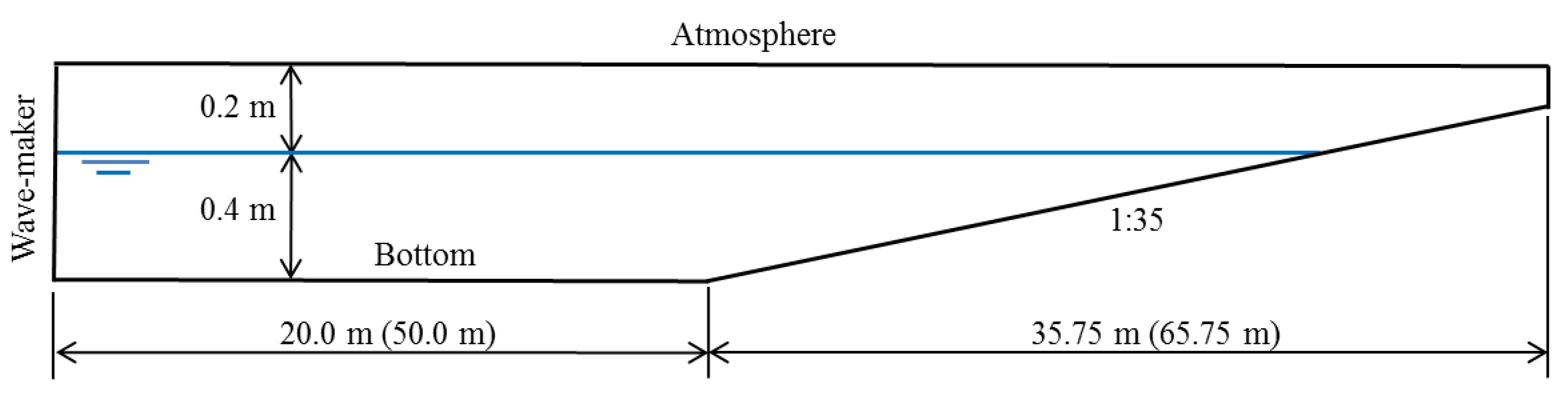
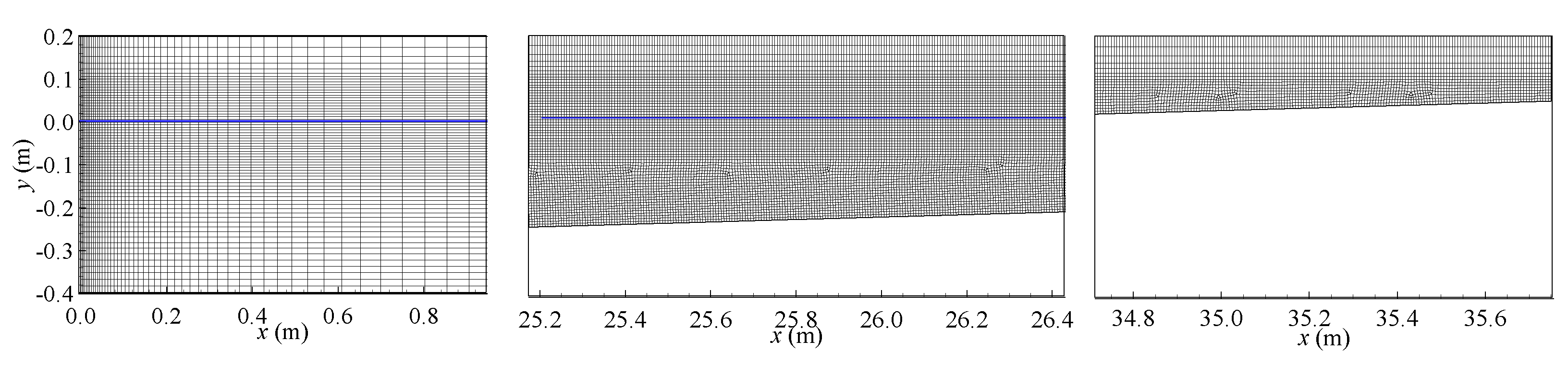
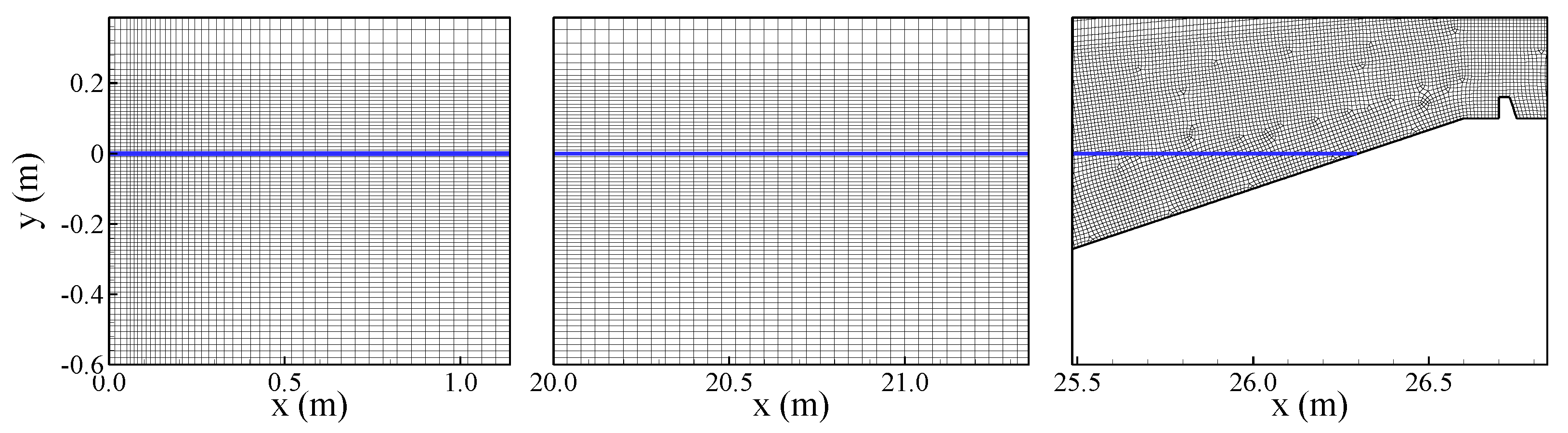
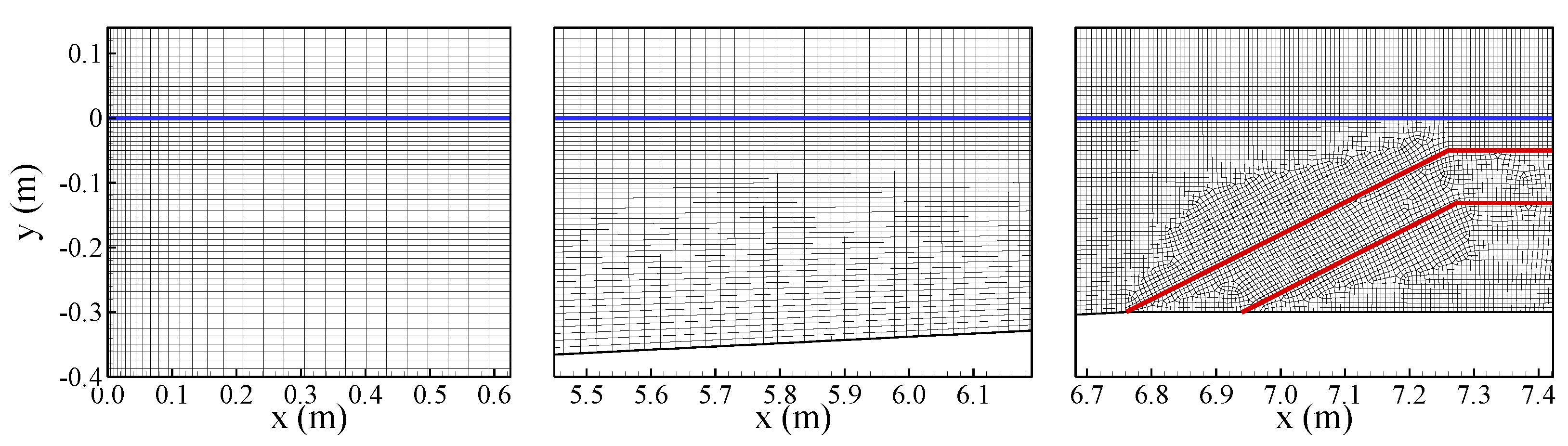
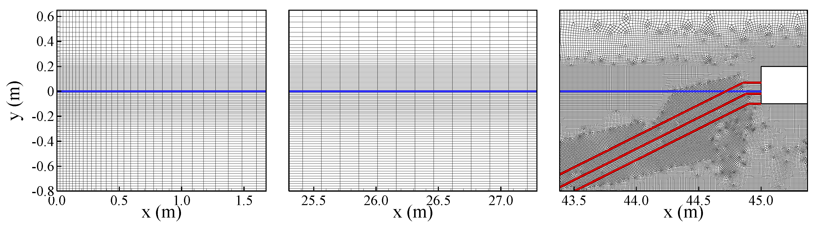
Spatial discretization. Computational meshes of wave flumes with coastal structures have, at least, two main zones with different characteristics: the propagation wave zone and the zone around the structure. In the former, a structured regular mesh is used, in which the free surface is well behaved, and the mesh must be refined around it. Generally, in this zone, the boundary layer on the bottom does not significantly influence the water flow and, consequently, its spatial discretization is not important and does not require a fine resolution. Mesh resolution for accurate wave propagation is defined as follows: in the horizontal direction, 70 cells per wavelength are employed; in the vertical direction, the mesh follows the rule of 20 cells per wave height, in the zone of variation of free surface flow, and it is stretched to the bottom and top of the flume [60,61,62,63,64,65,66]. In zones around and inside the coastal structure, the flow has a different and complex behavior and, generally, regular cells are recommended with an aspect ratio close to 1 [9,10,11].

(e)

Time discretization. A variable time step is used for time integration, in which the maximum value is Tp/600 (Tp is the peak period for a random wave and the wave period for regular waves) and the minimum one is 30 times smaller than the maximum time step [52]. Six non-linear iterations per time step enable the reduction of residue by at least two orders of magnitude which are enough to obtain good accuracy in wave propagation and wave–structure interaction [52,53,60,61,62,63,65].

3. Previous Analysis of Turbulence Models and Mesh Dependency

It is well known that an accurate solution in numerical modeling is partly due to the quality of the mesh, verified by a classical mesh dependency study. However, the free surface flow modeling in cases with wave propagation involves additional degrees of difficulties. One major and known difficulty comes from the decay of the wave height for longtime modeling of wave propagation in a long numerical wave flume when conventional turbulence models are used. Larsen and Fuhrman [14] showed that only adapted turbulence models can maintain characteristics of the wave during the propagation by avoiding the growth of turbulent kinetic energy and eddy viscosity. This is achieved by new and stable closure models proposed by Larsen and Fuhrman [14]. Nevertheless, in these conditions, almost same results can be obtained by the k-ε NLS turbulence model [5,42] for wave propagation and wave overtopping, which are two cases analyzed in Section 3.1. In Section 3.2, a classical convergence study with mesh refinement is performed for the complex case of wave overtopping on an impermeable sea dike with a crown-wall using the k-ε NLS turbulence model.

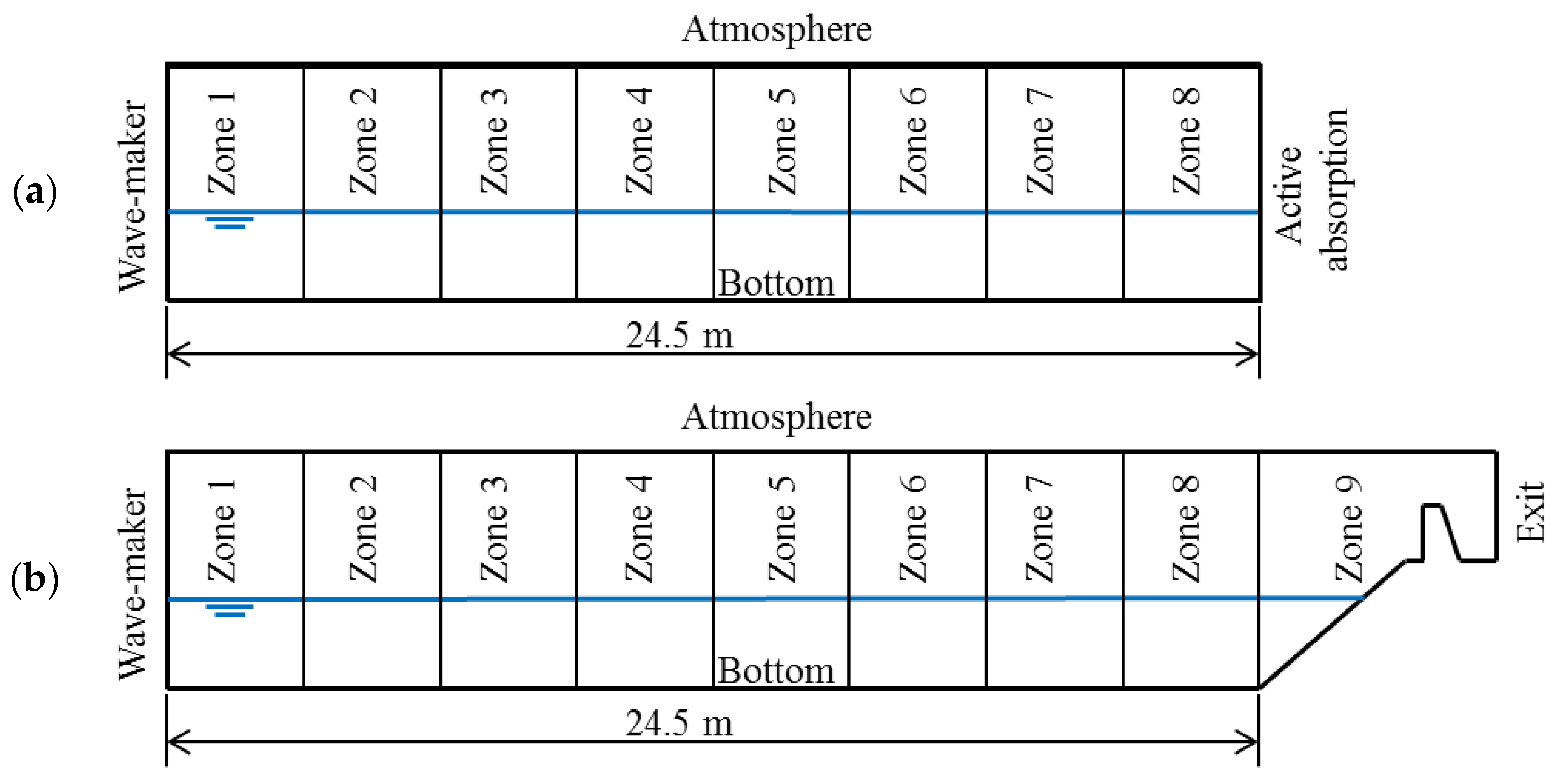
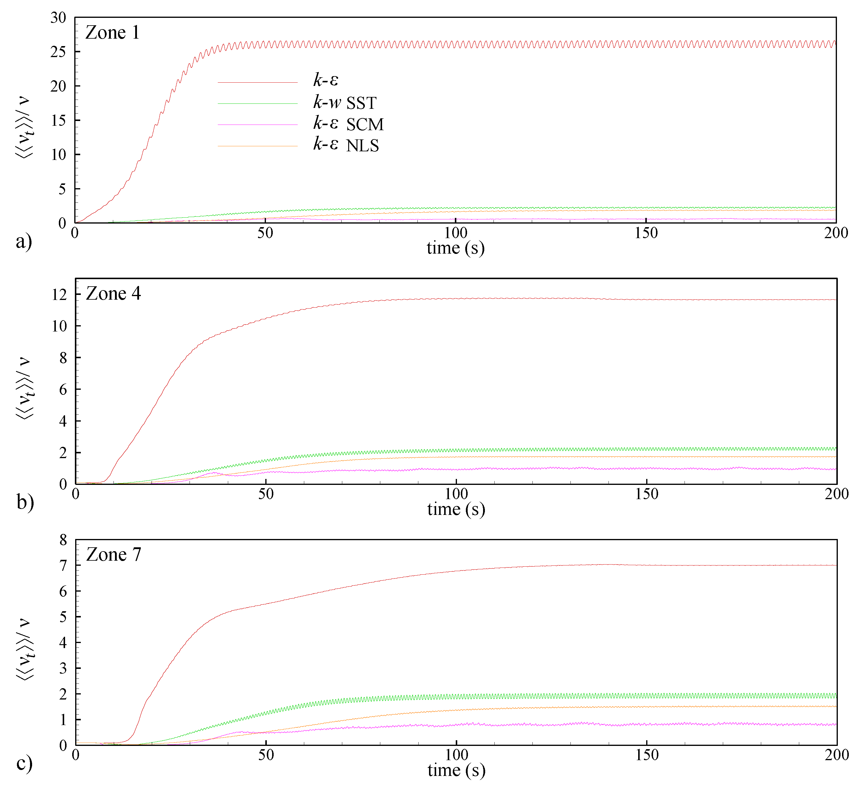
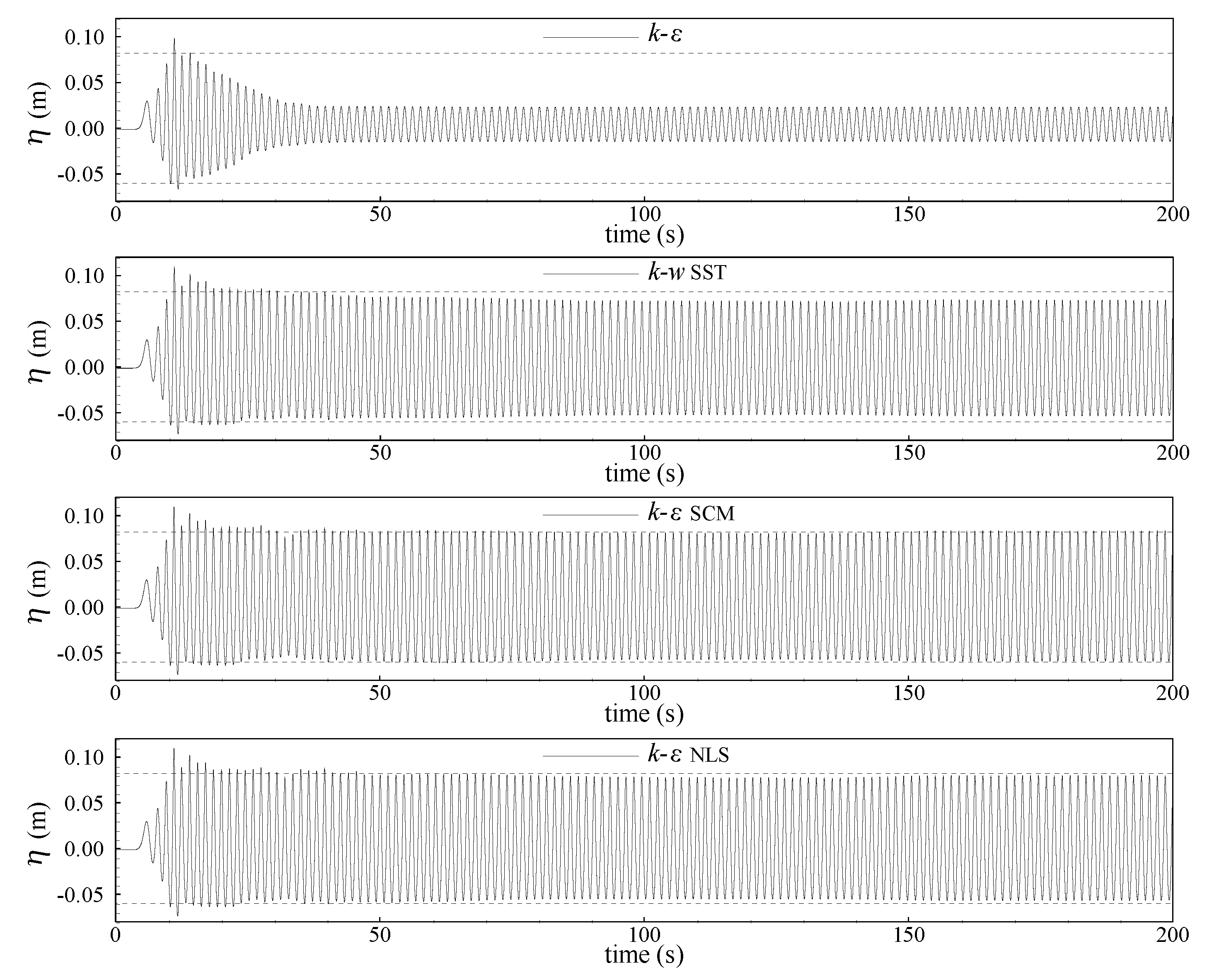
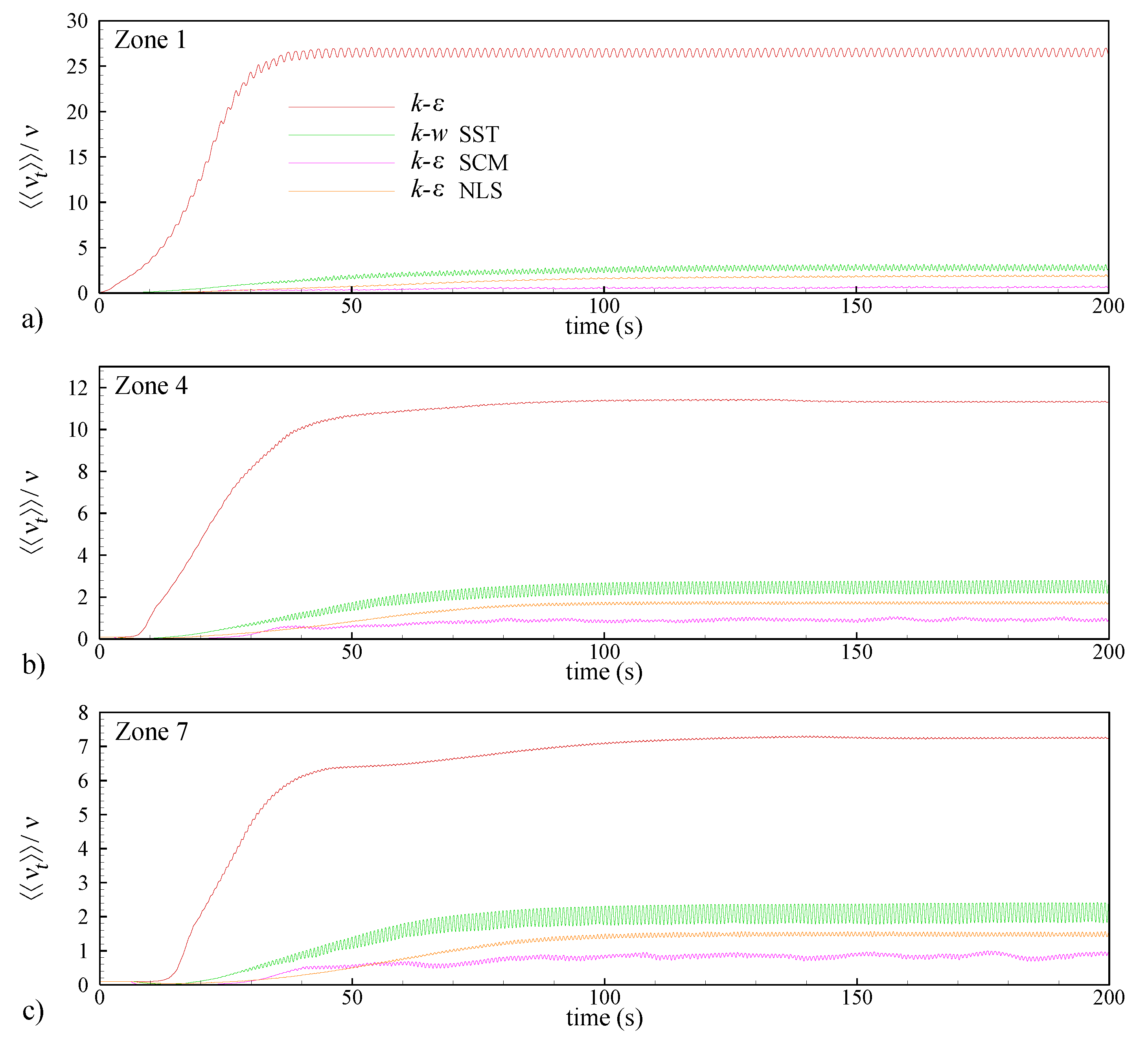
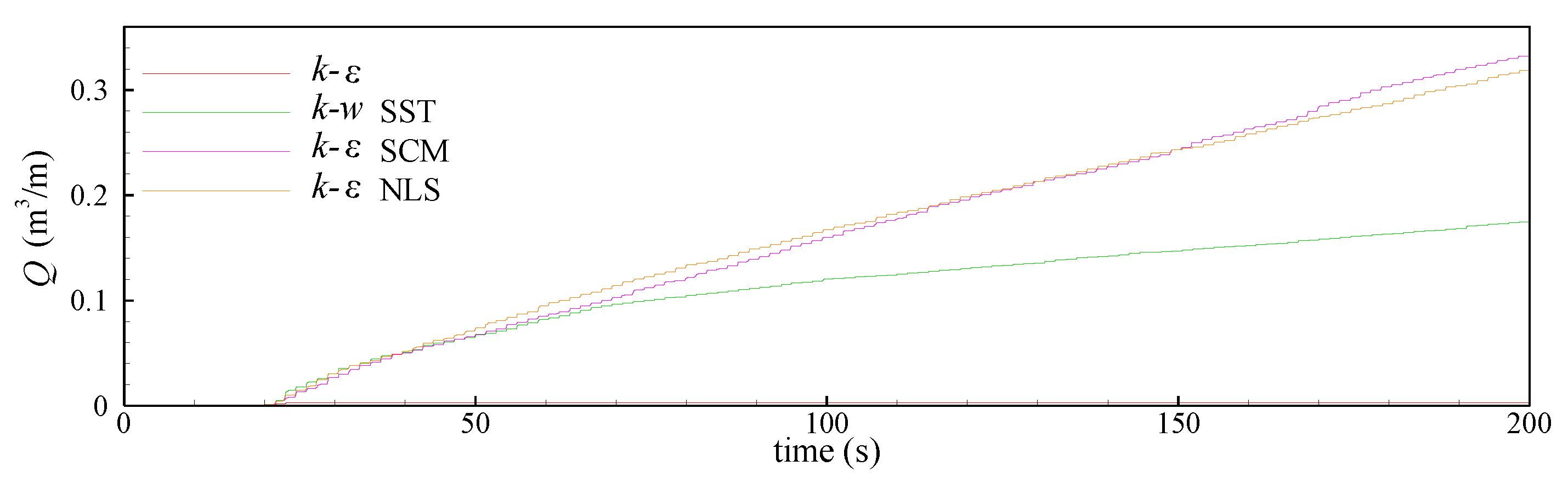
3.1. Analysis of the Grow of Eddy Viscosity along a Flume in Longtime Simulation

In order to follow the analysis carried out by Larsen and Fuhrman [14], highlighting the absolute necessity of using more adapted turbulence models avoiding the growth of eddy viscosity for free surface flows modelling, four turbulence models, shown in Section 2, are tested for wave propagation over a horizontal bottom wave flume and wave overtopping on an impermeable sea dike with a crown-wall [18]. For both configurations, the incident wave is regular, with T = 1.5 s and H = 0.16 m, being considered moderately non-linear in intermediate-depth water. The horizontal wave flume length is 8 L, where L is the wave length, and the simulation time is 300 s, which corresponds to 200 waves. Mesh resolution for both cases follows the recommendations described in Section 2.4, Section 3.2 and Section 4.2.

For analyzing the growth of eddy viscosity in space and time, the spatial average of the non-dimensional eddy viscosity $⟪{\nu }_t⟫/\nu$ is calculated in zones of length L along the flume: ν_t is the kinematic eddy viscosity and ν is the kinematic viscosity of the fluid. For the wave propagation case, the horizontal wave flume is divided in eight zones of length L and an active absorption is imposed at the end of the flume. Figure 1a shows a sketch of the flume and the position of the eight zones. For the wave overtopping case, a ninth zone is added, which includes the sea dikes, crown-wall and dike crest. Figure 1b shows a sketch of the wave flume for this case and the division of the flume by nine zones. An outflow condition is imposed at the end of the flume. These analyses differ slightly from Larsen and Fuhrman [14], in which the growth of eddy viscosity along the time in a computational domain of single wavelength using periodic lateral boundaries is calculated for simulating a simple progressive wave train.

The wave propagation over a horizontal bottom wave flume is firstly analyzed (Figure 1a). Figure 2 shows the time series of $⟪{\nu }_t⟫/\nu$ for three zones along the flume: zone 1, in the vicinity of the wave-maker; zone 4 and zone 7, in the middle and near the end of the flume, respectively. Figure 3 shows the time series of the free surface elevation in the middle of the wave flume, at 12.25 m from the wave-maker, for the four turbulence models (k-ε, k-ω SST, k-ε NLS and k-ε SCM). The dash-lines indicate the mean wave crest and trough obtained by the k-ε NLS turbulence model, which is considered as a reference.

Figure 2 clearly shows that the standard k-ε turbulence model results in a significant and rapid growth of eddy viscosity, which produces a non-physical decay of free surface elevation along the time, with a wave height reduction of 75% compared to the wave height obtained by the k-ε NLS turbulence model. The k-ω SST turbulence model exhibits a slightly greater growth of eddy viscosity than those of k-ε SCM and k-ε NLS ones. It results in a little decay of free surface elevation (Figure 3), which seems to indicate that the standard k-ω SST turbulence model does not include a stable closure model. The wave height reduction is 12% compared to that obtained by the k-ε NLS turbulence model. Finally, k-ε SCM and k-ε NLS turbulence models avoid unphysical behaviors of the free surface elevation and are able to simulate a nearly constant form wave propagation over long durations and along the wave flume. The value of $⟪{\nu }_t⟫/\nu$ is slightly smaller than 1.0 for the k-ε SCM turbulence model and around 1.7 for the k-ε NLS turbulence model on the three zones analyzed. A slight difference of the wave height, around 3%, can be noted between both models, which can be related to the methodologies of each model and minor numerical diffusion associated with numerical schemes.

The second case analyzed involves wave breaking and wave overtopping over an impermeable dike (Figure 1b). Figure 4 shows the time series of $⟪{\nu }_t⟫/\nu$ for the four turbulence models and three zones along the flume: zone 1, in the vicinity of the wave-maker; zone 4 and zone 7, in the middle and near the toe of the sea dike, respectively. The case corresponds to the configuration W6S0 of Tuan and Thin [18], in which there is a vertical wall 0.06 m high on the dike crest (W) without a promenade (S is 0 cm) (see Section 4.2 for more details). Figure 5 presents the time series of the wave overtopping discharge.

Figure 4 shows that the standard k-ε turbulence model results in a significant and rapid growth of eddy viscosity, similar to that observed in the wave propagation case. The k-ω SST turbulence model shows a slightly greater growth of eddy viscosity than both k-ε SCM and k-ε NLS, with a value of $⟪{\nu }_t⟫/\nu$ slightly smaller than 1.0 for the k-ε SCM turbulence model and around 1.7 for the k-ε NLS turbulence model. The wave overtopping discharge of the turbulence models (Figure 5) shows drastic differences. Since the significant growth of eddy viscosity using the standard k-ε turbulence model implicates a significant and unphysical decay of free surface elevation, wave overtopping discharge is completely wrong, being null in the time interval from 120 to 198 s. The other turbulence models show the same trend up to 50 s. However, k-ω SST turbulence models exhibit a decay of wave overtopping discharge after this instant, due to the growth of eddy viscosity, as demonstrated in the wave propagation case. The average wave overtopping discharge is smaller than the experimental one, 1.58 l/s/m [18], being 0.563 l/s/m for the k-ω SST turbulence model, i.e., 67% smaller than the experimental value. Only k-ε SCM and k-ε NLS turbulence models show a regular and nearly constant trend of wave overtopping discharge along the time, since both models avoid the non-physical growth of the eddy viscosity. The average wave overtopping discharges of k-ε SCM and k-ε NLS turbulence models are rather similar, at 1.727 and 1.672 l/s/m, respectively, with a difference of only 3%. Both results are slightly greater than the experimental one.

These two tests demonstrate how the standard k-ε turbulence closure model, widely used for modeling wave propagation and wave–structure interaction, can lead to severely over-predicted eddy viscosity levels, causing the decay of the free surface elevation and an under-estimated wave overtopping discharge. The k-ω turbulence model shows a correct behavior and allows accurate results for wave propagation and wave overtopping to be obtained, but only for short simulations. For long simulations, the growth of eddy viscosity, even if it remains smaller than observed in the k-ε turbulence model, leads to the decay of the free surface elevation and severe under-estimation of the wave overtopping discharge. On the contrary, two completely different models, k-ε SCM and k-ε NLS turbulence ones, based on the stabilized closure model and non-linear Reynolds stress tensor, respectively, allow avoidance of unphysical behaviors and modeling wave propagation, and a nearly constant wave overtopping discharge over long durations. Therefore, turbulence models k-ε SCM and k-ε NLS are suitable for modeling wave propagation, wave–structure interactions and wave overtopping. Nevertheless, in cases of short flumes, in which the short propagation distance limits the extent of the turbulence over-production, and short time simulations, the growth of the eddy viscosity causing the waves decay could not occur, as referred by Larsen and Fuhrman [14] and verified by the authors.

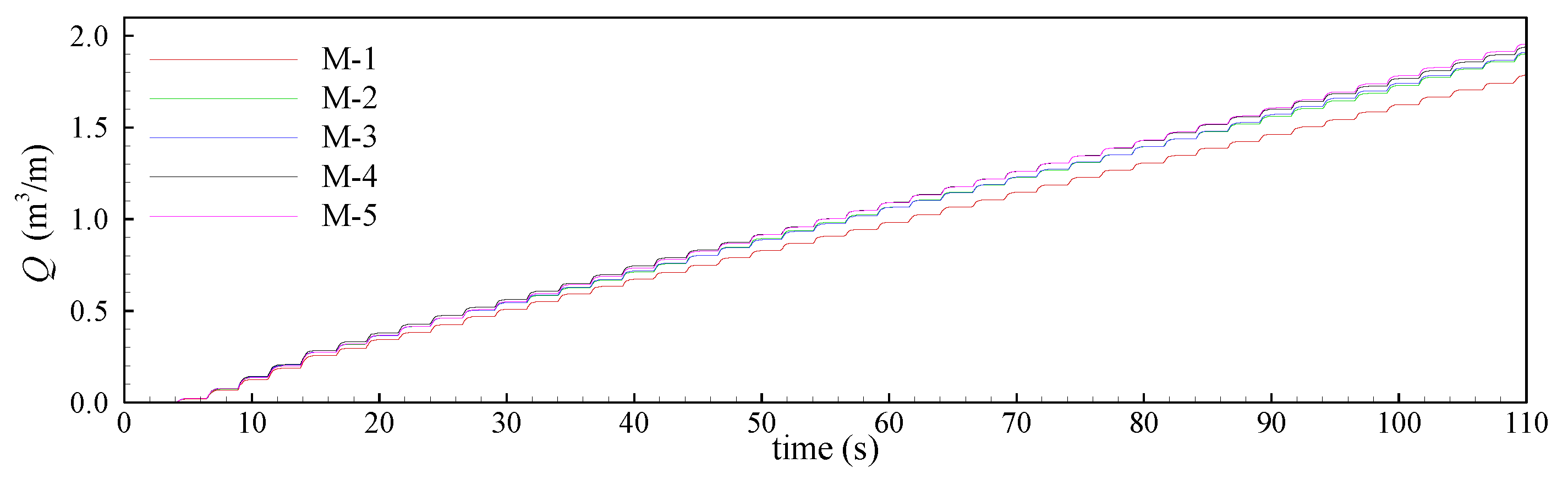
3.2. Mesh Dependency Analysis

Mesh dependency analysis is carried out for the case W6S0 of Tuan and Thin [18], which is a representative case of the wave over coastal structure that involves wave breaking and overtopping. This case corresponds to a vertical wall on the dike crest with 0.06 m height (W) without a promenade (S is 0 cm) (see Section 4.2 for more details). The impermeable model dike is 0.70 m height, with a seaward slope 1/3 and 0.10 m of the freeboard. A regular incident wave with 2.5 s period and 0.24 m high is generated. The numerical wave flume length is reduced for the mesh dependency analysis, in which the length from the wave-maker to the toe of the seaward slope is 6.0 m, i.e., around two wave lengths.

Table 1. Mesh characteristics in the mesh dependency analysis.

Mesh	dl (×10−2 m)	Number of Cells
M-1	1.5 × 1.5	26,521
M-2	1.0 × 1.0	29,805
M-3	0.75 × 0.75	33,351
M-4	0.5 × 0.5	39,226
M-5	0.4 × 0.4	45,018

shows characteristics of the five meshes used in this study. Meshes are unchanged in the wave propagation part of the fume, i.e., from the wave-maker to the toe of the sea dike ramp, following the recommendations described in Section 2.4. The mesh refinement is carried out only in the vicinity of the structure, from the toe of the ramp to the end of the wave flume, using an unstructured mesh with regular cells of characteristic length dl, i.e., with aspect ratio close to 1 (see Section 4.2 for more details). The cell number varies from 26,521 to 45,018 for the coarser to finer meshes (Table 1), which corresponds to a reduction of dl from 1.5 to 0.4 cm in the vicinity of the structure, i.e., the cell area is reduced by a factor of 14. The k-ε NLS turbulence model is used for the mesh dependency analysis, although the k-ε SCM turbulence model could also be used.

Figure 6 presents a time series of the wave overtopping discharge, Q, for the five meshes.

Table 2. Average wave overtopping discharge for meshes M-1 to M-5.

Mesh	Average Wave Overtopping Discharge (m3/m)	Relative Error (%) to Finer Mesh M-5
M-1	16.024	6.96
M-2	16.867	2.07
M-3	17.015	1.21
M-4	16.918	1.77
M-5	17.223	-

shows the average wave overtopping discharge, calculated over the time interval from 60 to 110 s, i.e., 20 wave periods, and its relative error comparing to the finer mesh M-5. It can be seen that wave overtopping discharge has the same trend for meshes M-2 to M-5, with only small differences. The coarser mesh M-1 shows a slightly different behavior. The averaged wave overtopping discharge difference between meshes M-2 to M-4 and the finer mesh M-5 is small, around or inferior to 2%, and very similar for mesh M-2 and M-4. Since mesh M-2 gives similar values to mesh M-4, mesh resolution used for mesh M-2 seems to be a good choice compared to conducted simulations, and it is adopted for simulations of Tuan and Thin [18] in Section 4.2.

Different to the well behaved case of the wave propagation on a flume, there is no possibility of recommending element sizes in the vicinity of coastal structures, based on dimensional characteristics of the problem, due to the complexity of involved phenomena. Therefore, in other cases presented in Section 4, element sizes are equal or close to those used by the authors in their investigations, so that comparison of results is possible.

4. Results and Discussion

Methodologies implemented in the FLUENT^® numerical model are validated by comparing numerical results with experimental and numerical ones in the literature. Four configurations are tested: wave breaking over an impermeable beach of Ting and Kirby [6], wave overtopping on impermeable sea dikes with crown-walls of Tuan and Thin [18], wave interaction with a porous low-crested rubble-mound breakwater of Garcia et al. [33] and wave overtopping on a rubble mound breakwater of Losada et al. [15]. The quantitative analysis of numerical results is carried out using the Bias statistical parameter [67] and the NRMSE (normalized root mean square error), which are obtained comparing numerical results with those of the reference. Bias is defined as follows:

$$Bias=\frac{{{\displaystyle \sum }}_i^n\left(s_i-m_i\right)}{n}$$

(49)

where s_i are values obtained by the numerical simulation, m_i are reference values and n is the sample size. NRMSE, as a percentage, is given by:

$$NRMSE=100\sqrt{{\displaystyle \sum }_i^n\frac{{\left(s_i-m_i\right)}^2}{n}}/\overline{m}$$

(50)

where $\overline{m}$ is the average of the reference values.

4.1. Spilling and Plunging Wave Breakers on an Impermeable Beach

Physical experiments developed by Ting and Kirby [6] are used to validate numerical models in cases of spilling and plunging wave breaking on an impermeable bottom beach. It consists of a flume 0.4 m deep with a slope (1:35) at one end. The origin of the horizontal coordinate (x) considered by Ting and Kirby [6] is 0.7 m from the beginning of the slope. Incident waves with T = 2 s and H = 0.125 m (spilling) and T = 5 s and H = 0.128 m (plunging) are generated in the wave-maker by using the Fourier theory. A sketch of the computational domain is shown in Figure 7, in which dimensions in parenthesis represent the plunging case. The horizontal wave flume length is 20.0 m (5.2 L) and 50.0 m (4.7 L), respectively. The mesh resolution follows the recommendations described in Section 2.4 and 3.2, and an unstructured mesh with regular cells with a grid resolution close to 0.0063 × 0.0063 m (aspect ratio close to 1) is used in the slope region (Figure 8). The total number of cells is around 115,157 and 118,976 for the spilling and plunging cases, respectively.

Figure 9 shows maximum and minimum wave height envelopes and mean water level obtained by using turbulence models k-ε, k-ω SST, k-ε NLS and k-ε SCM for the spilling case (black dashed line in Figure 9 indicates the still water level). Results are compared with experimental ones of Ting and Kirby [6] at instants from 80 to 90 s. Clearly, the standard k-ε turbulence model is highly dissipative and, consequently, it systematically underestimates the wave height envelopes and leads to unphysical behaviors. The other turbulence models have similar results, with slightly better ones reached by the k-ε NLS turbulence model, meanly because it accurately follows the breaking zone.

Table 3. Bias and NRMSE of wave height for spilling and plunging cases and k-ε, k-ω SST, k-ε NLS and k-ε SCM turbulence models.

	T = 2 s, H = 0.125 m		T = 5 s, H = 0.128 m
	Bias (cm)	NRMSE (%)	Bias (cm)	NRMSE (%)
k-ε	−4.97	59.2	−3.58	35.4
k-ω SST	−0.38	8.4	0.05	10.6
k-ε NLS	0.25	6.5	0.80	11.9
k-ε SCM	−0.01	9.7	0.75	10.1

shows the Bias and NRMSE of wave height obtained by turbulence models. The lowest Bias is −0.01 cm of the k-ε SCM turbulence model, and the lowest NRMSE is 6.5% of the k-ε NLS turbulence model.

Figure 10 shows maximum and minimum wave height envelopes and mean water level by using turbulence models k-ε, k-ω SST, k-ε NLS and k-ε SCM at instants from 70 to 90 s for the plunging case (black dashed line in Figure 10 indicates the still water level). As the spilling case, the k-ε turbulence model significantly underestimates the wave height envelopes, leading to unphysical behavior, and the other turbulence models have similar results, in which the maximum wave height envelopes are overestimated before the wave breaking zone. Although the k-ω SST turbulence model has the lowest Bias, 0.05 cm, it occurred because there is a higher underestimation of the maximum wave height envelope in the wave breaking zone, which compensates the overestimation before this zone. NRMSE of all turbulence models are similar, from 10.1 to 11.9%, except the k-ε one (Table 3).

In summary, the k-ω SST, k-ε NLS and k-ε SCM turbulence models show similar results for spilling and plunging wave breakwaters, while the k-ε turbulence model leads to unphysical behaviors.

4.2. Wave Overtopping on Sea Dikes with Crown Walls

In order to evaluate the capability of the model to simulate wave overtopping, physical experiments and numerical results obtained by Tuan and Thin [18] are used. Among the set of experiments presented by Tuan and Thin [18], the model dike was smooth and impermeable, using a height of 0.70 m and a 1/3 seaward slope (Figure 11). The vertical wall on the dike crest is 0, 4, 6 and 9 cm height (W) and the promenade width (S) is 0, 0.10 and 0.20 m. Freeboard is 0.10 and 0.15 m for regular and random wave tests, respectively. The computational domain has the same dimensions as Tuan and Thin [18], with 24.5 m from the inflow waves at the seaward boundary and the dike toe. It is important to emphasize that the physical wave flume is 45 m long, and Tuan and Thin [18] used a recorded time-series from the wave gauge at 24.5 m seaward of the structure to generate the incident waves at the boundary, whereby the free surface and the velocity components are prescribed. However, theoretical values of wave period and wave height are used in the present study to generate the incident wave in the static paddle. Fourier waves are generated for both regular wave cases (T =1.5 s, H = 0.16 m and T = 2.5 s, H = 0.24 m), and a JONSWAP-type spectrum is considered for two random wave tests (T_p = 2.2 s and H_s = 0.123 and 0.126 m). The mesh resolution follows the recommendations described in Section 2.4 and Section 3.2, and an unstructured mesh with regular cells with a grid resolution close to 0.01 × 0.01 m, i.e., aspect ratio close to 1, is used in the proximity of the dike and the vertical wall (Figure 12). The total number of cells is around 70,000, varying with the length of the promenade and the wall height. The k-ε NLS and k-ε SCM turbulence models are used for this application, since both models allow accurate results of average wave overtopping discharges to be obtained, different to the standard k-ε and k-ω SST turbulence models, as verified in Section 3.1.

Average wave overtopping discharges predicted by the numerical model compared with the experimental and numerical results of Tuan and Thin [18] are shown in

Table 4. Average wave overtopping discharge of regular (RE) and random (IR) waves: experimental and numerical from Tuan and Thin [18] and numerical predictions for k-ε NLS and k-ε SCM turbulence models.

Case	Regular Waves				Average Wave Overtopping Discharge (l/s/m)
					Tuan and Thin [18]		Turbulence Model
	W (cm)	S (cm)	H (m)	T (s)	Exp.	Num.	k-ε NLS	k-ε SCM
REW0S0_1	0	0	0.16	1.5	5.26	5.08	6.74	7.51
REW0S0_2	0	0	0.24	2.5	21.05	21.23	27.57	27.97
REW0S4_1	4	0	0.16	1.5	2.28	2.54	3.05	3.58
REW0S4_2	4	0	0.24	2.5	21.75	20.91	20.77	22.50
REW4S10_1	4	10	0.16	1.5	1.14	2.09	2.73	3.24
REW4S10_2	4	10	0.24	2.5	19.82	18.12	20.46	21.09
REW4S20_1	4	20	0.16	1.5	0.70	0.98	2.75	2.68
REW4S20_2	4	20	0.24	2.5	18.42	18.33	19.69	20.49
REW6S0_1	6	0	0.16	1.5	1.58	1.65	1.77	1.78
REW6S0_2	6	0	0.24	2.5	17.02	16.10	17.09	18.49
REW6S10_1	6	10	0.16	1.5	1.14	1.01	2.13	2.37
REW6S10_2	6	10	0.24	2.5	15.61	16.60	17.69	18.14
REW6S20_1	6	20	0.16	1.5	0.19	0.34	1.49	1.71
REW6S20_2	6	20	0.24	2.5	13.51	17.12	16.11	17.03
REW9S0_1	9	0	0.16	1.5	1.32	0.51	0.69	0.58
REW9S0_2	9	0	0.24	2.5	14.39	13.29	10.59	12.34
REW9S10_1	9	10	0.16	1.5	0.21	0.21	1.01	1.28
REW9S10_2	9	10	0.24	2.5	13.51	8.94	13.46	14.99
REW9S20_1	9	20	0.16	1.5	0.04	0.05	0.34	0.14
REW9S20_2	9	20	0.24	2.5	10.18	8.94	10.44	12.51
Case	Random waves
	W (cm)	S (cm)	H (m)	Tp (s)	Exp.	Num.	k-ε NLS	k-ε SCM
IRW6S10	6	10	0.123	2.2	0.224	0.281	0.145	0.155
IRW9S10	9	10	0.126	2.2	0.096	0.073	0.065	0.078

for regular (RE) and random (IR) waves. Figure 13 shows the present and Tuan and Thin (2014) numerical results versus the experimental ones. Numerical and experimental average wave overtopping discharges in Tuan and Thin [18] are calculated from around 10 waves for regular waves and 1000 waves for random waves. In the present study, overtopping discharges for regular waves are recorded from the 30th and 50th waves, whereby the periodic stationary wave–structure interaction flow is obtained. For random waves, 1000 waves are recorded, i.e., 1000T_p, according to Tuan and Thin [18]. The present average wave overtopping discharge is obtained from the water volume flow rate monitored after the vertical wall.

It can be seen from Table 4 and Figure 13 that both turbulence models present globally higher average wave overtopping discharges than experimental and numerical results obtained by Tuan and Thin [18], especially for small overtopping discharge. Bias parameters of the k-ε NLS turbulence model are 0.87 and 0.86 compared to experimental and numerical results of Tuan and Thin [18], respectively; conversely, those of the k-ε SCM turbulence model are 1.56 and 1.55, respectively. The k-ε SCM turbulence model exhibits an average wave overtopping discharge 6.1 and 9 times greater than experimental values for the cases REW9S10_1 and REW6S20_1, respectively, both with small wave overtopping discharge. Both cases present a larger difference compared to experimental values. Using the k-ε NLS turbulence model, both cases exhibit an average wave overtopping discharge 4.8 and 7.8 times greater than experimental values, respectively, slightly smaller than those obtained by using the k-ε SCM turbulence model. Nevertheless, the average wave overtopping discharge is well predicted in several cases using the k-ε NLS turbulence model, such as in REW6S0 and REW9S10.

The NRMSE of average wave overtopping discharges, for the set of cases presented in Table 4, is 38.6 and 34.4% for the k-ε SCM and k-ε NLS turbulence models, respectively. Results obtained using the k-ε NLS turbulence model are in better accordance with experimental data than those predicted by the k-ε SCM turbulence model. However, NRMSE of both models is larger than NRMSE of Tuan and Thin [18], which is equal to 23.2%. Nevertheless, the comparison of average wave overtopping discharges greater than 10 l/s/m shows that both turbulence models and Tuan and Thin [18] present the same order of magnitude of NRMSE and accuracy: NRMSE is 17.9% for k-ε SCM, 16.1% for k-ε NLS, and 14.5% for Tuan and Thin (2014). In cases when average wave overtopping discharges are smaller than 10 l/s/m, NRMSEs are quite large: 103.7% for k-ε SCM, 83.4% for k-ε NLS, and 30.4% for Tuan and Thin [18]. It is important to emphasize that the wave overtopping discharge is very sensitive to the model, experimentally and numerically, and differences found between present results and those of Tuan and Thin [18] are of the same order of magnitude as reported by Neves et al. [53].

For random waves, it can be noted that average wave overtopping discharges are small. For the case IRW9S10, k-ε SCM and NLS turbulence models and numerical results of Tuan and Thin [18] underestimate the average wave overtopping discharge, with a difference around 20% compared to experimental values, and slightly greater for k-ε NLS turbulence model, at 30%. For the case IRW6S10, k-ε SCM and NLS turbulence models underestimate the average wave overtopping discharge, with differences of 30 and 35%, respectively, compared to the experimental values, while Tuan and Thin [18] overestimates, with a difference of 25%.

Differences in average wave overtopping discharges found among turbulence models can lead to differences in the plunging breaking wave, wave dissipation after wave breaking and, consequently, in the wave overtopping. In addition, differences between k-ε SCM and NLS turbulence models used in this study and those employed by Tuan and Thin [18] could be related to different methods used for wave generation.

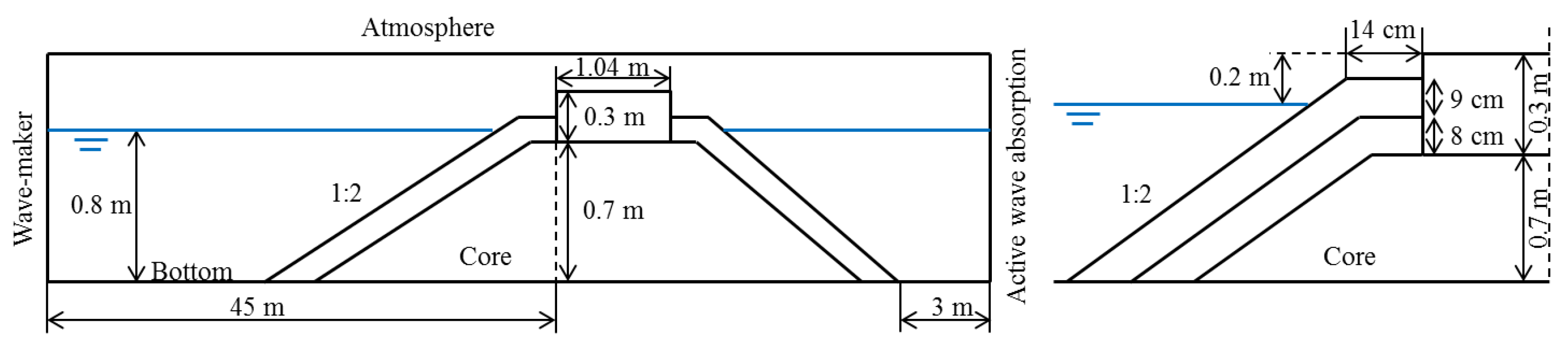
4.3. Wave Interaction with Porous Low Crested Rubble Mound Breakwater

Physical experiments conducted at the University of Cantabria within the framework of the European Union Design of Environmental Low Crested Coastal Defence Structures (DELOS) project are used to validate the numerical model in cases of regular and random waves impinging on low-crested rubble-mound multilayered breakwater. The case is examined by Garcia et al. [33] for regular waves and Lara et al. [34] for random waves by using the VARANS numerical model COBRAS (Cornell Breaking Waves and Structures [24,32]). Among the set of experiments, the low-crested breakwater model with 1.0 m crest width and water depth 0.4 m (freeboard with 5 cm) is tested. Figure 14 shows the sketch of the computational domain, which reproduces the general configuration of the tests. The low-crested structure is made of two porous layers of different hydraulic properties above a bottom connected to the bottom of the flume by a 1:20 slope. In the experimental test and mathematical model, the wave flume includes a flow recirculation system aimed at preventing water piling-up in the leeward side of the low-crested structure, due to the rear absorbing 1:20 slope beach at the end of the flume. In COBRAS, wave generation is carried out using a source function with a sponge-layer method used to absorb the waves that propagate in the opposite direction to the zone of interest. In the present numerical wave flume, a static wave-maker with active wave absorption, located at 4.76 m from the toe of the 1:20 bottom flume slope, generates the incident wave at the inlet flow boundary. An active wave absorption is used at the end of the flume which avoids using a flow recirculation system to maintain the mean water level in the leeward side of the low-crested structure. Fourier waves are generated for both regular incident wave cases (T =1.6 s, H = 0.07 and 0.10 m) and a TMA-type spectrum, with a γ parameter equal to 3.3 and cutoff frequencies 0.16 and 1.00 Hz [34], is considered for both random wave tests (T_p = 2.4 and 3.2 s with H_s = 0.10 m). Values of the linear, α_E, and nonlinear, β_E, coefficients governing the flow inside the porous media have been kept equal to those presented by Garcia et al. [33] for regular waves (model calibration was carried out using wave conditions: h = 0.40 m, H = 0.07 m, T = 1.6 s). For random waves, α_E is taken to be equal to 1000 for both armour layers (n = 0.53, D₅₀ = 0.0387) and core (n = 0.49, D₅₀ = 0.0118) and β_E equal to 0.8 and 1.2, respectively, according to Lara et al. [34]. The mesh resolution follows recommendations described in Section 2.4 and Section 3.2, and an unstructured mesh with regular cells with grid resolution close to 0.0035 × 0.0035 m, i.e., aspect ratio close to 1, is used in the proximity of the low-crested structure, inside and outside the porous layers (Figure 15). The total number of cells is around 97,000. Standard k-ε, k-ε NLS and k-ε SCM turbulence models are used for this application, since they include source terms to take into account the effect of turbulence inside the porous media, which it is not the case of the k-ω SST turbulence model.

Similar to Garcia et al. [33] for regular incident waves, numerical results from 10 waves, counted from 60 s of simulation, were analyzed, which ensured stabilized periodic flow conditions. For random waves, 200 waves are simulated for each test, which allows a time series long enough for analysis to be achieved, according to Lara et al. [34].

Figure 16 and Figure 17 show results of maximum and minimum wave height envelopes and mean water level of a regular wave with a period T =1.6 s and wave height H = 0.07 and 0.10 m, respectively. Figure 18 and Figure 19 show results of maximum and minimum wave height envelopes and mean water level of random waves with wave height H_s = 0.10 m and period T_p = 2.4 and 3.2 s, respectively. Numerical results are compared with experimental data of Lara et al. [34] in 11 free surface gauges placed before, over and after the submerged rubble-mound breakwater.

Table 5. Bias and NRMSE of wave height at the 11 sections of measurement for regular and random waves for the k-ε, k-ε NLS and k-ε SCM turbulence models.

	T = 1.6 s H = 0.07 m		T = 1.6 s H = 0.10 m		Tp = 2.4 s HS = 0.10 m		Tp = 3.2 s HS = 0.10 m
	Bias	NRMSE	Bias	NRMSE	Bias	NRMSE	Bias	NRMSE
k-ε	−0.0143	30.1	−0.0246	37.1	−0.0323	39.0	−0.0609	66.0
k-ε NLS	−0.0022	15.4	−0.0028	5.8	0.0028	10.3	−0.0037	9.1
k-ε SCM	−0.0025	15.4	−0.0039	6.9	0.0026	10.2	−0.0056	13.5

presents Bias, Equation (50), and NRMSE, Table 5 presents Bias and NRMSE of the wave height at 11 sections of measurement for regular and random waves for the three turbulence models, of the wave height at 11 sections of measurement for regular and random waves for the three turbulence models.

Table 5 shows that Bias is negative for almost all cases, indicating that the numerical model underestimated the wave heights. Figure 16, Figure 17, Figure 18 and Figure 19 show that the numerical model using the standard k-ε turbulence model, for the four tests, systematically underestimates the maximum and minimum wave height envelopes, the maximum wave height envelope being significantly more underestimated than the minimum one. NRMSE of the wave height varies from 30.1 to 66.0%. However, the numerical model using k-ε NLS and k-ε SCM turbulence models adequately reproduces the main features of the interaction of regular and random waves with submerged porous breakwater. The whole pattern of maximum and minimum wave height envelopes is accurately predicted: in the zone of the structure crest, the wave breaking, represented by the wave height damping, is correctly reproduced; in the leeward region, the transmission features due to overtopping and flow through the porous structure are also well reproduced. The mean water level variations due to wave breaking can be observed and are well predicted: the mean water level decreases at the offshore side of the breaking point and increases at the onshore side. NRMSE of the wave height varies from 5.8 (T =1.6 s, H = 0.10 m, using k-ε NLS turbulence model) to 18.4% (T = 1.6 s, H = 0.07 m, using k-ε turbulence model). In general, considering the four tests for each turbulence model, the average NRMSE is around 10 to 12%, and the best results are obtained using the k-ε NLS turbulence model. NRMSE on the wave height at 11 sections of measurement is 10.3 and 9.1% for k-ε NLS model, and 10.2 and 13.5% for k-ε SCM, for a random wave test with period T_p = 2.4 and 3.2 s, respectively. These values are in agreement with those obtained by Lara et al. [34] for both random waves, at 9 and 8%, respectively.

4.4. Wave Overtopping of a Rubble Mound Breakwater

In order to evaluate the capability of the models to simulate wave overtopping over a rubble mound breakwater, physical experiments obtained by Losada et al. [15] in the wave flume of the University of Cantabria are used. Figure 20 shows the sketch of the computational domain which reproduces the general configuration of the tests. The breakwater is built of an impermeable caisson, with 1.04 m length and 0.3 m height, installed on the rubble mound foundation. The frontal wall is located at 45 m from the wave-maker. The gravel core foundation, with a 1:2 slope, D₅₀ = 0.01 m and porosity 0.48, is 0.7 m high and covered by two external layers: one layer is gravel with D₅₀ = 0.035 m, and the external layer is gravel with D₅₀ = 0.135 m. The porosity is 0.50 for both layers. The bottom of the flume is horizontal, the still water level is 0.8 m, and the structure freeboard is 0.2 m. In the experimental test and the COBRAS-UC numerical model [33,34], three dissipative ramps were placed at the rear end of the wave flume to absorb the transmitted waves. A source function is used in COBRAS-UC for the wave generation associated with a sponge-layer method to absorb the waves that propagate in the opposite direction to the zone of interest. In the present numerical wave flume, a static wave-maker with active wave absorption generates the incident regular wave (Fourier wave for T = 6 s, H = 0.25 m) at the inlet flow boundary and an active wave absorption is used at the end of the flume. Values of the linear, α_E, and nonlinear, β_E, coefficients governing the flow inside the porous media have been kept equal to those presented in Losada et al. [15] for regular waves (model calibration was carried out using wave conditions: h = 0.80 m, H = 0.10 m, and T = 3 and 5 s). The best parameter values are: α_E = 200 for both the armour layer and core; β_E = 0.8 for the breakwater core; β_E = 1.1 for the small gravel external layer; and β_E = 0.7 for the big gravel external layer. The mesh resolution follows the recommendations described in Section 2.4 and Section 3.2, and an unstructured mesh with regular cells with grid resolution close to 0.01 × 0.01 m, i.e., aspect ratio close to 1, is used in the vicinity of the breakwater, which is the area of interest, inside and outside the porous layers (Figure 21). The total number of cells is around 77,240. The standard k-ε, k-ε NLS and k-ε SCM turbulence models are used for this application, since they include source terms that take into account the effect of turbulence inside the porous media, which is not the case of the k-ω SST turbulence model.

Figure 22 shows the free surface elevation at a wave gauge at 42.5 m from the wave- maker, i.e., located near the toe of the breakwater. Two intervals of time are presented: the first time interval, from 0 to 60 s, corresponds to the beginning of the interaction between the wave and the breakwater; and the second one, from 240 to 300 s, corresponds to the periodic stationary flow. Figure 23 shows the time series of the wave overtopping discharge.

Table 6. Average wave overtopping discharge for k-ε, k-ε NLS and k-ε SCM turbulence models compared to experimental and numerical values of Losada et al. [15].

	Losada et al. [15]		FLUENT
	Exp.	Num.	k-ε	k-ε NLS	k-ε SCM
Average wave overtopping discharge (m3/s/m)	0.0066	0.0063	0.0033	0.0083	0.0084
Relative error (%)	-	4.6	50.0	25.8	27.3

shows the average wave overtopping discharge calculated from 138 to 300 s, i.e., considering 27 wave periods.

It can be seen that both free surface elevation and wave overtopping discharge, for the three turbulence models, are very similar until 60 s. However, wave overtopping discharge slows down using the standard k-ε turbulence model, due to the progressive growth of eddy viscosity which reduces the free surface elevation until reaching a stabilized behavior. This does not occur with both k-ε NLS and k-ε SCM turbulence models, which present the same behavior for free surface elevation and wave overtopping discharge. Both models overestimate the average wave overtopping discharge with a difference related to the experimental result of 26%, whereas the value obtained by the standard k-ε turbulence model is largely underestimated. Differences observed between numerical results and those obtained by Losada et al. [15] can be related to the wave generation and the parameter values of the porous layers, which are equal to those of Losada et al. [15], which may not be the best parameters for the present numerical model, even if the porous medium equations seem the same as the author’s.

5. Conclusions

This paper showed methodologies implemented in a RANS-VoF numerical model, the FLUENT^® numerical model in this case, to simulate interactions between waves and impermeable and porous costal structures, which involve wave breaking and overtopping. Performance of standard k-ε and k-ω SST turbulence models was compared with two modified turbulence models, implemented in the RANS-VoF model, which avoid the growth of the eddy viscosity: the k-ε NLS, developed by Shih et al. [42] and Lin and Liu [5], and k-ε SCM, developed by Larsen and Fuhrman [14]. Equations of momentum and turbulence models were adapted in original numerical model to take into account the porous media of coastal structures.

The performance of k-ε NLS, k-ε SCM and standard k-ε and k-ω SST models were compared in cases with wave breaking (regular waves on an impermeable beach of Ting and Kirby [6]), wave breaking and overtopping (regular and random waves over impermeable sea dikes with crow-walls, proposed by Tuan and Thin [18]), wave on a porous submerged structure (regular and random waves over a low-crested rubble breakwater of Garcia et al. [33] and Lara et al. [34]), and wave overtopping in porous structure (regular and random waves over a rubble mound breakwater of Losada et al. [15]). The main conclusions of these analyses are:

(a)

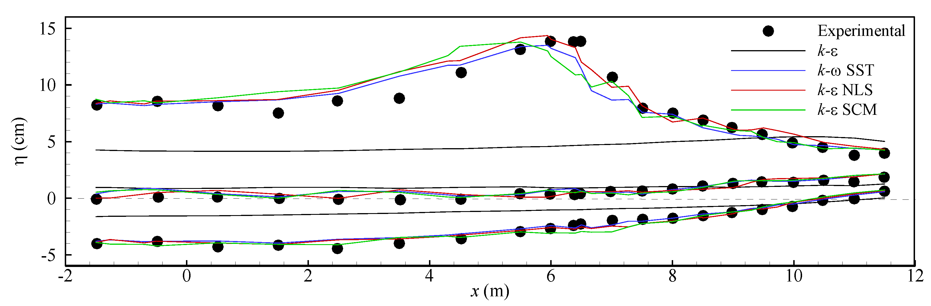
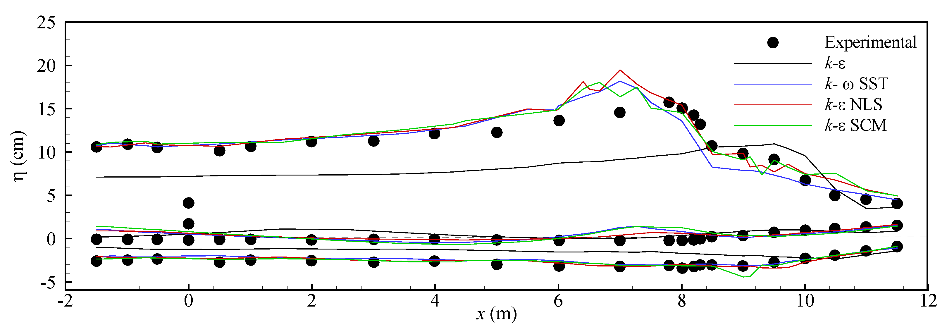
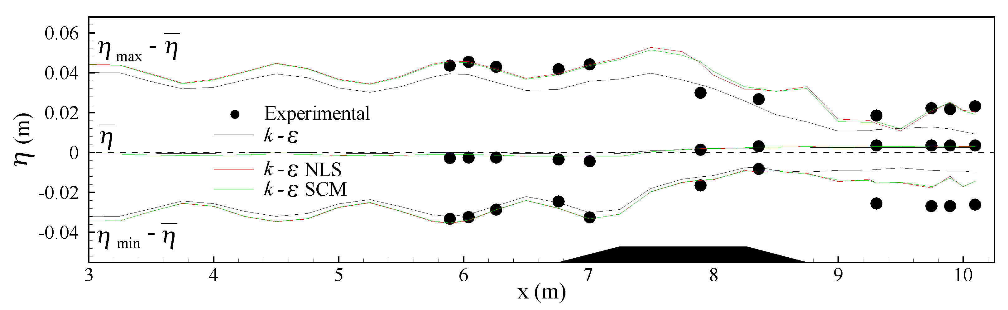
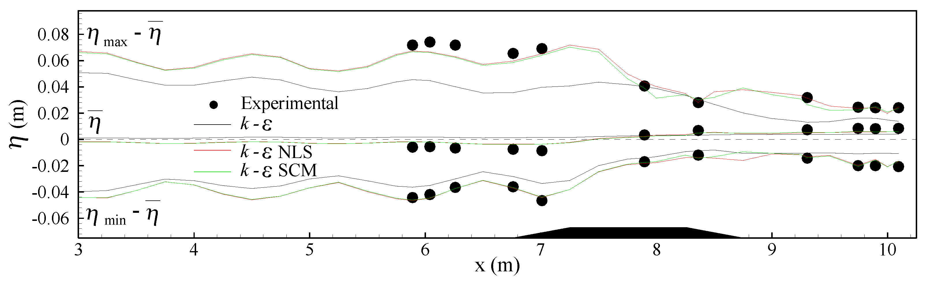
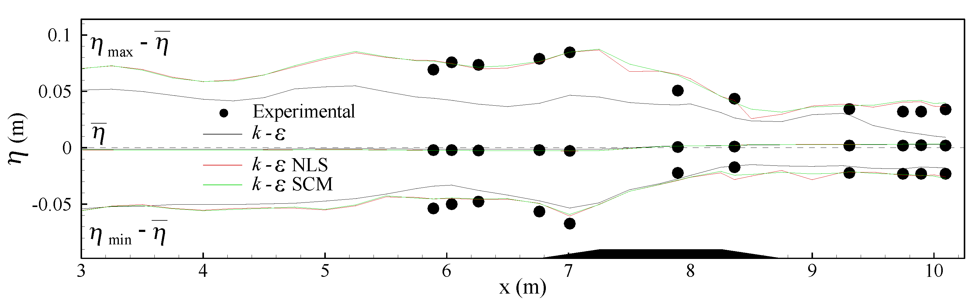
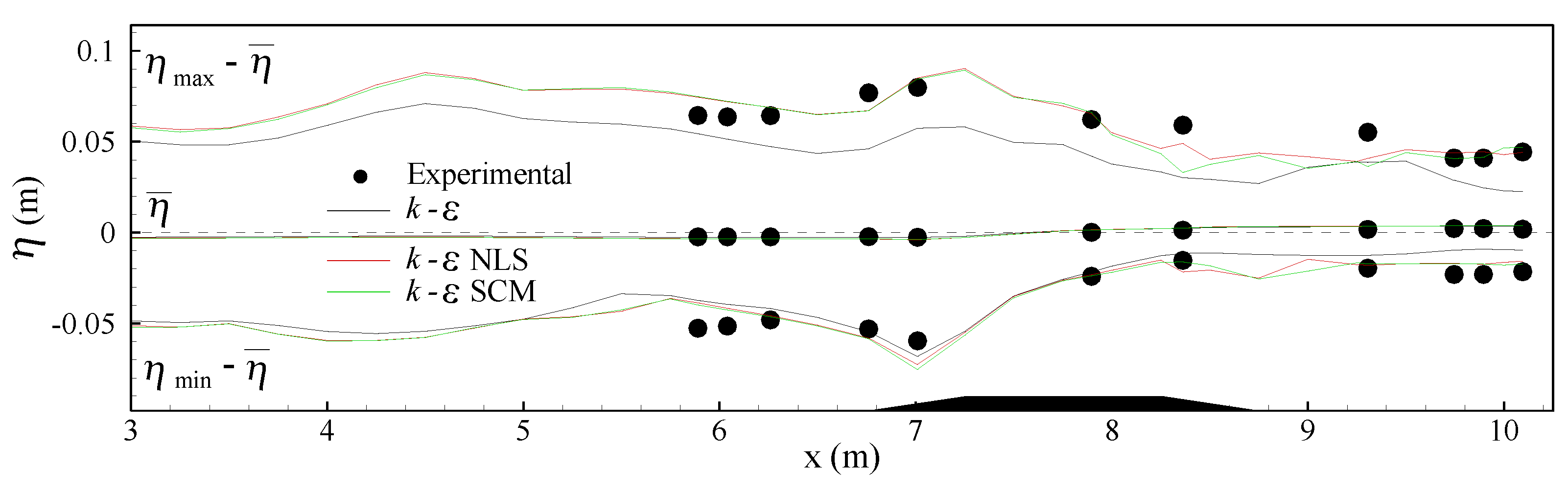
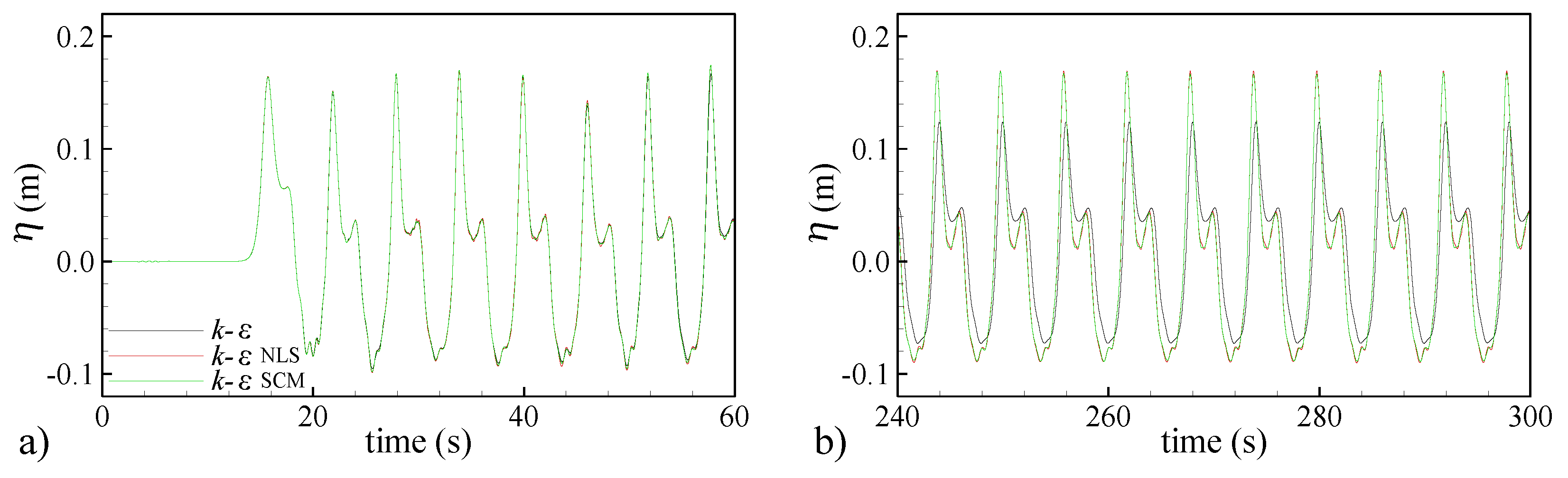
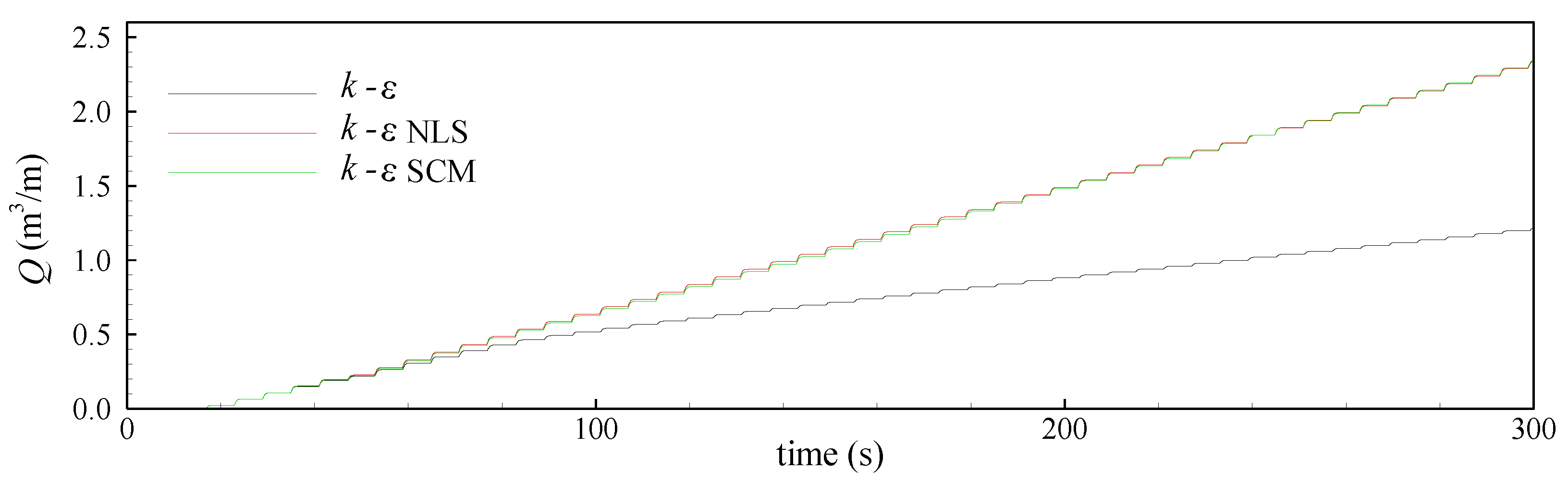
Mainly for longtime simulations in long numerical wave flumes, the standard k-ε turbulence model severely over-predicted eddy viscosity and, consequently, caused unphysical behaviors. In addition, the decay of the free surface elevation and an under-estimated wave overtopping discharge were noticed. These observations were clearly shown through the analysis of wave envelopes for wave breaking on an impermeable beach and waves over low-crested rubble breakwater.

(b)

The k-ω SST turbulence model also had the same tendency as the k-ε one, but with much less intensity.

(c)

The k-ε NLS and k-ε SCM turbulence models had similar performance, avoiding unphysical behaviors and modeling wave propagation and a nearly constant wave overtopping discharge over long durations. Both turbulence models showed results with good agreement with experimental ones. The k-ε NLS turbulence model presented slightly better results than the k-ε SCM one.

(d)

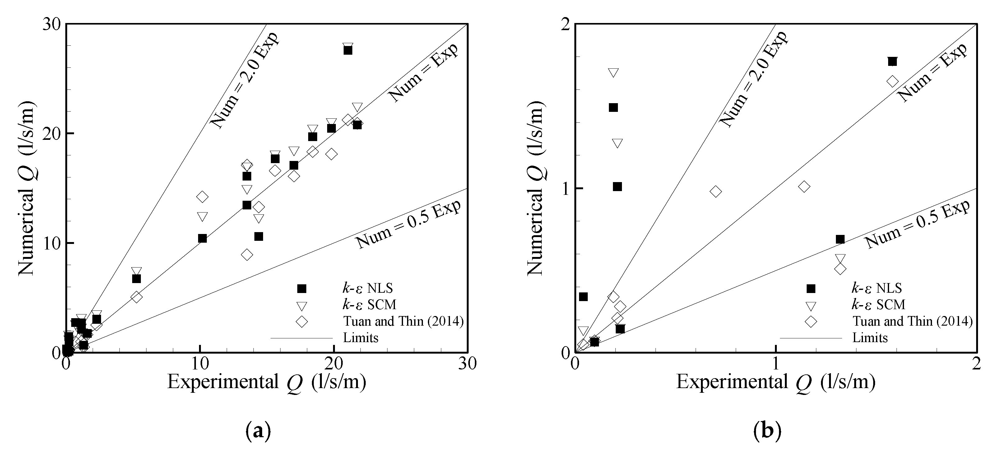
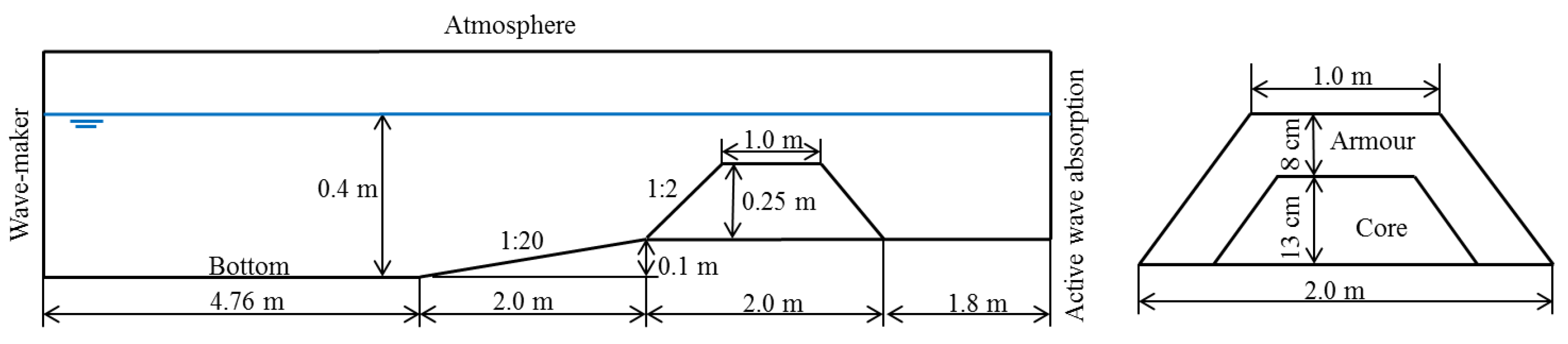
It is very difficult to compare the wave overtopping discharge obtained by numerical models, since it strongly depends on the simulation of phenomena that precede the overtopping, mainly in cases in which the magnitude of the discharge is small. Both wave flume length and wave generation can cause small differences in incident waves which can lead to significant differences on wave overtopping discharge. Nevertheless, the application of FLUENT^® to regular and random waves over impermeable sea dikes with crow-walls showed results of average wave overtopping discharge in good accordance with experimental and numerical ones obtained by Tuan and Thin [18]. NRMSE of average wave overtopping discharges were 38.6 and 34.4% for the k-ε SCM and k-ε NLS turbulence models, respectively, slightly larger than Tuan and Thin [18], which is equal to 23.2%.

(e)

Methodologies developed and implemented in RANS-VoF numerical models to deal with coastal porous structures had good performance, but they are hardly dependent of some empirical parameters that must be set. Regular and random waves over a low-crested rubble breakwater showed good agreement with experimental results, with a NRMSE varying from 5.8 to 15.4% for the k-ε NLS and k-ε SCM turbulence models, respectively, also in agreement with numerical results obtained by Garcia et al. [33]. Regular wave over a rubble mound breakwater presented a slightly larger average wave overtopping discharge than experimental and numerical results obtained by Losada et al. [15].

Although the wave generation and absorption in 3D domains are more complex, all methodologies used for 2D cases in this investigation can also be applied to the more general 3D wave tanks.

References

1. Sakai, T.; Mizutani, T.; Tanaka, H.; Tada, Y. Vortex formation in plunging breakers. In Proceedings of the 20th Conference in Coastal Engineering, Taipei, Taiwan, 9–14 November 1986; pp. 711–723. [Google Scholar]
2. Harlow, F.H.; Welch, J.E. Numerical calculation of time-dependent viscous incompressible flow of fluid with free surface. Phys. Fluids 1965, 8, 2182–2189. [Google Scholar] [CrossRef]
3. Lemos, C.M. Wave breaking: A numerical study. In Lecture Notes in Engineering; Springer: Berlin/Heidelberg, Germany, 1992; Volume 71, pp. 1–185. [Google Scholar]
4. Hirt, C.W.; Nichols, B.D. Volume of fluid VOF method for the dynamics of free boundaries. J. Comput. Phys. 1981, 39, 201–225. [Google Scholar] [CrossRef]
5. Lin, P.Z.; Liu, P.L.F. A numerical study of breaking waves in the surf zone. J. Fluid Mech. 1998, 359, 239–264. [Google Scholar] [CrossRef]
6. Ting, F.C.K.; Kirby, J.T. Observation of undertow and turbulence in a laboratory surf zone. Coast. Eng. 1994, 24, 51–80. [Google Scholar] [CrossRef]
7. Bradford, S.F. Numerical simulation of surf zone dynamics. J. Waterw. Port Coast. Ocean Eng. 2000, 126, 1–13. [Google Scholar] [CrossRef]
8. Mayer, S.; Madsen, P.A. Simulations of breaking waves in the surf zone using a Navier–Stokes solver. In Proceedings of the 25th International Conference in Coastal Engineering, Sydney, Australia, 16–21 July 2000; pp. 928–941. [Google Scholar]
9. Jacobsen, N.G.; Fuhrman, D.R.; Fredsoe, J. A wave generation toolbox for the open-source CFD library: OpenFOAM(R). Int. J. Numer. Methods Fluids 2012, 70, 1073–1088. [Google Scholar] [CrossRef]
10. Brown, S.A.; Greaves, D.M.; Magar, V.; Conley, D.C. Evaluation of turbulence closure models under spilling and plunging breakers in the surf zone. Coast. Eng. 2016, 114, 177–193. [Google Scholar] [CrossRef]
11. Devolver, B.; Trouch, P.; Rauwoens, P. Performance of a buoyancy-modified k-ω and k-ω SST turbulence model for simulating wave breaking under regular waves using OpenFOAM®. Coast. Eng. 2018, 138, 49–65. [Google Scholar] [CrossRef]
12. Chella, M.A.; Bihs, H.; Myrhaug, D.; Muskulus, M. Breaking characteristics and geometric properties of spilling breakers over slopes. Coast. Eng. 2015, 95, 4–19. [Google Scholar] [CrossRef]
13. Chella, M.A.; Bihs, H.; Myrhaug, D.; Muskulus, M. Hydrodynamic characteristics and geometric properties of plunging and spilling breakers over impermeable slopes. Ocean Model. 2016, 103, 53–72. [Google Scholar] [CrossRef]
14. Larsen, B.E.; Fuhrman, D.R. On the over-production on turbulence beneath surface waves in Reynolds-averaged Navier-Stokes models. J. Fluid Mech. 2018, 853, 419–460. [Google Scholar] [CrossRef]
15. Losada, I.J.; Lara, J.L.; Guauche, R.; Gonzales-Ondina, J.M. Numerical analysis of wave overtopping of rubble mound breakwaters. Coast. Eng. 2008, 55, 47–62. [Google Scholar] [CrossRef]
16. EurOtop. Manual on Wave Overtopping of Sea Defences and Related Structures. An Overtopping Manual Largely Based on European Research, but for Worldwide Application. Available online: www.overtopping-manual.com (accessed on 21 September 2021).
17. Soliman, A.; Raslan, M.S.; Reeve, D.E. Numerical simulation of wave overtopping using two dimensional breaking wave model. Trans. Build Environ. 2003, 70, 439–447. [Google Scholar]
18. Tuan, T.Q.; Thin, N.V. Numerical study of wave overtopping on sea-dikes with crown-walls. J. Hydro-Environ. Res. 2014, 8, 367–382. [Google Scholar]
19. Tuan, T.Q.; Oumeraci, H. A numerical model of wave overtopping on seadikes. Coast. Eng. 2010, 57, 757–772. [Google Scholar] [CrossRef]
20. De Finis, S.; Romano, A.; Bellotti, G. Numerical and laboratory analysis of post-overtopping wave impacts on a storm wall for a dike-promenade structure. Coast. Eng. 2020, 155, 103598. [Google Scholar] [CrossRef]
21. Metallinos, A.S.; Klonaris, G.T.; Memos, C.D.; Dimas, A.A. Hydrodynamic conditions in a submerged porous breakwater. Ocean Eng. 2019, 172, 712–725. [Google Scholar] [CrossRef]
22. Dentale, F.; Reale, F.; Leo, A.D.; Carratelli, E.P. A CFD approach to rubble mound breakwater design. Int. J. Nav. Archit. Ocean Eng. 2018, 10, 644–650. [Google Scholar] [CrossRef]
23. Van Gent, M.R.A. Porous flow through rubbe-mound material. J. Waterw. Port Coast. Ocean Eng. 1995, 121, 176–181. [Google Scholar] [CrossRef]
24. Liu, L.-F.; Lin, P.; Sakakiyama, T. Numerical modeling of wave interaction with porous structures. J. Waterw. Port Coast. Ocean Eng. 1999, 125, 322–330. [Google Scholar] [CrossRef]
25. Nakayama, A.; Kuwahara, F. A macroscopic turbulence model for flow in a porous medium. J. Fluids Eng. 1999, 121, 427–433. [Google Scholar] [CrossRef]
26. Getachew, D.; Minkowycz, W.J.; Lage, J.L. A modified form of the k-e model for turbulent flows of an incompressible fluid in porous media. Int. J. Heat Mass Transf. 2000, 43, 909–915. [Google Scholar] [CrossRef]
27. Pedras, M.H.J.; de Lemos, M.J.S. Macroscopic turbulence modelling for incompressible flow through undeformable porous media. Int. J. Heat Mass Transf. 2001, 44, 1081–1093. [Google Scholar] [CrossRef]
28. Hur, D.-S.; Mizutani, N. Numerical estimation of the wave forces acting on a three-dimensional body on submerged breakwater. Coast. Eng. 2003, 47, 329–345. [Google Scholar] [CrossRef]
29. Hur, D.-S.; Lee, K.-H.; Yeom, G.-S. The phase difference effects on 3-D structure of wave pressure acting on a composite breakwater. Ocean Eng. 2008, 35, 1826–1841. [Google Scholar] [CrossRef]
30. Bear, J.; Bachmat, Y. Introduction to Modeling of Transport Phenomena in Porous Media. Theory and Applications of Transport in Porous Media; Kluwer Academic Publishers: Dordrecht, The Netherlands, 1990; Volume 4. [Google Scholar]
31. Whitaker, S. The Method of Volume Averaging. Theory and Applications of Transport in Porous Media; Kluwer Academic Publishers: Dordrecht, The Netherlands, 1999; Volume 13. [Google Scholar]
32. Hsu, T.-J.; Sakakiyama, T.; Liu, P.L.-F. A numerical model for wave motions and turbulence flows in front of a composite breakwater. Coast. Eng. 2002, 46, 25–50. [Google Scholar] [CrossRef]
33. Garcia, N.; Lara, J.; Losada, I. 2-D numerical analysis of near-field flow at low-crested permeable breakwaters. Coast. Eng. 2004, 51, 991–1020. [Google Scholar] [CrossRef]
34. Lara, J.L.; Garcia, N.; Losada, I.J. RANS modeling applied to random wave interaction with submerged permeable structures. Coast. Eng. 2006, 53, 395–417. [Google Scholar] [CrossRef]
35. del Jesus, M.; Lara, J.L.; Losada, I.J. Three-dimensional interaction of waves and porous structures. Part I: Numerical model formulation. Coast. Eng. 2012, 64, 57–72. [Google Scholar] [CrossRef]
36. Jensen, B.; Jacobsen, N.G.; Christensen, E.D. Investigations on the porous media equations and resistance coefficients for coastal structures. Coast. Eng. 2014, 84, 56–72. [Google Scholar] [CrossRef]
37. Higuera, P.; Lara, J.L.; Losada, I.J. Three-dimensional interaction of waves and porous coastal structures using OpenFOAM. Part I: Formulation and validation. Coast. Eng. 2014, 83, 243–258. [Google Scholar] [CrossRef]
38. Vanneste, D.; Troch, P. 2D numerical simulation of large-scale physical model tests of wave interaction with a rubble-mound breakwater. Coast. Eng. 2015, 103, 22–41. [Google Scholar] [CrossRef]
39. Didier, E.; Teixeira, P.R.F.; Neves, M.G. A 3D Numerical Wave Tank for Coastal Engineering Studies. Defect Diffus. Forum 2017, 372, 1–10. [Google Scholar]
40. Teixeira, P.R.F.; Didier, E.; Neves, M.G. A 3D RANS-VOF wave tank for oscillating water column device studies. In Proceedings of the MARINE 2017, Nantes, France, 15–17 May 2017; pp. 710–721. [Google Scholar]
41. Teixeira, P.R.F.; Didier, E. Numerical analysis of the response of an onshore oscillating water column wave energy converter to random waves. Energy 2021, 220, 119719. [Google Scholar] [CrossRef]
42. Shih, T.-H.; Zhu, J. Calculation of wall-bounded complex flows and free shear flows. Int. J. Numer. Methods Fluids 1996, 23, 1133–1144. [Google Scholar] [CrossRef]
43. ANSYS. FLUENT—User’s Guide; ANSYS Inc.: Canonsburg, PA, USA, 2016. [Google Scholar]
44. Wilcox, D.C. Turbulence Modeling for CFD; DCW Industries, Inc.: La Canada, CA, USA, 1993. [Google Scholar]
45. Versteeg, H.K.; Malalasekera, W. An Introduction to Computational Fluid Dynamics: The Finite Volume Method; Pearson Education Limited: London, UK, 2007. [Google Scholar]
46. Harlow, F.H.; Nakayama, P. Transport of Turbulence Energy Decay Rate; University California Report LA-3854; Los Alamos Science Lab: Los Alamos, NM, USA, 1968. [Google Scholar]
47. Menter, F.R. Two-Equation Eddy-Viscosity Turbulence Models for Engineering Applications. AIAA J. 1994, 32, 1598–1605. [Google Scholar] [CrossRef]
48. Ergun, S. Fluid flow through packed columns. Chem. Eng. Prog. 1952, 48, 89–94. [Google Scholar]
49. Engelund, F. On the laminar and turbulent flow of ground water through homogeneous sand. Trans. Dan. Acad. Tech. Sci. 1953, 3, 356–361. [Google Scholar]
50. van Gent, M.R.A. Formulae to Describe Porous Flows. In Communications on Hydraulic and Geotechnical Engineering; Delft University of Technology: Delft, The Netherlands, 1992. [Google Scholar]
51. van Gent, M.R.A. Stationary and Oscillatory Flow through Coarse Porous Media. In Communications on Hydraulic and Geotechnical Engineering; Report No. 1993-09; Faculty of Civil Engineering, Delft University of Technology: Delft, The Netherlands, 1993. [Google Scholar]
52. Santos, G.C.; Teixeira, P.R.F.; Didier, E. Analysis of wave overtopping on an impermeable coastal structure using a RANS-VOF numerical model. In Proceedings of the 25th ABCM International Congress of Mechanical Engineering, COBEM 2019, Uberlândia, MG, Brazil, 20–25 October 2019. [Google Scholar]
53. Neves, M.G.; Didier, E.; Brito, M.; Clavero, M. Numerical and physical modelling of wave overtopping on a smooth impermeable dike with promenade under strong incident waves. J. Mar. Sci. Eng. 2021, 9, 865. [Google Scholar] [CrossRef]
54. Schäffer, H.; Klopman, G. Review of multidirectional active wave absorption methods. J. Waterw. Port Coast. Ocean Eng. 2000, 126, 88–97. [Google Scholar] [CrossRef]
55. Lara, J.L.; Ruju, A.; Losada, I.J. Reynolds averaged Navier-Stokes modelling of longwaves induced by a transient wave group on a beach. Proc. R. Soc. A Math. Phys. Eng. Sci. 2011, 467, 1215–1242. [Google Scholar]
56. Didier, E.; Neves, M.G. A Semi-Infinite Numerical Wave Flume using Smoothed Particle Hydrodynamics. IJOPE 2012, 22, 193–199. [Google Scholar]
57. Higuera, P.; Lara, J.L.; Losada, I.J. Realistic wave generation and active wave absorption for Navier-Stokes models application to OpenFOAM®. Coast. Eng. 2013, 71, 102–118. [Google Scholar] [CrossRef]
58. Fenton, J.D. A fifth-order Stokes Theory for Steady Waves. J. Waterw. Port Coast. Ocean Eng. 1985, 111, 216–234. [Google Scholar] [CrossRef]
59. Fenton, J.D. The numerical solution of steady water waves problems. Comput. Geosci. 1988, 14, 357–368. [Google Scholar] [CrossRef]
60. Barreiro, T.G. Estudo da Interacção de Uma Onda Monocromática Com um Conversor de Energia. Master’s Thesis, Nova University of Lisbon, Nova School of Science and Technology, Costa de Caparica, Portugal, 2009. (In Portuguese). [Google Scholar]
61. Didier, E.; Conde, J.M.P.; Teixeira, P.R.F. Numerical simulation of an oscillation water column wave energy converter with and without damping. In Proceedings of the Fourth International Conference on Computational Methods in Marine Engineering, Lisbon, Portugal, 28–30 September 2011; pp. 206–217. [Google Scholar]
62. Conde, J.M.P.; Teixeira, P.R.F.; Didier, E. Numerical simulation of an oscillating water column wave energy converter: Comparison of two numerical codes. In Proceedings of the 21th International Offshore (Ocean) and Polar Engineering Conference-ISOPE, Maui, HI, USA, 19–24 June 2011; pp. 674–688. [Google Scholar]
63. Teixeira, P.R.F.; Davyt, D.P.; Didier, E.; Ramalhais, R. Numerical simulation of an oscillating water column device using a code based on Navier Stokes equations. Energy 2013, 61, 513–530. [Google Scholar] [CrossRef]
64. Dias, J.; Mendonça, A.; Didier, E.; Neves, M.G.; Conde, J.M.P.; Teixeira, P.R.F. Application of URANS-VOF models in hydrodynamics study of oscillating water column. In Proceedings of the SCACR2015–International Short Course/Conference on Applied Coastal Research, Florence, Italy, 28 September–1 October 2015. [Google Scholar]
65. Mendonça, A.; Dias, J.; Didier, E.; Fortes, C.J.E.M.; Neves, M.G.; Reis, M.T.; Conde, J.M.P.; Poseiro, P.; Teixeira, P.R.F. An integrated tool for modelling OWC-WECs in vertical breakwaters: Preliminary developments. J. Hydro-Environ. Res. 2018, 19, 198–213. [Google Scholar] [CrossRef]
66. Lisboa, R.C.; Teixeira, P.R.F.; Torres, F.R.; Didier, E. Numerical evaluation of the power output of an oscillating water column wave energy converter installed in the Southern Brazilian coast. Energy 2018, 162, 1115–1124. [Google Scholar] [CrossRef]
67. Willmott, C.J.; Ackleson, S.G.; Davis, R.E.; Feddema, J.J.; Klink, K.M.; Legates, D.R.; O’Donnell, J.; Rowe, C.M. Statistics for the evaluation and comparison of models. J. Geophys. Res. 1985, 90, 8995–9005. [Google Scholar] [CrossRef] [Green Version]
Figure 1. Sketch of the computational domain for both wave propagation (a) and wave overtopping cases (b) and the division of the flume by zones of length L for computing ν t / ν .
Jmse 10 01298 g001
Figure 2. Time series of non-dimensional eddy viscosity (spatial average) in zone 1 (a), 4 (b), and 7 (c) for the wave propagation case for the four turbulence models.
Jmse 10 01298 g002
Figure 3. Time series of the free surface elevation in the middle of the wave flume for the wave propagation case for the four turbulence models—dash-lines indicate the mean wave crest and trough obtained by the k-ε NLS model.
Jmse 10 01298 g003
Figure 4. Time series of non-dimensional eddy viscosity (spatial average) in zone 1 (a), 4 (b), and 7 (c) for the wave overtopping case for the four turbulence models.
Jmse 10 01298 g004
Figure 5. Time series of the wave overtopping discharge for the four turbulence models.
Jmse 10 01298 g005
Figure 6. Time series of the wave overtopping discharge for meshes M-1 to M-5.
Jmse 10 01298 g006
Figure 7. Sketch of the computational domain of Ting and Kirby [6] cases. Dimensions in parenthesis represent the plunging case.
Jmse 10 01298 g007
Figure 8. Details of the mesh for the spilling case (Ting and Kirby [6]) near the wave-maker, along the slope and at the end of the domain. The blue line indicates the SWL.
Jmse 10 01298 g008
Figure 9. Maximum and minimum wave height envelopes and mean water level in the spilling case by using k-ε, k-ω SST, k-ε NLS and k-ε SCM turbulence models.
Jmse 10 01298 g009
Figure 10. Maximum and minimum wave height envelopes and mean water level in the plunging case by using the k-ε, k-ω SST, k-ε NLS and k-ε SCM turbulence models.
Jmse 10 01298 g010
Figure 11. Sketch of the computational domain (identical to that of Tuan and Thin [18]).
Jmse 10 01298 g011
Figure 12. Details of the mesh near the wave-maker, along the flume and in the proximity of the dike and vertical wall. The blue line indicates the SWL.
Jmse 10 01298 g012
Figure 13. Numerical (k-ε NLS and k-ε SCM turbulence models and Tuan and Thin [18]) versus experimental (Tuan and Thin [18]) average wave overtopping discharge of regular and random waves: (a) all results and (b) details for small values of wave overtopping discharge.
Jmse 10 01298 g013
Figure 14. Sketch of the computational domain for the porous low-crested rubble-mound breakwater case.
Jmse 10 01298 g014
Figure 15. Details of the mesh near the wave-maker, along the flume (above the ramp) and in the proximity of the low-crested permeable breakwater. The blue line indicates the SWL and the red ones the limits of the porous layers.
Jmse 10 01298 g015
Figure 16. Maximum and minimum wave height envelopes and mean water level of k-ε, k-ε NLS and k-ε SCM models and the experiment (dash line indicates the still water level), T = 1.6 s, H = 0.07 m.
Jmse 10 01298 g016
Figure 17. Maximum and minimum wave height envelopes and mean water level of k-ε, k-ε NLS and k-ε SCM models and the experiment (dash line indicates the still water level), T = 1.6 s, H = 0.10 m.
Jmse 10 01298 g017
Figure 18. Maximum and minimum wave height envelopes and mean water level of k-ε, k-ε NLS and k-ε SCM models and the experiment (dash line indicates the still water level), Tp = 2.4 s, Hs = 0.10 m.
Jmse 10 01298 g018
Figure 19. Maximum and minimum wave height envelopes and mean water level of k-ε, k-ε NLS and k-ε SCM models and the experiment (dash line indicates the still water level), Tp = 3.2 s, Hs = 0.10 m.
Jmse 10 01298 g019
Figure 20. Sketch of the computational domain for the rubble mound breakwater case.
Jmse 10 01298 g020
Figure 21. Details of the mesh near the wave-maker, along the flume and in the proximity of the rubble mound breakwater. The blue line indicates the SWL and the red ones the limits of the porous layers.
Jmse 10 01298 g021
Figure 22. Time series of free surface elevation for k-ε, k-ε NLS and k-ε SCM turbulence models at the gauge x = 42.5 m (near the toe of the breakwater): (a) from 0 to 60 s, and (b) from 240 to 300 s.
Jmse 10 01298 g022
Figure 23. Time series of wave overtopping discharge for k-ε, k-ε NLS and k-ε SCM turbulence models.
Jmse 10 01298 g023