Viscoelastic Wave–Ice Interactions: A Computational Fluid–Solid Dynamic Approach

Abstract

A computational fluid–solid dynamic model is employed to simulate the interaction between water waves and a consolidated ice cover. The model solves the Navier–Stokes equations for the ocean-wave flow around a solid body, and the solid behavior is formalized by the Maxwell viscoelastic model. Model predictions are compared against experimental flume tests of waves interacting with viscoelastic plates. The decay rate and wave dispersion predicted by the model are shown to be in good agreement with experimental results. Furthermore, the model is scaled, by simulating the wave interaction with an actual sea ice cover formed in the ocean. The scaled decay and dispersion results are found to be still valid in full scale. It is shown that the decay rate of waves in a viscoelastic cover is proportional to the quadratic of wave frequency in long waves, whilst biquadrate for short waves. The former is likely to be a viscoelastic effect, and the latter is likely to be related to the energy damping caused by the fluid motion. Overall, the modeling approach and results of the present paper are expected to provide new insights into wave–ice interactions and help researchers to dynamically simulate similar fluid–structure interactions with high fidelity.

1. Introduction

Water waves propagating towards the ice edge are not perfectly reflected, and they can advance in the ice cover. Consequently, waves and ice start to mutually affect each other [1,2]. Waves are weakened as they travel through the sea ice, and the wavelength can be affected by the ice layer. Accurate prediction of the ice-induced energy decay and potential changes in the dispersion process is important for forecasting the wave propagation pattern in ice-covered regions, as well as predicting ice conditions, evolution, and the associated climate impact. In recent years, this topic has been of increasing research interest due to climate change, concerning various processes, e.g., decline of ice extent [3], ice thinning [4], ice shelf vibration and breakup, and Arctic shipping [5,6,7,8].

The interaction between water waves and sea ice in the first place has been studied by using field measurements. Different researchers performed field observations using various techniques to record gravity waves traveling through the sea ice. According to field measurements, wave height was observed to be reduced exponentially, dying out eventually [9,10].

Different mechanisms may trigger the energy damping, depending on the nature of sea ice and fluid motion [11]. Energy damping can be related to the viscous behavior of sea ice [12], the motions of sea ice [13,14], friction [15], turbulent boundary layer formation [16], overwash [17], and the collisions between ice floes [18]. Apart from the energy attenuation, an ice layer can significantly affect the dispersion process of gravity waves, shortening or lengthening the wavelength, compared to an open-water condition. This happens due to changes in the upper layer of the ocean, where the solid cover vibrates, giving rise to vertical motions, causing different types of forces. In the presence of these forces in covered water, the dispersion process is affected, and the wavelengths along with the wave group speed are altered [19]. Clear evidence supporting the effect of sea ice on the wave dispersion process has been documented in some of the recent field observations (see a collection of examples in Collins et al. [20]).

Different theoretical models have been developed to solve the wave–ice interaction to date. They provide us with wave energy decay rates of different sea ice types and enable us to formulate the dispersion relationship (see [21]). The early developed model was constructed by Greenhill back in the 1880s. An elastic layer was assumed to cover the upper layer of an ideal fluid domain. Prescribing a linear motion (i.e., small displacements with no rotation) for solid dynamics, Greenhill [22] formulated the coupled progressive gravity–elastic wave motion and built a dispersion relationship by setting the dynamic pressure of the fluid and solid interface to be equal on the fluid–solid interface. A pure elastic behavior was prescribed for the ice and deformation was assumed to be relatively small, and thus the model was able to construct the dispersion process of a nondissipative ice cover.

The aim of most researchers, in developing wave–ice interaction models, was to either calculate the wave energy decay of sea ice or to include wave scattering in their models, which were lacking in the original work of Greenhill. For example, Hendrickson [23] used an Eigenfunction matching method to solve the wave–ice interaction by prescribing an elastic behavior for the sea ice. The energy damping triggered by the sea ice has been formulated by using different approaches. The nature that is considered for the ice is very important in formulating the energy damping rate of the sea ice. For example, the ice cover can be treated as a viscoelastic thin layer behaving similarly to a Kelvin–Voigt (KV) material [24], or it can be assumed to be a mass of viscous fluid settling down on the water [25]. Additionally, in some other studies, the radiation problem, or the effects of moving loads on ice cover, ice loads on the structures, and impact loads on ice are studied (see examples in [26,27,28,29,30]).

Each of the developed models has been seen to give the energy decay rate or dispersion process with a reasonable level of accuracy over some ranges. That is, although models can accurately predict wave energy decay or dispersion, their boundary of applications is limited. This has been observed in recent years with the increasing growth in flume/basin and field experiments. For example, a model that was presented by Fox and Squire [31] was later further extended by adopting a viscoelastic behavior for the ice layer by Moisg et al. [32]. This model is able to capture the wave energy decay over shorter wavelengths, but its results diverge from experimental field data as the wavelength increases (see landfast tests of Voermans et al. [33]), or the model has been seen to fail in reconstructing the energy decay rate curves of a viscoelastic body interacting with regular waves, but it was found to fairly predict the dispersion process under that cover (see Sree et al. [34]). The main reason is perhaps the assumptions made for the ice cover as the sea ice mechanics is related to a complex field of research. Different types of ice can be formed on the water surface and the environment in which the ice forms and ice aging can affect the ice behavior. This leaves us with a wide range of options in building wave–ice interaction models. Yet, theoretical models normally assume fluid is irrotational, by which viscous, turbulent, and nonlinear fluid behaviors are excluded.

The fluid can be assumed to be viscous. This may enable us to reproduce the wave–ice interaction with less restriction (i.e., viscous fluid-based energy damping and nonlinearities can be considered). Navier–Stokes (NS) equations govern fluid motion, which cannot be solved analytically except for some limited problems. Instead, computational methods, such as the meshed ones or meshfree ones, are used to solve the NS equations. We need to keep in mind that the wave propagation of irrotational flow may need numerical methods as well (e.g., [35,36,37]).

To simulate the interaction of viscous fluid with an ice layer, the fluid dynamics problems are coupled with the solid dynamic problems. The solid body can be assumed to be rigid or flexible. The rigid body assumption may provide us with energy damping caused by the fluid motion (e.g., Bai et al. [38], Tavakoli and Babanin [39]), whereas a flexible body assumption empowers us in the prediction of dispersion process and solid-based energy damping—the former is possible if the solid body is assumed to be viscoelastic. The solution of the interaction between the solid body and the viscous fluid can be achieved using one-way and two-way coupling. The former is recommended to be used when the solid motion is not significant [40], because the solid effects on the fluid field are inconspicuous, but the two-way coupling is preferred over the one-way coupling when the solid motion can remarkably affect the fluid motion. When ice interacts with water waves, the second scenario is more possible, and a two-way coupling approach needs to be considered to carry out a more realistic simulation.

The two-way coupling of the viscous fluid and solid motions can be achieved by matching solid and fluid dynamics solvers. This has usually been carried out by coupling finite volume method (FVM) solvers of fluid motion and finite element method (FEM) solvers of solid motion which solve beam/plate theories. Examples can be found in the research concerned with the elastic motions of ships and marine structures exposed to water waves and sea loads (e.g., Jiao et al. [41], Sun et al. [42], Lakshmynarayanana and Hirdaris [43], Hosseinzadeh and Tabri [44]).

The FVM has also been used for the simulation of the solid motions in fluid–solid interaction (FSI) problems. Instead of using beam or plate theories, the momentum conservation of the displacement rate in the solid domain is solved, and the momentum balance is prescribed on the fluid–solid boundaries. Huang et al. [45] and Huang and Li [46] have used this method for reproducing the interaction of water waves with elastic ice sheets, and elastic breakwaters, respectively. Through their simulations, the method was observed to be accurate. Simulations performed by Huang et al. [45] addressed the elastic motions and considered the fluid-based energy attention caused by the ice plate (i.e., partial reflection and overwash). However, Huang et al. [45] did not consider viscoelastic solid bodies. To better represent wave–ice interactions, the ice can be solved as viscoelastic bodies, because ice in waves tends to present viscoelastic behavior rather than elastic (Sree et al. [34]). Thus, enabling viscoelastic modeling of sea ice will enhance understanding and prediction of wave–ice interactions, which is lacking at the moment. It should be noted that the computational models may need a very long time to be run, and they cannot be directly implemented in global wave modeling. Additionally, artificial effects may emerge due to numerical techniques, giving larger energy dissipation. Moreover, when a computational model under a viscous flow assumption is used, it is very hard to single out the effects of one parameter in the whole fluid–solid dynamic problem, as the simulations is performed using a nonlinear approach and effects of all physical phenomena are acquired at once (e.g., when the wave–plate interaction is run, the fluid motion caused by radiation and diffraction cannot be achieved separately). However, as computational models built on the basis of the viscous flow assumptions are less restricted than the potential flow theory, their results may provide a deeper understanding of the problem.

In the present paper, a computational fully coupled FSI model is used to solve the interaction of water waves with a viscoelastic ice sheet. This model solves the air–water flow around an integrated viscoelastic floating body with a finite length. An initial aim of this research is to evaluate whether the presented model can be used to numerically reconstruct wave–ice interaction problems. Thus, the model is first validated by comparing the obtained results against experimental data collected in flume measurements. Upon the experimental validation, the scalability of the model is studied to find whether a full-scale sea ice cover can be scaled into a small-scale floating body. For this purpose, field tests of full-scale sea ice are reproduced through a scaling approach, and the accuracy level in predicting the energy decay rate and dispersion process is evaluated.

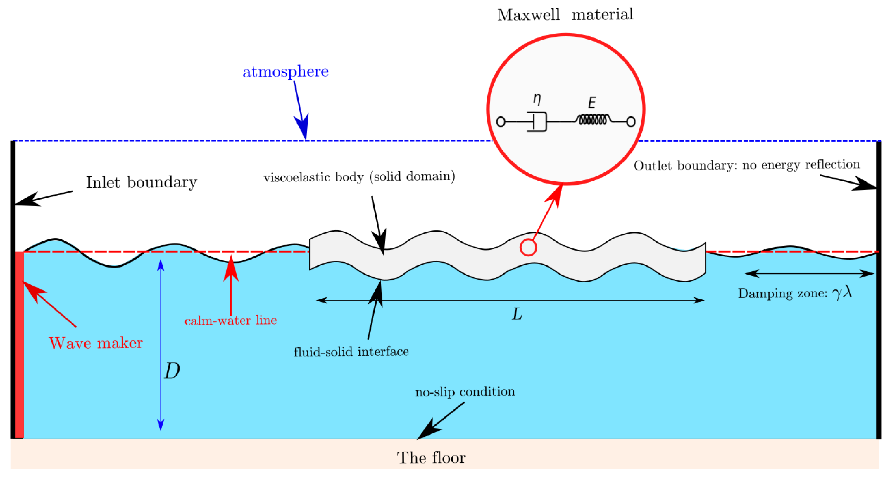
2. Problem Statement

2.1. Overall Description of the Problem

An integrated ice layer covering water with a finite depth of $D$ is considered, as shown in Figure 1. Assuming that a monochromatic wave with a height of $H_0$ at a point with a longitudinal location of $x_0$ travels into the cover, its wave height is decayed exponentially, as per

$$H\left(x\right)=H_0 e^{-{\alpha }_i\left(\mathrm{x}-x_0\right)}.$$

(1)

Here, ${\alpha }_i$ is the amplitude decay rate which is sensitive to the fluid properties and the mechanical behavior of the ice covering the liquid. Water waves are assumed to be harmonic and regular. This allows us to formulate the vertical motion of the free surface in an open-sea condition, as

$$\xi \left(x,t\right)=H/2 cos\left(k_{o}x-\omega t\right).$$

(2)

In Equation (2), $\omega =2\pi ⁄T$ is the frequency and $k_o=2\pi ⁄{\lambda }_o$ is the wavenumber of the open-sea condition, which are linked together through

$${\omega }^2=gk \tanh kD.$$

(3)

In Equation (3), $g$ is the gravity acceleration constant and equals 9.81 m/s².

When the interaction between water waves and a viscoelastic cover is studied, one of the main challenges is to find the value of ${\alpha }_i$ and the potential changes in the wavelength. In the next sub-section, the theoretical background, and formulations, which can be employed to calculate these two parameters, are explained.

2.2. Theoretical Background

The mutual interaction between water waves with a viscoelastic ice cover can be formulated by using fundamental theories. It is assumed that a thin layer of viscoelastic body covers the upper layer of water. This layer has a thickness of $h$. The domain is assumed to have a finite depth of $D$, and the extent of the cover is hypothesized to span over an infinite length. Water fluid is assumed to be ideal, and thus the potential field represents the fluid motion in the domain. Hence, the fluid motion obeys the Laplace equation. The solid motion of the cover is hypothesized to be very small. Thus, it follows the Euler–Bernoulli beam theory. The cover is supposed to be viscoelastic, as mentioned. Accordingly, stress and strains can be linked through a viscoelastic model. A Kelvin–Voigt model is assumed to link up the stress ($\sigma$), strain (ε), and strain rate ($\dot{\epsilon }$), as

$$\sigma =G\epsilon +\eta \dot{\epsilon }.$$

(4)

Here, $G$ is the shear modulus of the material and $\eta$ is the dynamic viscosity of it.

By assuming that solid displacements of the ice layer obey the Euler–Bernoulli beam theory, a kinematic boundary condition for the upper layer of the water can be formulated. Then, the dispersion can be built by assuming a harmonic motion for the fluid, as per

$${\omega }^2=\left(\frac{G{h}^3}{6{\rho }_w}{k}^4-i\omega {\rho }_i\eta \frac{h^3}{6{\rho }_w}{k}^4-\frac{{\rho }_i}{{\rho }_w}{\omega }^2-g\right)k \tanh kD.$$

(5)

In a deep-water condition, the above equation has five roots for $k$, four of which are complex numbers. The dominant root, related to progressive wave, is written as

$$k=k_i-i{\alpha }_i.$$

(6)

Here, $k_i$ (the real part) is the wavenumber related to waves propagating in the ice-covered sea and ${\alpha }_i$ (the imaginary part) is the wave height decay rate, which was previously introduced in Equation (1). Note the above method was originally formulated by Fox and Squire [31] but was adopted for KV material by Moisg et al. [32]. Discussions on the roots of the dispersion equation are presented in Fox and Squire [31].

2.3. Scaling Law

To study the role of a viscoelastic cover on wavenumber and wave amplitude of waves traveling from uncovered sea to covered sea, dimensionless parameters are identified. To do so, Buckingham Pi-theorem is employed. Parameters that are involved in the problem are the wavelength in open-sea (${\lambda }_o$) condition, wavelength under the viscoelastic cover (${\lambda }_i$), amplitude decay rate (${\alpha }_i$), Young’s modulus of the cover ($E$), ice viscosity ($\eta$), the thickness of cover ($h$), water density (${\rho }_w$), the density of the cover (${\rho }_i$) and the gravity acceleration ($g$). Three main physical parameters, mass, time, and length, are incorporated. Accordingly, five dimensionless numbers should be formulated. The following dimensionless numbers are identified:

The first dimensionless number is normalized wavelength in open water, which can be formulated as

$${\widehat{\lambda }}_o={\lambda }_o/h.$$

(7)

This number represents the ratio of the wavelength over the thickness of the cover.

The second dimensionless number is

$${\widehat{k}}_i=k_i/k_o={\lambda }_o/{\lambda }_i.$$

(8)

This number describes the relative wavenumber under the ice cover (see, e.g., in [34]). The third dimensionless number is formulated as

$${\widehat{\alpha }}_i={\alpha }_i/k_o.$$

(9)

${\widehat{\alpha }}_i$ indicates the normalized decay rate. The fourth dimensionless number is

$$\widehat{E}=\surd \left(E/{\rho }_i\right)/\surd \left(gh\right),$$

(10)

which describes the elasticity per unit mass (see [47]). The other dimensionless number is

$$\widehat{\eta }=\eta /{\rho }_i \surd \left(g{h}^3\right).$$

(11)

The above number indicates the viscosity per mass of the material. The last dimensionless number is

$${\widehat{\rho }}_i=\frac{{\rho }_i}{{\rho }_w},$$

(12)

which is the relative density of the ice. The normalized dispersion equation of a deep-water condition, i.e., $\tanh kD\sim 1$, is built as

$$\frac{\widehat{E}\widehat{\rho }{\left(2\pi \right)}^3}{12\left(1-\nu \right){{\widehat{\lambda }}_o}^4}{\widehat{k}}^5-i\frac{\widehat{\eta }\widehat{\rho }{\left(2\pi \right)}^3}{6\left(1-\nu \right){{\widehat{\lambda }}_o}^4}{\widehat{k}}^5-\widehat{k}-\frac{\widehat{\rho }}{{\widehat{\lambda }}_o}\widehat{k}-1=0.$$

(13)

$$A=\frac{\widehat{E}\widehat{\rho }{\left(2\pi \right)}^3}{12\left(1-\nu \right){{\widehat{\lambda }}_o}^4},B=\frac{\widehat{\eta }\widehat{\rho }{\left(2\pi \right)}^3}{6\left(1-\nu \right){{\widehat{\lambda }}_o}^4},C=\frac{\widehat{\rho }}{{\widehat{\lambda }}_o}.$$

Thus, there are three dimensionless parameters $A, B,$and $C$ which determine the dispersion relation. Note that ${\widehat{\lambda }}_o$ is related to wave frequency through an open-water dispersion relationship. The root of the above equation gives the relative wavenumber. When we present dispersion curves, we plot wavenumber versus wave frequency. For this aim, we plot $kh$ versus dimensionless frequency which is a product of $\omega$ and $\sqrt{h/g}$.

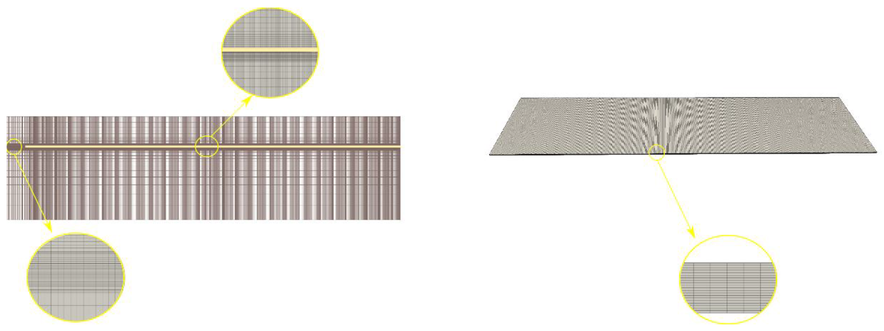
3. Computational Model

3.1. Problem Formulation

A two-dimensional fluid domain that is bounded at its two ends at the left and right is considered. This fluid domain is filled with two phases: air and water. The water depth is $D$. In this domain, a floating viscoelastic solid body is located that can mutually interact with water waves. Fluid is also assumed to be incompressible.

We define three unknown parameters for the fluid flow. The first one is the fluid velocity at any point in the domain, which is shown by $\mathit{v}=\mathit{v}\left(\mathit{x};t\right)$. The next one is the pressure $p=p\left(\mathit{x};t\right)$, which is equal to the atmospheric pressure above the water surface and varies linearly by the increase in the depth under the water when there is no fluid motion. As the fluid particles move from one point to another, pressure changes due to the changes in the momentum. The last unknown parameter is the volume fraction, $ℱ=ℱ\left(\mathit{x};t\right)$, which denotes the volume fraction field.

We use an Eulerian approach to formulate the equations governing the velocity and pressure fields. The fluid is assumed to be Newtonian. As such, the shear stresses, generated near the walls and the boundaries, change linearly with the increase in the velocity gradient.

Considering a two-phase fluid domain, two equations govern the velocity and pressure fields in the domain. The first one is the continuity equation of an incompressible fluid flow, which is given by

$$\nabla ·\mathit{v}=0.$$

(14)

The next equation is the momentum equation, which was formulated by Navier and Stokes, connecting velocity and pressure fields of Newtonian flow. The Navier–Stokes equation is given by

$${\rho }_{\mathrm{m}}\left(\frac{D\mathit{v}}{Dt}\right)=-\nabla p+{\mu }_m{\nabla }^2\mathit{v}+\frac{1}{3}{\mu }_m\nabla \left(\nabla ·\mathit{v}\right)+{\rho }_m\mathit{g},$$

(15)

where ${\rho }_m$ and ${\mu }_m$ denote the effective values of the fluid (density and dynamic viscosity). The values of these two parameters vary at different points of the two-phase fluid domain depending on the volume fraction of each phase, $\mathit{g}$ is the gravity vector.

The volume fraction field ($ℱ$) is applied to model the air–water flow and obeys the following equation:

$$\frac{\partial ℱ}{\partial t}+\mathit{v}·\nabla ℱ=0.$$

(16)

The properties of the air–water mixture are computed by

$${\rho }_m=\left(1-ℱ\right){\rho }_a+ℱ{\rho }_w,$$

(17)

$${\mu }_m=\left(1-ℱ\right){\mu }_a+ℱ{\mu }_w.$$

The left and right ends of the domain are respectively equipped with a numerical wavemaker and a numerical wave damper. The numerical wavemaker generates linear water waves with the frequency of ω. The velocity profile of the fluid motion generated by the surface waves obeys a linear theory as

$$\{\begin{array}{c}{v}_x\left(\mathit{x},t\right)=\frac{H}{2}\omega e^{kz}\cos \left(kx-\omega t\right),\\ v_z\left(\mathit{x},t\right)=\frac{H}{2}\omega e^{kz}\sin \left(kx-\omega t\right).\end{array}$$

(18)

On the floor of the fluid domain, an impermeable sea-bed is considered. No-slip condition is satisfied on this surface, and thus shear stresses may emerge. The upper surface of the domain is an open atmosphere boundary (see Figure 2).

The viscoelastic body is identified as the solid domain. We present the equations governing this domain by using a conservative-based approach. The length and thickness of the solid body are$L$ and $h$, respectively. Assuming that motions in the solid body are small, we can neglect the difference between the deformed and undeformed configurations. We define the relative displacement in the solid by the vector $\mathit{u}\left(\mathit{x};t\right)$. The motions obey a conservation equation, given by

$${\displaystyle \int }{\rho }_B\frac{{\partial }^2\mathit{u}}{\partial t^2}d{\mathit{\Omega }}_{\mathit{S}}={{\displaystyle \oint }}_{{\mathit{\Gamma }}_{\mathit{S}}}\mathit{n} · \mathit{\sigma } d{\mathit{\Gamma }}_{\mathit{S}}+{{\displaystyle \int }}_{{\mathit{\Omega }}_{\mathit{S}}}{\rho }_B\mathit{b}d{\mathit{\Omega }}_{\mathit{S}}.$$

(19)

Here, ${\mathit{\Omega }}_S$ is the solid domain, and ${\mathit{\Gamma }}_S$ indicates the surfaces of the solid. $\mathit{b}$ is the body force vector, $\mathit{\sigma }$ is the stress tensor which is related to the strain tensor ($\mathit{e}$) by the general Maxwell equation, as

$$\mathit{\sigma }\left(t\right)={{\displaystyle \int }}_{-\infty }^{t}g\left(t-s\right)2\mu \mathit{e}ds+\kappa \mathrm{Tr}\left[\mathsf{ϵ}\right]I g\left(t\right)={\gamma }_{\infty }+{{\displaystyle \sum }}_{i=1}^N{\gamma }_i\exp \left(-t/{\tau }_i\right).$$

(20)

In the above equation, ${\gamma }_{\infty }$ is the Young’s modulus of the elastic element, and ${\gamma }_i$ is the Young’s modulus of the i-th element of the model. In addition, $\mathrm{Tr}$ is the trace operator. ${\tau }_i$ is the relaxation time of the i-th element, and is found as

$${\tau }_i={\eta }_i/{\gamma }_i,$$

(21)

where ${\eta }_i$ is the viscosity of the i-th element. $\mathit{e}$ is the deviatoric component of the strain tensor, which is given by

$$\mathit{e}=\mathrm{dev}\left(\mathsf{ϵ}\right)=\mathsf{ϵ}-1/3\mathrm{tr}\left[\mathsf{ϵ}\right]I.$$

(22)

Here, $\mathit{I}$ is the unit matrix and $\mathsf{ϵ}$ is the strain tensor, which is calculated as

$$\mathsf{ϵ}=\mathrm{symm}\left[\nabla \mathit{u}\right]=\frac{1}{2}\left(\nabla \mathit{u}+\nabla {\mathit{u}}^T\right).$$

(23)

All surfaces of the solid are surrounded by fluid (either air or water). Conditions of a fluid–solid coupling boundary are therefore satisfied on these surfaces. This means that, first, kinematic boundary conditions govern the motion of the fluid–solid structure, i.e., velocity, and displacements of the solid and fluid particles are equal on the fluid–solid surfaces:

$${\mathit{u}}_F={\mathit{u}}_S,$$

(24)

$${\mathit{v}}_F={\mathit{v}}_S.$$

In addition, dynamic boundary conditions are also satisfied on the fluid–solid boundary as

$$\mathit{n}·{\mathit{\sigma }}_F=\mathit{n}·{\mathit{\sigma }}_S,$$

(25)

where n is the normal vector. ${\mathit{\sigma }}_F$ and ${\mathit{\sigma }}_S$, respectively, refer to the fluid and solid stress tensor.

The stress tensor generated by the fluid motion (${\mathit{\sigma }}_F$) is computed by

$$\mathit{n}·{\mathit{\sigma }}_F=-pI+\mathit{\tau },$$

(26)

where τ is the shear stress tensor and $p$ is the fluid pressure. The traction at the fluid–solid interface is related to the velocity of solid as

$$\mathit{n}·{\mathit{\sigma }}_S=-p{\mathit{n}}_i+\mu {\mathit{n}}_i·\nabla {\mathit{v}}_t-2{\mu }_m\left({\nabla }_s·{\mathit{v}}_s\right){\mathit{n}}_i+{\mu }_m{\nabla }_s{\mathit{v}}_s.$$

(27)

Here, ${\nabla }_s=\nabla -\mathit{n}\mathit{n}·\nabla ,$ which is the surface tangential gradient operator.

3.2. Computational Technique

The problem is solved by using OpenFOAM code, which allows us to decompose the equations governing the fluid and solid domains by using the finite volume method (FVM). The solids4Foam library is used [48], by employing which the coupled fluid–structure interaction problem can be simulated numerically. The upstream length is set to be greater than $3{\lambda }_o$ and the downstream length is set to be greater than $6{\lambda }_o$ in all tests. This prevents any artificial effect that the body can have on the wave generation.

The transient terms of both solid and fluid motions are decomposed by using an implicit method. Convection terms are decomposed by using a second-order method. Diffusion terms are decomposed by applying a second-order method. The Gauss linear method is used for the numerical solution of the unknown matrices. The tolerance values of the pressure and velocity are respectively set to be ${10}^{-8}$ and ${10}^{-6}$. The fluid problem is solved by using the interFoam solver. The pressure correction method is performed with a tolerance of $0.001$. The momentum equations are solved by applying a Pressure-Implicit with Splitting of Operators (PISO) algorithm. Water waves are generated by using the waves2foam library [49,50]. Waves are generated at the left boundary. A relaxation zone as long as ${\lambda }_o$ is defined forward the wave-maker. This allows water waves to be developed over a wavelength distance and decreases numerical errors. Waves are dampened near the right end of the domain, where a damping zone is generated. Thus, no wave reflection occurs. The damping zone spans over a length of $\mathsf{\gamma }{\lambda }_o$, where $\mathsf{\gamma }$ is set to be equal to 2. The Courant number is set to be lower than 0.5 at all time steps. This stops the growth of errors over time and simulations may not diverge.

The water surface is initialized to be calm, and then water waves are generated. A ramp time is set to avoid any sudden change in the water surface elevation. This ramp time is set to be two times greater than the wave period. Simulations are run up to 17 wave periods, which ensures that 15 cycles of desirable regular waves were simulated to capture valid data. Data are sampled with a frequency of $1000 \mathrm{Hz}$. Readers interested in simulating wave-structure interaction using OpenFOAM are referred to [51].

A structured mesh strategy is used as shown in Figure 3. Orthogonal cells are generated as the geometries of both fluid and solid domains are very simple. Cells are set to have finer size near the free surface, and in the vicinity of the cover. In the free surface neighborhood, the ratio of the length of the cell over its height has a maximum value of 1.5, which cancels out the artificial numerical energy damping that can be triggered by the cell size. A mesh study is also performed to evaluate the effect of cell size on the generated waves, and to find the cell size that can be employed to simulate the problem. The results of the mesh study are presented in Appendix A. In the solid domain, cells are set to be structured as well. The longitudinal motion of the solid body is stopped by defining vertical virtual patches, on which the shear stress is set to be zero. This means that, while these patches transport the momentum, they never have any longitudinal motion. The mesh motion is performed by computing the velocity of the fluid–solid interface. The mesh is regenerated at every single time step. A tolerance of ${10}^{-6}$ is set for the cell motions.

4. Studied Cases

Three different sets of experiments are studied in the present research. Related experiments took place in flume and in an actual Arctic field. The first set of flume tests were carried out by Sree et al. [52], who documented the wave interaction with viscoelastic covers. The second set of flume tests were carried out by Yiew et al. [53], who measured dispersion and dissipation of gravity waves traveling through a continuous ice sheet. The Arctic field tests were carried out by Voermans et al. [33], who measured wave dispersion and dissipation in landfast ice. The first set of experiments helps us to evaluate the validity of the model. The second and third sets of experiments help us to find the viscosity of ice and evaluate the ability of the model in simulating wave–ice interaction. Meanwhile, a scale effect study is also performed to examine whether the present computational fluid–solid model follows the scaling law or not.

5. Results and Discussion

5.1. Viscoelastic Cover Exposed to Water Waves

The first set of tests are performed to model interactions of four different solid covers with water waves, aiming to evaluate the accuracy of the method in the reconstruction of wave interaction with a viscoelastic sheet. Tests were performed by Sree et al. [52]. Decay rates and the dispersion process were measured. Through dry dynamic tests, the solid material was observed to follow the KV model. The summary of the measured storage and loss moduli is presented in Figure 4.

In the present research, as stated before, a Maxwell model is used to calculate the shear stress generation in the solid cover. The storage and loss moduli of a Kelvin–Voigt material are given as

$$G^{\prime }=G,$$

(28)

$$G^{″}=i\omega \eta .$$

(29)

In addition, the storage and loss moduli of Maxwell material are formulated as

$$G^{\prime }=\frac{G\left({\tau }^2{\omega }^2\right)}{\left(1+{\tau }^2{\omega }^2\right)},$$

(30)

$$G^{″}=i\frac{G\left(\tau \omega \right)}{\left(1+{\tau }^2{\omega }^2\right)}.$$

(31)

To run the model, the storage and loss moduli are kept constant, and the relaxation time and the shear modulus are calculated. Here, it should be noted that it is more reasonable to assume that the loss moduli are linear functions of frequency, as seen in Figure 4. However, as the present computational approach embedded in OpenFOAM does not include the Kelvin–Voigt model, we have used the Maxwell model.

5.1.1. Viscoelastic Cover Exposed to Water Waves

In this sub-section, the results corresponding to the wave interaction with viscoelastic covers considered in the present research are presented. Simulations are run for four different covers with different material properties. The main aim is to evaluate the accuracy of the computational fluid–solid model and the setup in numerical replication of the problem. In one case, the left end of the cover is set to be fixed. Such a scenario resembles the interaction of water waves with a cantilever beam. In the experiments performed in the wave flume, the left end was set to be free. The cantilever simulation is run to evaluate whether the fixed end can affect the results or not.

Samples of the recorded wave at two different points on the cover, located with a distance of 0.2 m from each other, are shown in Figure 5. The presented curves are the time series of the deformation of the cover.

As seen, there is a time lag between the recorded wave motions at these two points, signifying that the wave celerity can be calculated by using the time differences between similar phases. This was carried out later.

It can also be seen that the amplitude of the blue curve is slightly smaller than that of the red curve. This confirms that waves are reduced as they propagate into the viscoelastic cover. This well matches with the physics of the problem since the cover is viscoelastic, and is expected to dampen the energy of the fluid motion.

5.1.2. Example of Wave Attenuation

The wave height at any point of the cover can be calculated. This has been carried out by using a zero-crossing approach. Wave heights of fifteen cycles are computed and then the average value is calculated. Examples of the recorded wave heights along the viscoelastic cover are shown in Figure 6. One of the examples corresponds to a cover clamped at its right end, and the other shows the wave height variation of a viscoelastic cover having two free ends. Presented results in this figure are related to waves with an open-water wavelength of 72 h (wave period of $0.75$ s). Two solid curves demonstrate the computed wave heights. The dashed curves show the exponential curves fitted through the numerical data.

The cover with one fixed end is seen to lead to a lower damping rate, compared with the cover having two free ends. The possible reason for this behavior is the elastic wave motion reflected by the clamped end, which can result in a partial standing wave in the cover. The damping ratio of the free–free cover is closer to that of the experimental value, measured by Sree et al. [52].

5.1.3. Example of Wave Attenuation

As was seen in Figure 5, there is a phase lag between the recorded waves at two different points. Hence, the phase speed of waves traveling into the cover can be computed. Consequently, the wavelength and wavenumber can be calculated.

The phase lag between two points, located with a distance of $\delta x=12.5 \mathrm{h}$ (corresponding to $0.125 \mathrm{m}$) from each other, is computed. The phase speed is calculated by using

$$c_i=\frac{\delta x}{\delta t}.$$

(32)

Here, $\delta t$ is the time lag between two consecutive wave crests. Then, the wavelength is computed by

$${\lambda }_i=c_{i}T.$$

(33)

By using the computed wavelength, the wavenumber under the viscoelastic body is computed by

$$k_i=2\pi /{\lambda }_i.$$

(34)

Wavenumber under the viscoelastic cover is computed over fifteen cycles at different points. Then, the mean value of the phase speed recorded at every point is found, which is compared against experimental data in one of the upcoming sub-sections. Figure 7 shows examples of the recorded phase speed along the viscoelastic cover. This figure includes four different panels, each of which demonstrates the results corresponding to a different wave period. In all panels, the phase speed is normalized by using phase speed of the open-sea condition, which helps us interpret the data more easily. As is apparent, phase speed does not have a constant value along the cover. It varies locally, though the variation is not very significant. It can be concluded that the phase speed is practically constant along the cover and the variations are likely to be caused by the artificial effects. The phase speed of the shortest wave is seen to be greater than 1.0, signifying that the developed wave becomes longer under the cover.

5.1.4. Snapshots

Snapshots of the simulations are shown in Figure 8, providing us with an image of the water surface profile around the viscoelastic cover interacting with water waves. Four different panels are shown in this figure. Each of these panels corresponds to the water field around the cover at a specific instant. The time interval between the snapshots is $0.25 \mathrm{T}$. This covers a full wave period. Water is marked with yellow and the cover is marked with red. As seen, the wave crest in the front field, left, is in a different location at each instant. In addition, the transmitted wave field, right, is seen to be lower compared to the waves observed in the left. This demonstrates that wave height reduces under the effects of the viscoelastic cover, which matches with the physics.

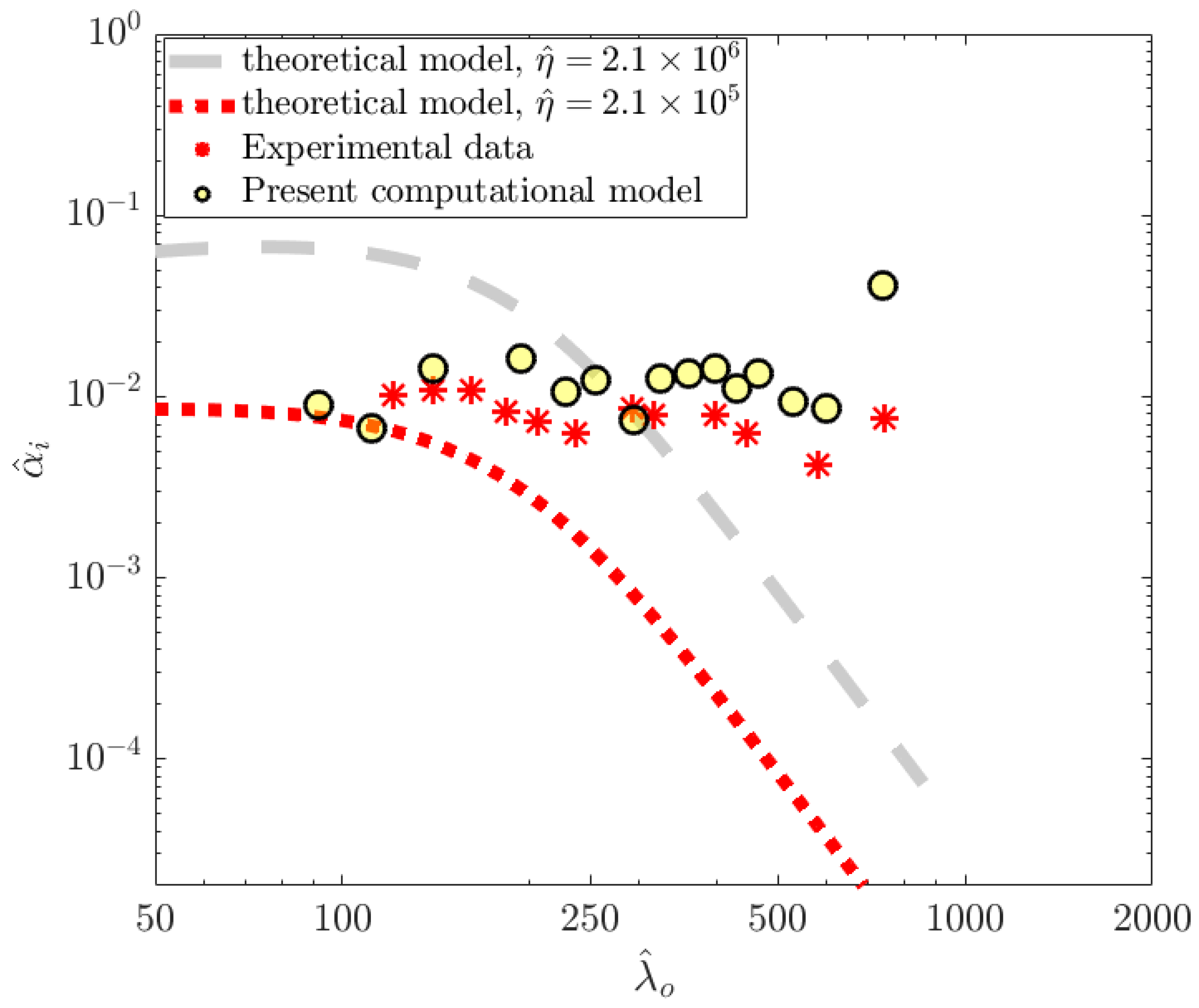
5.2. Validation of the Model

The present computational fluid–solid model is validated by comparing its results against the experimental work of Sree et al. [52], as explained previously. Sree et al. [52] documented the decay rates and wavenumbers of covers interacting with water waves over a wide range of wavelengths.

Figure 9 shows the normalized attenuation rates as a function of normalized wavelength in an open-sea condition. Note that the cover has a finite length, and it is reasonable to plot decay rate as a function of wavelength of the open-water condition (as in seakeeping analysis). Note that the decay rate versus frequency plots shall be presented in Section 5.6.

Four different panels are shown in Figure 9. Each panel displays the data corresponding to a specific cover. The mechanical properties of these covers have been described earlier in Figure 4. In addition, the values that the theoretical model gives are also plotted in this figure. As seen, ${\widehat{\alpha }}_i$ might change and decrease with an increase in ${\lambda }_o$ over the tested wave condition. Experimental data and the ones that are predicted by the computational fluid–solid model are seen to be close to each other in most cases. The attenuation rates of cover 1 and cover 2 are seen to be slightly over-predicted by the present model. These two covers have lower rigidity. Hence, larger stresses may emerge in the body when it flexes. Thus, larger errors are more likely to occur. Attenuation rates of cover 3 and cover 4, however, are computed with a greater level of accuracy. The theoretical model is seen to under-predict the attenuation rates significantly. The attenuation rate that the theoretical model gives monotonically reduces with the increase in open-water wavelength. The theoretical model is formulated by considering viscoelastic behavior for the material. However, other mechanisms, such as water damping, or added mass variation over the length of the cover, may contribute to energy dissipation. The contribution of these mechanisms to energy dissipation is more likely to be great in small frequencies. Inasmuch as the present computational FSI model considers fluid motion around the body without restricting the fluid motion-induced damping, it can capture the effects of the mentioned mechanisms. Thus, its data are much closer to experimental data compared to the ones predicted by the theoretical model.

Figure 10 shows a comparison between dispersion curves found through experiments and those of the present model. The horizontal axis refers to the dimensionless wave frequency and the vertical axis shows the product of wavenumber and thickness of the cover. The curves constructed by the theoretical model are also plotted. The open-water dispersion curve is also added to the figure.

The wavelength in the covered water is longer than that of the open-water condition when open-water waves are short, i.e., wavenumber in the covered region is smaller than that of the uncovered region. This has been seen to occur when waves interact with covers 3 and 4. However, cover 1 and cover 2 do not increase the wavelength of generated waves (the markers are not below the red curve). The reason for this behavior is that covers 3 and 4 have larger Young’s moduli, and thus they can increase the wavelength more significantly.

When a progressive wave has a shorter frequency, the viscoelastic cover may make them shorter, compared to open-sea conditions (markers can be above the red curve). However, note that this change, the decrease in the wavelength (increase in the wavenumber), is not significant. The lengths of waves obtain 95% of their initial value for covers 1 and 2. Interestingly, the cover with a larger stiffness value, which has larger shear modules, makes waves longer at a wider range of wave frequency. This shows that the stiffness of the cover has a very important role in the dispersion relationship. The results of the computational fluid–solid model and experiments are seen to be in fair agreement. There are some differences, which might be due to numerical errors of the model, possible wave reflection from the free end or even the sampling frequency used for recording the data.

The theoretical model works with a great level of accuracy. As discussed previously, the theoretical model under-predicts the attenuation rate. Here, a very important message can be taken. When the dispersion and attenuation rate of a viscoelastic cover with a finite length are calculated by using a theoretical model, the attenuation coefficient may be computed with a large error, but the dispersion of waves is computed with a great level of accuracy. Note that some experiments have proven that the presence of notches or cracks also affects the accuracy of the theoretical model. However, for the present viscoelastic cover, the mass of the body is homogeneous, and there is no sudden change in vertical displacement and stresses. Any crack or sudden change in the body can affect the physics of the problem and, of course, can decrease the effects of stiffness/rigidity of the cover (Squire and Dixon [54,55]).

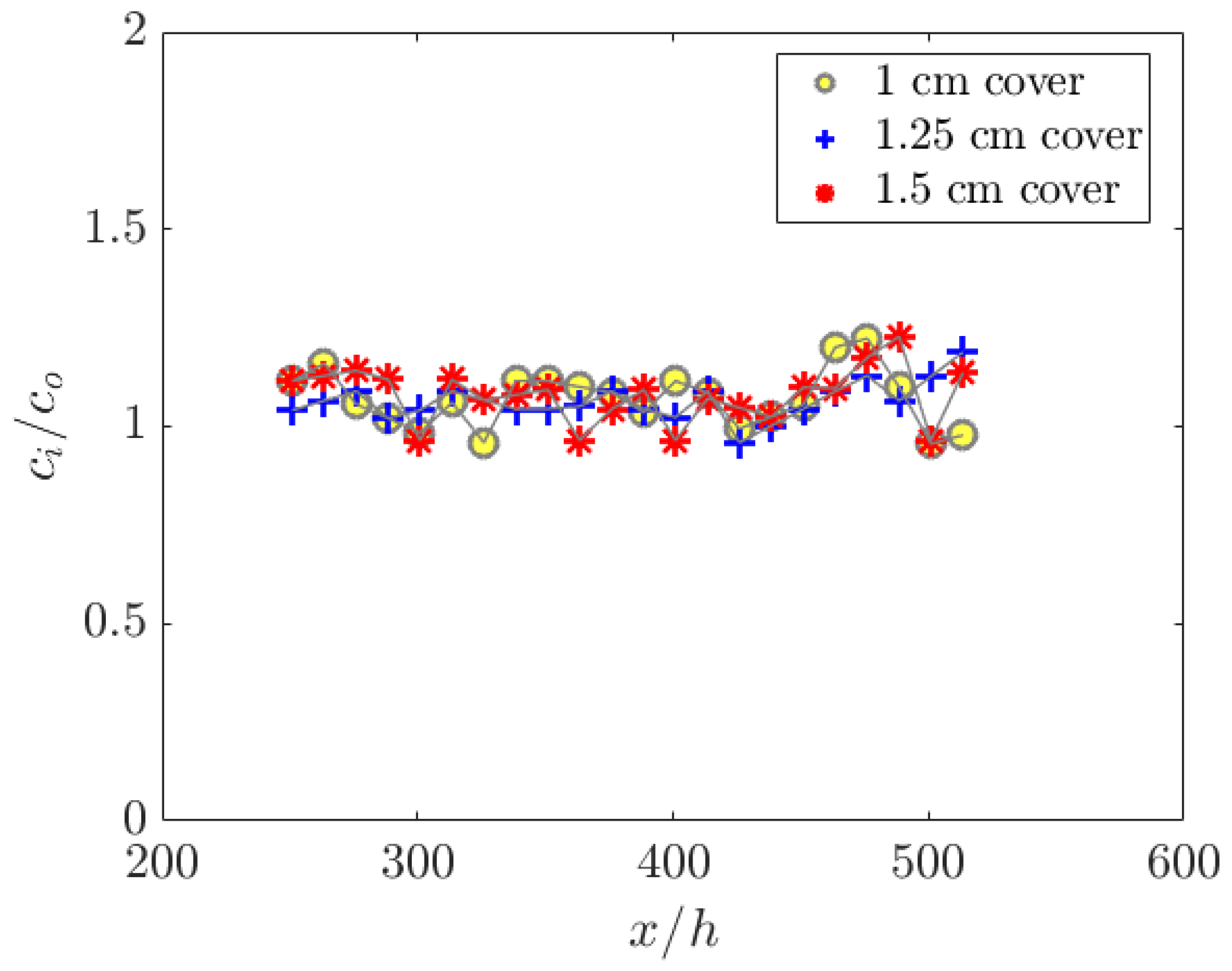
5.3. Results of Different Scales

The scaling law that can be used to study the interaction between water waves and a viscoelastic cover was explained earlier. In this sub-section, analyses are performed to understand whether different scales give similar data or not. To do so, three different thicknesses are considered. The values of $\widehat{E}$ and $\widehat{\eta }$ of all three covers are set to be constant. Then, their responses to four different waves with normalized wavelengths of $56, 76, 100$ and $125$ are numerically simulated.

The computed data are shown in Figure 11. The left panel shows the relative wavenumbers, and the right panel shows the normalized decay rates, respectively. As evident, relative wavenumbers of all three different thicknesses follow each other. There are some differences between them, though the difference is not noticeable. The most possible reason for differences that are observed is the scale effect. The normalized decay rates of different scales also tend to align. Again, they might be different from each other, but the discrepancy between attenuation rates of various scales is not remarkable, which is likely to be caused by the scale effects.

The phase speed variation over the length of the viscoelastic covers, having different thicknesses, is displayed in Figure 12. As seen, the local phase speeds of all three different thicknesses are close to each other. Their mean values are very close to each other. The local values of phase speed of different cases are slightly different from each other. These differences are not significant, and they were expected. It is almost impossible that all three different scales result in highly similar local phase speeds at every point.

5.4. Freshwater Ice Cover Exposed to Water Waves

As mentioned previously, the present computational FSI model is used to replicate the mutual interaction between water waves and freshwater ice. The experiments of Yiew et al. [53] are numerically reproduced by using the present model. Two different ice covers with thicknesses of $1$ and $1.5 \mathrm{cm}$ are modeled.

Wave motion in the ice cover is computed over fifteen cycles. The recorded wave heights are used to compute the attenuation rate, phase speed and wavelength. The viscosity of the ice was not measured in the experiments. To run the problem, tests for different viscosities were run, which helped us to understand the effects of change in viscosity on the attenuation rate, and to find the proper value of the viscosity that can be prescribed for the ice viscosity. Figure 13 shows the effects of change in viscosity on recorded wave heights and the attenuation rate. The results presented in this figure correspond to waves propagating into a cover with a thickness of $1 \mathrm{cm}$. The left panel shows the variation in wave height over the length of the plate for four different considered values for ice viscosity. The data correspond to a wave period of $1 \mathrm{s}$ (${\widehat{\lambda }}_o=125$). As seen, an increase in the normalized viscosity from $1.2\times {10}^7$ to $3.1\times {10}^7$ leads to an increase in the decay rate. However, when the normalized viscosity increases from $3.1\times {10}^7$ to $1.2\times {10}^9$, the attenuation rate decreases. The wave height along the ice cover with a dynamic viscosity of $1.2\times {10}^9$ is very similar to that of an elastic body, i.e., recorded waves have the largest heights at both ends, and they are minimized at the middle of the cover.

The reason for the observed trend for ${\widehat{\alpha }}_i$ as a function of $\widehat{\eta }$ can be explained by using the viscoelastic model employed to solve the solid problem. As was explained earlier, the Maxwell model is used to compute the stresses in the body. The loss moduli of the solid model $G^{″}$ depend on both frequency and relaxation time. The differentiation of $G^{″}$ with respect to relaxation time is

$$\frac{d{G}^{″}}{d\tau }=\frac{G\omega \left(1-{\tau }^2{\omega }^2\right)}{{\left(1-{\tau }^2{\omega }^2\right)}^2}.$$

(35)

The critical relaxation time is

$$\frac{d{G}^{″}}{d\tau }=0 \to \tau =\pm 1/\omega .$$

(36)

For a wave period of 1.0 s, the peak value of the attenuation rate occurs at $\tau$ = 0.16 s, which is equivalent to $\widehat{\eta }=6.3\times {10}^7$. This means that the attenuation rate monotonically increases with the increase in viscosity as long as $\widehat{\eta }$ does not exceed $\widehat{\eta }=6.3\times {10}^7$. However, as normalized viscosity becomes greater than $\widehat{\eta }=6.3\times {10}^7$, the attenuation rate decreases. This well matches with the results observed in Figure 13.

The right panel of Figure 13 shows the computed values of attenuation rate for different prescribed values for $\widehat{\eta }$. The results presented in this figure correspond to a wave period of 0.6 s (${\widehat{\lambda }}_o=56$). As seen, attenuation rate increases with an increase in $\widehat{\eta }$ when $\widehat{\eta }<{10}^8$. For greater values of viscosity, the attenuation rate decreases. This well matches with the theoretical supposition. The peak value of the attenuation rate is expected to occur at $\mathsf{\tau }$ = 0.1 s, which is equivalent to a normalized viscosity of $\widehat{\eta }=6.3\times {10}^7$. A dashed line is plotted in the right panel of Figure 13, indicating the attenuation rate measured in experiments. As can be seen, $\widehat{\eta }=1.28\times {10}^7$ results in an acceptable value of attenuation rate, which is close to the experimental result.

Figure 14 displays the attenuation rate of covers with thicknesses of $1$ (left) and $1.5 \mathrm{cm}$(right). Both experimental (* marker) and numerical data (o marker) are shown in this figure. Additionally, a dashed curve is plotted in each panel, showing the attenuation rates computed by using the theoretical method (which is built based on the Kelvin–Voigt model). The results of the present fluid–solid model are computed by setting the normalized value of the viscosity to be $\widehat{\eta }=1.28\times {10}^7$. The attenuation rates of the dashed solid curves correspond to $\widehat{\eta }=3.2\times {10}^8$ (which is equivalent to a dynamic viscosity of η = ${10}^8$ $\mathrm{Pa}.\mathrm{s}$). It is important to note that the difference between the dynamic viscosity of both models (the present computational one and the theoretical ones) is reasonable because each of them is built by assuming a different behavior for a viscoelastic substance. As seen, the present computational results agree well with experimental data. However, the theoretical model under-predicts the attenuation rate of both ice covers. The theoretical model is less accurate in the prediction of the attenuation rate of the thicker ice. Despite the fact that the approach used to connect the shear stresses and strain rates in each model is different, the present computational model considers the fluid-based energy damping which is absent in the theoretical model.

Dispersion curves of freshwater ice covers are plotted in Figure 15. Experimental and numerical data are shown in this figure. In addition, the results of the theoretical model and open-water dispersion relationship are displayed in this figure. Waves are seen to become shorter under the freshwater ice cover, i.e., markers are below the dash-dotted curve. The experimental and numerical data related to $1.5 \mathrm{cm}$ cover are seen to be in fair agreement, whereas they do not favorably match for the$1 \mathrm{cm}$ cover. The artificial effects related to a thinner cover may be more significant, decreasing the effects of cover on the wavenumber.

The theoretical model is seen to under-predict the wavenumber. This means that this model predicts longer waves (compared to measurements) in the freshwater ice. This matches with the observations of previous researchers, who performed experimental studies, and compared the measured wavelength against the theoretical models. In some of these studies, wavenumber was seen to be under-predict by the pure elastic model, which is likely to be caused by the boundary conditions of the solid body, and the possible nonlinear motion occurring in it (see examples in Sree et al. [34]).

5.5. Sea Ice Cover Exposed to Water Waves

At the final stage, the interaction of water waves with sea ice cover was simulated by using the present computational fluid–solid model. Recorded waves were measured in a recent field experiment, performed by Voermans et al. [33]. The sea ice was modeled by using the scaling law since running simulations for a real-scale condition is not efficient in terms of computational time. The real sea ice had a thickness of $35 \mathrm{cm}$, which was scaled into a $1.25 \mathrm{cm}$viscoelastic cover. Through the field measurements, the recorded wave periods were seen to vary between $5$ and $15$s. For a viscoelastic cover with a thickness of $1.25 \mathrm{cm}$, wave periods varying from $0.85$ to $2.5$ s covered the mentioned range.

Wave amplitude attenuation and dispersion were computed under the ice cover by using the present computational fluid–solid model. To run the simulations, $\widehat{E}$ was prescribed to be 763. This number corresponds to a Young’s modulus of $2\times {10}^9 \mathrm{Pa}$. Different values for $\widehat{\eta }$ were considered, and the related attenuation coefficients were computed. For the tested wave periods, the maximum attenuation rate occurred at $0.13 \mathrm{s}<\mathsf{\tau }<0.4 \mathrm{s}$.

This range corresponds to ${10}^7$ < $\widehat{\eta }$ <$2.85\times {10}^7$. This signifies that an increase in the normalized viscosity leads to an increase in attenuation rate as long as its value is smaller than $\widehat{\eta }~1.9\times {10}^7$ (note that $1.9\times {10}^7$ is the average value of the mentioned range). The maximum attenuation rate is expected to occur when normalized viscosity is close to $1.9\times {10}^7$.

Some runs were first performed by setting the normalized viscosity to be close to the critical value of normalized viscosity. Attenuation rates are seen to be close to field measurements when normalized viscosity is set to be $\widehat{\eta }~1.9\times {10}^6$. The predicted values for attenuation rates are shown in Figure 16. Field data are also plotted in this figure. Attenuation rates and wavelengths of the incoming waves were all normalized. Thus, the field data and the ones found by using the computational fluid–solid model can be compared against each other. In addition, the attenuation rates were computed by employing the theoretical model and setting two different values of $\widehat{\eta }=2.1\times {10}^5$ (corresponding to$\eta$ = ${10}^8 \mathrm{Pa}.\mathrm{s}$) and $\widehat{\eta }=2.1\times {10}^6$ ($\eta$ = ${10}^9 \mathrm{Pa}.\mathrm{s}$) for the ice viscosity. Therefore, the results of the computational fluid–solid model and the theoretical model can be compared with each other. The results of the computational FSI model are seen to be in line with the field data. The results of the theoretical model, however, do not match with the field data. The results of the theoretical model decrease with a high rate when normalized wavelengths are longer than $200 \mathrm{h}$. However, the field data and results of the present computational fluid–solid model do not behave in this way. Instead, they slightly decrease with the increase in wavelength, and at some wavelengths they experience a very sudden and small increase or decrease, which can be caused by different mechanisms. The sudden jumps in the attenuation rate, which can be seen in the results of the present computational data, are likely to be caused by the solid vibration of the cover and the boundary effects. The cover has a finite length with the upstream end being free, which can lead to partial energy reflection from the free end. The largest jump is seen to occur at the longest wave.

The normalized viscosity that has been used corresponds to a dynamic viscosity of $\eta =2.3\times {10}^9 \mathrm{Pa}.\mathrm{s}$. This value is greater compared to the value that was found to provide the greatest accuracy in computation of the attenuation rate of the freshwater ice. The possible reason for this discrepancy is the difference between the problems. First of all, the previous tests are related to freshwater ice, which has a different viscosity compared to sea ice. Second, the freshwater tests were carried out in a wave flume and ice had a finite length. Flume walls and the other two ends of the ice can affect the attenuation rate. This is much different from the landfast ice, where such artificial effects do not contribute to energy dissipation. Finally, the model has been run for a cover with a thickness of $1.25 \mathrm{cm}.$ The scale effects can influence the result of the model as well. Overall, the results presented in Figure 16 confirm that the present computational fluid–solid model can predict the attenuation of a consolidated ice cover with a proper level of accuracy. Its accuracy can also be improved by modifying the setup and also reproducing more field tests, both of which may help us to calibrate the model in future.

Figure 17 illustrates the dispersion curve of the waves propagating through the landfast ice. The results of the present computational fluid–solid model, field data and the predictions given by the theoretical model are plotted in this figure. According to the field data, wavenumbers of waves with greater frequencies become smaller as they travel into the sea ice cover. This has been observed in simulations performed with the present computational fluid–solid model. The results of the computational fluid–solid model and the field data fairly agree. This well shows that the scaling methodology used for reconstruction of waves’ interaction with ice works. In addition, the theoretical model has a reliable level of accuracy in the prediction of the wavenumber.

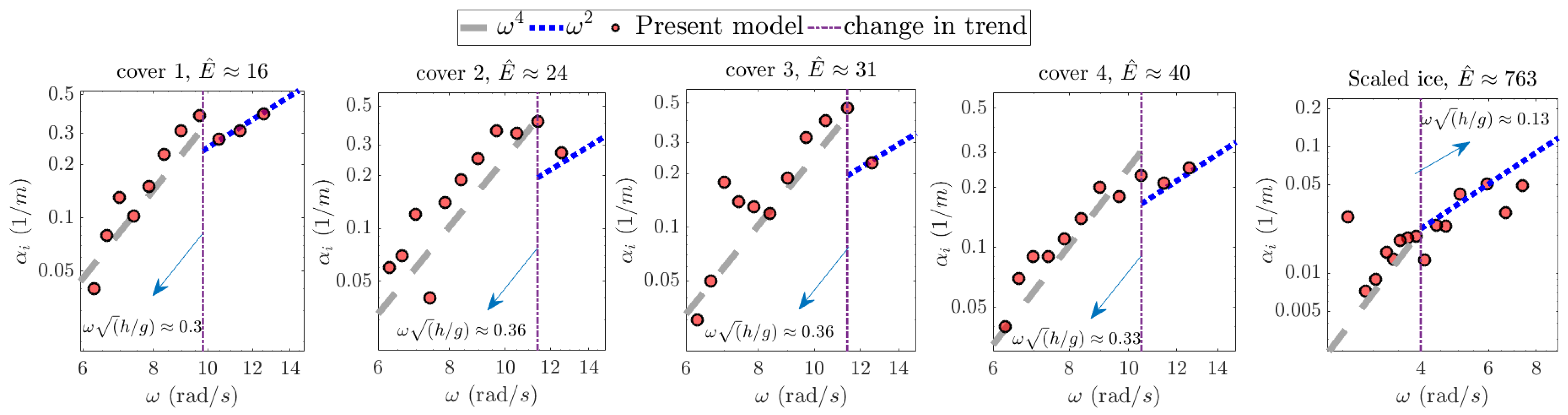
5.6. Dependency of Decay Rates on the Frequency

Results of the present model are interpreted with the aim to understand the dependency of the decay rate on the wave frequency. This can be very helpful in wave climate modeling. As was seen in Figure 14 and Figure 16, the results of experiments deviate from the predictions of a previous theoretical model. This is more significant with longer waves. The dissipation mechanism of the theoretical model is based on the viscoelastic behavior of the material. The difference between its results and those of experiments is perhaps due to the contribution of other dissipation mechanisms, as was explained.

The decay rates predicted by the present model are plotted versus wave frequencies (Figure 18). The decay rate increases under the increase in the wave frequency, but the trend of its increase alters at greater wave frequencies. Assuming there is a turning point at which the decay rate follows a different trend, two different regimes can be introduced. In the first regime (long-wave regime), the decay rate is proportional to ${\omega }^4$, and in the second one (short-wave regime), the decay rate is proportional to ${\omega }^2$. In the first regime, fluid-based energy damping, which can be due to turbulent behavior of the flow or radiation damping, is dominant. Note that the former is not activated in the present research. In the second regime, the solid-based energy damping is likely to be dominant. The frequency that marks the sudden change in behavior of the decay rate as a function of the frequency is termed critical frequency. Dimensionless critical frequency decreases with the increase in elasticity number (note that this is not observed for cover 1; it can be due to the contribution of elastic modes or artificial errors). This signifies that the solid-based decay rate may dFigure minate over a wider range of waves when the solid body has a larger elasticity number.

Similar behavior for the decay rate was observed by Meylan et al. [56], who documented and analyzed decay rates of their field measurements which took place in the Antarctic. They observed that decay rates of wave periods greater than 10 s grow with ${\omega }^4$, but those of shorter waves grow with ${\omega }^2$. Assuming that ice was 1 m thick, the elasticity number of their test would be ≈$590$. The critical dimensionless frequency of their data is ≈$0.2$ which is in between what is found for scaled ice (≈$0.13$) and cover 4 (≈$0.33$), which have elasticity numbers of ≈$763$ and ≈$40$, respectively. This gives more credit to our hypothesis, namely “the critical dimensionless wave frequency decreases with the increase in elasticity number”. Finally, note that the data presented in Figure 18 are very similar to experimental values and such an analysis could be performed using experimental data as well.

6. Conclusions

In the present paper, a computational model was developed to replicate the wave motion of a viscoelastic ice cover interacting with gravity waves. The model solves viscous air–water fluid flow around a flexible body through a strongly coupled FSI approach. Both fluid and solid motions were solved by using a conservative-based approach and the FVM technique was employed to solve the equations governing the fluid and solid motions. The fluid fields were reconstructed by solving the NS equations, and the solid material was simulated through a Maxwell model.

The first set of simulations were run to evaluate the accuracy of the computational fluid–solid model and the related setup. The available flume tests of Sree et al. [34] were numerically reproduced by using the model. The results of simulations, including decay rates and dimensionless wavenumber, were seen to follow experimental data. The present computational approach was seen to be much more accurate than the theoretical model in the computation of the attenuation rate, which provided a promising message about the reliability of the model. Unlike the theoretical model, the attenuation rates predicted by the present computational fluid–solid model do not decrease with the increase in wavelength at a high rate. Instead, they decrease with a very slow rate, which fairly matches the experimental results.

The second set of simulations were run to understand whether the model follows the scaling law or not. Performing simulations for three different ice thicknesses, it was demonstrated that the present computational fluid–solid model obeys the scaling law. The dimensionless attenuation rates and wavenumbers of different scales were seen to align with each other. Small differences were observed, which seem to be reasonable. It is impossible to provide a 100% fitting between the results of different scales as the scale itself can slightly affect simulations.

The model was later used to simulate the interaction between water waves and ice covers. Two sets of tests covering freshwater ice and sea ice were numerically reproduced. The former was tested in a flume, and the other was tested in the real field. Throughout manual fitting, tests were run for different values of viscosity for the freshwater ice. A critical dynamic viscosity was seen to emerge. The attenuation rate was observed to be maximized when this critical viscosity was prescribed for the ice. This behavior was shown to fit with the nature of the Maxwell model, which was used to treat the mechanical behavior of the viscoelastic ice. A proper value for ice viscosity was found, which was used to compute the attenuation rate. The field tests were numerically replicated by scaling the sea ice into a $1.25 \mathrm{cm}$ cover. A proper value for the viscosity was found through a manual fitting. The results of the model were seen to follow the field data. This confirmed that the present computational model can capture the contribution of the different mechanisms to energy dissipation. Such a good performance of the model in the computation of the attenuation rate was seen for the flume tests of Sree et al. [52]. For the modeled sea ice, the viscosity that was found to work with an acceptable level of accuracy was greater compared to that for the freshwater ice. This may be caused by different mechanisms, including the boundary effects, numerical errors, scale effects and the nature of ice, i.e., the difference between the freshwater ice and sea ice. The results computed by the present model are seen not to abruptly decrease with the increase in the wavelength. Based on the validation series, it can be concluded that the present computational model can be used for simulating the interaction between the consolidated ice and water waves.

An analysis was performed to interpret the behavior of decay rate as a function of the wave frequency. Waves were hypothesized to fall into regimes: short-wave regime and long-wave regime. In the short-wave regime, decay rate was demonstrated to grow with ${\omega }^2$, though it was seen to grow with ${\omega }^4$ in the long-wave regime. In a short-wave regime, the viscosity nature of the cover is believed to be the main mechanism modifying waves, though the fluid motion is likely to be the main dissipative mechanism attenuating waves. The ranges of short waves were shown to be increased under the increase in elasticity number, suggesting that solid-based energy damping of a body with a larger elastic modulus may be in effect over a greater range of waves.

All in all, the present computational fluid–solid model was seen to be capable of simulating the interaction between viscoelastic bodies and gravity waves. As the method uses the Maxwell model to link stresses to strains and their rates, the Maxwell model is expected to have an acceptable level of accuracy in computation of the attenuation rate and dispersion under the viscoelastic covers. The computational FSI model can be further calibrated in future. The main concern is the possible effects of the trailing edge on water waves, which can increase the errors in the computation of wavelength and dispersion under the body. This is more probable when waves are longer. In addition, the present computational model can be used to simulate the wave-induced motions of viscoelastic bodies with one fixed end. Such a problem has not been simulated by using the FVM and a viscous fluid assumption, but it has been recently solved by using potential flow theories. Since the present model is less restricted in different aspects, it can capture the frictional energy dissipation and the boundary layer development, which are lacking in the potential flow theory that is currently used for most occasions. Thus, it is recommended to use the present computational FSI model for simulating strongly nonlinear interactive problems, where the high-order approach is expected to obtain further insights into relevant physical and engineering problems.

References

1. Martin, S.; Kaufmann, P. A field and laboratory study of wave damping by grease ice. J. Glaciol. 1981, 27, 283–313. [Google Scholar] [CrossRef]
2. Wadhams, P. Ice in the Ocean; CRC Press: Boca Raton, FL, USA, 2000. [Google Scholar]
3. Parkinson, C.L. A 40-y record reveals gradual Antarctic sea ice increases followed by decreases at rates far exceeding the rates seen in the Arctic. Proc. Natl. Acad. Sci. USA 2019, 116, 14414–14423. [Google Scholar] [CrossRef] [PubMed]
4. Smith, E.K.; Eder, C.; Katsanidou, A. On thinning ice: Understanding the knowledge, concerns and behaviors towards polar ice loss in Germany. Polar Geogr. 2020, 43, 243–258. [Google Scholar] [CrossRef]
5. Melia, N.; Haines, K.; Hawkins, E. Sea ice decline and 21st century trans-Arctic shipping routes. Geophys. Res. Lett. 2016, 43, 9720–9728. [Google Scholar] [CrossRef]
6. Wei, T.; Yan, Q.; Qi, W.; Ding, M.; Wang, C. Projections of Arctic sea ice conditions and shipping routes in the twenty-first century using CMIP6 forcing scenarios. Environ. Res. Lett. 2020, 15, 104079. [Google Scholar] [CrossRef]
7. Huang, L.; Tuhkuri, J.; Igrec, B.; Li, M.; Stagonas, D.; Toffoli, A.; Cardiff, P.; Thomas, G. Ship resistance when operating in floating ice floes: A combined CFD&DEM approach. Mar. Struct. 2020, 74, 102817. [Google Scholar] [CrossRef]
8. Huang, L.; Li, Z.; Ryan, C.; Ringsberg, J.W.; Pena, B.; Li, M.; Ding, L.; Thomas, G. Ship resistance when operating in floating ice floes: Derivation, validation, and application of an empirical equation. Mar. Struct. 2021, 79, 103057. [Google Scholar] [CrossRef]
9. Robin, G.D.Q. Wave propagation through fields of pack ice. Philos. Trans. R. Soc. A 1963, 255, 313–339. [Google Scholar]
10. Squire, V.A.; Moore, S.C. Direct measurement of the attenuation of ocean waves by pack ice. Nature 1980, 283, 365–368. [Google Scholar] [CrossRef]
11. Squire, V.A. Ocean Wave Interactions with Sea Ice: A Reappraisal. Annu. Rev. Fluid Mech. 2020, 52, 37–60. [Google Scholar] [CrossRef]
12. Carolis, D.C.; Desiderio, D. Dispersion and attenuation of gravity waves in ice: A two-layer viscous fluid model with experimental data validation. Phys. Lett. A 2002, 305, 399–412. [Google Scholar] [CrossRef]
13. McGovern, D.J.; Bai, W. Experimental study on kinematics of sea ice floes in regular waves. Cold Reg. Sci. Technol. 2014, 103, 15–30. [Google Scholar] [CrossRef]
14. Huang, L.; Thomas, G. Simulation of wave interaction with a circular ice floe. J. Offshore Mech. Arct. Eng. 2019, 141, 1–9. [Google Scholar] [CrossRef]
15. Kohout, A.L.; Meylan, M.H.; Plew, D.R. Wave attenuation in a marginal ice zone due to the bottom roughness of ice floes. Ann. Glaciol. 2011, 52, 118–122. [Google Scholar] [CrossRef]
16. Voermans, J.J.; Babanin, A.V.; Thomson, J.; Smith, M.M.; Shen, H.H. Wave Attenuation by Sea Ice Turbulence. Geophys. Res. Lett. 2019, 46, 6796–6803. [Google Scholar] [CrossRef]
17. Tran-Duc, T.; Meylan, M.H.; Thamwattana, N.; Lamichhane, B.P. Wave Interaction and Overwash with a Flexible Plate by Smoothed Particle Hydrodynamics. Water 2020, 12, 3354. [Google Scholar] [CrossRef]
18. Li, H.; Gedikli, E.D.; Lubbad, R.; Nord, T.S. Laboratory study of wave-induced ice-ice collisions using robust principal component analysis and sensor fusion. Cold Reg. Sci. Technol. 2020, 172, 103010. [Google Scholar] [CrossRef]
19. Meylan, M.H.; Bennetts, L.; Mosig, J.; Rogers, W.; Doble, M.J.; Peter, M.A. Dispersion Relations, Power Laws, and Energy Loss for Waves in the Marginal Ice Zone. J. Geophys. Res. Oceans 2018, 123, 3322–3335. [Google Scholar] [CrossRef]
20. Collins, C.O., III; Rogers, W.E.; Lund, B. An investigation into the dispersion of ocean surface waves in sea ice. Ocean. Dyn. 2017, 67, 263–280. [Google Scholar] [CrossRef]
21. Squire, V. Of ocean waves and sea-ice revisited. Cold Reg. Sci. Technol. 2007, 49, 110–133. [Google Scholar] [CrossRef]
22. Greenhill, A.G. Wave motion in hydrodynamics. Am. J. Math. 1886, 9, 62–96. [Google Scholar] [CrossRef]
23. Hendrickson, J.A. Theoretical Investigation of Semi-Infinite Ice Floes in Water of Infinite Depth; National Engineering Science Company 711 South Fair Oaks Avenue Pasadena: Pasadena, CA, USA, 1963; NESCONo. P-457/SN-113. [Google Scholar]
24. Wang, R.; Shen, H.H. Gravity waves propagating into an ice-covered ocean: A viscoelastic model. J. Geophys. Res. Space Phys. 2010, 115, C06024. [Google Scholar] [CrossRef]
25. Keller, J.B. Gravity waves on ice-covered water. J. Geophys. Res. Earth Surf. 1998, 103, 7663–7669. [Google Scholar] [CrossRef]
26. Ren, K.; Wu, G.X.; Thomas, G.A. Wave excited motion of a body floating on water confined between two semi-infinite ice sheets. Phys. Fluids 2016, 28, 127101. [Google Scholar] [CrossRef]
27. Li, Z.F.; Wu, G.X.; Ji, C.Y. Interaction of wave with a body submerged below an ice sheet with multiple arbitrarily spaced cracks. Phys. Fluids 2018, 30, 057107. [Google Scholar] [CrossRef]
28. Li, Z.F.; Wu, G.X. Hydrodynamic force on a ship floating on the water surface near a semi-infinite ice sheet. Phys. Fluids 2021, 33, 127101. [Google Scholar] [CrossRef]
29. Xue, Y.Z.; Zeng, L.D.; Ni, B.Y.; Korobkin, A.A.; Khabakhpasheva, T.I. Hydroelastic response of an ice sheet with a lead to a moving load. Phys. Fluids 2021, 33, 037109. [Google Scholar] [CrossRef]
30. Khabakhpasheva, T.I.; Korobkin, A.A. Blunt body impact onto viscoelastic floating ice plate with a soft layer on its upper surface. Phys. Fluids. 2021, 33, 062105. [Google Scholar] [CrossRef]
31. Fox, C.; Squire, V.A. Coupling between an ocean and an ice shelf. Ann. Glaciol. 1991, 15, 101–108. [Google Scholar] [CrossRef]
32. Mosig, J.E.M.; Montiel, F.; Squire, V.A. Comparison of viscoelastic-type models for ocean wave attenuation in ice-covered seas. J. Geophys. Res. Oceans 2015, 120, 6072–6090. [Google Scholar] [CrossRef]
33. Voermans, J.J.; Liu, Q.; Marchenko, A.; Rabault, J.; Filchuk, K.; Ryzhov, I.; Heil, P.; Waseda, T.; Nose, T.; Kodaira, T.; et al. Wave dispersion and dissipation in landfast ice: Comparison of observations against models. Cryosphere 2021, 15, 5557–5575. [Google Scholar] [CrossRef]
34. Sree, D.K.; Law, A.W.-K.; Shen, H.H. An experimental study on the interactions between surface waves and floating viscoelastic covers. Wave Motion 2017, 70, 195–208. [Google Scholar] [CrossRef]
35. Ali, K.; Dutta, H.; Yilmazer, R.; Noeiaghdam, S. On the New Wave Behaviors of the Gilson-Pickering Equation. Front. Phys. 2020, 8, 54. [Google Scholar] [CrossRef]
36. Noeiaghdam, L.; Noeiaghdam, S.; Sidorov, D. Dynamical control on the homotopy analysis method for solving nonlinear shallow water wave equation. J. Phys. Conf. Ser. 2021, 1847, 012010. [Google Scholar] [CrossRef]
37. Noeiaghdam, L.; Noeiaghdam, S.; Sidorov, D.N. Dynamical control on the Adomian decomposition method for solving shallow water wave equation. Ipolytech J. 2021, 25, 623–632. [Google Scholar] [CrossRef]
38. Bai, W.; Zhang, T.; McGovern, D.J. Response of small sea ice floes in regular waves: A comparison of numerical and experimental results. Ocean. Eng. 2017, 129, 495–506. [Google Scholar] [CrossRef]
39. Tavakoli, S.; Babanin, A. Wave energy attenuation by drifting and non-drifting plates. Ocean. Eng. 2021, 236, 108717. [Google Scholar] [CrossRef]
40. Newman, J. Wave effects on deformable bodies. Appl. Ocean. Res. 1994, 16, 47–59. [Google Scholar] [CrossRef]
41. Jiao, J.; Zhao, Y.; Ai, Y.; Chen, C.; Fan, T. Theoretical and Experimental Study on Nonlinear Hydroelastic Responses and Slamming Loads of Ship Advancing in Regular Waves. Shock Vib. 2018, 2018, 1–26. [Google Scholar] [CrossRef]
42. Sun, Z.; Liu, G.-J.; Zou, L.; Zheng, H.; Djidjeli, K. Investigation of Non-Linear Ship Hydroelasticity by CFD-FEM Coupling Method. J. Mar. Sci. Eng. 2021, 9, 511. [Google Scholar] [CrossRef]
43. Lakshmynarayanana, P.; Hirdaris, S. Comparison of nonlinear one- and two-way FFSI methods for the prediction of the symmetric response of a containership in waves. Ocean. Eng. 2020, 203, 107179. [Google Scholar] [CrossRef]
44. Hosseinzadeh, S.; Tabri, K. Hydroelastic effects of slamming impact Loads During free-Fall water entry. Ships Offshore Struct. 2021, 16 (Suppl. S1), 68–84. [Google Scholar] [CrossRef]
45. Huang, L.; Ren, K.; Li, M.; Tuković, Ž.; Cardiff, P.; Thomas, G. Fluid-structure interaction of a large ice sheet in waves. Ocean Eng. 2019, 182, 102–111. [Google Scholar] [CrossRef]
46. Huang, L.; Li, Y. Design of the submerged horizontal plate breakwater using a fully coupled hydroelastic approach. Comput. Civ. Infrastruct. Eng. 2021, 37, 915–932. [Google Scholar] [CrossRef]
47. Yu, J.; Rogers, W.E.; Wang, D.W. A Scaling for Wave Dispersion Relationships in Ice-Covered Waters. J. Geophys. Res. Oceans 2019, 124, 8429–8438. [Google Scholar] [CrossRef]
48. Cardiff, P.; Karač, A.; Jaeger, D.P.; Jasak, H.; Nagy, J.; Ivanković, A.; Tuković, Ž. An open-source finite volume toolbox for solid mechanics and fluid-solid interaction simulations. arXiv 2018, arXiv:1808.10736. [Google Scholar]
49. Jacobsen, N.G.; Fuhrman, D.R.; Fredsøe, J. A wave generation toolbox for the open-source CFD library: OpenFoam®. Int. J. Numer. Methods Fluids 2012, 70, 1073–1088. [Google Scholar] [CrossRef]
50. Jacobsen, N.G. Waves2foam Manual; Deltares: Delft, The Netherlands, 2017; p. 570. [Google Scholar]
51. Huang, L.; Li, Y.; Benites, D.; Windt, C.; Feichtner, A.; Tavakoli, S.; Davidson, J.; Paredes, R.; Quintuna, T.; Ransley, E.; et al. A review on the modelling of wave-structure interactions based on OpenFOAM. OpenFOAM J. 2022, 2, 116–142. [Google Scholar] [CrossRef]
52. Sree, D.K.; Law, A.W.-K.; Shen, H.H. An experimental study on gravity waves through a floating viscoelastic cover. Cold Reg. Sci. Technol. 2018, 155, 289–299. [Google Scholar] [CrossRef]
53. Yiew, L.; Parra, S.; Wang, D.; Sree, D.; Babanin, A.; Law, A.W.-K. Wave attenuation and dispersion due to floating ice covers. Appl. Ocean Res. 2019, 87, 256–263. [Google Scholar] [CrossRef]
54. Squire, V.A.; Dixon, T.W. An analytical model for wave propagation across a crack in an ice sheet. In Proceedings of the 10th International Symposium on Offshore and Polar Engineering, Seattle, WA, USA, 28 May–2 June 2000; Chung, J., Ed.; International Society of Offshore and Polar Engineers: Cupertino, CA, USA, 2000; Volume 1, pp. 652–655. [Google Scholar]
55. Squire, V.A.; Dixon, T.W. How a region of cracked sea ice affects ice-coupled wave propagation. Ann. Glaciol. 2001, 33, 327–332. [Google Scholar] [CrossRef]
56. Meylan, M.H.; Bennetts, L.G.; Kohout, A.L. In situ measurements and analysis of ocean waves in the Antarctic marginal ice zone. Geophys. Res. Lett. 2014, 41, 5046–5051. [Google Scholar] [CrossRef]
Figure 1. A schematic showing the concept of wave–ice interaction. Water waves propagate through a viscoelastic cover. Here, a Kelvin–Voigt model represents the solid motion occurring in the ice layer.
Jmse 10 01220 g001
Figure 2. A sketch of the computational domain used to numerically reproduce the interaction between water waves and a viscoelastic cover. A Maxwell model, as shown in the circle, is employed to calculate the stresses emerging in the solid domain.
Jmse 10 01220 g002
Figure 3. The mesh used to solve the wave–ice interaction in the present research. The structure of the mesh generated in the fluid domain is shown on the left, and the one related to the solid domain is shown on the right. Zoomed-in views are indicated in the circles.
Jmse 10 01220 g003
Figure 4. Measured values of storage (circles) and loss (triangles) moduli. The upper row shows the mechanical properties of covers 1 (left) and 2 (right), and the lower row shows the mechanical properties of covers 3 (left) and 4 (right). The data were measured by Sree et al. [34].
Jmse 10 01220 g004
Figure 5. Wave motion at two different points of the viscoelastic cover. The data are related to the waves with a period of 0.65 s. Here, H i n is the height of the incoming wave.
Jmse 10 01220 g005
Figure 6. Reduction in the wave motion along the viscoelastic cover exposed to water waves. The red and the blue curves show the data found by free–free and free–fixed conditions assumed for the solid body.
Jmse 10 01220 g006
Figure 7. Recorded local phase speed at different points. The data found through computations are shown with the circle markers. The dashed red line is the reference line.
Jmse 10 01220 g007
Figure 8. Snapshots presenting the water surface elevation profile around the viscoelastic cover at different time steps. The red curve displays the solid cover interacting with water waves.
Jmse 10 01220 g008
Figure 9. Comparison between computational and experimental decay rates. Experimental and computational data are respectively shown by yellow and blue markers. The black plot shows the predictions of Equation (5). The experimental data are taken from Sree et al. [52].
Jmse 10 01220 g009
Figure 10. Dispersion curves of waves traveling into uncovered water (dash-dotted red curve) and covered water (markers and solid curves). Experimental and computational data are respectively shown by yellow and blue markers. The black plot shows the predictions of Equation (5). The experimental data are taken from Sree et al. [52].
Jmse 10 01220 g010
Figure 11. Results of different scales found by using the present computational model. Left and right panels respectively show the dispersion and attenuation rates at different incoming wavelengths.
Jmse 10 01220 g011
Figure 12. Phase speed of waves traveling through viscoelastic covers with different scales. Results are found by using the present computational model.
Jmse 10 01220 g012
Figure 13. Effects of dynamic viscosity on the wave decay along an ice cover. Left panel shows the wave decay over the length of the cover, and right panel shows the computed attenuation rates (found through exponential curve fitting). The horizontal line refers to the value reported in experiments of Yiew et al. [53].
Jmse 10 01220 g013
Figure 14. Comparison between decay rates given by the present computational model and the experimental values presented in Yiew et al. [53]. The dashed curves show the decay rate vs. open-water wavelength curves constructed by using Equation (5). Left and right panels respectively show the results corresponding to the ice covers with thicknesses of 1 and 1.5 cm.
Jmse 10 01220 g014
Figure 15. Dispersion curves of waves propagating in the freshwater ice (dashed curve and markers) and open-water conditions (dash-dotted blue curve). Experimental data are taken from [53]. The dashed curve is constructed using Equation (5).
Jmse 10 01220 g015
Figure 16. Comparison between decay rate given by the model (o markers) and the measured data (* marker) in the field tests of Voermans et al. [33]. The dashed and dotted curves show the decay rate vs. open-water wavelength curves constructed by using Equation (5).
Jmse 10 01220 g016
Figure 17. Dispersion curves of waves propagating in the covered (markers and dashed curve) and uncovered sea (dash-dotted blue curve). Field data (* markers) are taken from [33]. The dashed curves show the dispersion curve constructed using Equation (5). The results of the present model (circle markers) are found by running the model for small-scale ice.
Jmse 10 01220 g017
Figure 18. Decay rates as a function of wave frequency. Panels show the data found using the present model.
Jmse 10 01220 g018
Publisher’s Note: MDPI stays neutral with regard to jurisdictional claims in published maps and institutional affiliations.