Laboratory Experiments on Ice Melting: A Need for Understanding Dynamics at the Ice-Water Interface

Abstract

The ice-ocean interface is a dynamic zone characterized by the transfer of heat, salinity, and energy. Complex thermodynamics and fluid dynamics drive fascinating physics as ice is formed and lost under variable conditions. Observations and data from polar regions have shed light on the contributions that oceanic currents, meltwater plumes, subglacial hydrology, and other features of the ice-ocean boundary region can make on melting and transport. However, the complicated interaction of mechanisms related to ice loss remain difficult to discern, necessitating laboratory experiments to explore fundamental features of melting dynamics via controlled testing with rigorous measurement techniques. Here, we put forward a review of literature on laboratory experiments that explore ice loss in response to free and forced convective flows, considering melting based on laminar or turbulent flow conditions, ice geometries representing a range of idealized scenarios to those modeling glaciers found in nature, and features such as salinity and stratification. We present successful measurement techniques and highlight findings useful to understanding polar ice dynamics, and we aim to identify future directions and needs for experimental research to complement ongoing field investigations and numerical simulations to ultimately improve predictions of ice loss in our current and evolving climate.

1. Introduction

1.1. Background and Motivation

Glacial melting in the polar regions due to anthropogenic climate change is one of the predominant mechanics of rising sea level [1,2]. At the Greenland and Antarctica ice sheets, ice melting has increased rapidly since the 1990s. Ice loss at the Greenland Ice Sheet quadrupled from the 1992–2001 period to the 2002–2011 period [3], and half of the sea level rise from 1972–2018 attributed to Greenland melting occurred within the last decade [4]. The 2018 Fourth National Climate Assessment by the U.S. Global Change Research Program details the negative effects sea level rise will have in the United States [5] due to ocean encroachment on coastal regions, increasingly destructive storm surges, effects on ecosystems from altered nutrient and sediment cycles, and changes in oceanic and atmospheric circulations.

Oceanic effects can vary locally based on water temperature and salinity, affecting melting. Further, the presence of subglacial plumes, underlying ocean currents, fjord topography, and fjord circulation processes including tides, internal waves, atmospheric forcing, and freshwater buoyancy forcing have individual and coupled impacts. In Greenland, heat, salt, and freshwater exchange to and from marine terminating glaciers primarily occurs in narrow, deep fjords. While observations of surface elevation and ice mass of glaciers are determined via data from satellite missions such as the Ice, Cloud, and Land Elevation Satellite-2 (ICESat-2) [6] and Gravity Recovery and Climate Experiment-Follow On (GRACE-FO) satellite [7], in situ observations at the ice shelf-ocean boundary layer are more difficult to obtain. However, these observations are key to informing the needed parameterizations for improving the accuracy of numerical ice melting simulations and subsequent sea level rise predictions.

In the field of ice sheet modeling, melting predictions are highly empirical. Early models focused on one-dimensional dynamics of ocean-ice interactions (e.g., [8,9,10]) and buoyant plumes (e.g., [10,11]). While these models have improved in complexity and resolution to encompass two-dimensional dynamics [12,13,14,15], refinement of model inputs is needed to improve the accuracy of future sea level predictions based on melting of ice features experiencing myriad flow-ice dynamics. Common theories to determine melting rates include the buoyant plume theory, the flux-gate method, and the coupled plume-melt parameterization.

Buoyant plume theory is used to obtain estimates of submarine melt [11,16,17]. This model uses far-field ocean measurements, which are collected away from the ice face and are easier to obtain in field studies. However, as summarized by [18], buoyant plume theory requires subglacial conduit geometry, the magnitude of discharge, and empirical constants that remain untested. The flux-gate (i.e., fjord budgets) method [19,20] uses conservation of heat, salt, and mass to obtain freshwater fluxes at the terminus region of the ice by using far-field data. While the method does not require near-glacier data to obtain submarine melt, it does need dense ocean measurements [18]. Additionally, this method does not capture storage of heat, salt, or mass in the conservation budgets, nor other uncertainties such as when circulation within the fjord is unsteady [20]. Melt rates and near-ice velocities can be coupled with buoyant plume theory with the submarine melt parameterization of [21] via a plume-melt parameterization [11]. The widely-used melt parameterization of [21,22,23] (commonly referred to as the three-equation model) uses near-ice values (velocity, temperature, and salinity) to determine heat and salt transfer at the turbulent boundary layer.

Jackson et al. [24] investigated ambient melting at the terminus of a tidewater glacier in Alaska and found melt rates to be up to 100 times greater than those predicted by current theory. Ref. [24] updated the coupled plume-melt parameterization to account for the higher melt rates observed in field work campaigns. For instance, the parameterization uses turbulent transfer coefficients for heat and salt, a drag coefficient, and other standard values for tidewater glaciers that are commonly used (e.g., [11,15,25]). Ref. [24] noted these coefficients are empirical values from horizontal ice geometries such as sea ice and ice shelves from [22,26], but it remains unknown whether these are accurate for near-vertical ice interfaces. For the coupled plume-melt parameterization, ref. [24] suggests adjusting the coefficients to match observed melt rates. Furthermore, they made another modification by adding the effect of an external horizontal velocity to the buoyant plume theory. However, ref. [24] noted they are unsure which adjustments are correct without additional work.

Similarly, ref. [18] found observed melt rates to be twice as high compared to theoretical predictions at the tidewater LeConte Glacier in Alaska. They suggested complex feedback loops exist that influence melting but that are not captured in melting simulations using buoyant plume theory or the flux-gate method. Regarding subglacial plumes released at ice-ocean interfaces, ref. [27] presented a review addressing the need for more validations of model parameters. Overall, there is still much uncertainty regarding how oceanic, glaciological, and atmospheric processes affect melt rates at glacier termini. Observations that could inform these theories are difficult and costly to perform, and it is challenging to isolate the effects of different measured parameters on melting.

It is imperative to have accurate predictions of glacier ice loss and subsequent sea level rise. Clearly, mechanisms of ice loss are complex and intertwined, leading to difficulties in developing numerical models that accurately portray the driving physics [28]. While there have been substantial field campaigns (e.g., [18,29,30,31,32] that have provided submarine melting and near-ice turbulence, temperature, oxygen, and salinity measurements, we still face a lack of understanding of the relative importance of various mechanisms that drive ice loss in polar environments, thus necessitating laboratory experiments to investigate fundamental components of melting phenomena.

Several studies exploring ice solidification, including the impact of convective currents on ice formation [33,34], aqueous salt solutions solidified from above [35], turbulent measurements during ice growth [36], ice formation in a differentially heated cavity [37], and formations on lake ice from brine rejection [38] (in review) have been conducted, mostly with applications for sea ice growth. In addition, there are several experiments exploring melting of ice in air to explore, for example, hailstones (i.e., ice spheres) in an air stream [39], ice cubes in air flows at a wide range of temperatures [40], and ice in rectangular, cylindrical and conical forms in air of varying velocities [41]. Ref. [42] provides a recent review of experiments of hailstones, graupel, ice crystals, and snowflakes melting in air. While this type of work is not focused on polar melting, the experimental techniques and findings are useful for expanding our understanding of the parameter space surrounding mechanically-induced melting from moving fluids.

Here, we present a review of the literature encompassing laboratory experiments of ice melting and ice loss as a function of ambient water temperature, salinity, ice geometry, and associated fluid dynamics. Furthermore, a focus is made on the experimental facilities and measurement techniques such as particle image velocimetry (PIV), particle tracking velocimetry (PTV), laser-induced fluorescence (LIF), laser Doppler velocimetry (LDV), acoustic Doppler velocimetry (ADV), and shadowgraphy, along with dye visualizations of meltwater and stratification. While we acknowledge that not all of these works were motivated by glacial melting, this review serves to explore individual contributors to melting processes and the interactions of mechanisms that drive melting. To our knowledge, the only other review focused on experimental ice work is that of [43]. We have expanded upon this review to include work not presented previously and all subsequent work completed in the last three decades. While we focus on the experimental aspects of recent ice melting work and what future ice-related experiments should address in the context of polar dynamics linked with sea level rise, we would be remiss not to mention a recent review of modeling parameterizations of thermodynamic ablation at ice-ocean interfaces [44].

1.2. Key Concepts and Definitions

At the ice-ocean interfaces in Greenland, iceberg calving and submarine melting occur at tidewater or marine-terminating glaciers and are responsible for between one-third and one-half of the total annual ice mass loss to the ocean [45]. In Antarctica, the phrase ice sheet describes regions where the ice is still grounded, whereas the ungrounded extensions of ice are the floating ice shelves that encompass three-quarters of Antarctica’s coast [46]. Following Archimedes’s principle, as these ice shelves melt, they do not cause sea level rise, but they do contribute significantly to ice sheet instability and ice flow towards the ocean. While a portion of the mass loss is due to increased air temperatures in the polar regions [47], submarine melting and grounding line retreat is attributed to the rapid loss of ice shelves and glaciers [48,49,50,51,52,53]. Moreover, warming subsurface waters are enhancing ice mass loss [54].

In glacier ice formed naturally, pressurized air bubbles are frozen within the ice structure [55]. The air trapped within the ice influences fluid flow via “jetting” behavior as it is released upon melting [56,57]. Few laboratory experiments [58] and field measurements [59] isolate the effects of pressurized bubbles in ice melting. Similarly, synthetic or laboratory-made ice may also contain bubbles, though these bubbles are typically not pressurized as in glacier ice [60]. Several studies note that even without a strong gradient between the bubble pressure and ambient hydrostatic pressure, bubbles frozen within ice can influence the roughness of the ice during the melting process [61] and affect flow patterns upon release [62,63]. In order to reduce the complexity of laboratory measurements due to the presence of bubbles, many of the experimental studies presented herein used a variety of freezing techniques to produce bubble-free ice (e.g., [64,65,66]).

Another ice surface property that may significantly influence flow dynamics at ice-water interfaces is the presence of ice scallops or morphological features on the ice surface. Scallops are often found on various types of ice faces, including those on glaciers, icebergs, sea ice, and river ice (e.g., [67]). Scallops are likely to enhance turbulent heat transfer by increasing drag [68]. Most of the experimental studies presented herein use initially flat ice and comment on how more realistic ice textures in experiments would have influenced melting rates.

The presence of salt can influence mechanisms of ice loss. Melting will occur when the temperature of the fluid (i.e., fresh water, salt water, air) adjacent to ice is above the melting temperature of the ice, or approximately 0 °C (for fresh water at atmospheric pressure), and thus heat transfer occurs, causing a phase change from solid ice to liquid water. However, dissolution can occur when ice is in contact with saline water whose temperature is near or below the melting point of ice, due to reduction in the melting temperature from the salinity [69]. The difference between when dissolution or melting occurs has seen little focused attention in melting experiments, except by a few authors [70,71,72,73].

Convection in water is different from convection in other fluids because of the unique density maximum of water at approximately 4 °C when water is in a liquid state. By contrast, other fluids typically strictly see an increase in density with a reduction in temperature as the transition from liquid to solid state occurs. Intuition would indicate the warmer fluid to rise, such as the case with warm air, but this does not always hold for a water-based system. Density increases monotonically with temperature for water temperature below 4 °C.

This behavior of the density surrounding the temperature of maximum density (TMD) results in different configurations of stable or unstable stratified layers. For scenarios with floating ice, a stable density stratification exists for which 0 °C $<T<4$ °C, where T indicates water temperature, whereas for $T>4$ °C, an unstable lower density stratification exists, as shown in Figure 1. Similarly, ice affixed at the bottom of a water tank will generate an unstable stratification in the layer adjacent to the ice for 0 °C $<T<4$ °C, whereas the upper layer ($T>4$ °C) will remain stably stratified.

When the density stratification is unstable, such that fluid of a greater density is positioned above fluid of a lower density, convective motion will occur, as detailed in the following papers. If the water temperature is greater than 4 °C, the free convection buoyancy force will become inverted. The result is a dual flow occurring; however, if the temperature is significantly greater than 4 °C this dual flow will be absent, and classic boundary layer flow will be observed along interfaces. The generation of convective motion is influential in ice melting systems as heat transfer through convective flows will subsequently drive the flow of meltwater away from the ice or carry ambient water warmer than the meltwater toward the ice. Note that, when water salinity increases, the TMD decreases to a value lower than 4 °C. The change results in effects on the buoyancy forces at ice-water interface as described in [74].

Here we introduce some of the dimensionless parameters considered throughout this review. The parameters characterize the flow and melting phenomenon at the ice-water interface in experiments. A key dimensionless parameter used in many of the ice melting experiments centered upon free convection is the Nusselt number, $Nu$. The Nusselt number provides a ratio of convective to conductive heat transfer and is used to determine which heat transfer mechanism is dominant. The Rayleigh number, $Ra$, is a nondimensional number that describes the stability criteria for a fluid in a horizontal layer (e.g., beneath a horizontal ice sheet) in buoyancy-driven or convective flows. The Rayleigh number characterizes whether the flow is laminar or turbulent. The Rayleigh number has been used to study melting of ice spheres (e.g., [75]), horizontal ice (e.g., [76]), and vertical ice (e.g., [77]). The Grashof number, $Gr$, is the ratio of the buoyancy to viscous force, commonly used in studies of natural convection. The Prandtl number, $Pr$, is the ratio of momentum diffusivity to thermal diffusivity. The Rayleigh number is the product of the Grashof and the Prandtl numbers. The Reynolds number, $Re$, is the ratio of the inertia to viscous force. In melting experiments, it has been used to represent the strength of turbulent shear flow (e.g., [65]).

1.3. Overview

The paper is structured as follows: Section 2 presents experimental literature on melting and flows produced in free convection conditions, while Section 3 explores melting in forced convection generated from buoyant plumes, circulations, turbulence-producing apparatus, and other controlled flows. Section 4 discusses the use of laboratory ice melting studies to improve accuracy of large scale ice melting models as well as modern laboratory techniques to perform high quality and productive ice melting experiments. Section 5 provides a brief conclusion on the work presented in this review. We also present Appendix A with a listing of the experiments.

2. Free Convection Experiments

Experimental ice studies starting in the 1960s focused on ice melting in conditions of free convection absent of any forced shear, oscillatory, or turbulent flows. Convection is flow driven by a temperature, and subsequently density, gradient; convective flows transfer heat as a result. In the free convection experiments we explore below, the temperature and resulting density differences between the ice and adjacent ambient water promote free convection. While there are no mechanically forced flows in these scenarios, unstable density stratifications generated by thermal gradients drive currents, circulation cells, and turbulence.

2.1. Horizontal Ice Sheets

Horizontally-oriented ice exists in the polar regions as sea ice, as undercuts or ungrounded extensions of glaciers, or bottoms of icebergs. Sea ice is of particular interest in studying polar melting. The less sea ice that exists in the oceans of the polar regions, the more the albedo effect is lessened, and the more solar radiation is absorbed into the exposed dark ocean water. The result is a feedback loop in which reduction of sea ice causes water temperatures to rise. This subsequently leads to less sea ice solidification during the fall and winter months, when the sea ice would typically recharge itself, and thus faster melting of existing sea ice in the summer.

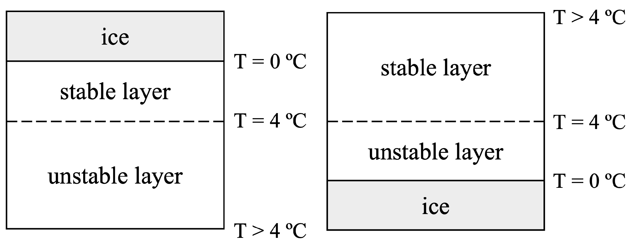
Townsend [78] studied the effect of convective motion in an underlying unstable layer of fluid on a stable, stratified layer above in a small facility with a 30 cm by 30 cm square base filled to 15 cm with distilled water. The upper stable layer of water was maintained at 25 °C using an overhanging heated plate while the bottom of the tank was chilled to produce a thin layer of ice (Figure 2). Observations of dye streaks and suspended particles showed the water above the ice to be stable initially. As the ice melted and approximately 0 °C meltwater rose from the bottom ice sheet, overturning occurred in a thin layer above the ice, and rising buoyant columns were visible. The buoyant columns rose to a stable stratification region of 3.2 °C before spreading horizontally at this depth. While this work lacked direct applications to glacier melt, they provided one of the first fundamental studies of ice melting.

Myrup et al. [79] used an ice cube (1 ft. sides and cooled by a copper plate from below) overlain by fresh water with the intent of better understanding natural convective systems. Three regions were observed: a boundary layer, a convective layer, and an upper layer where convective currents did not penetrate. The cold buoyant plumes in the convective layer rose until they reached a neutrally buoyant layer, at which point they spread horizontally in a wavy motion, suggesting the presence of gravity waves. By analyzing thermocouple temperature data, it was determined the upper inversion layer was cooled by conduction, heat was carried by convection in the convection layer and by conduction to the boundary layer, and this heat was then converted to latent heat as the ice melted.

Adrian [80] performed similar fundamental experiments to [78,79] of turbulent, statistically steady convection over a horizontal ice surface submerged in water and beneath a stably stratified layer in a 33.3 cm by 33.3 cm square base tank. Dural upper and lower plates maintained the water temperature with the top plate set to either 23.3, 25.6, or 33.6 °C, resulting in the convection layer thickness varying slightly based on temperature. The lower plate was kept near 0 °C. An LDV measured vertical velocity of the fluid flow, while thermistors embedded in the ice recorded the temperature. Observations revealed convection in a horizontal layer at a constant depth and a stratified, stable layer where internal gravity waves propagated.

Seki et al. [76] performed experiments that melted horizontal ice overlain by fresh water that was at an initial temperature of 0 °C. A copper plate heated between 1 and 15 °C was located above the horizontal water layer to investigate free convective heat transfer. The apparatus measured 150 mm by 150 mm with a height of 25 mm. They noted the TMD of water played a significant role in the development of free convection and heat transfer in the water layer for T≤ 8 °C.

The following works were setup such that the water was either beneath the ice for broad planes of ice, or surrounded ice cylinders for complementary experiments, as compared to the previous studies with only bottom-mounted horizontal ice sheets. While ice cylinders have a simplified, symmetrical shape that would not be found in nature, results of flow patterns around the ice can be applied to scenarios with various natural ice geometries, such as icebergs and sea ice. In laboratory experiments, ref. [81] studied the free convection of water under a horizontal slab of ice to understand melting that would occur at the underside of an iceberg or sea ice. Experiments were performed in a slightly larger tank than in prior studies, with a 45 cm by 45 cm square base and water depth of 75 cm. The ice was located at the upper surface of water with a salinity of 37.6‰ using a NaCl solution, differing from the previous two studies that used fresh water. The far-field (i.e., ambient) temperature at the bottom of the tank was maintained constant at approximately 0 °C. Ref. [81] identified three regions of heat transfer: a diffusive boundary layer at the ice-water interface where the temperature increase was linear and salinity nearly approximated the far-field value, an unstable boundary layer of double-diffusive convection below the diffusive boundary layer, and a thermal convection layer in the far-field. Double-diffusive convection occurs when two different density gradients result in different rates of diffusion and a finger-like pattern of density develops. Double-diffusive convection drives mixing of salinity and heat flux at the ice-water boundary [82,83]. A one-dimensional model of ice melting in conditions of purely diffusive heat transfer found the ice to melt approximately twice as fast in the laboratory convective case.

Gebhart et al. [84] conducted experiments of horizontal ice slab melting from below in water to understand the melting of circular sea ice. The ambient water conditions ranged from temperatures of −1.75 to 3 °C with a salinity of 35‰. Observations of passive seeding particles dispersed in the water showed the flow below the ice to move radially inward toward the center of the ice across the entire temperature range. An outward moving horizontal layer of flow was observed directly below the inflow layer, which moved deeper with increasing ambient water temperature. Ref. [84] noted that the buoyancy force has two diffusive components, thermal and saline, which depend on the local temperature and salinity. Lastly, the local melt rate for all temperatures was found to be higher at the edges of the ice sheet as compared to the center.

To understand the melting of glaciers, ref. [85] investigated the melting of ice in 35‰ (by weight) saline water at ambient water temperatures ranging from 1.8 to 25.0 °C. The geometry of the ice used in the experiments consisted of horizontal ice cylinders and ice plates inclined at angles from 0 to 75 degrees to the horizontal plane. Visualizations were recorded of melting occurring above and below the inclined ice plates and around the horizontal cylinder. Ref. [85] determined the melting heat transfer coefficient from the local melting velocity via analysis of photographs of the melting ice. Results showed the melt rate to increase monotonically with the ambient water temperature for both ice geometries, whereas the melt rate was nearly independent of the angle of inclination for the ice plate.

Fukusako et al. [86] investigated the melting of a horizontally-oriented ice cylinder in ambient water of constant salinity of 35‰, while varying temperature from 2.8 to 20.3 °C in initially quiescent conditions. Visualizations of aluminum powder seeding particles illuminated by a He-Ne laser showed laminar bidirectional flow at the lower region of the ice and upward turbulent flow in the upper region, consistent with prior findings. The velocity at which the ice melted was found to increase linearly as the ambient water temperature increased. Ref. [87] investigated the free convection melting of a horizontal ice cylinder varying ambient water salinity (5 to 35‰) and temperature (1.8 to 24.0 °C). Visualization of flow patterns around the ice was accomplished by seeding the water with aluminum powder particles and illuminating the particles with a He-Ne laser sheet. PIV, which was concurrently under development and could potentially have been used in this configuration to obtain quantitative velocity measurements from the visualizations, was not used. Three regimes of flow were observed: the density inversion of the saline water where the flow around the cylinder was upward, a lower laminar and unidirectional portion, and a turbulent upper region.

Motivated to understand the melting of glaciers in sea water, ref. [88] melted horizontal ice plates into a calcium chloride aqueous solution from above. The experiments were described as ice plates melting spontaneously and the temperature decreasing at the melting front despite no initial difference between the ice and water with the temperature for both at the beginning of the experiment set at −5 °C. Flow visualizations revealed natural convection at the melting front, which was dominated by the concentration gradient in this region. A two-dimensional numerical model was used to calculate the theoretical melting, which was comparable to the experiments with a difference of less than 30%.

In direct numerical simulations (DNS) and laboratory studies, ref. [89] investigated the effect of turbulent convection on melt rates beneath a horizontal ice layer. The experimental facility was a Plexiglas tank, insulated with a layer of Styrofoam and filled with tap water. An ice block (made from distilled water) was positioned at the water surface. Scaling laws were determined to understand the relationship between the melt rate and the far-field temperature. Results revealed the melt rate increased two orders of magnitude with a far-field temperature of 4 to 8 °C. The results also showed a stably stratified diffusive layer that insulated the ice from the warmer, turbulent layer when the far-field temperature was below 8 °C. The stratification of this layer was not present when the far-field temperature was above 8 °C. The flow structures and melt rate results from the DNS were found to agree with the laboratory experiments.

Yen and Galea [90,91] performed unique experiments of fixed vertical ice cylinders in a cylindrical apparatus with heating from above. The top surface of the ice was melted, which subsequently resulted in a deepening horizontal layer of water at the top of the ice over time. These experiments aimed to determine when the mode of heat transfer to the ice changed from conduction to convection in the water layer. A cold plate was located at the bottom of the tank, while a warm plate was located at the top. The upper warm plate was varied in temperature from 4.06 to 39.90 °C and the initial ice temperature was varied from −6.5 to −14 °C. The initial ice temperature did not significantly affect the onset of convection. The time at which convection began could be determined from when the inflection point occurred in the data curve of water-ice interface position to time, or at the time when the temperature profile of the water layer, measured by thermistors, diverged from a linear distribution.

Wagman and Catania [92] performed a study to understand how subglacial hydrology affects the motion of ice in Antarctic ice streams. The ice streams were modelled using a silicone polymer that substituted as ice to simplify the experimental design. The surrogate ice was located over a thin water layer in the experiments. This model allowed the basal sliding of ice flow to be studied in a simplified setup with surrogate ice. Results showed the stability of the ice-stream is influenced by changes in basal lubrication.

Stepanova and Chaplina [93] investigated the rotation of ice disks placed on a solid surface and on water at a temperature of 20 °C. The ice was dyed for flow visualization. The threshold depth of water for the rotation to occur was 3 cm. While some key details of the experimental setup such as water salinity were not provided, the ice rotation was reported to be slower in saltwater compared to in fresh water. For the water surface experiments, the ice mass loss was found to be exponential with time. Ice rotation was found to be caused by vortex flow underneath the ice. The rotation velocity increased with the water temperature in the reservoir. Rotation did not occur at water temperatures of 5 °C and below due to effects of the TMD of water.

A few other papers also considered ice melting via laboratory experiments, but the applications and temperature ranges were not focused on ice melting in natural scenarios. For example, ref. [94] investigated natural convection due to proximity to the TMD above ice overlain by a recalculating reservoir with water of a temperature of 70 °C. Accompanying numerical simulations closely matched the experimental results. Ref. [95] performed experiments to understand how compositionally-driven melting occurs in magma chambers, specifically to explore how ice and wax melted under or over a hot aqueous solution of ethanol. The ice geometries considered included an ice roof, ice floor, and sloping ice floor. Ref. [96] dissolved both an ice roof and floor in an isopropanol solution to test a scaling analysis. The far-field solution concentrations and temperatures were 22 to 36.5% and approximately −6.2 °C, respectively, for the ice roof experiments. For the ice floor experiments, the ice was grown to a thickness of 3 cm. The far-field concentration and temperature ranged from 16.5 to 23.2% and −14 to 6 °C, respectively. The intended application was to quantify the dissolution that occurs in magma chambers. The measured dissolving velocities were consistent with their scaling analysis.

2.2. Vertical and Tilted Ice Walls

If the ambient water adjacent to a vertically-oriented ice wall is sufficiently warm and/or saline, a meltwater plume will be generated along the melting ice. This relatively buoyant, freshwater melt plume will rise vertically along the ice, entraining surrounding ambient water as turbulence develops due to shear between the upward flow and ambient water. The entrainment will potentially carry warm and/or salty water toward the ice face, subsequently promoting continued melting along the ice face.

Bendell and Gebhart [62] investigated the affect of the TMD on the flow direction and heat transfer in experiments melting a vertically-oriented ice wall in distilled water. The far-field temperature, $T_{\infty }$, in the tank was varied from 2.2 °C to 25.2 °C. In doing so, an inversion temperature was observed where the flow switched from upward to downward, due to proximity to the TMD. When $T_{\infty }\le$ 5.6 °C, upflow was observed, and when $T_{\infty }\ge$ 5.5 °C, there was an observed downflow, with some overlap existing between 5.5 to 5.6 °C. This reversal occurred at the minimum Nusselt number when $T_{\infty }$ = 5.6 °C. Ref. [97] performed similar experiments in distilled water, varying the ambient water temperature from 2 to 7 °C. Three regimes of flow, dependent on the water temperature, were observed: upward flow below 4.7 °C, downward flow above 7 °C, and oscillatory flow from 4.7 to 7 °C.

A set of three other experiments also looked at the effect of the TMD on flow direction and temperature regime that produced dual flows. Ref. [98] melted a vertical slab of ice in deionized water with temperatures ranging from 3.9 to 8.4 °C. The experiments revealed predominantly upflow at 4.40 °C, changing to downflow at 5.40 °C, and bidirectional flow from 4.05 to 5.90 °C. Ref. [64] later looked at temperature and velocity profiles at a vertical ice face melting in fresh water using the same velocity measurement system as [97]. Results also showed an upward flow at lower temperatures, downward flow at higher temperatures, and dual flow from 4 to 6 °C. Observations provided more insight in the dual flow: upwards near the ice wall and downwards away from the ice wall at 4 °C; vice versa at 5 °C; and the disappearance of the dual flow above 6 °C. The dual flow in these experiments was important, as outer warmer ambient water was able to be entrained into the plume and subsequently brought in contact with the ice face to enhance melting. The system of [64] was modeled as two-dimensional, steady-state laminar flow, and the temperature and velocity profiles were comparable to the experimental findings. The minimum Nusselt number was found to occur at a temperature approximately equal to 5.6 °C, similar to previous studies [62,98].

Gebhart and Wang [99] investigated the same three regimes (i.e., dual, up, and down flow) with a vertical ice cylinder in deionized water. Using an optical laser visualization method, they were able to define more types of flows at specific temperature ranges: upflow below 4 °C, upflow with buoyancy flow reversal from 4 to 4.2 °C, downflow in the outer region and circulations from 4.2 to 4.8 °C, upflow near the ice and downflow in the outer region from 4.8 to 5.3 °C, dual flow and convection from 5.3 to 5.5 °C, and complete downflow at the boundary region above 5.5 °C. Moreover, using a vertical cylinder provided the insight that more melting occurred on the vertical ice walls as compared to along the ice bottom. Ref. [66] studied the melting of a vertically-oriented ice cylinder in water temperatures ranging from 2 to 10 °C, making observations of the ice morphology. Related to the TMD of water, the three morphology profiles of the ice observed were inverted pinnacles at 4 °C due to constant upward boundary layer flow, upward pinnacles at 7 °C from a downward boundary layer flow, and scallops between temperatures of 5 to 7 °C from the formation of recirculating vortices. Ref. [66] used a phase-field model [100,101], suitable for moving boundary problems in free convection, to further understand the shape dynamics observed in their experiments.

Scanlon and Stickland [63] melted a vertical ice cylinder in a cylindrical apparatus using PIV to visualize natural convection during melting. Their laboratory data were compared with a numerical model. Velocities from the numerical model were found to agree with PIV measurements that found the velocity of the water near the ice to be 3 to 5 mm/s. While the study did not provide additional details regarding the flow phenomena or TMD effects, the work highlighted the potential of numerical models and PIV to capture both qualitative and qualitative results associated with melting.

While the previously-discussed papers investigated vertical ice melting in fresh water, a number of papers starting in the 1980s performed similar experiments in saline water. Ref. [77], motivated by the melting of icebergs, melted vertical ice in a water tank with uniform salinity and then with a salinity gradient in a second set of experiments with water temperatures of 20 °C and 8.0 to 26.0 °C, respectively, to quantify where the meltwater from the ice was deposited. The flow dynamics were different in saline water as compared to fresh water because of the location at which the meltwater was deposited due to density differences between the two liquids. In these experiments, the thin layer of rising cold meltwater at the ice-water boundary mixed with water outside of this boundary layer and flowed downward until stopping where the far-field conditions were equal in density. The meltwater was deposited at this level and subsequently moved outwards horizontally. A similar result was found by [102], where the water had a vertical salinity gradient of 10% m${}^{-1}$ and the temperature varied from 1.8 to 19.3 °C. In a separate experiment, ref. [102] studied how a turbulent layer flowing upward in a lower unstratified region would affect the formation of horizontal layers in an upper stratified region. The lower region had a uniform density, while the region above was stratified linearly. The horizontal layers again formed at a neutrally buoyant level, but they were located further away from the ice where the turbulent, convective plume propagated up into the stratified region.

In experiments designed to explore the formation of boundary layers along vertical walls, ref. [103] conducted tests in water adjacent to an ice wall. Conditions of ambient water temperatures below 20 °C and salinity from 30 to 35‰ resulted in laminar bidirectional flow (Figure 3) located at the bottom of the ice wall and turbulent upward flow above, along the rest of the ice surface. For temperatures greater than 20 °C at the same salinity range, laminar bidirectional flow was observed near the top of the ice, while a downward turbulent flow was observed beneath. The study consisted of numerical simulations that included an eddy diffusivity dependence on the density difference between the ice-water interface and the far-field. The laboratory data were then used to evaluate this dependence, finding the magnitude of the eddy diffusivity to be of the same order as the molecular viscosity where mass injection at the interface and opposing buoyancy forces must be included in the flow model to be accurate.

Carey and Gebhart [104] investigated buoyancy-driven flow at the interface of a vertical ice sheet in 10‰ saline water while varying ambient water temperatures, $T_{\infty }$, from 1 to 15 °C. At $T_{\infty }$ = 1 °C, an upward laminar flow formed at the ice boundary. At $T_{\infty }$ = 2 °C, the flow at the boundary was still laminar and traveled upwards, but a weak downflow outside of the boundary layer was also observed. At $T_{\infty }$ = 2.5 °C, a stronger downflow existed, but was overall still laminar and bidirectional. At $T_{\infty }$ = 5 °C, there was upward and turbulent flow near the top of the ice, while towards the bottom, the flow was bidirectional and laminar. At $T_{\infty }$ = 10 °C, the flow behaved similarly to observations at $T_{\infty }$ = 5 °C for the top portion of the ice, but the bottom was fully downward flow. For the last test, $T_{\infty }$ = 15 °C, the flow pattern had changed significantly to mostly turbulent downflow at the ice surface, with a small region of upflow at the top. Although PIV had not yet been formally developed, ref. [104] was able to measure the lengths of particle streaks from each photograph to obtain velocity estimates [105].

Sammakia and Gebhart [106] used ambient water salinity ranging from 14 to 35‰ and water temperatures of −1.75 to 17 °C in experiments melting vertical ice. Velocity profiles were obtained from time exposure photographs. Observations showed the flow to be laminar at all salinity levels when the ambient water temperature was low. This laminar flow direction was upward or bidirectional for lower and higher salinity levels, respectively. For intermediate water temperatures, the flow was bidirectional at the lower region of the ice and, by contrast, upward, turbulent flow for top portion of the ice. At higher ambient water temperatures, there was a split in the flow, with a downward turbulent flow at the lower portion of the ice and an upward layer at the top region due to salinity and thermal gradient buoyancy forces, which are either in opposition or stacked depending on the salinity and temperature levels. A buoyancy force will be upward when ice melts in saline water, but thermal buoyancy can be more variable because of the maximum density of water being at approximately 4 °C. The results presented were similar to those of [103].

Johnson and Mollendorf [107] performed experiments with a vertical slab of ice in approximately 35‰ salinity water, varying the ambient water temperature from −1.08 to 20.76 °C. From experiments, it was observed that the salinity gradient determined the final flow direction of the meltwater plume. Laminar upward flow that developed into turbulent flow was observed at the ice-water boundary. The length of the laminar region decreased with increasing ambient water temperature. The thickness of the laminar boundary layer increased with downward distance from the laminar to turbulent transition region, indicating a bidirectional flow similar to findings from [103]. This behavior was indicative of bidirectional flow. Furthermore, the melting rate decreased monotonically with a decrease in the ambient water temperature. Lastly, the interface salinity increased close to the far-field salinity with decreasing ambient water temperature.

Eijpen et al. [108] investigated the waterline and subaqueous ice-melt rates of vertical ice in ambient water in which the temperature was varied from 0 to 10 °C, while the salinity was varied between 0, 17.5, and 35‰. The melt rates were observed to be slightly faster in fresh water as compared to saltwater, and the different water and temperature combinations resulted in varying ice-front geometries. Observations found notches to form quickly on the ice above 4 °C and even faster in saline water. Lastly, the temperature-driven density differences were found to drive convection and be a significant melting process at the ice face.

Kerr and McConnochie [70] dissolved and melted sheets of vertical ice via turbulent convection into saltwater with temperatures ranging from 0.3 to 5.4 °C and salinity from 34.4 to 36.0‰ using NaCl. A meltwater plume formed along the face of the ice. Laminar flow was observed in the plume at a height of 10 to 20 cm from the base of the ice. At a height of 20 cm, the flow transitioned from laminar to turbulent. The thickness and velocity of the turbulent upflow increased with height. The theoretical model developed in the study most accurately predicted dissolution velocity of the vertical ice surface for conditions of water temperatures up to approximately 5 to 6 °C, the temperature range at which turbulent dissolution transitioned to turbulent melting. Moreover, the dissolution velocity had an approximately 4/3 power law dependence on the difference between the water temperature and its freezing point. By contrast, refs. [107,109] both used vertical ice sheets that were 20 to 30 cm high; these heights were only high enough to observe the development of mostly laminar compositional convection.

McConnochie and Kerr [71] subsequently investigated the dissolution of a vertical ice face in cold, saline water with a varying far-field salinity gradient, which was established using a double-bucket method [110]. They confirmed the salinity gradients of the water via a conductivity-temperature probe (CTP). The experimental apparatus, described in [70], was located in a 4 °C cold room. Thermistors were used to measure the temperature at the ice-water interface, while ablation velocity was determined from photographs of the interface region over time. The plume velocity was determined from shadowgraph particle tracking velocimetry (shadowgraph PTV). Double-diffusive layers were observed near the plume (similar to [77,102]), indicating significant detrainment from the plume according to [71]. The salinity stratification of the far-field water was found to reduce the ablation velocity, plume velocity (i.e., 1/3 power law effect), and interface temperature. The ablation velocity of the ice also decreased with height. Ref. [71] noted that plume buoyancy will decrease or increase in a homogeneous or stratified fluid, respectively. Ref. [71] defined a stratification parameter, S, to determine in which scenarios ambient stratification should be considered. The authors noted when $S>1$, past homogeneous stratification models would not be accurate at specific heights along the vertical ice wall. Stratification parameters were said to range from 20 to 130 for Antarctica and Greenland ice shelves, indicating ambient stratification (in addition to other factors including far-field temperature and salinity) would affect melting rates in these regions. Last, ref. [71] noted how the presence of a salinity gradient may result in detrainment of water from the plume to the far-field, affecting buoyancy and velocity, among other plume properties, and thus heat and salt transfer to the ice.

Motivated by floating ice shelves, ref. [73] studied dissolution of a sloping ice wall in cold saline water via turbulent compositional convection. The wall was sloped at angles of 0 (control case) and 20–39.5 degrees to the horizontal. The scaling analysis of [70] for the dissolution of a vertical ice wall was the basis of the model used for the case presented here that used sloping ice walls. The model they used had no free parameters and no dependence on height. Interfacial temperature and interfacial composition were found to be independent of slope, and the dissolution velocity was proportional to ${cos}^{2/3}\theta$, where $\theta$ is the angle of the sloping surface relative to the vertical. The model results were within an experimental uncertainty of 10% for both ablation velocity and interface temperatures. The ablation velocity was predicted as a function of ocean temperature and basal slope. The model was applied to the underside of a Greenland glacier and was successful in predicting an ablation rate similar to that observed by [111].

In experiments presented by [112], a vertical ice wall was melted in an ammonium chloride-water solution in both numerical and laboratory studies. The facility was a square cavity. Observations showed the development of temperature and concentration gradients in initially homogeneous liquid caused by the melting process. The system also showed double-diffusive convection processes resulting in stable concentration stratification above a convective layer. The double-diffusive convection processes were found to cause significant fluctuations in local melt rates, temperature, and concentration at the ice water interface. Further experiments in [113] involved melting a vertical ice layer in an ammonium chloride-water solution. The facility was a rectangular tank with differentially heated side walls. Again, a double-diffusive region was observed, similar to [112], that can result in significant mixing and subsequent enhancement of local melt rates.

Bénard et al. [114] performed melting experiments of a vertical ice face in a sodium carbonate aqueous solution to study thermohaline convection. Ref. [115] similarly melted vertical ice in a sodium carbonate aqueous solution in an effort to distinguish dissolution effects (i.e., ice loss due to the sodium carbonate solution) relative to melting from thermal gradients (i.e., differential heating and cooling across the experimental facility). Local interfacial temperatures and front velocities were measured to understand fluid motion and local heat transfer that developed into recirculating cells.

Sugawara et al. [116] conducted experiments with a 100 mm vertical ice face to investigate melting in flow conditions of free convection while varying ambient water temperature in an initially homogeneous calcium chloride (20‰) aqueous solution. Results showed that spontaneous melting occurred even when there was no initial temperature difference between the ice face and ambient water. The aspect ratio of the size of the liquid volume, defined as height divided by width, had no influence on the melting rate at the beginning of the experiment. However, a large aspect ratio was found to decrease melting as the experiment progressed. Visualizations revealed an upflow at the boundary layer as the ice melted and a downward thermal convection with a counter-clockwise circulation outside of the boundary layer.

A few other ice melting experiments were identified in the literature that had applications or water properties outside of the range of seawater characteristics. Ref. [117] melted freely floating ice in an isothermally heated horizontal cylinder. Flow visualizations revealed how the TMD affected flow regimes around the ice and the interface shape of the ice. The temperatures at the top and bottom of the cylinder wall were varied from 2.5 to 17.5 °C and 2.9 to 19.3 °C, respectively, and the melting rates were observed to increase with wall temperature. Ref. [118] melted ice in a cylindrical enclosure heated from the bottom at 100 °C via conduction. A cooling rate sensor was developed to measure the phase change velocity and to correlate the melting time to melt thickness, mass of melt, volume of melt, and energy of melt values.

2.3. Ice Blocks

Ice blocks can be used as idealized representations of icebergs in the polar regions. While icebergs floating in the ocean do not contribute to sea level rise as they melt, the fresh water released locally can have tremendous effects on currents and circulations, as well as on ice formation (primarily sea ice) and melting. Icebergs vary greatly in size and shape, and one study of icebergs in the Antarctic region found the mean length and freeboard size to be 381 m and 41.2 m, respectively [119]. In Greenland fjords, ice mélange meltwater flux including icebergs were found to be able to exceed submarine and glacier surface melting [120] into the ocean due to having an expansive submerged area (>100 km${}^2$) and rapid melt rate (0.1–0.8 m/d). The following experiment focused on the flow and morphology on the sides and bottoms of icebergs, as opposed to only investigating the evolution at a horizontal or vertical ice face as discussed in the previous two sections.

Russell-Head [109] conducted experiments with ice blocks to investigate the melting of free-drifting icebergs. The geometry of the ice was created to be proportional to icebergs at a depth:width:length ratio of 1:2:4 with varying block sizes tested. The ice blocks were suspended on ropes so that as they floated freely on the free surface (Figure 4), they did not travel substantially during testing. Tap water and salt were mixed to model seawater of salinity ranging from 0 to 35‰, while the ambient water temperature was varied from 0 to 20 °C. Observations showed uniform melting at the base of the ice and tapered melting on the sides. Ref. [109] also reported that the colder meltwater partially shielded the ice from melting in this low flow environment. A power relationship between the melt rate and the difference of the water temperature along with the onset of freezing of sea water temperature (−1.8 °C) was reported as $R=1.8\left({10}^{-2}\right){(\theta +1.8)}^{1.5}$, where R is the melt rate and $\theta$ is the sea water temperature.

2.4. Ice Spheres

While ice spheres are not typically found in nature (except in the case of hailstones), the simple and symmetrical geometry of a sphere allows ice melting to be investigated without shape being a significant component of the experiments. Ref. [121] were the first to perform ice melting experiments with an ice sphere submerged in ambient fresh water ranging in temperature from approximately 1 to 18 °C to study heat transfer from water to ice by thermal convection. Data of the heat transfer Nusselt number versus ambient water temperature was shown to be in agreement with the theoretical minimum at approximately 4.8 °C, where inversion of the convective current occurred.

In [122], ice spheres were placed in fresh water of uniform temperature ranging from 0 to 10 °C between experiments. The 3.5 cm diameter sphere consisted of 3 mm of ice frozen onto a hollow copper sphere with a diameter of 3.2 cm. The flow patterns and local heat transfer gave insight to the free convection and influence of the TMD in the flow. In this more extensive study, observations were obtained using photographs of naturally occurring dust particles in the water illuminated by a lamp. Three flow regimes were identified as a function of ambient water temperature. At ambient water temperatures below 4 °C, an upward boundary flow formed; between 4 and 6 °C, a dual boundary layer flow was developed, and at 6 °C, there existed a downward boundary flow. Ref. [75] measured the weight change of submerged, stationary ice spheres at a temperature of initially 0 °C. The ice sphere was observed to evolve in shape from circular to a prolate spheroid in the free convection conditions. Ref. [75] similarly found upward, dual, and downward boundary layer flows at ambient water temperatures below 4.6 °C, between 4.6 and 6.1 °C, and above 6.1 °C, respectively.

3. Forced Convection: Subglacial Discharge Plumes and Intermediary Circulations

In oceanic environments, there are many sources of fluid flow in addition to convection-generated flows that can affect melting of glaciers and icebergs, including intermediary circulations and subglacial discharge plumes. Intermediary flows originate primarily from halocline displacement at the entrance of a fjord due to wind events [123], but they may also occur from tides, coastal currents, winds, and eddies. The circulation within the fjord results in fjord waters being renewed by shelf water affecting heat transfer to the ice [123] by producing horizontal, vertically sheared, and turbulent shear flows at the ice-ocean interface. These flows can transport relatively warm and/or saline water towards the ice, subsequently facilitating melting or dissolution at ice-ocean boundaries.

Currents can be observed in the form of subglacial discharge plumes along glacier faces and in meltwater flows through moulins, among other sources. Subglacial plumes come from surface runoff that travels down the interior of the glacier through crevices until it is released at a point or at multiple points below the water surface at the grounding line or along the exposed face of glaciers. Subglacial discharge plumes are typically at near-zero salinity, having originated directly from the melting of adjacent ice, which causes them to have a positive buoyancy. As this discharge rises, ambient water is entrained into the plume, reducing the density difference (i.e., salinity or thermal gradient) between the ambient and plume fluids. Subsequently, the plume may experience horizontal spreading upon reaching a level of neutral buoyancy or the free surface, similar to observations presented in several melting studies presented above. A number of experimental works and observational studies have sought to parameterize these plumes for ice melting models. While progress is being made experimentally validating model coefficients (e.g., [27]), the small-scale, nonhydrostatic dynamics are difficult to characterize and incorporate into models.

A separate type of discharge occurs in the form of submarine melting at the submerged front of the glacier. While this melting can also result in the formation of freshwater plumes rising along a vertical ice face and be enhanced by subglacial discharge plumes entraining warmer water near the ice face, this phenomenon is distinct from subglacial plumes in terms of the origin of the meltwater and formation mechanisms of the plume. For ice exposed to moving flows, as compared to quiescent water of identical temperature and salinity, subglacial plumes and submarine melting can generate local shear stresses and turbulence along ice-ocean interfaces, and they can stir meltwater into ambient water, possibly reinforcing favorable melting conditions. In this section, we present laboratory-based studies focused on characterizing melting in response to forced flows including plumes, currents, waves, and turbulence.

3.1. Horizontal Ice Sheets

The intensity of turbulence at an ice-water interface can significantly enhance melting by renewing cold near-ice melt water with relatively warmer far-field water. Additionally, various types of fluid flow can result in interesting ice topography formations such as ice scallops that may influence the drag coefficient at the ice surface, subsequently affecting near-ice transport processes of heat and salt, in turn increasing turbulent heat transfer. The following papers explore the influence of a few different types of boundary layer flows at horizontal ice-water interfaces on melting rates and scallop formation.

Ref. Gilpin et al. [124] completed experiments in a closed-loop fresh water tunnel to study heat transfer and the formation of wave-shaped ice features at an ice-water interface. A turbulent boundary layer flow was driven along a cold copper plate, on which ice was grown. A laser Doppler anemometer (also known as a laser Doppler velocimeter) measured water velocities, and a thermocouple probe recorded point temperature measurements. The free stream velocity and ambient water temperature were varied from 361 to 1170 mm/s and 0.4 to 1.07 °C, respectively. The Reynolds number based on the boundary layer, $R{e}_{\delta }$, ranged from $R{e}_{\delta }=2.5\times {10}^3$ to $5.2\times {10}^4$. The ice-water interface geometry was found to be unstable due to the interactions between the wavy surface of the ice and the turbulent flow above. The result was a heat transfer variation that was 90 to 180 degrees out of phase with the shape of the surface wave. The instability at the ice-water interface was mainly influenced by the heat flux from conduction into the ice.

One way in which melting is enhanced in the cavities that exist under ice shelves and glaciers is by contact with relatively warmer water that has been observed entering these cavities [31,54,125,126]. Motivated by the occurrence of warm water intrusions into ocean cavities below Antarctic ice shelves, ref. [65] investigated melt rates of a horizontal layer of ice subject to warm, unstratified turbulent shear flow above in fresh water of approximately 20 °C. The experimental facility was a cylindrical tank of radius 17.5 cm with a cooling plate at the bottom upon which the horizontal layer of ice grew (Figure 5), an inverted model of the base of an ice shelf. The top of the tank had a lid with a rough texture that rotated at a constant angular velocity to generate turbulence within the tank. The strength of the turbulent shear flow was described using the Reynolds number ($U{D}_w/\nu$, where U is the fluid velocity of the turbulent shear flow, $D_w$ is the depth of the water, and $\nu$ is the kinematic viscosity of water), which ranged from $2.0\times {10}^3$ to $1.0\times {10}^4$ in the experiments depending on the angular velocity of the lid. The fluid velocity was determined from analysis of PIV data. The results indicated the higher the Reynolds number (i.e., the higher strength of the turbulent shear flow), the more melting occurred. Ref. [65] fitted their experimental data to a one-dimensional model that determined ice thickness, where the turbulent heat transfer was parameterized using the friction velocity of the shear flow. While their model overestimated present-day melt observations, ref. [65] suggested this is due to the model not being validated for stable stratified layers, as eddy diffusivity is lower in stratified turbulent flow than in unstratified turbulent flow.

Ref. Bushuk et al. [68] studied ice scallop formation on an initially flat ice-water interface using PIV at an evolving ice-water boundary layer in fresh water. The experiments were performed in a recirculating flume that was fitted with a refrigerated plate on which the horizontal sheet of ice was grown. The free stream velocity ranged from 0.16 to 1.10 m/s, while the ambient water temperature was varied from 0.2 to 3.0 °C. The ice scallops formed at free stream velocities greater than 0.6 m/s. They were grouped into three regimes of ice morphology at the ice-water interface: (1) flat to scalloped ice, (2) equilibrium scallop geometry, and (3) an adjusting scallop surface. From the PIV data, the geometry of the scallops were found to be characterized by a time-mean recirculating eddy feature within the troughs of the scallops. Additionally, a feedback loop between the ice geometry and the turbulent kinetic energy produced from shear in the interior flow was identified as the mechanism responsible for scallop formation. Ref. [68] was not able to draw a conclusion on how the presence of scallops would affect ice melting rates and advocated for further work on this topic. The experiments are in a class of ice-water boundary evolution scenarios known as the Stefan problem [127].

3.2. Vertical Ice Walls

Cenedese and Gatto [128] conducted experiments using a two-layer salinity- and temperature-stratified flow to understand submarine melting and meltwater export by varying subglacial discharge at a vertical ice-water interface. The subglacial plume was comprised of nearly freezing fresh water, dyed red, released as a single point discharge at the base of the ice block (Figure 6). The experimental apparatus was a rectangular tank of 150 by 15 by 30 cm with triple-paned glass filled with argon and located in a cold room. The stratification was similar to that found in the Sermilik Fjord [129]. The bottom stratified layer had a depth of 20.5 cm at 3 °C and a salinity of 34‰. The top layer had a depth of 5 cm at 0.5 °C and a salinity of 32‰. The ice block (l = 10 cm, w = 15 cm, h = 30 cm) was degassed and dyed blue. When exposed to the discharge plume and warmer ambient water, the temperature of the ice block rose from −21 °C to −3.5 °C after 30 min, and ultimately to a constant −1.6 °C after one hour. The flow rate values of the discharge plume used were 0, 0.6, 1.1, 2.3, and 3.4 cm${}^3$ s${}^{-1}$. While in a natural ocean environment, this source would not be completely vertically oriented; due to the Coanda effect [130], the discharge would attach to the vertical ice face and have negligible horizontal momentum, suggesting an appropriate laboratory-based model. Horizontal flow velocity was determined via analysis of time-lapsed photographs of purple streaks from potassium permanganate crystals released into the water. Along the ice-water interface, there was observed a region of convection-driven melting, where the discharge was the main buoyancy source [11]. The results showed submarine melting to increase with greater rates of forced discharge. The laboratory results of the melting rate compared well to a heat, salt, and mass fjord budget method developed by [20].

Cenedese and Gatto [131] built upon the experiments of [128] in a two-layer stratified flow to investigate dynamics at a vertical glacier face, but with two subglacial discharge sources instead of one. In the experiments, the discharge for the two plumes was identical (2.26 cm${}^3$s${}^{-1}$), while the horizontal distance between the plumes was varied (i.e., spacings of 2, 3.9, 5.6, and 7.5 cm between the outlets). Ref. [131] found the distance between the two sources to significantly affect the entrainment of relatively warmer ambient water. They used the self-similar solution and entrainment assumption for a single plume of [16] and the correction for two interacting plumes of [132] to calculate water entrained into the plumes. Last, two interacting plumes (i.e., outlets in close proximity) were observed to melt half as much ice by weight compared to two single plumes that remained independent.

McConnochie and Kerr [72] studied the effects of an external freshwater plume on the dissolution of a vertical wall in saltwater (35‰ NaCl). The freshwater volume flux between different tests was varied from 0 to 16.7 mL/s to understand scenarios when the wall plume was controlled by the distributed buoyancy flux from the dissolution of the ice wall, $B_o$, or from the imposed buoyancy flux from the plume, $B_s$. Ref. [72] made an important distinction that dissolution of ice, where the interface salinity is non-zero and the temperature of the interface is less than the pressure-dependent melting point, is primarily what occurs in the ocean environment. This is due to the observation that ice can start to dissolve at temperatures below 6 °C at common ocean salinities [70]. In the case of solely melting, the salinity at the ice-water interface is near zero. The laboratory results indicated when $B_s>>B_o$, the plume velocity was uniform with height as well as proportional to $B_s^{1/3}$, and the ablation velocity was observed to increase with $B_s$. The interface temperature was found to be independent of $B_s$.

At the front of glaciers where ice protrudes into fjords, submarine melting by intermediary circulation from periodic density variations was investigated in idealized experiments and numerical simulations in [133]. The buoyancy-driven circulation in fjords from freshwater discharge at depth can be the prevailing circulation in the fjord, but only intermediary circulations were studied here. The water was stratified into two layers with the bottom layer having a thickness of 18 cm, a temperature of 3 °C, a salinity of 34‰, and dyed yellow with food dye (Figure 7). The second layer had a thickness of 5 cm, a temperature of 0.5 °C, and a salinity of 32‰. The water properties were selected to match observed ocean properties in Greenland’s Sermilik Fjord during winter. Representative of a glacier, a de-aired ice block, dyed blue and with a length of 10 cm, width of 15 cm, and height of 30 cm, was secured at one end of the tank. On the other side of the tank, a solid block was oscillated up and down to generate the intermediary circulation. Images collected during the experiments were analyzed to determine the submarine melting at various depths. Results showed the properties of the water being advected inside the fjord by intermediary circulation to be the main control on submarine melting. Simulations were performed with a two-dimensional, ocean general circulation model with the three-equation model based melt rate parameterization and velocity-dependent turbulent transfer coefficients [21,23]. The numerical results produced similar findings to those of the idealized experiments.

3.3. Ice Blocks

The amount of icebergs discharged from the Greenland and Antarctic ice sheets has increased as global temperatures rise due to climate change [134]. Icebergs transport fresh water away from ice sheets and glaciers as they drift and melt. The transport of fresh water affects ocean circulations, biological activity, and sea ice growth by insulating the top layer of the ocean from relatively warmer waters below. Experimental studies have been conducted to parameterize iceberg melting by using freely-floating and fixed-in-place ice blocks of various geometries and forcing conditions.

FitzMaurice et al. [135] investigated the effect a homogeneous background flow would have on icebergs in unstratified water. Laboratory experiments consisted of a de-aired and dyed ice block secured in a recirculating flume with water of room temperature ranging from 18 to 21 °C and with a salinity of $S\approx$ 32‰. When no background flow was present, melting was observed on all sides of the ice block. Depending on the flow velocity, two regimes of melt plumes were observed. The plumes remained side-attached when their velocity was larger than the background velocity and vice versa—the plumes detached when their velocity was less than the background flow. Overall, the melt rate increased nonlinearly with an increase in flow speed. The difference in the location at which the meltwater was deposited was observed to either enhance or suppress sea ice growth. The flow magnitude and behavior of the melt plumes (side-attached or side-detached) produced the largest effect on melting rates. The influence of iceberg aspect ratio and influence of background sheared flow was not studied.

To continue the study of how iceberg melt occurs, ref. [136] performed experiments to investigate ice blocks melting in two-layered vertically sheared flow with ambient water temperatures from 18 to 21 °C. An ice block was submerged in 30 cm of saline water ($S\approx 32$‰) with the top and bottom half of the block positioned in the upper and lower layers, respectively (Figure 8). The sheared flow was generated in a recirculating flume of width 38 cm and length 200 cm by using two pumps that controlled the flow rate for the top 10 cm and bottom 20 cm of the water in the flume. The shear layer was 5 cm thick. To keep the flow laminar outside of the shear layer, turbulence-suppressing foam and honeycomb lattices were installed upstream of the ice. The two flows varied from 0, 1.5, 3.3, and 3.7 cm/s. Melting was separated into three distinct zones of upstream, downstream, and basal components, determined via analysis of video footage from melting tests. Ref. [136] found in ambient vertically sheared flow that when the flow speed was vertically averaged in the side melt parameterization of [135], the predicted submarine side melt rate was underestimated, thus necessitating the need for more experiments to determine the needed correction for parameterizing the melt rate. Analysis of observations of 90 icebergs in a Greenland fjord in the study indicated the average underestimation to be 21% for iceberg side melt rates.

Hester et al. [137] studied how the aspect ratio of icebergs and relative ambient water velocity affect iceberg melting rates in laboratory and numerical studies. The laboratory facility was a recirculating saltwater (30‰) flume with a test section 76.5 cm long by 42 cm wide by 33.5 cm deep. The velocities of the ambient water were 0, 1.5, and 3.5 cm/s, and the temperature was varied from 18 to 21 °C. The initial length of the ice block was set to values varying from 10 to 33 cm, and it was submerged 3 cm below the free surface. The width of the ice block was varied from 10 to 22.5 cm; however, the width was not found to affect melt rates. The results showed that in the case of high velocities, melting was highest on the side of the ice facing the flow. In the case of low velocity, there were significant double-diffusive buoyancy effects. Overall melt rates were highest on the forward facing side, followed by the lateral sides, and lowest at the base of the ice. A local increase in melt rates by more than 50% was observed and attributed to mixing during vortex generation. Furthermore, existing iceberg melting parameterizations (e.g., [21,138]) were found to be inconsistent with the results of [137]; the authors subsequently provided an empirical parameterization to account for the aspect ratio of ice, velocity, and orientation relative to ambient flow, and the temperature difference between the fluid and melting temperature.

3.4. Pancake Ice

Complementary to the studies exploring ice-water interactions for horizontally-oriented ice sheets and ice blocks, there is a growing body of research on pancake ice, grease ice, and frazil ice, all floating parcels of ice of various geometries and characteristics. Pancake ice consists of relatively large round segments of sea ice, with typical cells in the field ranging from diameters of 1–3 m and thickness up to tens of centimeters [139]. Exceptionally large pancake ice cells can achieve diameters of approximately 5 m with thicknesses near 75 cm in optimal conditions [140]. Pancake ice is often formed via agglomeration of smaller parcels of frazil ice [141], typically resulting in cloudy, rough-textured discs. Pancake ice segments can also weld together to form larger floating segments of consolidated pancake ice [142]. By contrast, frazil ice consists of loose discrete ice crystals cooled from surface waters [143], with typical diameters ranging from 1 to 4 mm and thickness between 1 and 100 µm [144]. Finally, grease ice describes a layer of adjacent frazil ice crystals, accumulated together to create the appearance of an oil slick atop the water surface. For example, grease ice layers ranging from 0.1 to 0.3 m have been reported by [145]. Of interest with interactions of these parcels of pancake or frazil ice is whether these discrete cells may merge into large sheets of sea ice, or whether they will further break apart or melt into smaller ice parcels, ultimately dissolving into the ambient water. From a fluid mechanics perspective, there is also discussion about whether the presence of floating pancake ice or grease ice can damp wave motion for fluid flows, in a similar manner to flows with surfactants [146].

Surveying the experimental literature, there is a progression of studies exploring the combination of parameters (e.g., water temperature, air temperature, wave activity) that govern formation of frazil and pancake ice. Early experiments by [147] explored formation of frazil ice in flowing water, finding that a water current encouraged the crystallization of surface water into ice. Experiments were conducted by [148] to explore pancake ice formation and growth rates on the surface of both quiescent saltwater (35‰) and saltwater with waves, with detailed measurements to determine characteristics of pancake ice parcels, including ice salinity and porosity. Experiments performed by [149] continued in a similar vein, investigating the formation of pancake ice in saltwater and in urea-doped water, specifically aiming to determine constraints on the diameter of pancake ice in wavy conditions. Subsequent wave-tank experiments presented in [150] further explored the formation of both frazil and pancake ice along with their structural properties. They also considered brine expulsion during ice formation (e.g., [38,151]). Laboratory experiments conducted by [152] furthered this by measuring ice thickness and temperature profiles during grease ice and pancake ice formation in response to cold air temperatures (−8 to −10 °C) adjacent to saltwater in a wave tank.

A similar path was explored to investigate the interaction of pancake ice cells in waves and to quantify the degree to which wave energy can be attenuated due to the interaction of floating pancake or grease ice. Ref. [153] conducted laboratory experiments to look at the collision rates, velocities, and concentrations of pancake ice in a wave tank, considering parameters such as wave steepness and others to best represent possible field conditions. Ref. [154] characterized wave damping as a frequency-dependent process in the presence of grease ice, and they determined that grease ice behaves similarly to a non-Newtonian fluid due to its bulk viscosity effects and variability, relative to that of water. The experiments of [155] furthered exploration of wave attenuation through a grease-pancake ice mixture, but they found that the approximation of the ice mixture as a viscous fluid was not sufficient to describe the reduction in wave amplitude due to fluid-ice interactions. Subsequent experimental work presented by [156] further delved into this issue, finding that different parameterizations were required for predictions of wave attenuation, depending on whether the surface consists of frazil-pancake ice mixtures, pancake ice, or fragmented ice floes. Recent experiments of [157] found wave attenuation through pancake ice to increase with the concentration of surface cover, in particular at the highest frequencies, for scenarios in which the ice parcels were two orders of magnitude smaller than the dominant wavelength for regular and irregular wave fields to approximate field conditions.

3.5. Ice Spheres

Hao and Tao [158] conducted experiments of a stationary sphere of ice with a diameter of 36 mm melting in water with a horizontal velocity ranging from 0.01 to 0.1 m/s as measured by PIV. The melting of the ice sphere was visualized by dyeing the ice. The facility was an open channel flume with a pump that produced lateral flow. A refrigerated circulator was used to control the temperature of the water from 4 °C to 30 °C. The flow was compared to that surrounding a non-melting sphere in the same flow conditions. The flow in the early melting period was observed to be similar to that of a non-melting, isothermal sphere. The downstream face of the sphere became flat over time due to enhanced local melting coincident with circulation in the wake of the sphere. As the horizontal velocity increased, the circulation in the wake also increased, resulting in movement of the boundary layer separation point. Furthermore, the results showed that, as the parameter $Gr/R{e}^2$ increased, the effect of free convection on the flow pattern surrounding the ice sphere also increased. Hao and Tao [159] investigated convective melting of an ice sphere with a diameter of 36 mm in horizontally flowing water. The facility was the same as that used in [158]. In a series of experiments, parameters were varied, including water velocity (0.01 to 0.1 m/s), ambient water temperature (4 to 30 °C), and initial ice temperature (−16 °C to −3 °C). When the water velocity and water temperature were increased, the local melting rate and local heat transfer also increased, leading to a decreased total melting time and a reduction of the local Nusselt number due to the decrease in sphere size. The average heat transfer coefficient first increased over time before quickly decreasing near the end of melting. A correlation between the value of $Gr/R{e}^2$ and the geometry of the ice sphere over time was found. For instance, when $Gr/R{e}^2$ was less than 1 or greater than 6, the back of the ice sphere either became flat or elliptical in shape, respectively.

Machicoane et al. [160] investigated the melting of ice spheres in turbulent von Karman flow at high Reynolds number in a square tank fitted with two disks that rotated to produce a swirling flow (Figure 9). The particle scale Reynolds number ($R{e}_D$ = $U{D}_s/\nu$, where $D_s$ is the sphere diameter and U is the uniform mean velocity) varied from $5\times {10}^3$ to $75\times {10}^3$. $R{e}_D$ was used to understand heat transfer in the case of fixed ice melting in cases of (1) high turbulence with no mean flow, (2) fixed ice melting in a strong mean flow with less turbulence, and (3) freely advected ice. Shadowgraphy and particle tracking were used to measure the size and trajectories of the ice spheres. The results for the fixed ice tests showed the heat transfer to be much higher in turbulent flow compared to laminar flow, where the Nusselt number is a power law of the Reynolds number, $Nu\propto R{e}_D^{0.8}$. In the case of the freely advected ice balls, the turbulence was further enhanced, and the Nusselt number was found to be proportional to the Reynolds number as $Nu\propto R{e}_D$.

In later experiments, ref. [161] melted ice spheres of 37.5 mm diameter in nearly isotropic and homogeneous turbulence with zero mean velocity in both a water tank and an air chamber. The water facility used two oscillating grids to generate the flow with root mean square velocities ($u_{rms}$) in the horizontal direction ranging from 0.034 to 0.058 m/s. Results showed an increase in the turbulence intensity significantly reduced the melting time. Furthermore, the combination of turbulence and buoyancy effects resulted in the spheres melting into an elongated shape. Ref. [162] performed ice melting experiments in a facility where homogeneous isotropic turbulence with zero mean flows was generated. The turbulence was generated in the center of the tank using randomly actuated synthetic jet arrays [163] from four sides of the tank. A fluorescent-dyed sphere of ice was fixed in the center of the tank, which was filled with water at a temperature of 20.5 °C. Time-lapse photos of the ice sphere were analyzed to determine the change in sphere diameter in time. PIV was used to measure water velocity in a plane centered in the facility. The mean flow was found to be approximately zero. The ratio of the horizontal root mean square velocity to the vertical root mean square velocity was determined to be close to 1, indicating a high degree of isotropy. Results showed as the turbulent kinetic energy (k) increased from 0.0077 to 0.0171 m${}^2$/s${}^2$, the melting rate also increased.

3.6. Channels

Stern et al. [164] investigated density-driven circulations of water in and out of an idealized Antarctic ice shelf. The unique setup of [164] consisted of a cavity continental slope with a slope of 0.1, a level continental slope, and a Plexiglas ice shelf all on a rotating platform with a period of 60 s to include the affect of the Coriolis force on the flow. PIV and LIF were used to obtain quantitative results of water velocity and water density. Rhodamine was used to dye the dense water for LIF measurements, while the entire fluid was seeded with micron-sized seeding particles for PIV. The water densities used in the experiment were 1000 kg/m${}^3$ and 1004 kg/m${}^3$ for the fresh water plume and higher density water, respectively. The fresh water was representative of a meltwater plume from the ice front that would occur in natural scenarios and was released at the base of the surrogate ice front in the experiments. The denser water was representative of what is called high-salinity shelf water that is generated from surface water freezing processes at the front of the ice shelf. In the experiments, the buoyancy fluxes that drove flow were varied by adjusting the flow rate of the fresh water between 10.00 and 30.00 L/min, and the denser water between 10.04 and 30.63 L/min. The other parameter that was changed was the height of the ice shelf grounding line ($h_g$), which ranged from 9 to 30 cm, and the thickness of the ice shelf cavity, $h_s$, ranged from 31.3 to 51.0 cm. The results of the experiment showed the circulation inside the cavity was sensitive to changes in buoyancy and ice geometry. Furthermore, while the ice front was thought to act as a barrier to relatively warm, salty water outside the ice shelf cavity, ref. [164] showed this water could easily intrude and be transported to the ice face, depending on buoyancy and geometry conditions.

Wang et al. [165] performed a study to investigate flows in ice-covered natural rivers in cold regions. The authors did not use ice in their experiments, opting instead to use plastic foam pieces. The pieces had a width of 1 m and 0.4 m for the case of full ice cover and symmetrical shore ice, respectively, and a length of 12 m. Both cases used the same channel cross-section dimensions of 20 m long, 1 m wide, and 0.5 m deep with a longitudinal slope of 0.01% and steady uniform flow conditions with discharge rates ranging from 0.0408 to 0.0517 m${}^3$/s, as controlled by an electromagnetic flowmeter and measured by an ADV. An analytical model was developed and was found to agree with depth-averaged streamwise velocities from the experimental results. Furthermore, the intensities of secondary flows in the main channel were observed to decrease, while the flows increased in the flowplain channel as flow depth increased for the full ice cover case. The opposite correlations were found for the symmetrical shore ice case.

4. Discussion

The discussion presents a review of key ice melting parameterizations that are still needed to validate models and methodologies for quantifying ice loss. We also include commentary regarding measurement techniques and constraints on laboratory facilities used in studies that aim to fill in the missing gaps of knowledge. While ice melting models can simulate processes in more complicated scenarios than would be feasible to perform experimentally, individual parameters must still be studied in the laboratory to validate models and to determine which fundamental parameters are not being included sufficiently (e.g., ice geometry, flow speed and direction, ambient water temperature, intermediary circulations, turbulence, ocean stratification, Coriolis effect on background velocities, scallops, and pressurized bubble ejections). For instance, the recent work of [137] notes the commonly used iceberg melting parameterization of [138] and the three-equation model for ice shelf melting [21], which have been used for decades, do not account for the aspect ratio of the ice. Ref. [137] proposed a parameterization that would account for the geometry of the ice, velocity and orientation of the surrounding ambient flow, and the temperature difference between the fluid and melting temperature in melting models.

Improving parameterizations in large-scale simulations requires knowledge of commonly-used melting models such as buoyant plume theory, the flux-gate method, and the coupled plume-melt parameterization to infer melting rates, among other proposed parameterizations. For instance, the turbulent transfer coefficients for heat and salt, drag coefficients for various ice morphologies, and other standard values used in the coupled plume-melt parameterization may benefit from further investigation via laboratory experiments so they may be adjusted to more accurately inform melting physics in natural scenarios. Alternatively, additional parameters, such as background velocities that are absent from many simulations, but present in oceanic environments, could be incorporated into melting theories to more accurately predict melting in dynamic environments analogous to the approach of [24]. Similarly, current parameterizations could be tested in laboratory experiments, such as in [128].

Including additional parameters in laboratory work can lead to increasingly complex and costly experiments, and simplifications are inevitable in the experimental design. As an example, ref. [164] performed experiments adding various realistic parameters into the flow dynamics at an idealized Antarctic ice shelf by including a fresh water plume at the ice front, the Coriolis force, buoyancy flux differences, and ice geometry variations. Still, the experiments used surrogate ice that greatly simplified the experiments. Trying to account for all parameters associated with ice loss in a laboratory setup becomes prohibitively difficult at some point. Testing the physical mechanics associated with individual parameters to validate models is perhaps the best way to move forward with laboratory experimentation. While the relative importance of several simultaneous interacting parameters on ice melting may be possible in a laboratory, the full complexities that exist at dynamic fields sites will be never be fully reproducible.

In the papers presented herein, flows were either generated by natural convective processes or were produced by apparatus that forced flows by means of oscillating grids [161], rotating disks [160], rotating lids [65], oscillation of solid ice blocks [133], recirculating flumes [68,137,159], closed-loop water tunnels [124], and random jet arrays [162]. The characterization of the free or forced flows within these facilities is essential to sufficiently understand the affects of specific fluid conditions on ice melting rates and morphological evolution, and subsequent applicability to field conditions and models. Many of the experimental articles we identified provided qualitative data, but lacked key quantitative data to validate ice melting models. Furthermore, these experiments often showed the physics of processes occurring during melting at ice-water interfaces, but many did not fully quantify, for example, the turbulent boundary layer sufficiently to scale to melting in the field. For example, in some of the forced convection experiments, studies lacked data metrics such as turbulence statistics [137] or quantitative data on shear layers, i.e., ref. [136], where more measurements could have revealed additional parameters to inform melting rates. By contrast, other studies have better characterized small-scale fluid dynamic phenomenon to link to melting and changes in ice morphology (e.g., [65,68]).

A variety of methods to provide qualitative visualizations of flow patterns at an ice-water interface have been used that consist of mixing passive seeding materials such as powder milk tracers [88] or dyes [79,133,158] into the fluid. Shadowgraphy is another flow visualization method that is helpful for discerning features of meltwater and plume dynamics, leveraging density gradients between meltwater and ambient fluid [70,73,77,84,85,86]. These methods provided a means for distinguishing meltwater from surrounding ambient water in order to allow for qualitative results of general flow direction and melting, or identifying regions of laminar or turbulent flow. While the studies relying on qualitative visualizations based strictly upon dyes, tracers, and density gradients provided useful characteristics of flow patterns, they often lacked essential data to link flow statistics to quantify ice melting.

The most commonly used methods for determining quantitative data for meltwater and/or ambient flows in laboratory experiments include LIF, ADV, LDV and PIV/PTV. LIF uses fluorescent dye as a scalar proxy for mass, allowing for measurements of spatially-resolved concentration fields (e.g., concentration of salinity, meltwater, and/or temperature) in a 2D or 3D laser-illuminated region. Concentration fields can be interpreted to determine scalar fluxes, mixing rates, temperature, and density at high temporal and spatial resolutions [166]. LIF can give qualitative results (e.g., [161]) as well as quantitative scalar concentrations, such as in [164], the authors of which used LIF to determine the densities of the ambient and plume water in their experiments. An ADV records instantaneous velocity signals in all three coordinate directions, but the measurement volume for an ADV is restricted to a single point or small profile. While the ADV is relatively simple to deploy, it is limited in the amount of flow statistics that can be determined as compared to PIV or other spatially-resolving measurement techniques. ADV has not been used in many melting experiments presented herein, but it could be a productive additional measurement technique to characterize flows generated by experimental apparatus and melting-induced fluid dynamics. LDV is another point velocity measurement technique used in early experiments (e.g., [80,124]). LDV requires a laser and photo-detector to obtain velocity measurements, which makes its setup similar in complexity to PIV, but it does not offer the spatial resolution that PIV provides.

To give qualitative and limited quantitative results of flow velocity, photography systems were developed in which images were captured using laser-illuminated seeding particles, although velocity calculations were tedious [87,99]. The development of PIV in the 1990s allowed for velocity calculations to be automated using a cross-correlation method [167,168]. A variety of studies subsequently followed using PIV in ice melting experiments (e.g., [63,65,68,158]). PIV allows for mean flows and turbulence statistics to be calculated from two-dimensional, two-component velocity measurements using anywhere from a single camera in planar systems, up to three-dimensional, three-component velocity measurements using four cameras in a tomographic system. Furthermore, PIV can provide temporally-resolved measurements at sub-millimeter scales such as in [68]. The mean flows and turbulence statistics obtained using PIV can reveal heat and salinity transfer mechanisms at the ice-water boundary layer in melting experiments. The cost of PIV systems has continued to decrease with a variety of relatively affordable laser and camera combinations that exist on the market, as well as open-source PIV data processing software such as PIVlab [169,170]. The main PIV limitation in experiments occurs when a salinity gradient exists that results in different indices of refraction throughout the measurement region and subsequent loss in image quality. Index matching can be performed, but it adds additional complexity to the experiment.

The investigation of melting in water parameters (e.g., salinity and temperature) similar to field conditions is important to understand how changes in the TMD or freezing/melting points would realistically influence melting and flow patterns in field scenarios. The water temperatures and salinity ranges used in several recent experiments are based on near-ice ocean measurements recorded at Greenland’s Sermilik Fjord during winter [129], with values ranging from 0.5 to 3 °C and 32 to 34‰, respectively. Several studies completed melting experiments in much warmer water, such as 18 to 21 °C [135,136,137]. Many experiments do not include the affect of salinity in their studies (e.g., [65,68]) that could induce buoyancy-driven effects. While temperature measurements can be indirectly obtained via LIF in ice-water systems [171], the setup of LIF can be costly with a higher learning curve compared to other temperature measurement techniques. Point temperature measurements within ambient water or ice can be obtained affordably with thermometers [62], thermocouples [62,79,81,84,88,99,124], thermistors [64,68,80,89,91,158], and conductivity-temperature probes [71,72,133]. Similarly, salinity measurements can be collected with conductivity-temperature probes or other low cost probes such as refractometers [102,112,172]. In melting experiments, many studies used a cold room in the range of 0 to 4 °C to minimize heat transfer from the surrounding air into the water of the experimental facility [64,66,68,71,73,81,88,89,97,128,133] and/or used an insulating material on the outside of the experimental apparatus [84,89,99]. To further control and set the temperature of the ambient water, recirculating chillers [62,99,158,159], immersion chillers [84], cooling coils [77], water baths [64], and heat exchange systems [108,124] have been used.

There are limited recommendations for designing experimental facilities and selecting parameters (e.g., ice geometry, salinity, water temperature) to ensure that melt-related findings are scalable to field applications. A minimum ice height for flow in a meltwater plume to develop from laminar to turbulent was suggested by [70], who observed the flow transition after a height of 20 cm in saline water. Several of the iceberg melt studies used ice with heights below the threshold suggested above, so they likely did not see appropriate development of turbulence. However, there has not been substantial scaling analysis regarding minimum facility geometries to allow results to be applied to large scale ice melting scenarios. We note that while the precise magnitude of the $Re$ of the turbulent meltwater plume may not match that of field conditions, knowing that the results can be scaled due to similar observed dynamics via dimensional analysis is sufficient for informing numerical model parameters. Furthermore, while it is important to match certain parameters directly in experimental campaigns (e.g., water temperature and salinity to accurately mirror TMD effects), some simplifications in design can be acceptable in laboratory-based models. For instance, using surrogate ice (e.g., [92,164,165,173,174]) provides a way to significantly reduce the complexity of an experiment while still providing useful information on fluid dynamics associated with ice melting that can be incorporated by modelers.

5. Conclusions

Laboratory experiments provide a practical way to determine empirical melt rates in idealized fundamental settings to validate predictive numerical models, whereas field campaigns require extensive logistics and more expensive equipment to collect water quality measurements, flow metrics, and melting rates at the ice-ocean interface, subject to the conditions that exist in a particular location at the selected time of measurement. When performing laboratory campaigns, parameters should be scalable to field conditions to provide useful information in continuing to improve models that predict sea level rise in response to thermal and fluid dynamics conditions. Ocean properties, including water temperature, salinity, and circulations, can vary greatly locally and seasonally, subsequently affecting submarine melting. Moreover, while most experiments only vary individual or a small number of parameters to study melting, melting processes are highly interconnected in the natural environment.

It is our recommendation that experimentalists should collaborate more closely with modelers to perform productive studies to test parameterizations of various ice modeling theories to better inform polar melt rates. Furthermore, fundamental studies of fluid dynamics phenomena associated with melting and the improvement of laboratory techniques should also be welcomed. Many of the early ice melting experiments only used point measurements and were unable to provide substantial information regarding near-field dynamics and needed thresholds. For example, it was unclear how close to an ice-water interface measurements should be taken to adequately quantify melting dynamics, or what threshold values of turbulent flow dynamics, heat transfer, or other parameters may enhance ice melting. Given the vast amount of information presently attainable via modern instrumentation and measurement techniques, we believe the direction laboratory testing should be going is to incorporate more non-invasive spatially-resolved quantitative imaging techniques such as PIV, LIF, and shadowgraphy to increase fundamental understanding of melting dynamics.

References

1. Meier, M.F.; Dyurgerov, M.B.; Rick, U.K.; O’Neel, S.; Pfeffer, W.T.; Anderson, R.S.; Anderson, S.P.; Glazovsky, A.F. Glaciers Dominate Eustatic Sea-Level Rise in the 21st Century. Science 2007, 317, 1064–1067. [Google Scholar] [CrossRef] [PubMed]
2. DeConto, R.M.; Pollard, D. Contribution of Antarctica to past and future sea-level rise. Nature 2016, 531, 591–597. [Google Scholar] [CrossRef] [PubMed]
3. Shepherd, A.; Ivins, E.R.; Geruo, A.; Barletta, V.R.; Bentley, M.J.; Bettadpur, S.; Briggs, K.H.; Bromwich, D.H.; Forsberg, R.; Galin, N.; et al. A Reconciled Estimate of Ice-Sheet Mass Balance. Science 2012, 338, 1183. [Google Scholar] [CrossRef]
4. Mouginot, J.; Rignot, E.; Bjørk, A.A.; van den Broeke, M.; Millan, R.; Morlighem, M.; Noël, B.; Scheuchl, B.; Wood, M. Forty-six years of Greenland Ice Sheet mass balance from 1972 to 2018. Proc. Natl. Acad. Sci. USA 2019, 116, 9239. [Google Scholar] [CrossRef]
5. Reidmiller, D.; Avery, C.; Easterling, D.; Kunkel, K.; Lewis, K.; Maycock, T.; Stewart, B. Impacts, Risks, and Adaptation in the United States: Fourth National Climate Assessment; U.S. Global Change Research Program: Washington, DC, USA, 2018; Volume II. [Google Scholar]
6. Markus, T.; Neumann, T.; Martino, A.; Abdalati, W.; Brunt, K.; Csatho, B.; Farrell, S.; Fricker, H.; Gardner, A.; Harding, D.; et al. The Ice, Cloud, and land Elevation Satellite-2 (ICESat-2): Science requirements, concept, and implementation. Remote Sens. Environ. 2017, 190, 260–273. [Google Scholar] [CrossRef]
7. Kornfeld, R.P.; Arnold, B.W.; Gross, M.A.; Dahya, N.T.; Klipstein, W.M.; Gath, P.F.; Bettadpur, S. GRACE-FO: The Gravity Recovery and Climate Experiment Follow-On Mission. J. Spacecr. Rocket. 2019, 56, 931–951. [Google Scholar] [CrossRef]
8. MacAyeal, D.R. Thermohaline circulation below the Ross Ice Shelf: A consequence of tidally induced vertical mixing and basal melting. J. Geophys. Res. Ocean. 1984, 89, 597–606. [Google Scholar] [CrossRef]
9. MacAyeal, D.R. Evolution of Tidally Triggered Meltwater Plumes Below Ice Shelves. Oceanol. Antarct. Cont. Shelf 1985, 43, 133–143. [Google Scholar]
10. Jenkins, A. A one-dimensional model of ice shelf-ocean interaction. J. Geophys. Res. Ocean. 1991, 96, 20671–20677. [Google Scholar] [CrossRef]
11. Jenkins, A. Convection-Driven Melting near the Grounding Lines of Ice Shelves and Tidewater Glaciers. J. Phys. Oceanogr. 2011, 41, 2279–2294. [Google Scholar] [CrossRef]
12. Holland, P.R.; Feltham, D.L. The Effects of Rotation and Ice Shelf Topography on Frazil-Laden Ice Shelf Water Plumes. J. Phys. Oceanogr. 2006, 36, 2312–2327. [Google Scholar] [CrossRef]
13. Xu, Y.; Rignot, E.; Menemenlis, D.; Koppes, M. Numerical experiments on subaqueous melting of Greenland tidewater glaciers in response to ocean warming and enhanced subglacial discharge. Ann. Glaciol. 2012, 53, 229–234. [Google Scholar] [CrossRef]
14. Xu, Y.; Rignot, E.; Fenty, I.; Menemenlis, D.; Flexas, M.M. Subaqueous melting of Store Glacier, west Greenland from three-dimensional, high-resolution numerical modeling and ocean observations. Geophys. Res. Lett. 2013, 40, 4648–4653. [Google Scholar] [CrossRef]
15. Sciascia, R.; Straneo, F.; Cenedese, C.; Heimbach, P. Seasonal variability of submarine melt rate and circulation in an East Greenland fjord. J. Geophys. Res. Oceans 2013, 118, 2492–2506. [Google Scholar] [CrossRef]
16. Morton, B.R.; Taylor, G.I.; Turner, J.S. Turbulent gravitational convection from maintained and instantaneous sources. Proc. R. Soc. Lond. Ser. A Math. Phys. Sci. 1956, 234, 1–23. [Google Scholar]
17. Ellison, T.H.; Turner, J.S. Turbulent entrainment in stratified flows. J. Fluid Mech. 1959, 6, 423–448. [Google Scholar] [CrossRef]
18. Sutherland, D.A.; Jackson, R.H.; Kienholz, C.; Amundson, J.M.; Dryer, W.P.; Duncan, D.; Eidam, E.F.; Motyka, R.J.; Nash, J.D. Direct observations of submarine melt and subsurface geometry at a tidewater glacier. Science 2019, 365, 369–374. [Google Scholar] [CrossRef]
19. Motyka, R.J.; Hunter, L.; Echelmeyer, K.A.; Connor, C. Submarine melting at the terminus of a temperate tidewater glacier, LeConte Glacier, Alaska, U.S.A. Ann. Glaciol. 2003, 36, 57–65. [Google Scholar] [CrossRef]
20. Jackson, R.H.; Straneo, F. Heat, Salt, and Freshwater Budgets for a Glacial Fjord in Greenland. J. Phys. Oceanogr. 2016, 46, 2735–2768. [Google Scholar] [CrossRef]
21. Holland, D.M.; Jenkins, A. Modeling Thermodynamic Ice-Ocean Interactions at the Base of an Ice Shelf. J. Phys. Oceanogr. 1999, 29, 1787–1800. [Google Scholar] [CrossRef]
22. McPhee, M.G.; Maykut, G.A.; Morison, J.H. Dynamics and thermodynamics of the ice/upper ocean system in the marginal ice zone of the Greenland Sea. J. Geophys. Res. Ocean. 1987, 92, 7017–7031. [Google Scholar] [CrossRef]
23. Hellmer, H.; Olbers, D. A two-dimensional model for the thermohaline circulation under an ice shelf. Antarct. Sci. 1989, 1, 325–336. [Google Scholar] [CrossRef]
24. Jackson, R.H.; Nash, J.D.; Kienholz, C.; Sutherland, D.A.; Amundson, J.M.; Motyka, R.J.; Winters, D.; Skyllingstad, E.; Pettit, E.C. Meltwater Intrusions Reveal Mechanisms for Rapid Submarine Melt at a Tidewater Glacier. Geophys. Res. Lett. 2020, 47, e2019GL085335. [Google Scholar] [CrossRef]
25. Magorrian, S.J.; Wells, A. Turbulent plumes from a glacier terminus melting in a stratified ocean. J. Geophys. Res. Ocean. 2016, 121, 4670–4696. [Google Scholar] [CrossRef]
26. Jenkins, A.; Nicholls, K.W.; Corr, H.F.J. Observation and Parameterization of Ablation at the Base of Ronne Ice Shelf, Antarctica. J. Phys. Oceanogr. 2010, 40, 2298–2312. [Google Scholar] [CrossRef]
27. Hewitt, I.J. Subglacial Plumes. Annu. Rev. Fluid Mech. 2020, 52, 145–169. [Google Scholar] [CrossRef]
28. Catania, G.A.; Stearns, L.A.; Moon, T.A.; Enderlin, E.M.; Jackson, R.H. Future Evolution of Greenland’s Marine-Terminating Outlet Glaciers. J. Geophys. Res. Earth Surf. 2020, 125, e2018JF004873. [Google Scholar] [CrossRef]
29. Sutherland, D.A.; Straneo, F. Estimating ocean heat transports and submarine melt rates in Sermilik Fjord, Greenland, using lowered acoustic Doppler current profiler (LADCP) velocity profiles. Ann. Glaciol. 2012, 53, 50–58. [Google Scholar] [CrossRef]
30. Davis, P.E.; Nicholls, K.W. Turbulence Observations Beneath Larsen C Ice Shelf, Antarctica. J. Geophys. Res. Ocean. 2019, 124, 5529–5550. [Google Scholar] [CrossRef]
31. Wåhlin, A.K.; Graham, A.G.C.; Hogan, K.A.; Queste, B.Y.; Boehme, L.; Larter, R. D.; Pettit, E.C.; Wellner, J.; Heywood, K.J. Pathways and modification of warm water flowing beneath Thwaites Ice Shelf, West Antarctica. Sci. Adv. 2021, 7, eabd7254. [Google Scholar] [CrossRef]
32. Rosevear, M.G.; Galton-Fenzi, B.K.; Stevens, C. Evaluation of basal melting parameterisations using in situ ocean and melting observations from the Amery Ice Shelf, East Antarctica. Ocean Sci. Discuss. 2021, 2021, 1–31. [Google Scholar] [CrossRef]
33. Tankin, R.; Farhadieh, R. Effects of thermal convection currents on formation of ice. Int. J. Heat Mass Transf. 1971, 14, 953–961. [Google Scholar] [CrossRef]
34. Martin, S.; Kauffman, P. The evolution of under-ice melt ponds, or double diffusion at the freezing point. J. Fluid Mech. 1974, 64, 507–528. [Google Scholar] [CrossRef]
35. Wettlaufer, J.; Worster, M.G.; Huppert, H.E. Natural convection during solidification of an alloy from above with application to the evolution of sea ice. J. Fluid Mech. 1997, 344, 291–316. [Google Scholar] [CrossRef]
36. Else, B.; Rysgaard, S.; Attard, K.; Campbell, K.; Crabeck, O.; Galley, R.; Geilfus, N.X.; Lemes, M.; Lueck, R.; Papakyriakou, T.; et al. Under-ice eddy covariance flux measurements of heat, salt, momentum, and dissolved oxygen in an artificial sea ice pool. Cold Reg. Sci. Technol. 2015, 119, 158–169. [Google Scholar] [CrossRef]
37. Wang, Z.; Jiang, L.; Du, Y.; Sun, C.; Calzavarini, E. Ice front shaping by upward convective current. Phys. Rev. Fluids 2021, 6, L091501. [Google Scholar]
38. Olsthoorn, J.; Tedford, E.W.; Lawrence, G.A. Brine rejection leads to salt-fingers in seasonally ice-covered lakes. Geophys. Res. Lett. 2022. [Google Scholar] [CrossRef]
39. Drake, J.C.; Mason, B.J. The melting of small ice spheres and cones. Q. J. R. Meteorol. Soc. 1966, 92, 500–509. [Google Scholar] [CrossRef]
40. Singh, R.P.; Upadhyay, V.K. Melting of ice cubes under controlled conditions. Proc./Indian Acad. Sci. 1979, 88, 285–289. [Google Scholar] [CrossRef]
41. Dizadji, N.; Entezar, P. Behavior of Ice Melting in Natural Convention. World Acad. Sci. Eng. Technol. Int. J. Chem. Mol. Nucl. Mater. Metall. Eng. 2012, 6, 4. [Google Scholar]
42. Theis, A.; Diehl, K.; Mitra, S.K.; Borrmann, S.; Szakáll, M. Melting of atmospheric ice particles. In Precipitation Science–Measurement, Remote Sensing, Microphysics and Modeling; Elsevier: Amsterdam, The Netherlands, 2022; pp. 423–471. [Google Scholar]
43. Fukusako, S.; Yamada, M. Recent advances in research on water-freezing and ice-melting problems. Exp. Therm. Fluid Sci. 1993, 6, 90–105. [Google Scholar] [CrossRef]
44. Malyarenko, A.; Wells, A.J.; Langhorne, P.J.; Robinson, N.J.; Williams, M.J.; Nicholls, K.W. A synthesis of thermodynamic ablation at ice-ocean interfaces from theory, observations and models. Ocean Model. 2020, 154, 101692. [Google Scholar] [CrossRef]
45. Enderlin, E.M.; Howat, I.M.; Jeong, S.; Noh, M.J.; van Angelen, J.H.; van den Broeke, M.R. An improved mass budget for the Greenland ice sheet. Geophys. Res. Lett. 2014, 41, 866–872. [Google Scholar] [CrossRef]
46. Rignot, E.; Jacobs, S.; Mouginot, J.; Scheuchl, B. Ice-Shelf Melting Around Antarctica. Science 2013, 341, 266–270. [Google Scholar] [CrossRef]
47. Hanna, E.; Jones, J.M.; Cappelen, J.; Mernild, S.H.; Wood, L.; Steffen, K.; Huybrechts, P. The influence of North Atlantic atmospheric and oceanic forcing effects on 1900-2010 Greenland summer climate and ice melt/runoff. Int. J. Climatol. 2013, 33, 862–880. [Google Scholar] [CrossRef]
48. Payne, A.J.; Vieli, A.; Shepherd, A.P.; Wingham, D.J.; Rignot, E. Recent dramatic thinning of largest West Antarctic ice stream triggered by oceans. Geophys. Res. Lett. 2004, 31, 23. [Google Scholar] [CrossRef]
49. Vieli, A.; Nick, F.M. Understanding and Modelling Rapid Dynamic Changes of Tidewater Outlet Glaciers: Issues and Implications. Surv. Geophys. 2011, 32, 437–458. [Google Scholar] [CrossRef]
50. Straneo, F.; Heimbach, P.; Sergienko, O.; Hamilton, G.; Catania, G.; Griffies, S.; Hallberg, R.; Jenkins, A.; Joughin, I.; Motyka, R.; et al. Challenges to Understanding the Dynamic Response of Greenland’s Marine Terminating Glaciers to Oceanic and Atmospheric Forcing. Bull. Am. Meteorol. Soc. 2013, 94, 1131–1144. [Google Scholar] [CrossRef]
51. Mouginot, J.; Rignot, E.; Scheuchl, B. Sustained increase in ice discharge from the Amundsen Sea Embayment, West Antarctica, from 1973 to 2013. Geophys. Res. Lett. 2014, 41, 1576–1584. [Google Scholar] [CrossRef]
52. Rignot, E.; Mouginot, J.; Morlighem, M.; Seroussi, H.; Scheuchl, B. Widespread, rapid grounding line retreat of Pine Island, Thwaites, Smith, and Kohler glaciers, West Antarctica, from 1992 to 2011. Geophys. Res. Lett. 2014, 41, 3502–3509. [Google Scholar] [CrossRef]
53. Scheuchl, B.; Mouginot, J.; Rignot, E.; Morlighem, M.; Khazendar, A. Grounding line retreat of Pope, Smith, and Kohler Glaciers, West Antarctica, measured with Sentinel-1a radar interferometry data. Geophys. Res. Lett. 2016, 43, 8572–8579. [Google Scholar]
54. Straneo, F.; Heimbach, P. North Atlantic warming and the retreat of Greenland’s outlet glaciers. Nature 2013, 504, 36–43. [Google Scholar] [CrossRef] [PubMed]
55. Gow, A.J. Bubbles and Bubble Pressures in Antarctic Glacier Ice. J. Glaciol. 1968, 7, 167–182. [Google Scholar]
56. Zeh, M.C.; Wilson, P.S.; Lee, K.M.; Pettit, E.C. Acoustical characteristics and contributions of bubbles released from melting glacier ice. J. Acoust. Soc. Am. 2018, 143, 1832. [Google Scholar] [CrossRef]
57. Lee, K.M.; Wilson, P.S.; Pettit, E.C. Underwater sound radiated by bubbles released by melting glacier ice. J. Acoust. Soc. Am. 2013, 134, 4172. [Google Scholar] [CrossRef]
58. Pettit, E.C.; Lee, K.M.; Brann, J.P.; Nystuen, J.A.; Wilson, P.S.; O’Neel, S. Unusually loud ambient noise in tidewater glacier fjords: A signal of ice melt. Geophys. Res. Lett. 2015, 42, 2309–2316. [Google Scholar] [CrossRef]
59. Pettit, E.C.; Nystuen, J.A.; O’Neel, S.H.A.D. Listening to glaciers: Passive hydroacoustics near marine-terminating glaciers. Oceanography 2012, 25, 104–105. [Google Scholar] [CrossRef]
60. Carte, A.E. Air Bubbles in Ice. Proc. Phys. Soc. 1961, 77, 757–768. [Google Scholar] [CrossRef]
61. Josberger, E.G. The effect of bubbles released from a melting ice wall on the melt-driven convection in salt water. J. Phys. Oceanogr. 1980, 10, 474–477. [Google Scholar] [CrossRef]
62. Bendell, M.S.; Gebhart, B. Heat transfer and ice-melting in ambient water near its density extremum. Int. J. Heat Mass Transf. 1976, 19, 1081–1087. [Google Scholar] [CrossRef]
63. Scanlon, T.; Stickland, M. An experimental and numerical investigation of natural convection melting. Int. Commun. Heat Mass Transf. 2001, 28, 181–190. [Google Scholar] [CrossRef]
64. Dutton, C.R.; Sharan, A.M. A study of the heat transfer process in fresh water at low temperatures. Cold Reg. Sci. Technol. 1988, 15, 13–22. [Google Scholar] [CrossRef]
65. Ramudu, E.; Hirsh, B.; Olson, P.; Gnanadesikan, A. Turbulent heat exchange between water and ice at an evolving ice-water interface. J. Fluid Mech. 2016, 798, 572–597. [Google Scholar] [CrossRef]
66. Weady, S.; Tong, J.; Zidovska, A.; Ristroph, L. Anomalous Convective Flows Carve Pinnacles and Scallops in Melting Ice. Phys. Rev. Lett. 2022, 128, 044502. [Google Scholar] [CrossRef]
67. Hobson, B.W.; Sherman, A.D.; McGill, P.R. Imaging and sampling beneath free-drifting icebergs with a remotely operated vehicle. Deep Sea Res. Part II Top. Stud. Oceanogr. 2011, 58, 1311–1317. [Google Scholar] [CrossRef]
68. Bushuk, M.; Holland, D.M.; Stanton, T.P.; Stern, A.; Gray, C. Ice scallops: A laboratory investigation of the ice-water interface. J. Fluid Mech. 2019, 873, 942–976. [Google Scholar] [CrossRef] [PubMed]
69. Woods, A.W. Melting and dissolving. J. Fluid Mech. 1992, 239, 429–448. [Google Scholar] [CrossRef]
70. Kerr, R.C.; McConnochie, C.D. Dissolution of a vertical solid surface by turbulent compositional convection. J. Fluid Mech. 2015, 765, 211–228. [Google Scholar] [CrossRef]
71. McConnochie, C.D.; Kerr, R.C. The effect of a salinity gradient on the dissolution of a vertical ice face. J. Fluid Mech. 2016, 791, 589–607. [Google Scholar] [CrossRef]
72. McConnochie, C.; Kerr, R. Enhanced ablation of a vertical ice wall due to an external freshwater plume. Geophys. Res. Lett. 2017, 810, 429–447. [Google Scholar] [CrossRef]
73. McConnochie, C.D.; Kerr, R.C. Dissolution of a sloping solid surface by turbulent compositional convection. J. Fluid Mech. 2018, 846, 563–577. [Google Scholar] [CrossRef]
74. Higgins, J.M.; Gebhart, B. The Stability of Vertical Buoyancy-Induced Flow in Cold Water. J. Heat Transf. 1983, 105, 767–773. [Google Scholar] [CrossRef]
75. Vanier, C.R.; Tien, C. Free convection melting of ice spheres. AIChE J. 1970, 16, 76–82. [Google Scholar] [CrossRef]
76. Seki, N.; Fukusako, S.; Sugawara, M. Free convective heat transfer and criterion of onset of free convection in a horizontal melt layer of ice heated by upper rigid surface. Wärme-StoffüBertragung 1977, 10, 269–279. [Google Scholar] [CrossRef]
77. Huppert, H.E.; Turner, J.S. Ice blocks melting into a salinity gradient. J. Fluid Mech. 1980, 100, 367–384. [Google Scholar] [CrossRef]
78. Townsend, A.A. Natural convection in water over an ice surface. Q. J. R. Meteorol. Soc. 1964, 90, 248–259. [Google Scholar] [CrossRef]
79. Myrup, L.; Gross, D.; Hoo, L.S.; Goddard, W. Upside Down Convection. Weather 1970, 25, 150–158. [Google Scholar] [CrossRef]
80. Adrian, R.J. Turbulent convection in water over ice. J. Fluid Mech. 1975, 69, 753–781. [Google Scholar] [CrossRef]
81. Martin, S.; Kauffman, P. An Experimental and Theoretical Study of the Turbulent and Laminar Convection Generated under a Horizontal Ice Sheet Floating on Warm Salty Water. J. Phys. Oceanogr. 1977, 7, 272–283. [Google Scholar] [CrossRef]
82. Brandt, A.; Fernando, H.J.S. Double-Diffusive Convection; Geophysical Monograph Series; American Geophysical Union: Washington, DC, USA, 1995; Volume 94. [Google Scholar]
83. Kelley, D.; Fernando, H.; Gargett, A.; Tanny, J.; Özsoy, E. The diffusive regime of double-diffusive convection. Prog. Oceanogr. 2003, 56, 461–481. [Google Scholar] [CrossRef]
84. Gebhart, B.; Sammakia, B.; Audunson, T. Melting characteristics of horizontal ice surfaces in cold saline water. J. Geophys. Res. Ocean. 1983, 88, 2935–2942. [Google Scholar] [CrossRef]
85. Fukusako, S.; Yamada, M.; Watanabe, C. Melting characteristics of ice blocks immersed in quiescent saline water. Ann. Glaciol. 1994, 19, 126–130. [Google Scholar] [CrossRef]
86. Fukusako, S.; Tago, M.; Yamada, M.; Kitayama, K.; Watanabe, C. Melting Heat Transfer From a Horizontal Ice Cylinder Immersed in Quiescent Saline Water. J. Heat Transf. 1992, 114, 34–40. [Google Scholar] [CrossRef]
87. Yamada, M.; Fukusako, S.; Kawanami, T.; Watanabe, C. Melting heat transfer characteristics of a horizontal ice cylinder immersed in quiescent saline water. Int. J. Heat Mass Transf. 1997, 40, 4425–4435. [Google Scholar] [CrossRef]
88. Sugawara, M.; Irvine, T.F. The effect of concentration gradient on the melting of a horizontal ice plate from above. Int. J. Heat Mass Transf. 2000, 43, 1591–1601. [Google Scholar] [CrossRef]
89. Keitzl, T.; Mellado, J.; Notz, D. Impact of Thermally Driven Turbulence on the Bottom Melting of Ice. J. Phys. Oceanogr. 2016, 113, 1171–1187. [Google Scholar] [CrossRef]
90. Yen, Y.; Galea, F. Onset of Convection in a Layer of Water Formed by Melting Ice from Below. Phys. Fluids 1969, 11, 1263–1270. [Google Scholar] [CrossRef]
91. Yen, Y.; Galea, F. Onset of Convection in a Water Layer Formed Continuously by Melting Ice. Phys. Fluids 1969, 12, 509–516. [Google Scholar] [CrossRef]
92. Wagman, B.M.; Catania, G.A. The impact of subglacial hydrology on the force balance of a physically modelled ice stream. Ann. Glaciol. 2013, 54, 333–342. [Google Scholar] [CrossRef]
93. Stepanova, E.V.; Chaplina, T.O. Vortex Flow Formation by a Melting Ice Block. Fluid Dyn. 2019, 54, 1002–1008. [Google Scholar] [CrossRef]
94. Kahraman, R. Numerical and experimental investigation of melting of ice involving natural convection. Int. J. Energy Res. 2002, 26, 347–354. [Google Scholar] [CrossRef]
95. Kerr, R.C. Melting driven by vigorous compositional convection. J. Fluid Mech. 1994, 280, 255–285. [Google Scholar] [CrossRef]
96. Kerr, R.C. Dissolving driven by vigorous compositional convection. J. Fluid Mech. 1994, 280, 287–302. [Google Scholar] [CrossRef]
97. Wilson, N.W.; Vyas, B.D. Velocity Profiles near a Vertical Ice Surface Melting into Fresh Water. J. Heat Transf. 1979, 101, 313–317. [Google Scholar] [CrossRef]
98. Carey, V.P.; Gebhart, B. Visualization of the flow adjacent to a vertical ice surface melting in cold pure water. J. Fluid Mech. 1981, 107, 37–55. [Google Scholar] [CrossRef]
99. Gebhart, B.; Wang, T. An Experimental Study of Melting Vertical Ice Cylinders in Cold Water. Chem. Eng. Commun. 1982, 13, 197–218. [Google Scholar] [CrossRef]
100. Wang, S.L.; Sekerka, R.; Wheeler, A.; Murray, B.; Coriell, S.; Braun, R.; McFadden, G. Thermodynamically-consistent phase-field models for solidification. Phys. D Nonlinear Phenom. 1993, 69, 189–200. [Google Scholar] [CrossRef]
101. Beckermann, C.; Diepers, H.J.; Steinbach, I.; Karma, A.; Tong, X. Modeling Melt Convection in Phase-Field Simulations of Solidification. J. Comput. Phys. 1999, 154, 468–496. [Google Scholar] [CrossRef]
102. Huppert, H.E.; Josberger, E.G. The Melting of Ice in Cold Stratified Water. J. Phys. Oceanogr. 1980, 10, 953–960. [Google Scholar] [CrossRef]
103. Josberger, E.G.; Martin, S. A laboratory and theoretical study of the boundary layer adjacent to a vertical melting ice wall in salt water. J. Fluid Mech. 1981, 111, 439–473. [Google Scholar] [CrossRef]
104. Carey, V.P.; Gebhart, B. Transport near a vertical ice surface melting in saline water: Experiments at low salinities. J. Fluid Mech. 1982, 117, 403–423. [Google Scholar] [CrossRef]
105. Dimotakis, P.E.; Debussy, F.D.; Koochesfahani, M.M. Particle streak velocity field measurements in a two-dimensional mixing layer. Phys. Fluids 1981, 24, 995–999. [Google Scholar] [CrossRef]
106. Sammakia, B.; Gebhart, B. Transport near a vertical ice surface melting in water of various salinity levels. Int. J. Heat Mass Transf. 1983, 26, 1439–1452. [Google Scholar] [CrossRef]
107. Johnson, R.; Mollendorf, J. Transport from a vertical ice surface melting in saline water. Int. J. Heat Mass Transf. 1984, 27, 1928–1932. [Google Scholar] [CrossRef]
108. Eijpen, K.; Warren, C.R.; Benn, D.I. Subaqueous melt rates at calving termini: A laboratory approach. Ann. Glaciol. 2003, 36, 179–183. [Google Scholar] [CrossRef]
109. Russell-Head, D.S. The Melting of Free-Drifting Icebergs. Ann. Glaciol. 1980, 1, 119–122. [Google Scholar] [CrossRef]
110. Oster, G.; Yamamoto, M. Density Gradient Techniques. Chem. Rev. 1963, 63, 257–268. [Google Scholar] [CrossRef]
111. Dutrieux, P.; Stewart, C.; Jenkins, A.; Nicholls, K.W.; Corr, H.F.J.; Rignot, E.; Steffen, K. Basal terraces on melting ice shelves. Geophys. Res. Lett. 2014, 41, 5506–5513. [Google Scholar] [CrossRef]
112. Beckermann, C.; Viskanta, R. Double-diffusive convection due to melting. Int. J. Heat Mass Transf. 1988, 31, 2077–2089. [Google Scholar] [CrossRef]
113. Beckermann, C.; Viskanta, R. An experimental study of melting of binary mixtures with double-diffusive convection in the liquid. Exp. Therm. Fluid Sci. 1989, 2, 17–26. [Google Scholar] [CrossRef]
114. Bénard, C.; Bénard, R.; Bennacer, R.; Gobin, D. Melting driven thermohaline convection. Phys. Fluids 1996, 8, 112–130. [Google Scholar] [CrossRef]
115. Mergui, S.; Geoffroy, S.; Be´nard, C. Ice Block Melting Into a Binary Solution: Coupling of the Interfacial Equilibrium and the Flow Structures. J. Heat Transf. 2002, 124, 1147–1157. [Google Scholar] [CrossRef]
116. Sugawara, M.; Irvine, T.F.; Tago, M. Heat and Mass Transfer Characteristics of a Temperature and Concentration Combined Convection Due to a Vertical Ice Plate Melting. J. Heat Transf. 2003, 125, 39–47. [Google Scholar] [CrossRef]
117. Riviere, P.; Beer, H. Experimental investigation of melting of unfixed ice in an isothermal horizontal cylinder. Int. Commun. Heat Mass Transf. 1987, 14, 155–165. [Google Scholar] [CrossRef]
118. Hameed, R.H.; Alwan, A.A. Experimental investigation of ice melting inside cylindrical enclosure. Int. J. Therm. Sci. 2019, 137, 180–187. [Google Scholar] [CrossRef]
119. Romanov, Y.A.; Romanova, N.A.; Romanov, P. Shape and size of Antarctic icebergs derived from ship observation data. Antarct. Sci. 2012, 24, 77–87. [Google Scholar] [CrossRef]
120. Enderlin, E.M.; Hamilton, G.S.; Straneo, F.; Sutherland, D.A. Iceberg meltwater fluxes dominate the freshwater budget in Greenland’s iceberg-congested glacial fjords. Geophys. Res. Lett. 2016, 43, 11287–11294. [Google Scholar] [CrossRef]
121. Dumoré, J.M.; Merk, H.J.; Prins, J.A. Heat Transfer from Water to Ice by Thermal Convection. Nature 1953, 172, 460–461. [Google Scholar] [CrossRef]
122. Schenk, J.; Schenkels, F.A.M. Thermal free convection from an ice sphere in water. Appl. Sci. Res. 1968, 19, 465–476. [Google Scholar] [CrossRef]
123. Jackson, R.H.; Straneo, F.; Sutherland, D.A. Externally forced fluctuations in ocean temperature at Greenland glaciers in non-summer months. Nat. Geosci. 2014, 7, 503–508. [Google Scholar] [CrossRef]
124. Gilpin, R.R.; Hirata, T.; Cheng, K.C. Wave formation and heat transfer at an ice-water interface in the presence of a turbulent flow. J. Fluid Mech. 1980, 99, 619–640. [Google Scholar] [CrossRef]
125. Joughin, I.; Alley, R.B.; Holland, D.M. Ice-Sheet Response to Oceanic Forcing. Science 2012, 338, 1172–1176. [Google Scholar] [CrossRef] [PubMed]
126. Wood, M.; Rignot, E.; Fenty, I.; An, L.; Bjørk, A.; van den Broeke, M.; Cai, C.; Kane, E.; Menemenlis, D.; Millan, R.; et al. Ocean forcing drives glacier retreat in Greenland. Sci. Adv. 2021, 7, eaba7282. [Google Scholar] [CrossRef]
127. Stefan, J. On the theory of ice formation, especially ice formation in the polar seas. Ann. Phys. 1891, 278, 269–286. [Google Scholar] [CrossRef]
128. Cenedese, C.; Gatto, V.M. Impact of a Localized Source of Subglacial Discharge on the Heat Flux and Submarine Melting of a Tidewater Glacier: A Laboratory Study. J. Phys. Oceanogr. 2016, 46, 3155–3163. [Google Scholar] [CrossRef]
129. Straneo, F.; Hamilton, G.S.; Sutherland, D.A.; Stearns, L.A.; Davidson, F.; Hammill, M.O.; Stenson, G.B.; Rosing-Asvid, A. Rapid circulation of warm subtropical waters in a major glacial fjord in East Greenland. Nat. Geosci. 2010, 3, 182–186. [Google Scholar] [CrossRef]
130. Wille, R.; Fernholz, H. Report on the first European Mechanics Colloquium, on the Coanda effect. J. Fluid Mech. 1965, 23, 801–819. [Google Scholar] [CrossRef]
131. Cenedese, C.; Gatto, V.M. Impact of Two Plumes’ Interaction on Submarine Melting of Tidewater Glaciers: A Laboratory Study. J. Phys. Oceanogr. 2016, 46, 361–367. [Google Scholar] [CrossRef]
132. Cenedese, C.; Linden, P. Entrainment in two coalescing axisymmetric turbulent plumes. J. Fluid Mech. 2014, 752, R2. [Google Scholar] [CrossRef]
133. Sciascia, R.; Cenedese, C.; Nicolì, D.; Heimbach, P.; Straneo, F. Impact of periodic intermediary flows on submarine melting of a Greenland glacier. J. Geophys. Res. Ocean. 2014, 119, 7078–7098. [Google Scholar] [CrossRef]
134. Rignot, E.; Velicogna, I.; van den Broeke, M.R.; Monaghan, A.; Lenaerts, J.T.M. Acceleration of the contribution of the Greenland and Antarctic ice sheets to sea level rise. Geophys. Res. Lett. 2011, 38, 1427–1430. [Google Scholar] [CrossRef]
135. FitzMaurice, A.; Cenedese, C.; Straneo, F. Nonlinear response of iceberg side melting to ocean currents. Geophys. Res. Lett. 2017, 44, 5637–5644. [Google Scholar] [CrossRef]
136. FitzMaurice, A.; Cenedese, C.; Straneo, F. A Laboratory Study of Iceberg Side Melting in Vertically Sheared Flows. J. Phys. Oceanogr. 2018, 48, 1367–1373. [Google Scholar] [CrossRef]
137. Hester, E.W.; McConnochie, C.D.; Cenedese, C.; Couston, L.A.; Vasil, G. Aspect ratio affects iceberg melting. Phys. Rev. Fluids 2021, 6, 023802. [Google Scholar] [CrossRef]
138. Weeks, W.F.; Campbell, W.J. Icebergs as a Fresh-Water Source: An Appraisal. J. Glaciol. 1973, 12, 207–233. [Google Scholar] [CrossRef]
139. Wadhams, P.; Aulicino, G.; Parmiggiani, F.; Persson, P.O.G.; Holt, B. Pancake Ice Thickness Mapping in the Beaufort Sea From Wave Dispersion Observed in SAR Imagery. J. Geophys. Res. Ocean. 2018, 123, 2213–2237. [Google Scholar] [CrossRef]
140. Wadhams, P.; Wilkinson, J. The physical properties of sea ice in the Odden ice tongue. Deep Sea Res. Part II Top. Stud. Oceanogr. 1999, 46, 1275–1300. [Google Scholar] [CrossRef]
141. Doble, M.J. Pancake Ice Formation in the Weddell Sea. J. Geophys. Res. 2003, 108, 3209. [Google Scholar] [CrossRef]
142. Wadhams, P.; Lange, M.A.; Ackley, S.F. The Ice Thickness Distribution across the Atlantic Sector of the Antarctic Ocean in Midwinter. J. Geophys. Res. 1987, 92, 14535. [Google Scholar] [CrossRef]
143. Osterkamp, T.E. Frazil Ice Formation: A Review. J. Hydraul. Div. 1978, 104, 1239–1255. [Google Scholar] [CrossRef]
144. Martin, S.; Kauffman, P. A Field and Laboratory Study of Wave Damping by Grease Ice. J. Glaciol. 1981, 27, 283–313. [Google Scholar] [CrossRef]
145. Martin, S. Frazil Ice in Rivers and Oceans. Annu. Rev. Fluid Mech. 1981, 13, 379–397. [Google Scholar] [CrossRef]
146. Herlina, H.; Wissink, J.G. Isotropic-Turbulence-Induced Mass Transfer across a Severely Contaminated Water Surface. J. Fluid Mech. 2016, 797, 665–682. [Google Scholar] [CrossRef]
147. Hanley, T.O.; Michel, B. Laboratory Formation of Border Ice and Frazil Slush. Can. J. Civ. Eng. 1977, 4, 153–160. [Google Scholar] [CrossRef]
148. Evers, K.U.; Shen, H.H.; Dai, M.; Yuan, Y.; Kolerski, T.; Wilkinson, J. A twin wave tank pancake ice growth experiment. In Proceedings of the 16th IAHR International Symposium on Ice, Dunedin, New Zealand, 12–16 December 2002; p. 8. [Google Scholar]
149. Shen, H.H. Limiting Diameter of Pancake Ice. J. Geophys. Res. 2004, 109, C12035. [Google Scholar] [CrossRef]
150. Wilkinson, J.P.; DeCarolis, G.; Ehlert, I.; Notz, D.; Evers, K.U.; Jochmann, P.; Gerland, S.; Nicolaus, M.; Hughes, N.; Kern, S.; et al. Ice Tank Experiments Highlight Changes in Sea Ice Types. Eos Trans. Am. Geophys. Union 2009, 90, 81–82. [Google Scholar] [CrossRef]
151. Worster, M.G.; Rees Jones, D.W. Sea-Ice Thermodynamics and Brine Drainage. Philos. Trans. R. Soc. A Math. Phys. Eng. Sci. 2015, 373, 20140166. [Google Scholar] [CrossRef]
152. Ogasawara, T.; Ogasawara, A.; Sakai, S. Thermodynamics on Grease-Pancake Ice Growth in a Sea Ice-Wave Tank. In Proceedings of the Twenty-Third International Offshore and Polar Engineering, Anchorage, AK, USA, 30 June–4 July 2013; p. 5. [Google Scholar]
153. Frankenstein, S. The Effects of Waves on Pancake Ice. Ph.D. Thesis, Clarkson University, Potsdam, NY, USA, 1996. [Google Scholar]
154. Newyear, K.; Martin, S. A Comparison of Theory and Laboratory Measurements of Wave Propagation and Attenuation in Grease Ice. J. Geophys. Res. Ocean. 1997, 102, 25091–25099. [Google Scholar] [CrossRef]
155. Wang, R.; Shen, H. Experimental Study on Surface Wave Propagation through a Grease-Pancake Ice Mixture. Cold Reg. Sci. Technol. 2010, 61, 90–96. [Google Scholar] [CrossRef]
156. Zhao, X.; Shen, H. Wave Propagation in Frazil/Pancake, Pancake, and Fragmented Ice Covers. Cold Reg. Sci. Technol. 2015, 113, 71–80. [Google Scholar] [CrossRef]
157. Alberello, A.; Dolatshah, A.; Bennetts, L.G.; Onorato, M.; Nelli, F.; Toffoli, A. A Physical Model of Wave Attenuation in Pancake Ice. Int. J. Offshore Polar Eng. 2021, 31, 263–269. [Google Scholar] [CrossRef]
158. Hao, Y.L.; Tao, Y.X. Melting of a Solid Sphere Under Forced and Mixed Convection: Flow Characteristics. J. Heat Transf. 2001, 123, 937–950. [Google Scholar] [CrossRef]
159. Hao, Y.L.; Tao, Y.X. Heat Transfer Characteristics of Melting Ice Spheres Under Forced and Mixed Convection. J. Heat Transf. 2002, 124, 891–903. [Google Scholar] [CrossRef]
160. Machicoane, N.; Bonaventure, J.; Volk, R. Melting dynamics of large ice balls in a turbulent swirling flow. Phys. Fluids 2013, 25, 125101. [Google Scholar] [CrossRef]
161. Stapountzis, H.; Dimitriadis, T.G.; Giourgas, K.; Kotsanidis, K. Melting of Ice Spheres in Nearly Isotropic Turbulence with Zero Mean. In Proceedings of the 10th Pacific Symposium on Flow Visualization and Image Processing, Naples, Italy, 15–18 June 2015. [Google Scholar]
162. McCutchan, A. The Development of an Experimental Apparatus to Investigate Ice Melting Rates via Homogeneous Isotropic Turbulence. Master’s Thesis, The University of Texas at Austin, Austin, TX, USA, 2020. [Google Scholar]
163. Variano, E.; Cowen, E. A random-jet-stirred turbulence tank. J. Fluid Mech. 2008, 604, 1–32. [Google Scholar] [CrossRef]
164. Stern, A.A.; Holland, D.M.; Holland, P.R.; Jenkins, A.; Sommeria, J. The effect of geometry on ice shelf ocean cavity ventilation: A laboratory experiment. Exp. Fluids 2014, 55, 1719. [Google Scholar] [CrossRef]
165. Wang, F.; Huai, W.; Liu, M.; Fu, X. Modeling depth-averaged streamwise velocity in straight trapezoidal compound channels with ice cover. J. Hydrol. 2020, 585, 124336. [Google Scholar] [CrossRef]
166. Crimaldi, J.P. Planar laser induced fluorescence in aqueous flows. Exp. Fluids 2008, 44, 851–863. [Google Scholar] [CrossRef]
167. Adrian, R.J. Particle-Imaging Techniques for Experimental Fluid Mechanics. Annu. Rev. Fluid Mech. 1991, 23, 261–304. [Google Scholar] [CrossRef]
168. Cowen, E.; Monismith, S. A hybrid digital particle tracking velocimetry technique. Exp. Fluids 1997, 22, 199–211. [Google Scholar] [CrossRef]
169. Thielicke, W.; Stamhuis, E.J. PIVlab—Towards User-friendly, Affordable and Accurate Digital Particle Image Velocimetry in MATLAB. J. Open Res. Softw. 2014, 2, e30. [Google Scholar] [CrossRef]
170. Thielicke, W.; Sonntag, R. Particle Image Velocimetry for MATLAB: Accuracy and Enhanced Algorithms in PIVlab. J. Open Res. Softw. 2021, 9, 12. [Google Scholar] [CrossRef]
171. Volkov, R.; Strizhak, P. Temperature recording of the ice-water system using planar laser induced fluorescence. Exp. Therm. Fluid Sci. 2022, 131, 110532. [Google Scholar] [CrossRef]
172. Carminati, M.; Luzzatto-Fegiz, P. Conduino: Affordable and high-resolution multichannel water conductivity sensor using micro USB connectors. Sens. Actuators B Chem. 2017, 251, 1034–1041. [Google Scholar] [CrossRef]
173. Sayag, R.; Pegler, S.S.; Worster, M.G. Floating extensional flows. Phys. Fluids 2012, 24, 091111. [Google Scholar] [CrossRef]
174. Wagner, T.J.W.; Eisenman, I.; Ceroli, A.M.; Constantinou, N.C. How Winds and Ocean Currents Influence the Drift of Floating Objects. J. Phys. Oceanogr. 2022, 52, 907–916. [Google Scholar] [CrossRef]
Figure 1. The diagrams show which regions of water will be stable or unstable depending on the temperature of the water and the location of the ice layer (top or bottom).
Jmse 10 01008 g001
Figure 2. Experimental facility with a heated upper water layer and chilled lower layer for the formation of ice at the base of the water tank. Reproduced from [78], with permission from John Wiley & Sons, 2006.
Jmse 10 01008 g002
Figure 3. A horizontal jet flows towards the ice, where it then separates into the upward turbulent flow and the downward thermal flow at the bifurcation point, indicated by the letter B in the figure. Reproduced from [103], with permission from Cambridge University Press, 2006.
Jmse 10 01008 g003
Figure 4. Photograph of the ice block suspended via a rope frozen into the ice and the salt-water tank in the background; figure reproduced from [109], with permission from Cambridge University Press, 2017.
Jmse 10 01008 g004
Figure 5. A schematic of the apparatus of [65], reproduced with permission from Cambridge University Press (2016), with a rotating lid to produce turbulent flow above an ice sheet located at the bottom of the tank.
Jmse 10 01008 g005
Figure 6. Side view of the experimental setup with an ice block on the left (dyed blue) and a plume released from the bottom (dyed red). Ambient water is dyed yellow, and the green dyed areas indicate regions of mixing between the ambient water and meltwater. Figure 2 (b) reproduced from [128], with permission from the American Meteorological Society, 2016.
Jmse 10 01008 g006
Figure 7. Top and side views of an experimental facility with a stratified flow and solid block that moves up and down to produce intermediary circulation along a vertically-oriented ice wall. The letters A to D and the dashed lines indicate the location of conductivity-temperature probes. Reproduced from [133], with permission from John Wiley and Sons, 2014.
Jmse 10 01008 g007
Figure 8. Side (A) and top (B) view of the experimental setup for two-layered vertically sheared flow experiments with a suspended ice block. Reproduced from [136], with permission from the American Meteorological Society, 2018.
Jmse 10 01008 g008
Figure 9. Figure 2 (ii) reproduced from [160], with permission from AIP Publishing (2013), showing the disk configuration of the experimental facility and image of the ice sphere when in fixed (a) and freely advected (b) positions.
Jmse 10 01008 g009
Publisher’s Note: MDPI stays neutral with regard to jurisdictional claims in published maps and institutional affiliations.