Tip Clearance Effect on The Tip Leakage Vortex Evolution and Wake Instability of a Ducted Propeller

Abstract

The occurrence of a tip leakage vortex (TLV) is a special phenomenon of ducted propellers, which has a significant influence on the propeller’s hydrodynamic performance and efficiency. The inception, evolution, and instability of the TLV under different tip clearance sizes have a direct impact on the cavitation and acoustic characteristics. A simulation was set up to calculate the open-water performance of a standard ducted propeller. The open-water characteristics (OWCs) were compared with the experimental data to verify the feasibility of the method. Furthermore, to capture the influence of tip clearance size on the vortex structure evolution and wake dynamics, the improved delayed detached eddy simulation (IDDES) method was adopted to simulate four groups of ducted propellers with different tip clearances. The results showed that with the increase in the gap-to-span ratio (GSR), K_TD and η₀ gradually decreased, while K_Q and K_TB increased, but a peak point existed. Moreover, the TLV became thicker, indicating damage to the energy recycling process. The fast Fourier transform (FFT) of several wake points showed pressure pulsations of the wake ranging from the blade-passing frequency to the shaft frequency, and the evolution process accelerated with the increase in the GSR. The power spectral density (PSD) analysis showed that the energy of the wake enhanced with the increase in the GSR. In particular, the vortex interactions could cause pulses in low-GSR conditions, which could intensify the excitation force of the propeller and also have a certain impact on the noise level.

1. Introduction

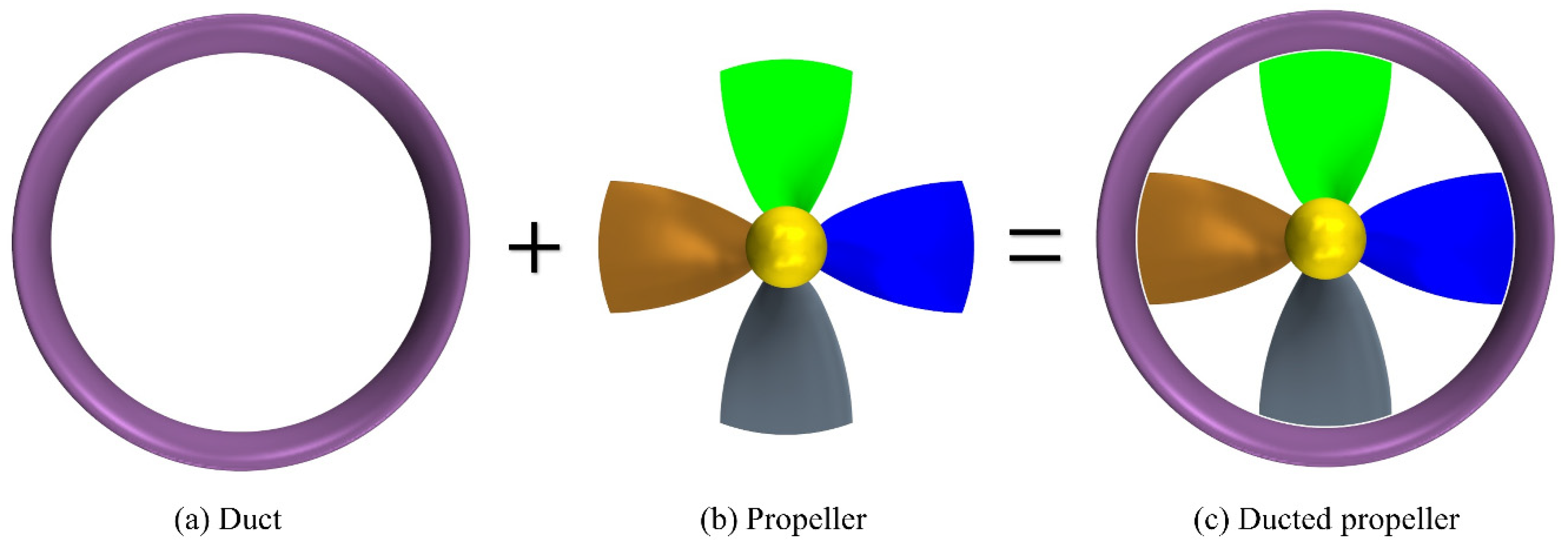
A ducted propeller is composed of a propeller and an annular duct with a two-dimensional hydrofoil in its cross-section. The propeller is fixed in the center of the duct. The duct has a significant optimization effect on the flow field of the propeller and its wake. It can improve the thrust and torque of the propeller, and provides additional thrust under heavy loads and low speeds, thereby significantly improving the propulsion efficiency [1]. In addition, the duct improves the inflow of the propeller [2]; thus, the velocity at the ducted propeller disc surface is much less affected by a change in the ship’s speed than with an ordinary propeller. Therefore, ducted propellers are widely used in the field of ship propulsion.

The hydrodynamic performance of a ducted propeller is affected by many factors. The research on ducted propellers generally involves changing a single parameter to observe its influence on various performance characteristics. Gaggero, Villa, Tani, Viviani, and Bertetta [2] proposed an optimized design method for ducted propeller acceleration ducts and deceleration ducts. Hubless and four pairs of hub-type Ka4-70 propellers with four different hub diameter ratios of 0.05, 0.1, 0.167, and 0.25 were simulated by Song et al. [3]. The simulation results showed that hubless Ka4-70 propellers were more efficient than hub-type Ka4-70 propellers, and the efficiency increased with the increase in the hub diameter and advance coefficient. The numerical analysis of the wake vortex dynamics of ducted and non-ducted propellers was carried out by using the detached eddy simulation (DES) method [4], and the characteristics of the vortex structure under different loading conditions were analyzed in detail. The results showed that the shape and stability of the wake vortex structure of the propeller were significantly affected by the duct. By changing the number of blades, Gong et al. [5] discussed the effect of blade–duct interactions on the wake dynamics. The hydrodynamic characteristics, wake evolution, and instability characteristics of the blades in non-ducted and ducted conditions were also comparatively analyzed.

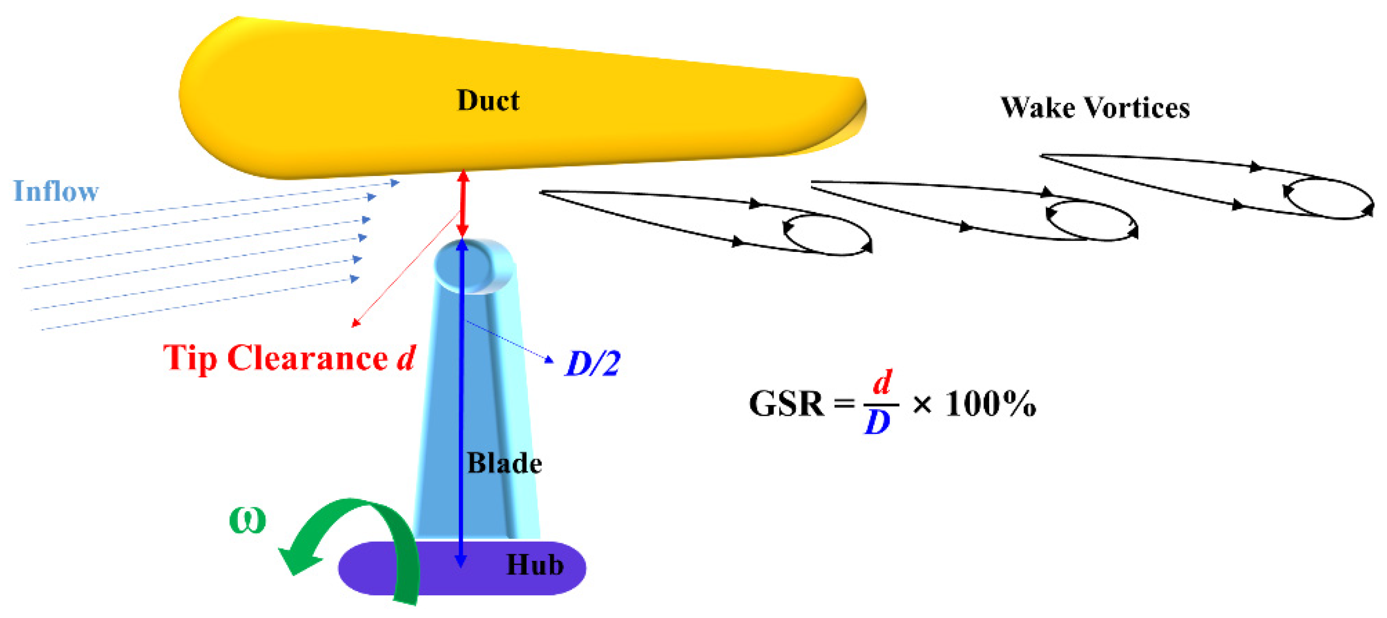
Furthermore, for ducted propellers and other pump machinery, there is a geometric parameter that has a significant influence on the flow field and performance: the tip clearance [6,7]. For a ducted propeller, the flow in its tip clearance area has a significant influence on the performance and the wake, resulting in a special flow phenomenon that is different from that of an ordinary open propeller.

Several simulations on the influence of the tip clearance size showed that the efficiency decreases as the tip clearance increases, and the pressure fluctuation increases with the increase in the tip clearance [8]. Hao et al. [9] studied the energy characteristics and radial forces of symmetric- and asymmetric-tip-clearance mixed-flow pumps, and the results showed that with the increase in the tip clearance, the efficiency decreased. For mixed-flow pumps with asymmetric tip clearance, the energy performance decreased and the total radial force increased. An and Wang [6] used the two-way fluid–structure interaction (FSI) method to analyze the influence of the tip clearance on a composite ducted propeller. However, they did not analyze the influence of the flow field on the propeller’s open-water characteristics (OWCs). The analysis of the ducted propeller vortices, which have a significant effect on the ducted propeller’s wake flow, was also not performed.

Pressure fluctuations and energy recovery are also closely related to the tip clearance, due to differences in the tip leakage vortex (TLV) structure for different values of the tip clearance, and their influence on the wake flow field. The TLV structure of the NACA0009 hydrofoil was studied by Bi et al. [10], and the influence of two types of grooves on the TLV and its suppression mechanism were analyzed. The three-dimensional full-flow field of a pump-jet propeller was simulated based on the DES model by Yuan et al. [11]. The vortex shape of the vortex core in the tip clearance area and the surrounding flow field was obtained by simulations, and the dynamic characteristics of the tip vortex inside the pump-jet propeller were revealed. The important influence of the tip clearance on the pressure fluctuations of the pump and the pump-jet propeller (PJP) was discussed [8,12]. The results showed that with the increase in the tip clearance, the intensity of the leakage vortex enhanced, and the maximum value of pressure fluctuation in the PJP increased significantly. However, the evolution of the TLV was not mentioned in these articles.

In the field of computational fluid dynamics (CFD), the Reynolds-averaged Navier–Stokes (RANS) method [13] has been widely used by many scholars for calculating ducted propellers’ performance [14]. However, the detailed flow fields cannot be captured by the RANS method [15]. Therefore, in recent years, other advanced turbulence models—e.g., the DES model [16], delayed detached eddy simulation (DDES) model, improved delayed detached eddy simulation (IDDES) model, and large eddy simulation (LES) model—have been increasingly used to simulate ducted propellers.

Posa et al. [17] used the LES method to simulate the instability of turbine blade-tip vortex shedding. Jiang et al. [18] developed an LES model of the tip clearance flow of a three-dimensional airfoil with an end-wall moving linear cascade, and discussed the mechanism of the tip clearance vortex variation with respect to tip clearance width. However, the LES method requires a large amount of computation, and it is a huge challenge for current computational resources—especially in the engineering field. By combining the advantages of the RANS and LES models, more accurate simulations can be carried out with limited computational resources, so hybrid RANS–LES models have been widely used in duct machinery in recent years. Zhang and Jaiman [19] used the DDES model and the transient sliding mesh method to perform numerical ducted propeller simulations, and studied the vortex structure evolution and tail loss stability under conditions with zero inflow and different advance coefficients, but the tip clearance effect was not mentioned. A hybrid RANS–LES model was used to study the transient flow of a pre-swirl stator pump-jet propeller by Li et al. [20], and the unsteady forces and wake vortices were compared under the design conditions. The flow of a jet propeller with a pre-swirl pump was numerically simulated using the IDDES method, and the effects of the stator, rotor, and duct on the wake and vortex structures were discussed [21]. However, the influence of the tip clearance size was not taken into consideration by these studies. Liu et al. [22] used numerical methods to study the energy characteristics and TLV of a turbine mixed-flow pump in the pump state, and analyzed the TLV mode, evolution, and related flow instabilities under positive and negative blade rotation angles. However, the interaction relationship between the TLV and the wake dynamics was not explained.

In previous studies, the relationship between the OWCs of ducted propellers and their tip clearance flow has not been clearly elucidated. The evolution of the TLV has rarely been studied. In particular, the mechanism of TLV variation with the size of the tip clearance has not been revealed, nor has the effect of the TLV evolution on the wake stability. Under such circumstances, in this paper, simulations were conducted to study the tip clearance effect on the OWCs and the flow of the ducted propeller, and to reveal the full life-cycle evolution of the TLV under different tip clearance sizes, along with the interaction mechanisms of the wake instability.

This paper is outlined as follows: First, the governing equations and turbulence modeling methods are provided. Then, the geometry of the ducted propeller, its variations, and the OWCs are presented. After that, mesh convergence and the accuracy of the solvers are validated based on five meshes. Finally, simulations of four ducted propellers with different tip clearance sizes by the IDDES method, along with the effect of tip clearance on the OWCs, flow field, and evolution of the TLV, are discussed in detail. Furthermore, fast Fourier transform (FFT) analysis of the pressure and circumferential velocity, along with power spectral density (PSD) analysis at a series of measuring probes in the wake, is presented to explore the effect of the gap-to-span ratio (GSR) on the wake dynamics.

2. Numerical Methods

2.1. Governing Equations

The conservation of fluid mass can be expressed by the following equation, which is also called a continuum equation in CFD:

$$\frac{\partial u_i}{\partial x_i}=0$$

(1)

The fluid is considered to be incompressible. The Navier–Stokes (NS) equations are given as follows:

$$\frac{\partial \left(\rho u_i\right)}{\partial t}+\frac{\partial \left(\rho u_i{u}_j\right)}{\partial x_j}=-\frac{\partial p}{\partial x_i}+\frac{\partial }{\partial x_j}\left[\mu \left(\frac{\partial u_i}{\partial x_j}+\frac{\partial u_j}{\partial x_i}\right)\right]$$

(2)

where ρ is the density, ν is the dynamic viscosity of the fluid, p is the pressure, and u_i and u_j are the velocity components.

2.2. Turbulence Model

The detached eddy simulation (DES) method was employed to calculate the hydrodynamic performance and wake dynamics of ducted propellers with different tip clearances. Considering that the governing equations of the LES and RANS methods are similar, scholars such as Spalart et al. [23] have used the similar mathematical characteristics of the LES and RANS governing equations to adopt a unified governing equation. The momentum equation under incompressible conditions is as follows:

$$\frac{\partial {\tilde{u}}_i}{\partial t}+{\tilde{u}}_j\frac{\partial {\tilde{u}}_i}{\partial x_j}+\frac{1}{\rho }\frac{\partial \tilde{p}}{\partial x_i}=v\frac{{\partial }^2{\tilde{u}}_i}{\partial x_j^2}-\frac{\partial {\tau }_{ij}^{model}}{\partial x_j}$$

(3)

where ${\tau }_{ij}^{model}$ represents the Reynolds stresses in the RANS method, and represents sub-mesh stresses in the LES method. In the hybrid method, ${\tau }_{ij}^{model}$ can be expressed as follows:

$${\tau }_{ij}^{model}=f^{RANS}{\tau }_{ij}^{RANS}+f^{LES}{\tau }_{ij}^{LES}$$

(4)

where $f^{RANS}$ and $f^{LES}$ are the control coefficients of the RANS and LES method changes, respectively.

Compared with the general DES model, the improved delayed DES (IDDES) model introduces a delay function to correct the turbulent characteristic length, thus avoiding the calculation error of the turbulent viscosity in the transition region between the LES and RANS models. In the commercial software Simcenter STAR-CCM+, the IDDES turbulence model that we used is based on the SST k-ω detached eddy model, which combines features of the SST k-ω RANS model in the boundary layers with a large eddy simulation (LES) in unsteady separated regions. The DES formulation of the SST k-ω model is obtained by modifying the dissipation term in the transport equation for the turbulent kinetic energy. The related formulae are expressed as follows [24]:

$$\frac{\partial \left(\rho k\right)}{\partial t}+\frac{\partial \left(\rho u_{j}k\right)}{\partial x_j}=\frac{\partial }{\partial x_j}\left[\left({\mu }_l+{\sigma }_k{\mu }_t\right)\frac{\partial k}{\partial x_j}\right]+{\tau }_{ij}{S}_{ij}-\frac{\rho k^{\frac{3}{2}}}{L_{hybrid}},$$

(5)

$$\frac{\partial \left(\rho \omega \right)}{\partial t}+\frac{\partial \left(\rho u_j\omega \right)}{\partial x_j}=\frac{\partial }{\partial x_j}\left[\left({\mu }_l+{\sigma }_{\omega }{\mu }_t\right)\frac{\partial \omega }{\partial x_j}\right]+\alpha \frac{\omega }{k}{\tau }_{ij}{S}_{ij}-\frac{\rho k^{3/2}}{L_{hybrid}}-\beta \rho {\omega }^2+2\left(1-F_1\right)\frac{\rho {\sigma }_{\omega 2}}{\omega }\frac{\partial k}{\partial x_j}\frac{\partial \omega }{\partial x_j}$$

(6)

where S_ij is the strain tensor, τ_ij is the stress tensor, ρ is the fluid density, ω is the specific dissipation rate, μ_t is the turbulent eddy viscosity, μ_l is the dynamic viscosity, σ_ω2 is a model coefficient, and F₁ is the blending function.

The length scale, L_hybrid, is defined as follows:

$$L_{hybrid}=f_B\left(1+f_e\right)L_{RANS}+\left(1-f_B\right)L_{LES}; L_{RANS}=k^{\frac{1}{2}}/\left({\beta }^{*}\omega \right); L_{LES}=C_{DES}\mathsf{\Delta },$$

(7)

where β * is taken as 0.09 in the k-ω model coefficients, C_DES is specified as 0.78, and Δ is the mesh cell length scale. The elevating function f_e prevents an excessive reduction in the RANS Reynolds stresses, while f_B represents a switching function from the RANS model (f_B = 1) to the LES model (f_B = 0).

3. Geometry and Parametric Study

3.1. Geometric Model

Among the published experimental data of the ducted propeller series, the Ka4-70 propeller in the 19A duct series of the Dutch ship model test pool is the most famous, and is widely used in the marine field. In this study, a four-blade propeller with a disc-to-surface ratio of 0.7 was used, and the pitch ratio P⁄D was selected as 1. The chord length of the blade section at the 0.6R section of the blade was computed according to the following formula:

$$L_{0.6R}=1.969\frac{1}{Z}·\frac{A_E}{A_D}D$$

(8)

where Z is the number of propeller blades, A_E⁄A_D is the disc ratio of the blade, and D is the diameter of the blade. Based on the experimental values described in [25], the diameter D was taken as 218.87 mm, and the tip clearance d was taken as 1.01 mm. The specific parameters of the duct and propeller are presented in detail in

Table 1. Parameters of duct and propeller.

Propeller Model	Ka4-70
Duct Model	19A
Number of blades	Z	4
Diameter	D	0.21887 m
Pitch ratio at 0.7R	P0.7/D	1
Hub diameter ratio	DHUB/D	0.204
Duct length	Lduct	0.5D
Tip clearance	t	1.01 mm

, while the geometric model is shown in Figure 1.

3.2. Parameter Variations

In order to further explore the influence of the tip clearance size on the OWCs of the ducted propeller and the flow characteristics of the wake field, a ducted propeller model with d = 1.01 mm was taken as the standard model, and another four sets of ducted propellers with different tip clearances were added: modified models I, II, III, and IV. Their specific parameters are presented in

Table 2. Parameters of ducted propellers.

Modified Model	Tip Clearance (mm)	Modified Percentage (%)
I	0.5	−50.5
II	1.0	−0.5
III	1.5	+49.5
IV	2.0	+99.5

.

The tip clearance and flow field flow diagrams are shown in Figure 2, and the tip clearance d of the ducted propeller can be expressed by a dimensionless parameter—the GSR, which is defined as follows:

$$GSR=\frac{d}{D}\times 100\%$$

(9)

3.3. Open-Water Characteristics (OWCs)

In the data processing of propeller-related hydrodynamic forces, such as the thrust, torque, and lateral force, the data obtained are dimensionless, so as to obtain the thrust coefficient, thruster efficiency, and torque co-efficiency corresponding to the calculation model. To a certain extent, the dimensionless coefficients are better for visualizing the variation characteristics of the corresponding physical quantities. They have significant influences on open-water propeller tests and CFD simulations. The commonly used performance parameters and formulae of ducted propellers are as follows:

$$J=\frac{V_{in}}{nD}; K_{TB}=\frac{T_B}{\rho n^2{D}^4}; K_{TD}=\frac{T_D}{\rho n^2{D}^4}; K_Q=\frac{Q}{\rho n^2{D}^5}; K_T=K_{TB}+K_{TD},\eta =\frac{J}{2\pi }\frac{K_T}{K_Q},$$

(10)

where V_in represents the inlet velocity of the propeller, K_TB and K_TD are the propeller thrust coefficient and duct thrust coefficient, respectively, K_T is the total thrust coefficient, K_Q is the propeller torque coefficient, η represents the efficiency of the ducted propeller, n is the propeller speed, and D is the propeller diameter.

4. Verification and Validation

4.1. Computational Domain

Based on the experimental setup of Negrato (2015) [25], a rear propeller shaft was adopted to reduce the generation of the hub vortex in the wake and its effect on the wake influence. The calculation area was a hexahedron, and surfaces along the radial direction of the ducted propeller axis (i.e., the positive direction of the x-axis) were taken as squares with side lengths of 9.14D. The distance between the propeller disc surface and the pressure outlet surface was set as 11.42D. The specific values and boundary condition types are shown in Figure 3.

All of the simulations in this paper were performed using Simcenter STAR-CCM + v15.04. This software provides leading computational fluid dynamics capabilities for fast, accurate simulation of complex engineering problems involving fluids, structures, and the associated physics. To verify the accuracy of the numerical computation method, the multiple reference frame (MRF) approach and the IDDES model were employed in the OWC simulation of the standard model. The speed n was set to a fixed value of 15 rps in the standard ducted propeller model simulation. By changing the fluid speed at the inlet—namely, the propeller advance speed V_in—the advance speed coefficient J was changed. The maximum advance speed coefficient was set to 0.8, and the interval was 0.1. Altogether, eight sets of propeller simulations at different advance speeds were carried out. The mesh resolution and calculation steps were appropriately selected to ensure that the calculation results of the simulation at each advance speed reached convergence.

4.2. Mesh Convergence Study

To perform mesh independence analysis, five meshes with different refinement levels were generated, as shown in

Table 3. Parameters for five groups of meshes.

Item (Unit)	M1	M2	M3	M4	M5
Base mesh size (mm)	80	40	20	10	10
Minimum mesh size (mm)	5	2.5	1.25	0.625	0.3125
Target mesh size (mm)	10	5	2.5	1.25	1.25
Total mesh (M)	0.3	0.7	2.4	7.7	10.2

, and the blade mesh diagram with different refinement levels was shown in Figure 4. The MRF approach and the IDDES model were employed for the numerical simulation to obtain the propeller thrust, torque, and duct thrust with J = 0.1–0.8. After non-dimensional processing, the OWC curves of the ducted propeller were obtained.

The numerical simulation of the ducted propeller faces two difficulties that are different from those faced by conventional propellers: the simulation of the flow in the tip clearance area, and the accurate capture of the duct force. The cylinder refinement areas were used in the tip vortex wake area and the duct and tip clearance areas of the ducted propeller to solve these problems. The side mesh view of the entire calculation is shown in Figure 5.

The experimental values of the efficiency η [25] and the η values of the five groups of different mesh resolutions were obtained. Their variations with the advance coefficient were plotted and compared with one another, as shown in Figure 6. The results showed that the simulation results of the efficiency approached the experimental values as the mesh quantity increased, demonstrating that the simulation results were convergent.

A common advance speed coefficient of the Ka4-70 propeller in the 19A duct is 0.6. The simulation results of each mesh resolution with J = 0.6 were analyzed. The simulation results of the ducted propeller’s OWCs approached the experimental values as the mesh resolution increased, and the relative error of each group of simulations also gradually decreased, showing that the simulation results were gradually converging. Thus, the feasibility of the simulation was verified. The blue error bars were used to show the error of the simulated values relative to the experimental values, and the values were marked at the corresponding positions. The errors were all below 5%. Thus, M5 was ultimately selected as the simulation mesh model. The specific convergence results are shown in Figure 7.

4.3. Numerical Validation

Mesh M5 was ultimately used in the simulation. To verify the accuracy of the simulation, the open-water characteristics were compared with the experimental and predicted results obtained by Negrato (2015) [25]. In Figure 8, the experimental values are represented by the dashed lines, while the predicted results achieved by the boundary element method (BEM) and the RANS and BEM mixed method (RANS–BEM) are represented by the black and red points, respectively. The present results show good consistency with the experimental and simulation data from the literature. In particular, the thrust force of the duct, K_TD, is closer to the experimental values. Furthermore, the simulation results of this article are more accurate at J = 0.6, which is the most efficient advance speed coefficient.

The comparison above demonstrated that the simulation results were close to the experimental values, and could gradually converge to the experimental values with the increase in the mesh resolution. This showed that the simulation of the ducted propeller was accurate and effective, verifying the mesh refinement and simulation method described in this paper.

Figure 9 shows the y+ distributions on the ducted propeller. As shown in the picture, the average wall y+ of the duct and the blades is 0.2 and 0.6, respectively. Meanwhile, the y+ near the leading edges on the suction side is relatively higher than that of other areas. It is shown that all y+ values on the ducted propeller faces are well designed, and are generally less than 1.0.

Furthermore, four sets of ducted propeller meshes were generated. The longitudinal section meshes at the tip clearances of the four groups of ducted propellers with different GSRs are shown in Figure 10.

In addition, the simulation method was different in the fine simulation of the four groups of ducted propellers with different tip clearances. In this part of the simulation, in order to improve the simulation accuracy of the flow, the rigid body motion (RBM) method was used instead of the MRF method to simulate the four ducted propellers with GSR = 0.23, 0.46, 0.69, and 0.92. These simulations adopted a transient method, and the time step was set to 1.85 × 10⁻⁵ s. Moreover, for each blade-tip clearance, simulations were carried out with three advance speed coefficients of 0.2, 0.4, and 0.6. Furthermore, simulations of modified models were carried out to reveal the effect of GSR on the OWCs, flow field, TLV evolution, and wake instability.

5. Results and Discussion

5.1. Influence of the Gap-to-Span Ratio (GSR) on OWCs

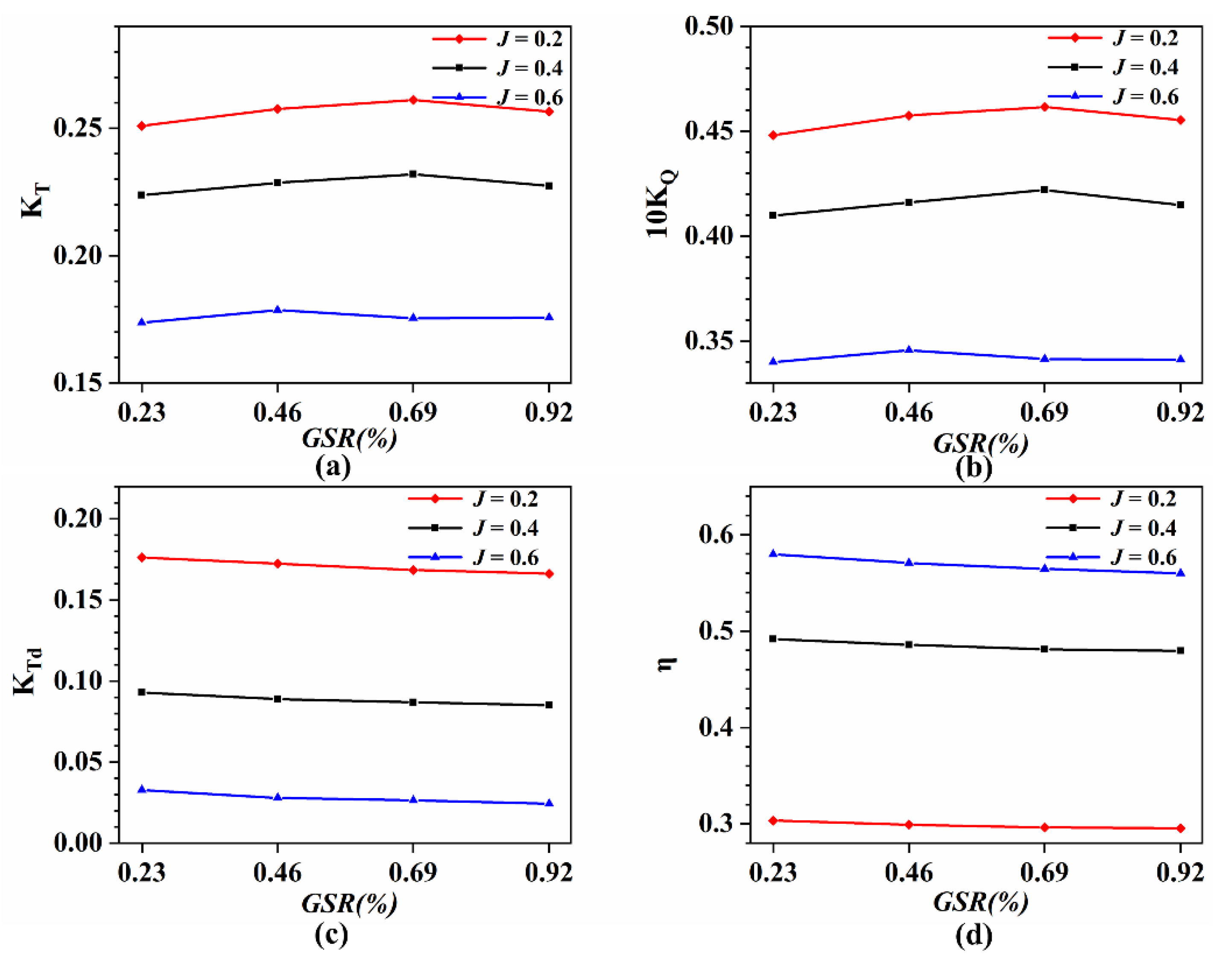
In the numerical simulation, the time history of the blade and duct forces of the ducted propeller was obtained. The calculation was converged after about 1.2 s. Thus, the force and thrust data were derived and averaged within 1.2 s to 1.4 s, which was equivalent to three revolutions of the propeller. After that, the blade thrust, torque, and duct thrust of the ducted propeller were made dimensionless, and the variations of the ducted propeller’s OWCs with the advance speed coefficient and GSR were determined according to the simulation results, as shown in Figure 11. K_TB, K_TD, and the torque coefficient K_Q all decreased as the advance speed coefficient increased, which is consistent with the results shown in Figure 8. With the increase in the GSR, K_Q and K_TB increased, but with a turning point, and an optimal tip clearance d could be achieved. In addition, as the advance coefficient increased, the tip clearance of the ducted blade corresponding to the best thrust and torque of the blade tended to decrease. Moreover, both K_TD and η₀ were gradually reduced.

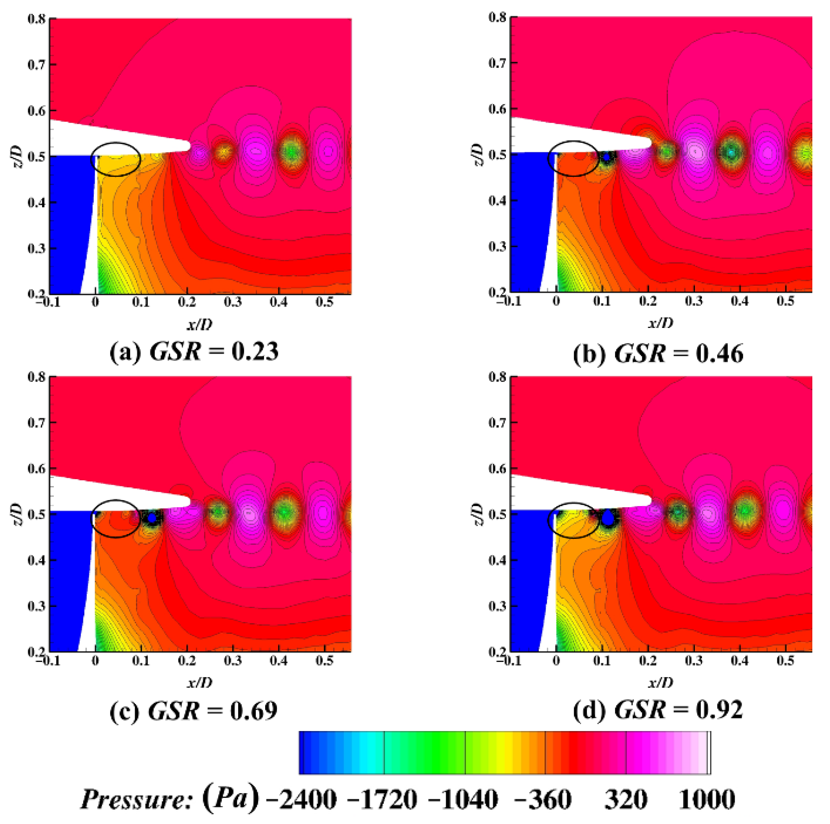
The pressure distribution on the propeller blades and the inner surface of the duct was obtained, as shown in Figure 12. The pressure values marked in black circles in Figure 12a,d were relatively small, while those in Figure 12b,c were relatively high. Since the thrust of propeller comes from the pressure difference between the pressure side and the suction side, when GSR = 0.46 and 0.69, the K_Q and K_TB values related to the blades had a significant increase, while at GSR = 0.92, they reduced instead. Due to the extremely small tip clearance, when GSR = 0.23, the TLV was scattered on the duct surface at a very early stage; thus, no significant vortex shedding area was observed on the inner wall of the duct, while the pressure of areas located in the suction blades of the other three cases was affected by the vortex shedding of the adjacent blades.

It can be concluded that the decrease in both K_Q and K_TB at GSR = 0.92 was mainly due to the mutual influence of the TLV and the duct. The previously occurring large-vorticity area reduced the pressure of the ducted propeller blade’s pressure side, decreasing the hydrodynamic performance coefficients K_Q and K_TB of the propeller.

In fact, the thrust of the ducted propeller is jointly provided by the propeller and the duct, and the vortex leakage of the ducted propeller increases with the increase in GSR, indicating that the total energy loss becomes larger. However, with the decrease in GSR, the interaction between the TLV and the duct becomes stronger, so the thrust force on the duct increases. At this point, the force on the propeller decreases compared with the larger GSR, but the resultant force increases, complying with the conservation of energy.

When referring to the energy recovery of the ducted propeller, we took the combined thrust of the ducted propeller as the output power [26]. The overall energy utilization effect of the ducted propeller increased as the GSR decreased, as can be observed from the efficiency diagram in Figure 11d, showing that the overall efficiency of the ducted propeller decreased with the increase in GSR. That is, the energy recovery of the duct decreased as the GSR increased.

5.2. GSR’s Influence on Tip Leakage Vortex (TLV) Evolution

The TLV of the ducted propeller is its unique flow phenomenon, which has a significant influence on the performance, cavitation, corrosion, and other performance characteristics. Furthermore, it is an extremely important tail vortex structure of the ducted propeller, which has a significant influence on the performance and wake flow instability. Under different GSRs, some differences and similarities in the shapes of the ducted propellers’ TLVs are elaborated.

Since the ducted propeller reached its maximum efficiency near J = 0.6, this advance coefficient was selected to perform numerical simulations on four groups of ducted propellers with different GSRs. The calculations for the four cases reached convergence. Side views of a single-blade vortex are shown in Figure 13. In the TLV evolution process of each ducted propeller, a primary tip leakage vortex (PTLV) and a secondary tip leakage vortex (STLV) were observed. The PTLV occurred near the leading edge of the ducted propeller blade, while the STLV mainly occurred in the middle of the blade, and it developed in clusters at the beginning of its generation. The isosurface of Q = 2 × 10⁵ s⁻² was employed to capture the tip leakage vortex.

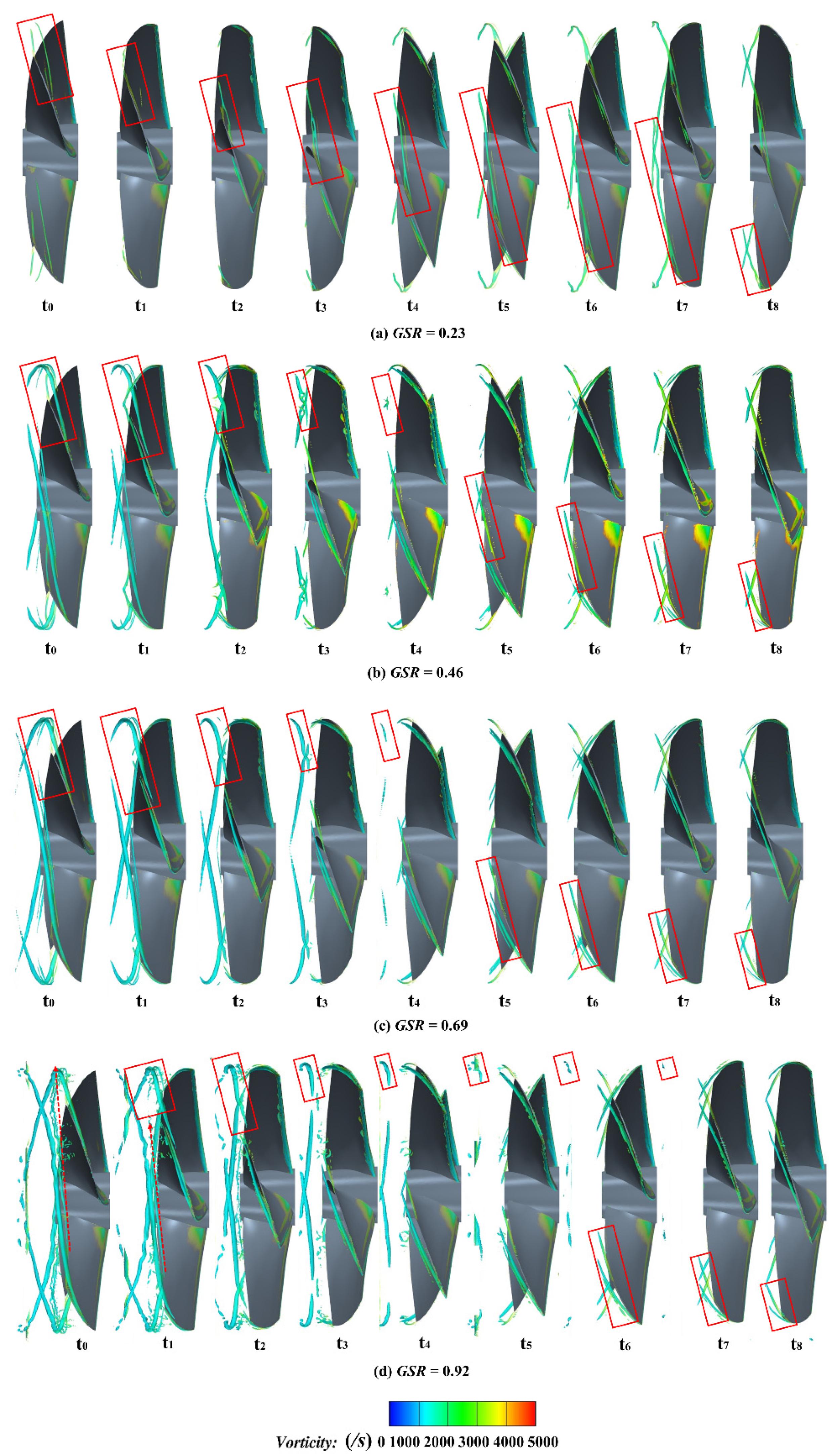
Four groups of ducted propellers with J = 0.6 were simulated to explore the process of TLV generation, development, and evolution. During one revolution, one-third of a rotation period was taken as T. Nine time intervals were averaged to capture the blade vortex leakage at each time node. The TLV in one blade was tracked in nine time intervals to demonstrate the effect of GSR on its generation and evolution process.

Overall, the PTLV was generated at a position slightly closer to the blade’s leading edge, while the STLV was generated at the middle of the blade tip. The STLV merged or collided with the PTLV in its development process, with a significant impact on the stability of the PTLV. The absolute value of the vorticity decreased, while the vortex structure size expanded with the increase in the GSR.

When GSR = 0.23, from the color of the scalar bar, we observed that the vortex value of the vortex structure was larger than that of the other cases, but its extension width was the smallest. At t₀, the vortex was in the attenuation and dissipation stage, and it dissipated completely at time t₁; then, a new cycle of TLV development began. From t₂ to t₅, it was in the development period of the TLV. At t₂ and t₃, the PTLV and STLV merged, and developed together thereafter. At t₅, the development of the TLV effectively reached its maximum. The TLV was in a stable period from t₅ to t₇, and there was no major change in the extended length and stability of the TLV. The stable duration was a special development period when the GSR was small, which was not available in other cases.

At GSR = 0.46 and 0.69, the vortex structures were relatively similar. Both essentially reached the maximum vortex development at time t₀, and then began to attenuate and dissipate from t₂ to t₄. Finally, the vortex structures had mostly dissipated at time t₅, and a new vortex appeared. When the GSR was large—namely, GSR = 0.92 in this simulation—the flow phenomenon was different from the other cases. At t₀, the red arrow indicates that the STLV of the previous blade extended into the vortex system of the next blade and interacted with it. Due to its strong instability, this STLV gradually dissipated at t₁ and t₂, and it completely disappeared at t₃. The influence of the STLV and the instability of the PTLV accelerated the dissipation period relatively quickly. However, its dissipation period was very long (from t₂ to t₆), and the vortex structure of the previous TLV in the upper row of red boxes dissipated very slowly. We speculate that the width and depth of this vortex were larger than those in the other cases.

In summary, the GSR has a significant impact on the ducted propeller’s TLV. With its increase, the TLV structure becomes larger and more complex, and it contains more energy. As a result, less energy is recovered by the ducted propeller, and there is more energy loss in the flow field. Therefore, the GSR of the ducted propeller should be reduced in order to improve the energy recovery effect, which is consistent with the previous analysis of the efficiency. In addition, for the Ka4-70 propeller in the 19A duct, the GSR should be less than 0.9 to avoid the induced merging of the previous blade’s STLV and the incoming blade’s PTLV, as well as to reduce the energy loss of the flow field.

5.3. GSR’s Influence on Wake Instability

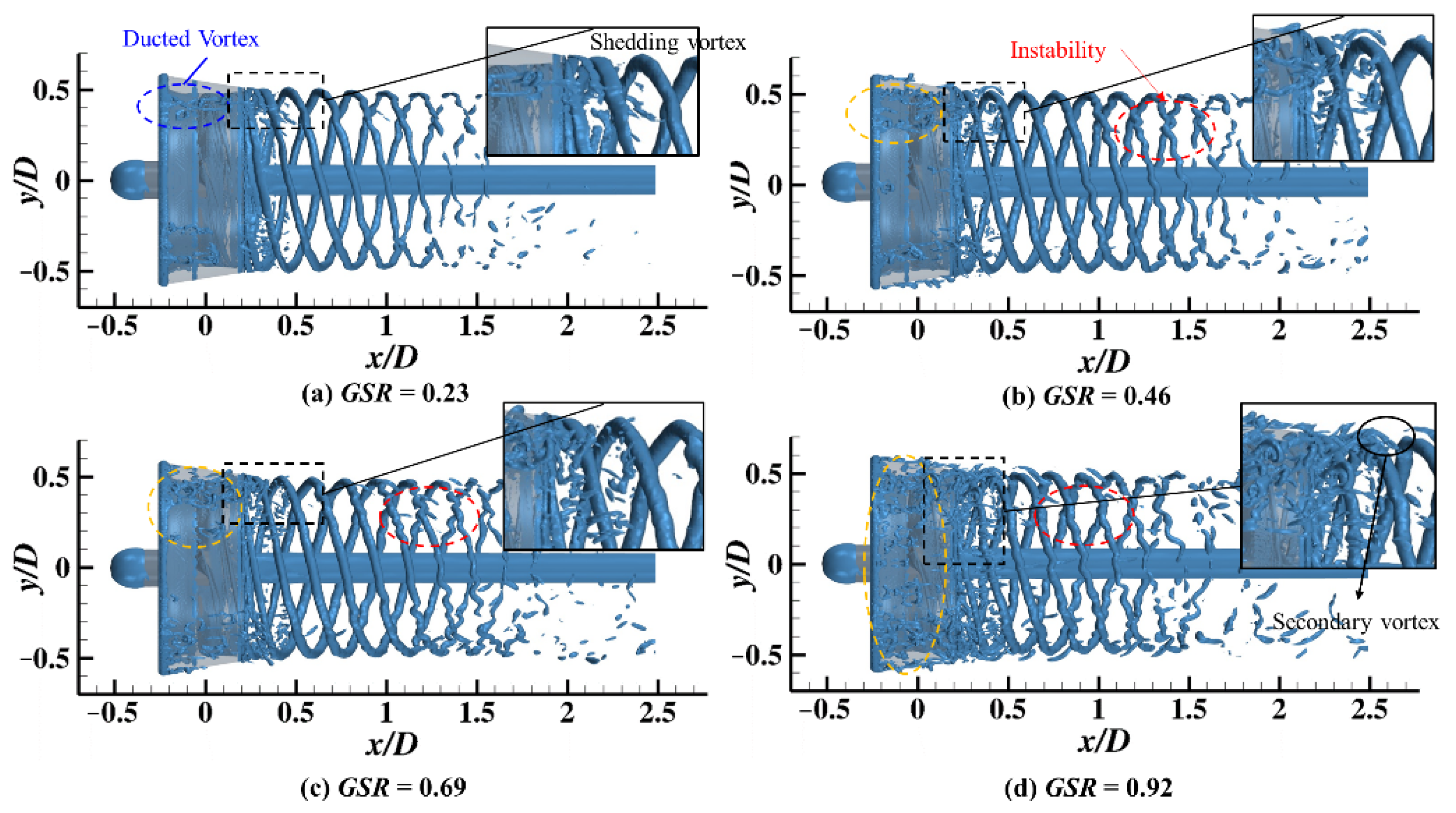
In order to study the effect of the GSR on the evolution and characteristics of the ducted propeller’s wake, the Q = 5000 s⁻² isosurface was employed to capture the tail vortex region of the ducted propeller under different GSRs, and the results were compared. Complex vortex contraction in the ducted propeller wake occurred, as shown by the contours in Figure 14. A duct vortex (DV) on the outer surface of the duct, the PTLV, the STLV, and a duct shedding vortex were produced when the duct vortex met the TLV. Based on the results of the four cases, as the GSR increased, the duct vortex tended to be significantly stronger, and the shedding vortex system became more complicated.

As shown in Figure 14d, there were many duct extension vortices near the PTLV, and as the GSR increased, these vortices extended further. In the evolution of the interaction between the duct extension vortex system and the PTLV, a large number of secondary vortices were generated, whose number and strength increased significantly with the increase in the GSR. Therefore, the wake stability decreased. In particular, as shown in Figure 14a, most of the energy was recovered by the duct because of the narrow tip clearance, and the energy of the TLV was not strong enough, so the TLV extension length was reduced. As shown in Figure 14b–d, the unstable area of the TLV in the wake gradually advanced with the increase in the GSR. The unstable area appeared near x/D = 1.5, 1.2, and 0.9 in Figure 14b–d, respectively. This showed that the instability of the TLV increased as the GSR increased.

The simulation results demonstrated that the unstable region of the TLV in the wake gradually advanced with the increase in the GSR, indicating that the increase in the GSR reduced the stability of the ducted propeller’s wake vortices. The comparative analysis of the four groups of ducted propeller vortices with different GSRs showed that the existence of the STLV was detrimental to the stability of the ducted propeller’s wake, and its strength increased with the increase in the GSR, which affected the stability of the ducted propeller’s wake. However, with the increase in the GSR, the DV increased significantly, which affected the duct extension vortex and weakened the stability of the TLV in the wake.

5.4. GSR’s Influence on Pressure Fluctuations

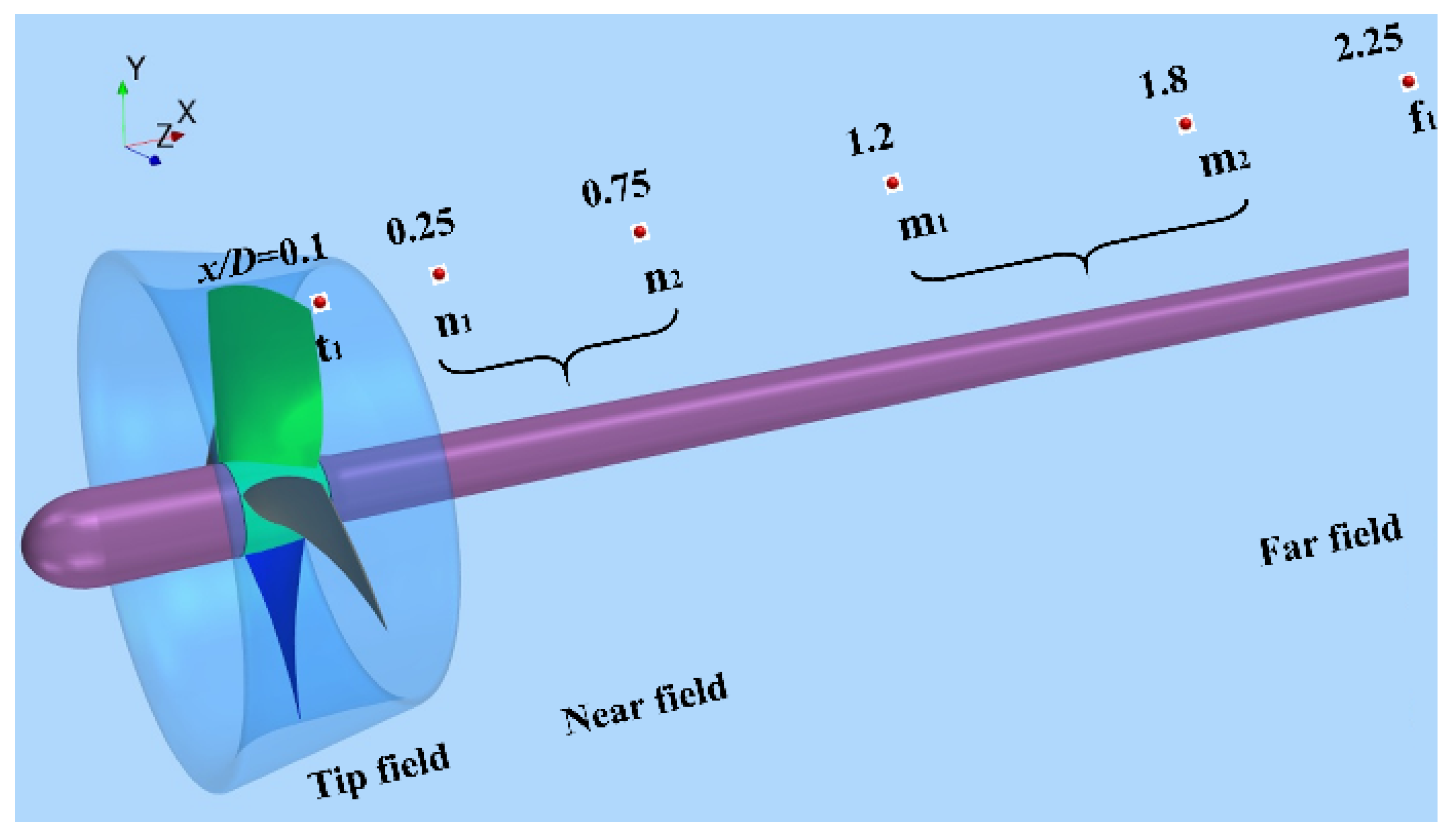
In order to study the effect of the GSR on the dynamic characteristics of the ducted propellers’ wake and the instability of the TLV, when the calculation of the ducted propellers with different GSRs reached convergence—namely, at t = 2 s—six wake detectors located at different positions of the ducted propellers’ wake were selected, and the physical quantity changes of these ducted propellers over three rotation cycles (2–2.2 s) were analyzed. Their longitudinal and circumferential positions were set to be the same—namely, z = 0 and y = 0.9r—and only the axial position changed. The specific locations of the probes are shown in Figure 15, where t₁ is the monitoring point at the blade tip, n₁ and n₂ are the near-field monitoring points, m₁ and m₂ are the mid-field monitoring points, and f₁ is the far-field monitoring point. The pressure p and their frequency-domain distributions were calculated.

As shown in Figure 16, overall, from the tip field to the far-field, the frequency-domain distribution of the pressure measurement points mainly underwent two changes: (1) From the tip area to the near-field, the pressure frequency distribution shifted from nf_b to f_b, (where n = 2,3,4,5…), which was the main blade frequency. It was preliminarily inferred that this was due to the gradual dissipation of the STLV or its interaction with the PTLV. (2) From the near-field to the far-field, the main frequency of the pressure shifted from the main blade frequency to lower frequencies, including 0.5f_b and 0.25f_b, as a consequence of the vortex structure’s evolution in the far-field. Due to the short-wave instability of the TLV, a large number of secondary vortices were generated, and their shedding frequency was irregular.

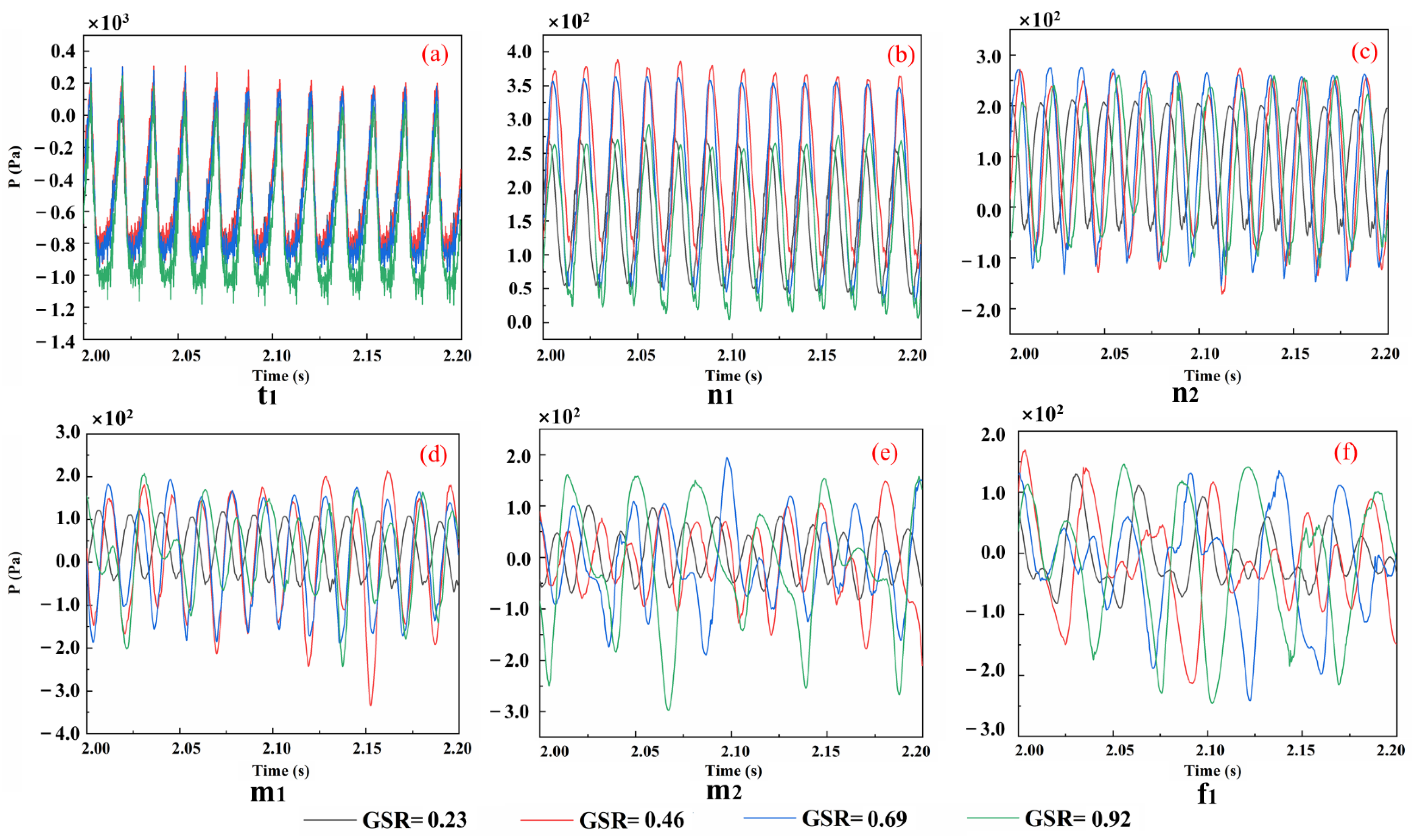
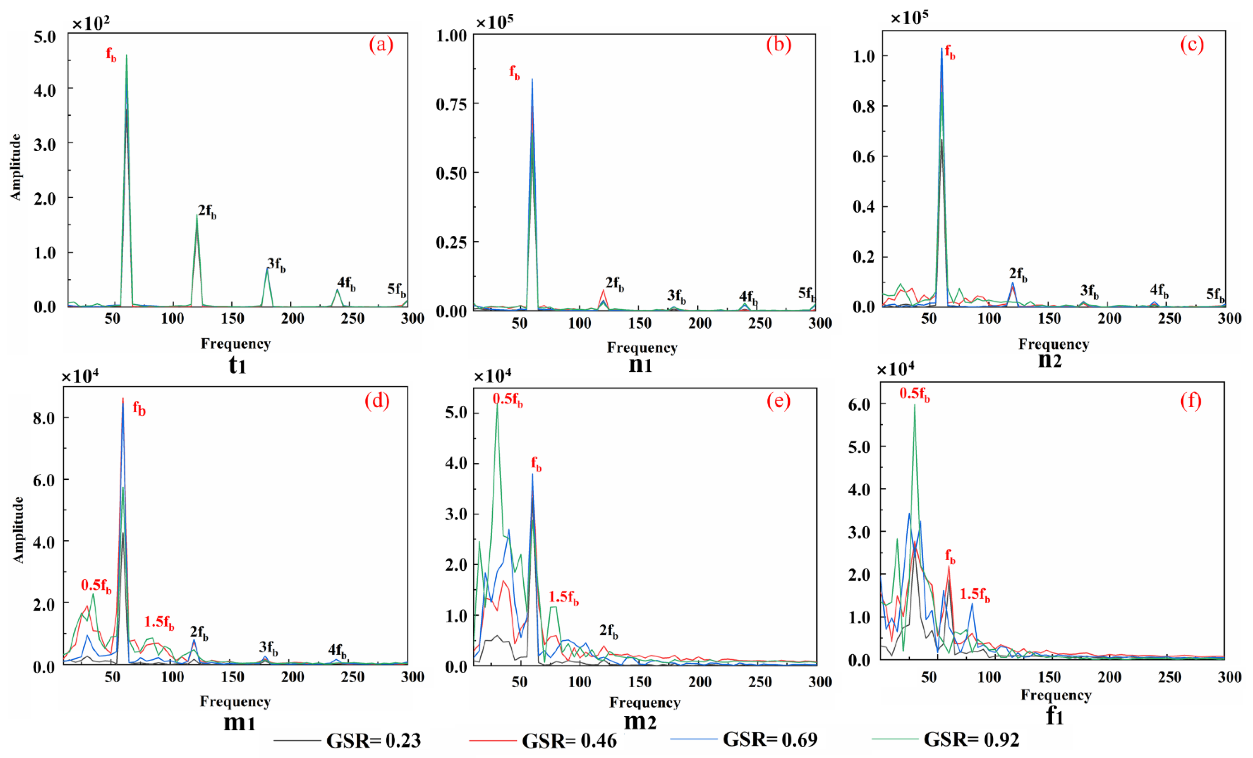
At the tip monitoring point t₁, the GSR’s influence on pressure mainly manifested in its fluctuation amplitude, as shown in Figure 17a. With the increase in the GSR, the pressure fluctuation amplitude gradually increased, indicating that the TLV stability decreased with the increase in the GSR. Overall, a significant peak at nf_b was observed in the pressure spectrum, indicating that the main characteristic frequency of the tip vortex of the ducted blade was the blade-passing frequency. In the near-field, the pressure fluctuation amplitude increased with the increase in the GSR; in the mid-field, while GSR = 0.46 and 0.92, the process of the frequency shifting from f_b to low frequency was more significant; in the mid-field and far-field, with the increase in the GSR, the stability decreased, and the transition area from f_b to the low frequency was advanced. At the same monitoring point, the amplitude of the low blade frequency increased relatively as the GSR increased. When GSR = 0.92, the pressure frequency amplitude had a sharp peak at 0.5f_b, and exceeded the peak values of f_b in m₂ and f₁.

In summary, the evolution of the ducted propeller’s wake in the far-field is mainly the decomposition and dissipation of the TLV, which is caused by the TLV’s instability and the effect of the vortex on the outer edge of the duct. As the GSR increases, the TLV instability increases, and the process of transferring pressure fluctuations of the main blade frequency to the low frequency is accelerated.

5.5. GSR’s Influence on Power Spectral Density

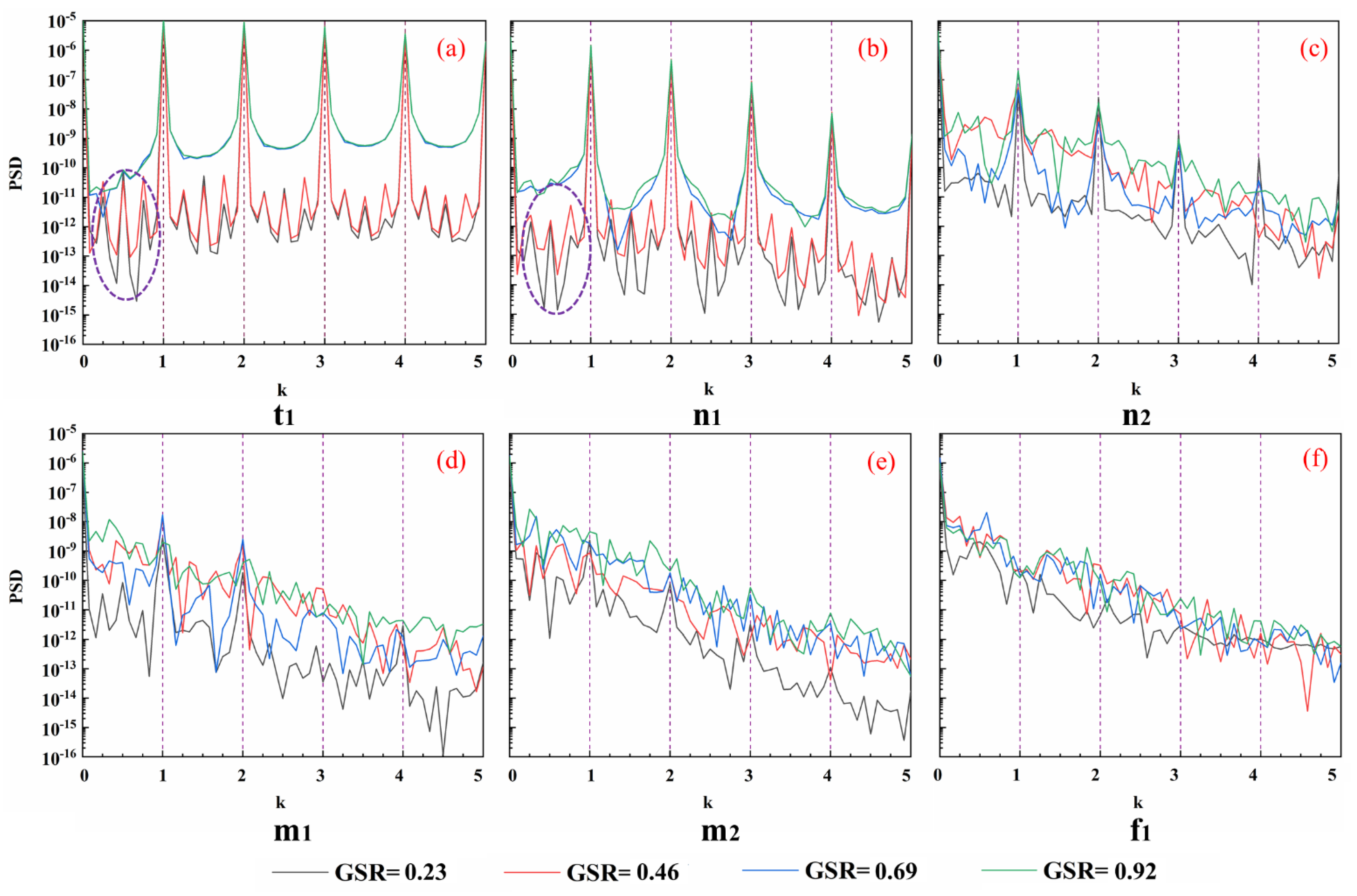
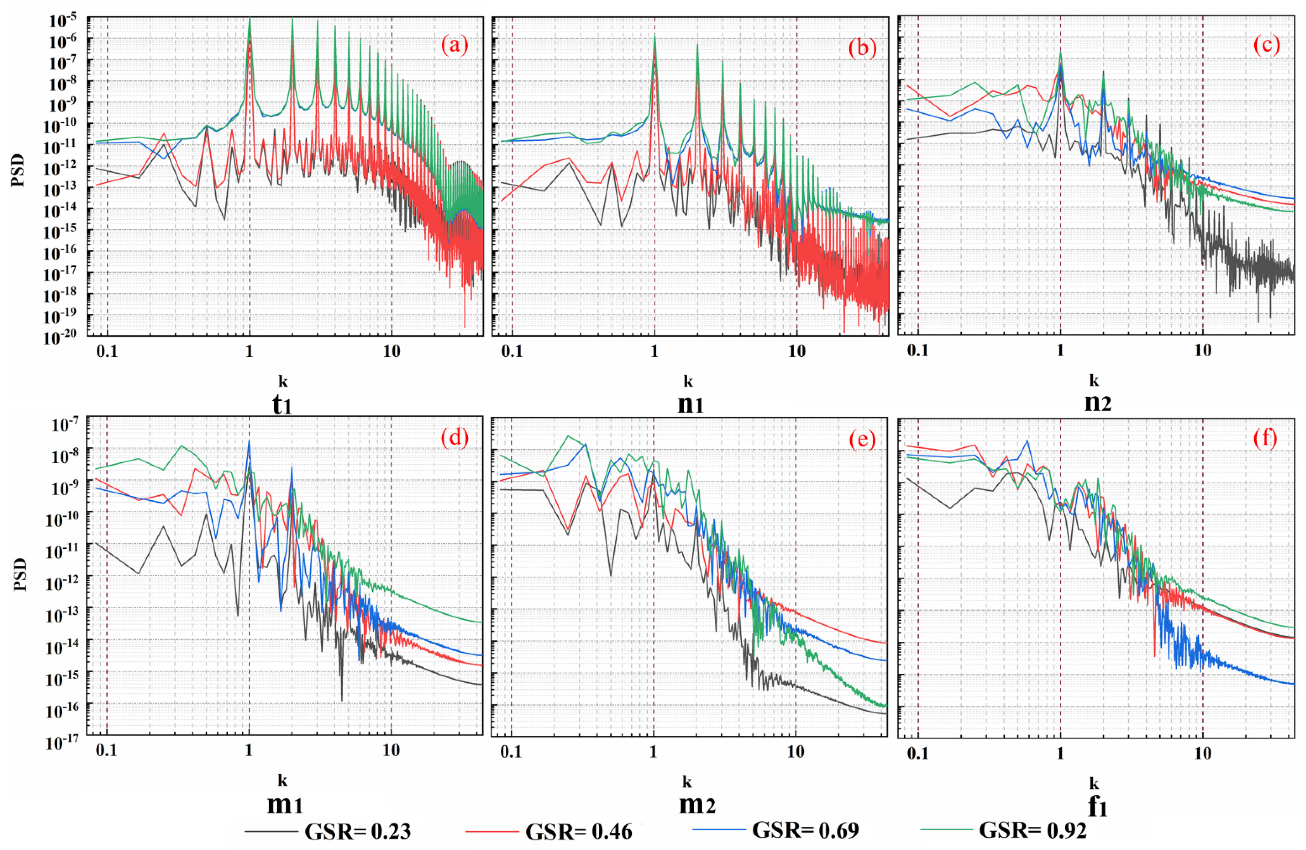
PSD analysis was carried out to determine the GSR’s influence on the energy distribution and the dynamic development of the ducted propeller’s wake.

The PSD distributions followed a similar behavior to the pressure distributions described above, as shown in Figure 18. From the near-field to the mid-field, the PSD distribution frequency spike also gradually shifted from nf_b to f_b, (where n = 2, 3, 4, 5…). In the blade-tip area and the near-field, due to the GSR’s difference, a significant impact on the frequency distribution was observed, as shown in Figure 19a. At t₁, the frequency distribution was divided into two groups: GSR = 0.23, and GSR = 0.46, 0.69, and 0.92. There were significant frequency spikes between the harmonic frequencies of the main leaf frequency when the GSR was small, and when it increased to 0.69 and 0.92 there was no evident spike in the frequency distribution between the harmonic frequencies of the main leaf frequency f_b. The preliminary speculation is that when the GSR of the ducted propeller was small, the effect of the duct extension vortices and the TLV was more significant. In particular, when GSR > 0.5, the interaction was no longer significant, due to the distance relationship.

The horizontal axis was made dimensionless using the blade-passing frequency, which was the main blade frequency, as follows:

$$k=f/f_b$$

(11)

6. Conclusions

In this paper, simulations of modified ducted propeller models were carried out to explore the effect of the GSR on the OWCs, flow field, TLV evolution, and wake instability. Based on the RANS model, the mesh convergence and calculation accuracy were initially verified. Furthermore, the IDDES model and RBM approach were employed to simulate four groups of ducted propellers with different GSRs. Finally, the effects of the GSR on the OWCs, flow field, TLV evolution, and wake instability were revealed. The conclusions based on the simulation results were as follows:

(1)

With the increase in the GSR, K_TD and η₀ gradually decreased, and K_Q and K_TB increased, but with a turning point. At low advance coefficients (J = 0.2 and 0.4), K_Q and K_TB reached maximum values when GSR = 0.69, while at a high advance coefficient of J = 0.6, K_Q and K_TB reached maximum values at GSR = 0.46. Their turning point moved toward the smaller GSR as the advance coefficient increased.

(2)

The energy recovery of the duct was due to the interactions of the TLV and the boundary layer shear vortex on the duct’s inner surface. This effect decreased as the GSR increased, resulting in damage to the energy recovery by the duct. The instability of the wake became worse, and the unstable region moved forward as the GSR increased.

(3)

The FFT of the wake pressure pulsation ranged from high frequency to low frequency, and the evolution process accelerated with the increase in the GSR, indicating that the instability of the wake became worse.

(4)

The energy transfer and recovery of the TLV in the tip area of the ducted propeller were closely related to the GSR. The smaller the GSR, the smaller the energy fluctuation amplitude of the wake field, indicating that more TLV energy was recovered by the duct. However, the PSD analysis at the t₁ measurement point showed that the TLV and duct extension vortex interactions cause significant pressure and turbulent flow energy pulsations in the tip area, which may increase the propeller’s excitation force, as well as having a certain impact on the noise and corrosion performance.

The research of this article will benefit ducted propeller and PJP designers, and help researchers to understand the vortex structure of ducted propellers, as well as energy loss and wake dynamic performance caused by its instability. Future works should be carried out on duct propeller TLV instability and blade-exciting forces. Peculiarly, the effects of the GSR on the OWCs and wake instability of ducted propellers under oblique flow conditions will soon be carried out to approximate the actual operating conditions.

References

1. Park, W.; Jung, Y.; Kim, C. Numerical flow analysis of single-stage ducted marine propulsor. Ocean Eng. 2005, 32, 1260–1277. [Google Scholar] [CrossRef]
2. Gaggero, S.; Villa, D.; Tani, G.; Viviani, M.; Bertetta, D. Design of ducted propeller nozzles through a RANSE-based optimization approach. Ocean Eng. 2017, 145, 444–463. [Google Scholar] [CrossRef]
3. Song, B.; Wang, Y.; Tian, W. Open water performance comparison between hub-type and hubless rim driven thrusters based on CFD method. Ocean Eng. 2015, 103, 55–63. [Google Scholar] [CrossRef]
4. Gong, J.; Guo, C.; Zhao, D.; Wu, T.; Song, K. A comparative DES study of wake vortex evolution for ducted and non-ducted propellers. Ocean Eng. 2018, 160, 78–93. [Google Scholar] [CrossRef]
5. Gong, J.; Ding, J.; Wang, L. Propeller–duct interaction on the wake dynamics of a ducted propeller. Phys. Fluids 2021, 33, 074102. [Google Scholar] [CrossRef]
6. An, X.; Wang, P. Bi-directional fluid-structure interaction for prediction of tip clearance influence on a composite ducted propeller. Ocean Eng. 2020, 208, 107390. [Google Scholar] [CrossRef]
7. Lu, Y.; Wang, X.; Liu, H.; Zhou, F.; Tang, T.; Lai, X. Analysis of the impeller’s tip clearance size on the operating characteristics of the underwater vehicle with a new high-speed water jet propulsion pump. Ocean Eng. 2021, 236, 109524. [Google Scholar] [CrossRef]
8. Liu, Y.; Tan, L.; Hao, Y.; Xu, Y. Energy Performance and Flow Patterns of a Mixed-Flow Pump with Different Tip Clearance Sizes. Energies 2017, 10, 191. [Google Scholar] [CrossRef]
9. Hao, Y.; Tan, L.; Liu, Y.; Xu, Y.; Zhang, J.; Zhu, B. Energy Performance and Radial Force of a Mixed-Flow Pump with Symmetrical and Unsymmetrical Tip Clearances. Energies 2017, 10, 57. [Google Scholar] [CrossRef] [Green Version]
10. Bi, Z.; Zhang, L.; Shao, X. Numerical study of suppression mechanism of two types of grooves on the TLV. Ocean Eng. 2021, 224, 108637. [Google Scholar] [CrossRef]
11. Yuan, J.; Chen, Y.; Wang, L.; Fu, Y.; Zhou, Y.; Xu, J.; Lu, R. Dynamic Analysis of Cavitation Tip Vortex of Pump-Jet Propeller Based on DES. Appl. Sci. 2020, 10, 5998. [Google Scholar] [CrossRef]
12. Yu, H.; Zhang, Z.; Hua, H. Numerical investigation of tip clearance effects on propulsion performance and pressure fluctuation of a pump-jet propulsor. Ocean Eng. 2019, 192, 106500. [Google Scholar] [CrossRef]
13. Martio, J.; SánchezCaja, A.; Siikonen, T. Open and ducted propeller virtual mass and damping coefficients by URANS-method in straight and oblique flow. Ocean Eng. 2017, 130, 92–102. [Google Scholar] [CrossRef]
14. Bhattacharyya, A.; Krasilnikov, V.; Steen, S. A CFD-based scaling approach for ducted propellers. Ocean Eng. 2016, 123, 116–130. [Google Scholar] [CrossRef]
15. Stark, C.; Shi, W. The influence of leading-edge tubercles on the hydrodynamic performance and propeller wake flow development of a ducted propeller. In Proceedings of the 31st International Ocean and Polar Engineering Conference, Rhodes, Greece, 20–25 June 2021. [Google Scholar]
16. Cao, L.; Huang, F.; Liu, C.; Wan, D. Vortical structures and wakes of a sphere in homogeneous and density stratified fluid. J. Hydrodyn. 2021, 33, 207–215. [Google Scholar] [CrossRef]
17. Posa, A.; Broglia, R.; Balaras, E. Instability of the tip vortices shed by an axial-flow turbine in uniform flow. J. Fluid Mech. 2021, 920, A19. [Google Scholar] [CrossRef]
18. Jiang, J.; Wang, W.; Chen, K.; Huang, W. Large-eddy simulation of three-dimensional aerofoil tip-gap flow. Ocean Eng. 2022, 243, 110315. [Google Scholar] [CrossRef]
19. Zhang, Q.; Jaiman, R.K. Numerical analysis on the wake dynamics of a ducted propeller. Ocean Eng. 2019, 171, 202–224. [Google Scholar] [CrossRef]
20. Li, H.; Huang, Q.; Pan, G.; Dong, X. The transient prediction of a pre-swirl stator pump-jet propulsor and a comparative study of hybrid RANS/LES simulations on the wake vortices. Ocean Eng. 2020, 203, 107224. [Google Scholar] [CrossRef]
21. Qin, D.; Huang, Q.; Pan, G.; Shi, Y.; Han, P.; Dong, X. Effect of the duct and the pre-swirl stator on the wake dynamics of a pre-swirl pumpjet propulsor. Ocean Eng. 2021, 237, 109620. [Google Scholar] [CrossRef]
22. Liu, Y.; Han, Y.; Tan, L.; Wang, Y. Blade rotation angle on energy performance and tip leakage vortex in a mixed flow pump as turbine at pump mode. Energy 2020, 206, 118084. [Google Scholar] [CrossRef]
23. Spalart, P.R.; Deck, S.; Shur, M.L.; Squires, K.D.; Strelets, M.K.; Travin, A. A New Version of Detached-eddy Simulation, Resistant to Ambiguous Grid Densities. Theor. Comput. Fluid Dyn. 2006, 20, 181–195. [Google Scholar] [CrossRef]
24. Shur, M.L.; Spalart, P.R.; Strelets, M.K.; Travin, A.K. A hybrid RANS-LES approach with delayed-DES and wall-modelled LES capabilities. Int. J. Heat Fluid Flow 2008, 29, 1638–1649. [Google Scholar] [CrossRef]
25. Negrato, C. Prediction of the Performance of Ducted Propellers with BEM and Hybrid RANS-BEM Methods. Master’s Thesis, Delft University of Technology, Delft, The Netherlands, 2015. [Google Scholar]
26. Zhang, X.; Wu, J.; Cao, L.; Wan, D. Comparative study on wake instabilities of a propeller with and without duct. In Proceedings of the Thirty-Second (2022) International Ocean and Polar Engineering Conference, Shanghai, China, 5–10 June 2022. [Google Scholar]
Figure 1. Geometric model of the Ka4-70 propeller in the 19A duct.
Jmse 10 01007 g001
Figure 2. Schematic diagram of the ducted propeller’s flow field.
Jmse 10 01007 g002
Figure 3. Specific values and boundary condition types of the ducted propeller.
Jmse 10 01007 g003
Figure 4. Five groups of propeller blade surface meshes.
Jmse 10 01007 g004
Figure 5. Side mesh view of the entire calculation.
Jmse 10 01007 g005
Figure 6. Comparison of the experimental and simulated values of the efficiency η.
Jmse 10 01007 g006
Figure 7. Open-water performance simulation results and error percentages with experimental values: (a) Change of KT with mesh number; (b) Change of 10KQ with mesh number; (c) Change of KTD with mesh number; (d) Change of η with mesh number.
Jmse 10 01007 g007
Figure 8. Open-water performance simulation results and comparison with literature [25] values.
Jmse 10 01007 g008
Figure 9. Wall y+ of the ducted propeller when J = 0.6.
Jmse 10 01007 g009
Figure 10. Side views of the meshes of propellers with different gap-to-span ratios (GSRs).
Jmse 10 01007 g010
Figure 11. (a) Change of KT with GSR; (b) Change of 10KQ with GSR; (c) Change of KTD with GSR; (d) Change of η with GSR.
Jmse 10 01007 g011
Figure 12. Side view of pressure near the tip clearance of four groups of ducted propellers with different GSRs.
Jmse 10 01007 g012
Figure 13. Generation and evolution process of tip leakage vortices (TLVs) of four ducted propellers.
Jmse 10 01007 g013
Figure 14. Result comparison of the tail vortex region of the ducted propeller with different GSRs.
Jmse 10 01007 g014
Figure 15. Layout of the wake measuring points.
Jmse 10 01007 g015
Figure 16. Diagram of pressure–time changes at the measuring points: (a) The time history of pressure at t1 measuring point; (b) The time history of pressure at n1 measuring point; (c) The time history of pressure at n2 measuring point; (d) The time history of pressure at m1 measuring point; (e) The time history of pressure at m2 measuring point; (f) The time history of pressure at f1 measuring point.
Jmse 10 01007 g016
Figure 17. Diagram of pressure–frequency changes at the measuring points: (a) The frequency distribution of pressure at t1 measuring point; (b) The frequency distribution of pressure at n1 measuring point; (c) The frequency distribution of pressure at n2 measuring point; (d) The frequency distribution of pressure at m1 measuring point; (e) The frequency distribution of pressure at m2 measuring point; (f) The frequency distribution of pressure at f1 measuring point.
Jmse 10 01007 g017
Figure 18. Diagram of power spectral density (PSD) at the measuring points: (a) The PSD distribution at t1 measuring point; (b) The PSD distribution at n1 measuring point; (c) The PSD distribution at n2 measuring point; (d) The PSD distribution at m1 measuring point; (e) The PSD distribution at m2 measuring point; (f) The PSD distribution at f1 measuring point.
Jmse 10 01007 g018
Figure 19. Enlarged diagram of PSD at measuring points. (a) The PSD distribution at t1 measuring point; (b) The PSD distribution at n1 measuring point; (c) The PSD distribution at n2 measuring point; (d) The PSD distribution at m1 measuring point; (e) The PSD distribution at m2 measuring point; (f) The PSD distribution at f1 measuring point.
Jmse 10 01007 g019