Numerical Investigation of Internal Solitary Wave Forces on a Moving Submarine

Abstract

A numerical model is developed to investigate the hydrodynamic characteristics of a moving submarine induced by internal solitary waves (ISWs) in continuously stratified fluids. A new numerical scheme for the generation of ISWs with a current is proposed, in which the forward speed of the submarine is equivalent to the current. The superposition of the velocity field obtained from extended Korteweg-de Vires (eKdV) theory and the velocity field of the current is taken as the initial velocity field in a numerical wave tank. Convergence analysis is conducted, while the present numerical model is validated by comparing it with experimental data. Then, the interaction between the moving submarine and the ISWs against different pycnocline thicknesses and different moving speeds is investigated. The proposed numerical model can produce accurate ISWs coupled with a current. It can be found that the hydrodynamic forces on the submarine decrease with the increment of pycnocline thickness. The moving speed of the submarine performs a significant effect on the horizontal force, but a light effect on the vertical forces and the torque. It is also found that the forces on the moving submarine cannot be considered as the linear superposition of the navigation resistance in still water and the forces induced by ISWs.

1. Introduction

The internal solitary wave is a kind of strong nonlinear wave with a large amplitude that often appears in the stratified ocean. The balance between dispersion and nonlinearity leads to the propagation of ISWs with a stable waveform and propagation speed in the ocean. ISWs carry enormous energy and the propagation of ISWs can induce strong convergence and divergence. Thus, ISWs can enhance the mixing of deep water and surface water because of strong vertical shear force and wave breaking, which have an important impact on the ecological environment of the ocean [1].

ISWs are potential threats to ocean structures, especially platforms and submarines. As the platform is usually moored to a particular sea area for operation, it is difficult to avoid the extreme sea environment. Therefore, the loads on the platform induced by the ISWs cannot be negligible [2]. The interaction problem between the platform and the ISWs has been numerically and experimentally studied by many researchers. A time-domain numerical model was established by Song et al. [3] to compute the evolution of ISWs and the structure motion responses. It was found that the motion response due to ISWs is much greater than the one due to surface waves. To further explore the interaction mechanism between platforms and ISWs Wang et al. [4,5] conducted a series of laboratory experiments and numerical tests to investigate the ISW loads on a semi-submersible platform. The results indicated that the horizontal and vertical forces on the semi-submersible platform due to ISWs can be divided into three components, namely the wave pressure-difference force, viscous pressure-difference force, and the frictional force, in which the frictional force is negligible. The experiments conducted by Chen et al. [6] and the numerical simulation performed by Ding et al. [7] indicated that the maximums of the forces and moments increase linearly with ISW amplitude and layer depth.

Except for the platforms, submarines are in more danger when they encounter ISWs since submarines can be dragged into the deep sea and crushed violently [8,9]. Fu et al. [10] numerically simulated ISW interaction with a submarine at different depths and calculated the ISW loads on the submarine. The speed of the submarine was neglected in Fu’s research. To investigate the influence of the submarine speed, Chen et al. [11] developed an ISW numerical wave tank by velocity inlet and open-channel flow methods. The ISW-induced forces on the moving submarine were numerically simulated. The motion-response characteristics of the submarine encountering ISWs are also important. Huang et al. [12] investigated the motion response of the SUBOFF under the action of ISWs. It indicated that the flow fields become very complex when a submarine goes through solitary waves, resulting in extremely considerable loads and motion.

In most of these studies, the stratified fluid was simply regarded as a two-layer system, however, the density of the stratified fluids in the actual ocean is continuous and miscible. Li et al. [13] developed a numerical model of ISWs in continuously stratified fluids by introducing a density transport equation to the three-dimensional Navier-Stokes equation. The model was then used to numerically analyze the forces and moments of the standard submarine model encountering ISWs at different depths. But the speed of the submarine in Li’s simulation was neglected. It is significant to investigate the interaction between the ISWs and moving submarines in continuously stratified fluids. The key in the simulation of a moving submarine interaction with ISWs is how to simulate the submarine speed. Generally, there are two numerical technologies that can simulate a moving submarine. One is the dynamic mesh method; however, it requires a lot of high-cost computing resources [12]. Another one is substituting the submarine speed with a current, which is adopted in this study. Chen et al. [11] applied the velocity inlet method to generate ISWs. Firstly, the ISWs were generated by giving the velocity of the upper layer and lower layer at the inlet, where the velocity was calculated by ISW theory. Then, the velocity at the inlet was changed to constant when the waveform of ISW was stable. However, in this method, the velocity of the current can influence the waveform of ISWs, which leads to numerical errors.

This research aims to simulate more stable internal solitary waves with a current by optimizing the initial condition. In this research, the velocity fields of the fluids were derived from eKdV and the submarine speed. The above solutions were applied to initialize the flow field in a numerical wave tank based on the open-source code, Open Field Operation and Manipulation (OpenFOAM), and the third-party software packages ISWFoam [14]. Using the proposed numerical method, the interaction of ISWs and the moving submarine was studied. Firstly, the proposed numerical model was validated by experimental data. Then, a series of ISWs were generated using the established wave tank. The velocity fields and the wave profiles in the propagation of the ISWs were investigated. Next, the interaction between the moving submarine and the ISWs against different pycnocline thicknesses was investigated. It was found that as the pycnocline thickness increases, the hydrodynamic force on the submarine decreases. Finally, the interaction between the moving submarine and the ISWs against different moving speeds was investigated. The moving speed of the submarine performs more significant effects on the horizontal force than the vertical forces and the torque. It was also found that the forces on a moving submarine cannot be regarded as a linear superposition of the navigation resistance in still water and the ISW-induced forces.

2. Numerical Model

2.1. Governing Equations

The governing equations are the mass continuity equation and the Reynolds Average Navier-Stokes (RANS) equation. They can be written as follows [15,16]:

$$\nabla \cdot \mathbf{U}=0,$$

(1)

$$\frac{\partial U}{\partial t}+\nabla \cdot (\mathbf{U}\mathbf{U})-\nabla (\upsilon \nabla \mathbf{U})=-\frac{1}{\rho }\nabla p_{rgh}-g\cdot X\nabla \rho ,$$

(2)

where U = (u₁, u₂, u₃) is the velocity vector of the fluid particles; t is the time; υ is the kinetic viscosity; ρ is the density; p_rgh is the modified pressure; g is the gravitational vector; X = (x, y, z) is the position vector.

In the actual oceans, the density of fluids is stratified continuously, and fluids with different densities are miscible. In this study, a density transport equation is introduced to describe the advection–diffusion process between fluids with different densities. The density transport equation can be written as follows:

$$\frac{\partial \rho }{\partial t}+\nabla \cdot (\rho \mathbf{U})=\nabla \cdot (D\nabla \rho ),$$

(3)

where D is the diffusion coefficient, and its value is the same as the kinetic viscosity.

To close the above equation system, the turbulent viscosity needs to be solved by the turbulence model. The most popular turbulence models are the k-ω and the k-ε models. The k-ε model is widely used to study the propagation of ISWs and the resistance of submarines. For example, Liu et al. [17] used realizable k-ε to solve the turbulence when studying the resistance and flow field of a submarine in a density stratified fluid. Hsieh et al. [18] used the k-ε model to study the propagation of ISWs. However, the k-ε model is not suitable for the low Reynolds number conditions; it cannot reflect the flow in the boundary layers properly because of the adverse pressure gradients [19]. Therefore, Huang et al. [20] and Menter et al. [21] suggested using the SST k-ω model to obtain more accurate results, which is adopted in this research.

The advection–diffusion equation for k is given as:

$$\frac{\partial \rho k}{\partial t}+\nabla (\rho \mathbf{U}k)=\nabla \left[\rho \left(\upsilon +{\sigma }_k{\upsilon }_t\right)\nabla k\right]+P_k^{*}-{\beta }^{*}\omega k,$$

(4)

ω can be derived from:

$$\frac{\partial \rho \omega }{\partial t}+\nabla \cdot (\rho \mathbf{U}\omega )=\nabla \cdot \left[\rho \left(\upsilon +{\sigma }_{\omega }{\upsilon }_t\right)\nabla \omega \right]+\rho \left[C_{\gamma }\frac{\omega }{k}{P}_k-C_{\beta }{\omega }^2+2(1-F_1)\frac{{\sigma }_{{\omega }^2}}{\omega }\nabla k\cdot \nabla \omega \right],$$

(5)

where:

$${\upsilon }_t=\frac{a_{1}k}{\max (a_1\omega ,\sqrt{2}{S}_t{F}_2)},$$

(6)

$$P_k={\tau }^R:\nabla \mathbf{U},$$

(7)

$$P_k^{*}=\min (P_k,c_1{C}_{\mu }k\omega ),$$

(8)

$$S_t=0.5(\nabla \mathbf{U}+\nabla {\mathbf{U}}^T)$$

(9)

The coefficients in the expressions take the following values: β* = 0.09, a₁ = 0.31, c₁ = 10, C_μ = 0.09.

The governing equations are numerically solved by the finite volume method. Time advancement is performed by the implicit Euler method. The velocity gradient on the left-hand side of Equation (1) is obtained by the Gaussian linear interpolation. The pressure-velocity coupling term is solved by using the PIMPLE algorithm, which is a combination of the pressure implicit with the splitting of operator (PISO) algorithm and the semi-implicit method for pressure-linked equations (SIMPLE) algorithm. PIMPLE algorithm allows for equations under relaxation to ensure the convergence at each time step. More details of the PIMPLE algorithm can be found in Jasak [22].

2.2. ISW Generation

Different ISW theories are suitable for different depth ratios β = h₁/h₂ and amplitude parameters α = a/H. The ISWs generated by eKdV theory are in good agreement with experimental data when α > 0.1 [23]; therefore, the eKdV theory is adopted to initialize the ISW fields in this research. The interface displacement of the eKdV equation can be written as follows:

$$\frac{\partial \zeta }{\partial t}+c_0\frac{\partial \zeta }{\partial x}+c_1\zeta \frac{\partial \zeta }{\partial x}+c_2\frac{{\partial }^3\zeta }{\partial x^3}+c_3{\zeta }^2\frac{\partial \zeta }{\partial x}=0$$

(10)

$$c_0{}^2=\frac{g{h}_1{h}_2({\rho }_2-{\rho }_1)}{{\rho }_1{h}_2+{\rho }_2{h}_1}$$

(11)

$$c_1=\frac{-3c_0({\rho }_1{h}_2{}^2-{\rho }_2{h}_1{}^2)}{2({\rho }_1{h}_1{h}_2{}^2+{\rho }_2{h}_1{}^2{h}_2)}$$

(12)

$$c_2=\frac{c_0({\rho }_2{h}_1{h}_2{}^2+{\rho }_1{h}_1{}^2{h}_2)}{6({\rho }_1{h}_2+{\rho }_2{h}_1)}$$

(13)

$$c_3=\frac{3c_0}{h_1{}^2{h}_2{}^2}\left[\frac{7}{8}{\left(\frac{{\rho }_1{h}_2{}^2-{\rho }_2{h}_1{}^2}{{\rho }_1{h}_{{}^2}+{\rho }_2{h}_1}\right)}^2-\left(\frac{{\rho }_1{h}_2{}^3+{\rho }_2{h}_1{}^3}{{\rho }_1{h}_2+{\rho }_2{h}_1}\right)\right]$$

(14)

where ζ denotes the ISW wave profile; ρ₁ and ρ₂ are the density of the upper layer and lower layer respectively; h₁ and h₂ are the depth of the upper layer and the lower layer, respectively.

The analytical solution of ζ is:

$$\varsigma =\frac{a}{B+(1-B){\cosh }^2\left[{\lambda }_{\mathrm{eKdV}}(x-c_{\mathrm{eKdV}}t)\right]}$$

(15)

$${\lambda }_{\mathrm{eKdV}}=\sqrt{\frac{a}{12c_2}\left(c_1+\frac{1}{2}{c}_{3}a\right)}$$

(16)

$$c_{\mathrm{eKdV}}=c_0+\frac{a}{3}(c_1+\frac{c_{3}a}{2})$$

(17)

$$B=\frac{-a{c}_3}{2c_1+a{c}_3}$$

(18)

where a is the wave amplitude; λ_eKdv is the wavelength; c_eKdv is the eKdV theory phase velocity; B is an auxiliary parameter.

The upper layer and lower layer velocity can be derived from the ISW profiles respectively. u₀ is the velocity of the current.

$$u_1=-c_{\mathrm{eKdV}}\frac{\varsigma }{h_1-\varsigma }+u_0$$

(19)

$$u_2=c_{\mathrm{eKdV}}\frac{\varsigma }{h_1+\varsigma }+u_0$$

(20)

The density profile is given by a hyperbolic tangent function profile [24], the initial density distribution can be expressed as follows:

$$\left\{\begin{array}{l}{\rho }_1\\ \frac{{\rho }_1+{\rho }_2}{2}\left\{1-\frac{{\rho }_2-{\rho }_1}{{\rho }_1+{\rho }_2}\tanh \left(\frac{z-z_c}{d_c}\right)\right\}\\ {\rho }_3\end{array}\right.\begin{array}{l}(z>z_c+\frac{d_c}{2})\\ (z_c-\frac{d_c}{2}<z<z_c+\frac{d_c}{2})\\ (z<z_c-\frac{d_c}{2})\end{array}$$

(21)

where z is the vertical position; z_c is the vertical location of the pycnocline center. The pycnocline center is obtained by calculating the gradient of the density field. The maximum value of the gradient represents the position of the center of the pycnocline. d_c is the thickness of the pycnocline.

3. Model Verification

The hydrodynamic problem of a submarine navigating in single-layer fluid was investigated to validate the proposed numerical model. First, the arrangement of the computational domain and the mesh technologies adopted in this research were introduced. Then, the convergence analysis was conducted. Next, the calculated resistance of the submarine was compared with the experimental data.

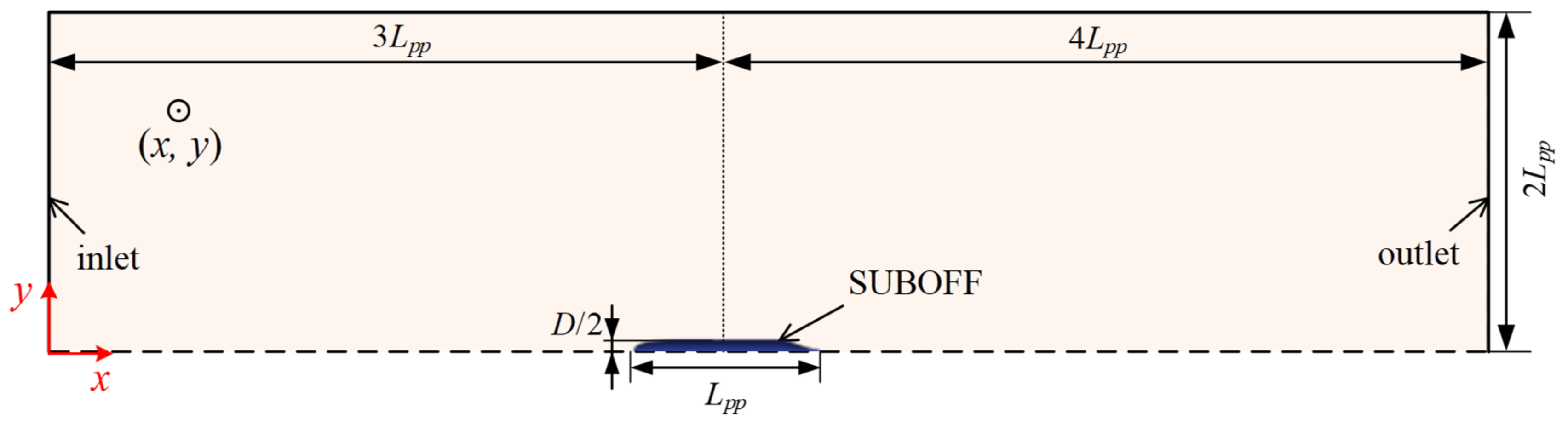
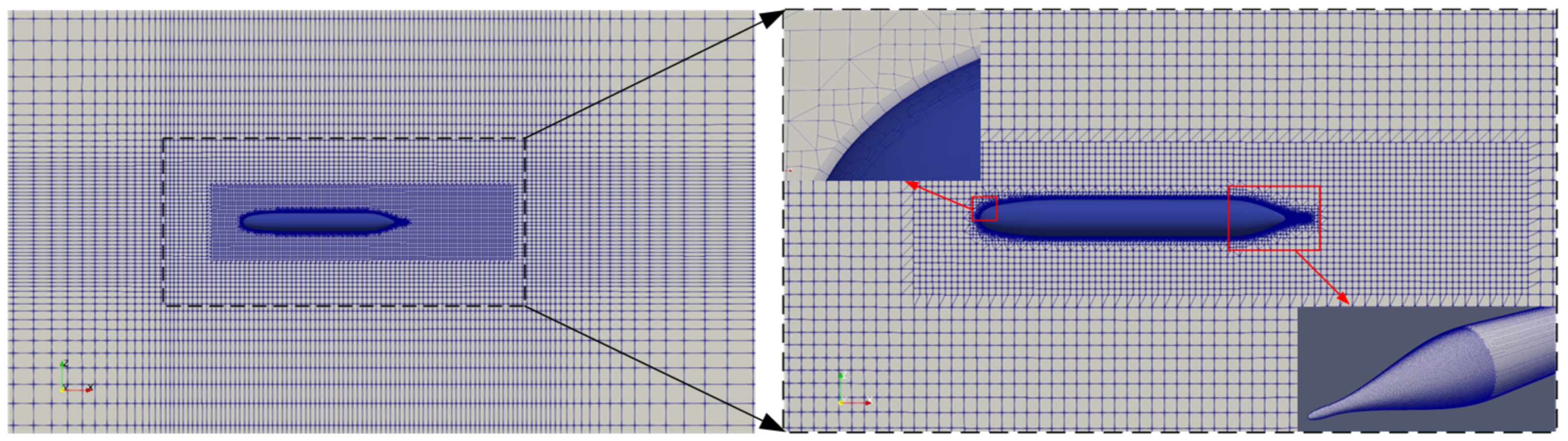
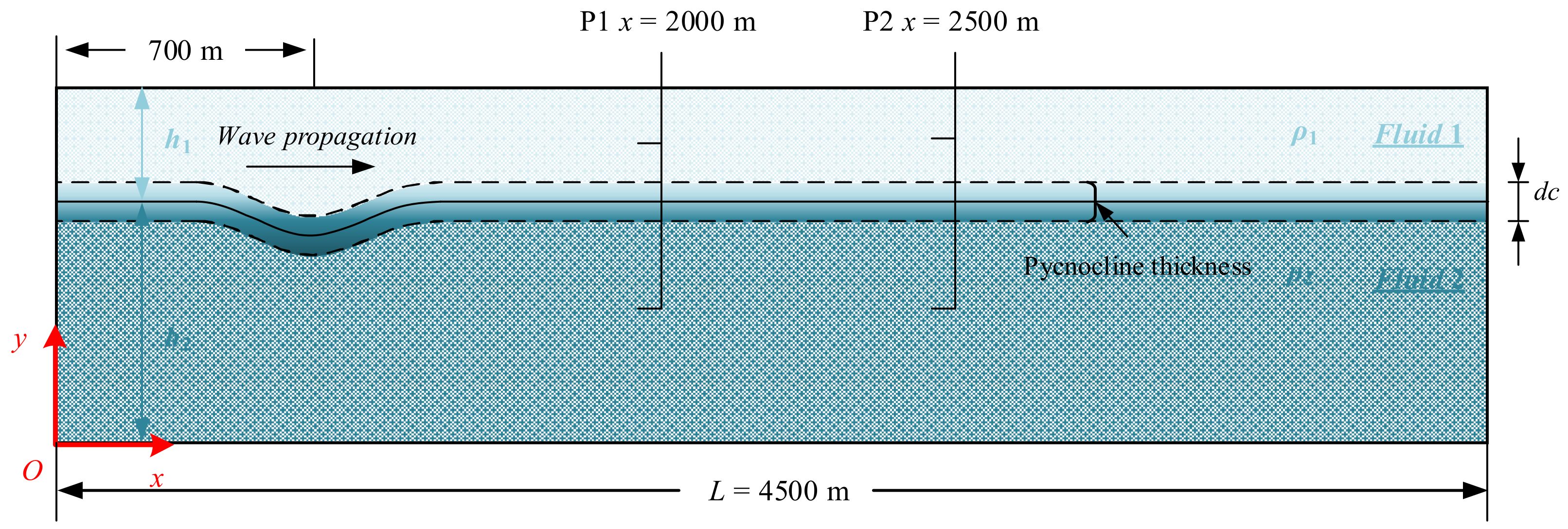
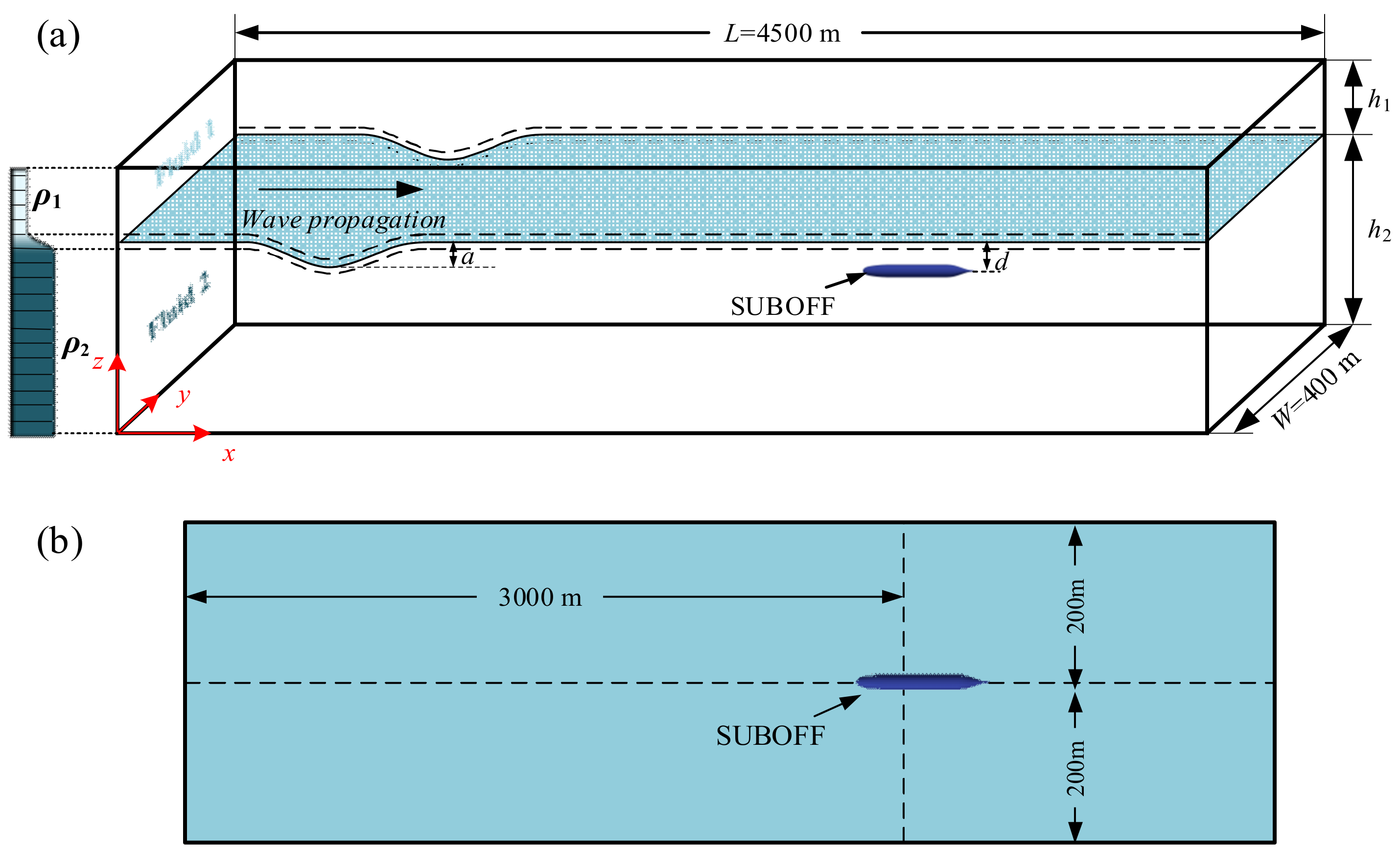
3.1. Computational Domain and Grids

The vehicle model used in the present research is the standard submarine model proposed by the Defense Advanced Research Project Agency (DARPA). The geometry of the DARPA SUBOFF was defined by polynomial equations. In this study, only the geometry of the bare hull (AFF-1) was tested. The length of the model is L_pp = 4.356 m, and the maximum diameter of the model is D = 0.508 m. More details can be found in Groves et al. [25]. The computational domain size was defined following ITTC guidelines [26]. As shown in Figure 1, the half-domain was used to save the CPU time, where the width of the computational domain is 2L_pp. The inlet boundary is 3L_pp away from the hull, while the outlet boundary is 4L_pp away from the hull to make sure the boundaries are placed far enough from the submarine. As seen in Figure 2, the grids were generated by snappyHexMesh. The grid size was controlled by background grid size and refinement levels. Here, four refinement levels were applied on the head of the submarine, and five refinement levels were applied on the tail of the submarine to capture the surface of the submarine with large curvature changes.

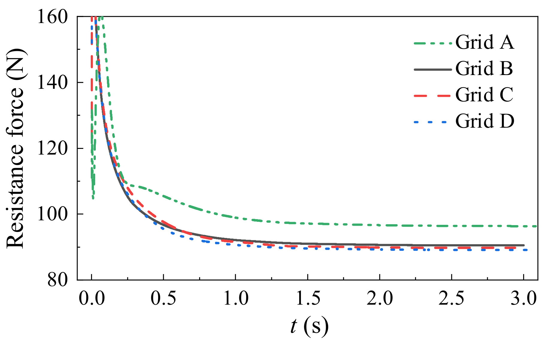
3.2. Grid Convergence Study

The SUBOFF-AFF-1 submarine model in single-layer flow was employed to simulate the resistance at a navigation speed of 6 knots. Four background grid sizes were applied to carry out the convergency study. The background sizes are 90 mm for Grid A, 70 mm for Grid B, 65 mm for Grid C, and 60 mm for Grid D, with the maximum courant number of 0.8. The relative error was defined as the difference between the numerical results and the experimental data.

The total resistance forces of the submarine navigating at different grid sizes are given in

Table 1. Grid convergence study.

Label	Grid Size (mm)	Grid Number (×104)	Resistance (N)	Experiment (N)	Relative Error (%)
Grid A	90	57.8	96.42	87.4	10.32
Grid B	70	109.8	90.52	87.4	3.57
Grid C	65	169.1	89.76	87.4	2.7
Grid D	60	271.5	89.11	87.4	1.95

. Figure 3 shows the time series of the resistance force on the submarine using different sizes of grids. From the relative error and the resistance forces for Grid C and D, respectively in Table 1 and Figure 3, it can be found that the numerical results achieved convergence with the decrease in grid sizes. Considering the calculation accuracy and efficiency, Grid C was adopted in the following research.

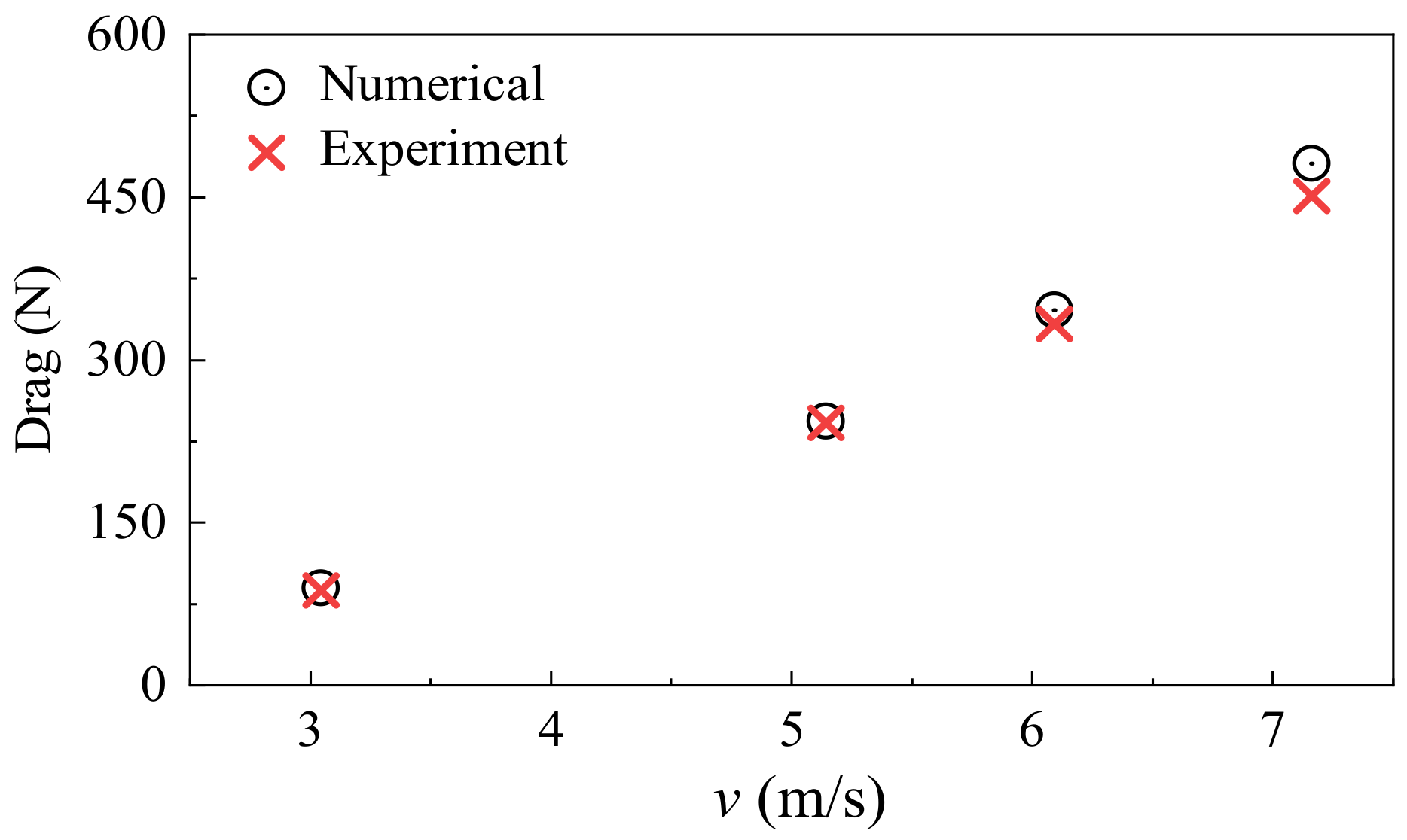
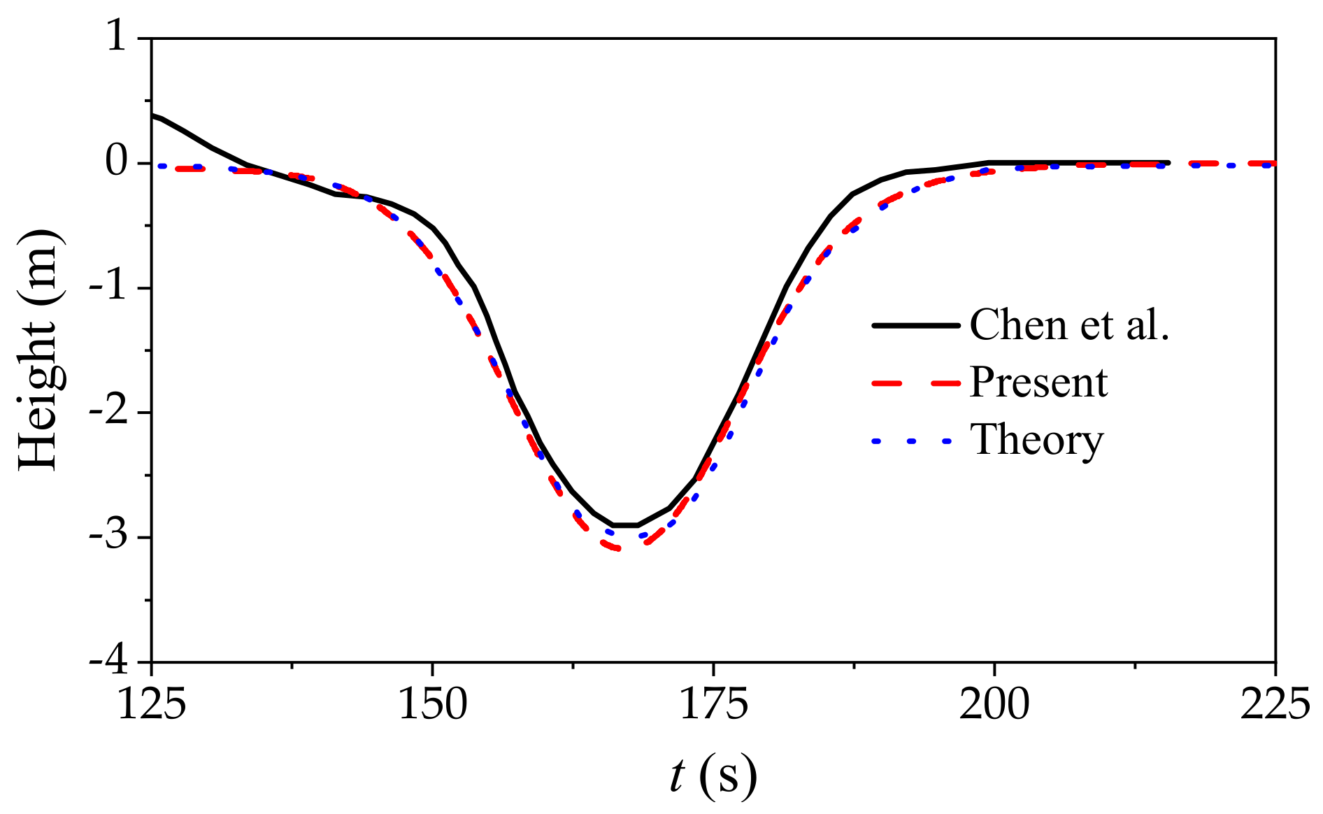
3.3. Comparison between Numerical and Experimental Results

To further verify the accuracy of this newly developed numerical model, the calculated resistance of the SUBOFF was compared with the experimental results in Liu et al. [27]. The speeds of the submarine are v = 3.046 m/s, 5.144 m/s, 6.091 m/s and 7.161 m/s, respectively. Figure 4 shows the numerical results and measured resistance on the submarine. The relative errors between the numerical results and the experimental results are shown in

Table 2. Relative errors between the numerical results and the experimental results.

Velocity (m/s)	Numerical Results (N)	Experimental Results (N)	Relative Error (%)
3.046	89.76	87.4	2.7
5.144	243.59	242.2	0.6
6.091	345.975	332.9	3.9
7.161	481.226	451.5	6.5

. From Figure 4 and Table 2, it can be found that the numerical results agree well with the experimental results, which validates the accuracy of the proposed numerical model.

4. Results and Discussion

Based on the proposed numerical model, the interaction between the ISWs and the moving submarine was investigated. Here, the forward speed of the submarine is equivalent to a current. First, a series of ISWs were generated using the established wave tank. Then, the interaction between the moving submarine and the ISWs against different pycnocline thicknesses and different moving speeds was investigated.

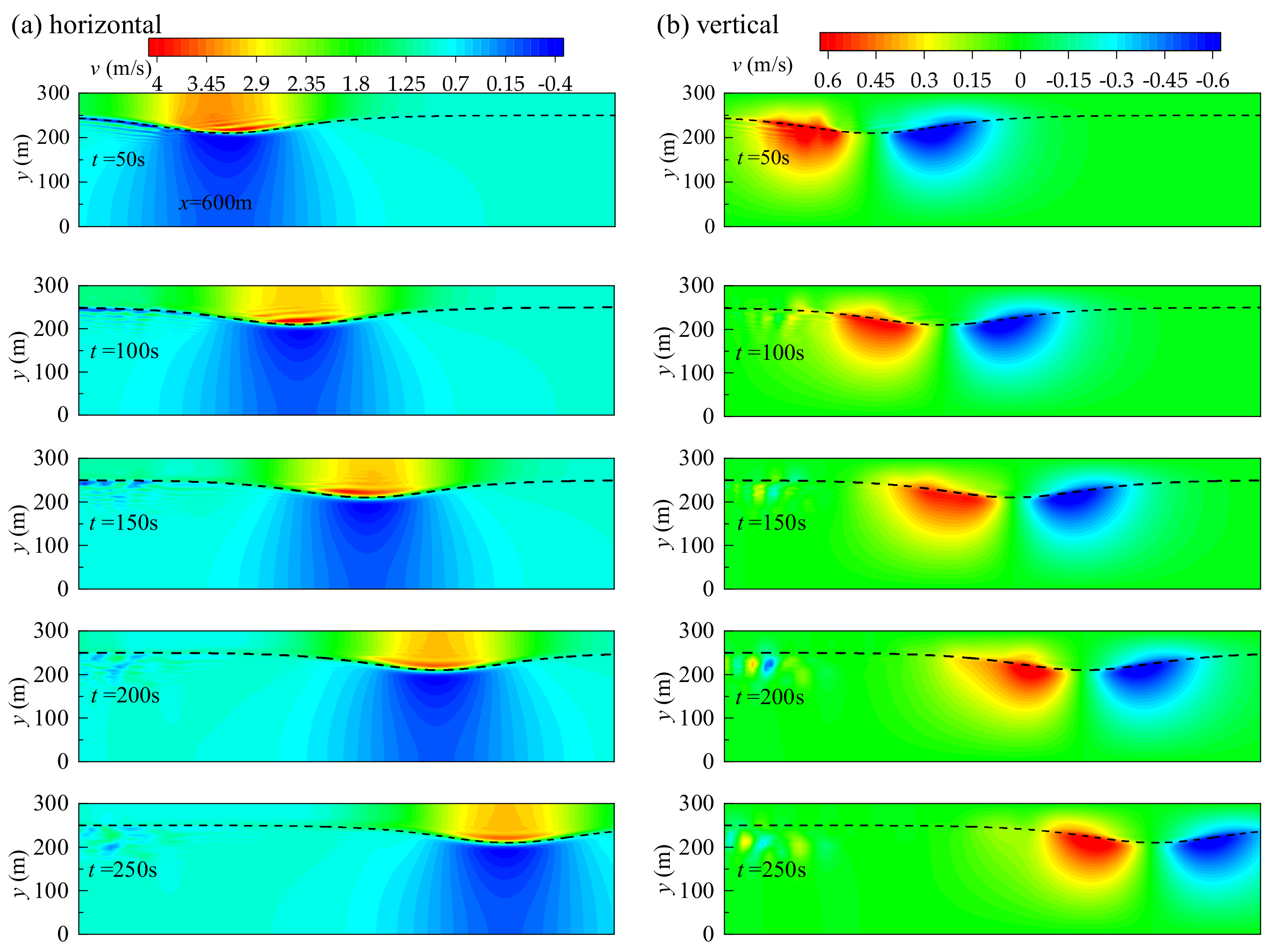
4.1. ISW Propagation under the Action of Current

As Figure 5 shows, a 2D numerical ISW wave tank was established. The length of the wave tank is L = 4500 m. The depth of the upper layer and the lower layer are h₁ = 50 m and h₂ = 250 m, respectively. The densities of the upper layer and lower layer are ρ₁ = 996 kg/m³, ρ₂ = 1030 kg/m³, respectively. The wave amplitude is a = 40 m, and the initial position of the ISW is x = 700 m. The ISWs propagate from left to right. Two probes were located on x = 2000 m, and x = 2500 m. The grid was uniform in x-direction and y-direction, and the grid sizes are Δx = 20 m, and Δy = 2.5 m. Slip boundaries were applied to the bottom and the top boundaries. Cyclic boundaries were applied to the inlet and outlet boundaries.

Two kinds of current velocities v = 0 m/s and v = 0.5 m/s are considered, which were named A1 and A2 as shown in

Table 3. Velocity of current and pycnocline thickness in each simulation.

Label	Velocity (m/s)	Pycnocline Thickness (m)
A1	0	5
A2	0.5	5
A3	1	5
A4	1	10
A5	1	15

. The pycnocline thickness was set as d_c = 5 m. Figure 6 shows the time series of wave height for conditions A1 and A2 at different probes, respectively. The results indicate that the waveform of the internal solitary wave remains stable during the propagation process, and the decay rate is less than 1%. Taking A1 as an example, the decay rate of wave amplitude between P1 and P2 is 0.5%. The comparison between Case A1 and Case A2 shows that the influence of current on waveform can be neglected. The numerical results agree well with the theoretical results, which validate the ISW generation method proposed in this study.

Figure 7 shows the horizontal and vertical velocity fields of Case A3 shown in Table 3 at different times. At t = 50 s, the horizontal velocity field is not continuous in the interface areas between the upper layer and the lower layer. With the propagation of the ISW, the interface becomes smooth after t = 250 s, then the waveform of ISW becomes stable. It should be noted that the black dashed line in each subfigure represents the theoretical wave profile, which agrees well with the numerical interface between the upper layer and the lower layer.

Figure 8 shows the density distribution during the propagation of ISWs for Cases A4 and A5 shown in Table 3, respectively. It should be noted that different pycnocline thicknesses d_c = 10 m and 15 m were used for Cases A4 and A5. The density contour indicates that the waveform remains stable without breaking during the propagation of ISWs. It can also be found that the thickness of the pycnocline increases at the rear of ISWs due to miscibility. The theoretical wave profiles were given as black dashed lines in each subfigure, which agree well with the numerical results.

To further validate the ISW generation method proposed in this study, the calculated wave profile was compared with Chen’s results [11]. The densities of upper layer and lower layer are ρ₁ = 1021 kg/m³ and ρ₂ = 1027 kg/m³, respectively. The depths of the upper layer and the lower layer are h₁ = 1.75 m and h₂ = 10.5 m, respectively. The wave height is a = 3 m with the current velocity v = 0.641 m/s. Figure 9 shows the wave profile obtained from the present method, Chen’s method [11], and the theoretical solution. The numerical results in this paper agree better with the theoretical results than Chen’s results. Therefore, the generation method of the ISWs coupled with the current developed in this paper is stable and accurate.

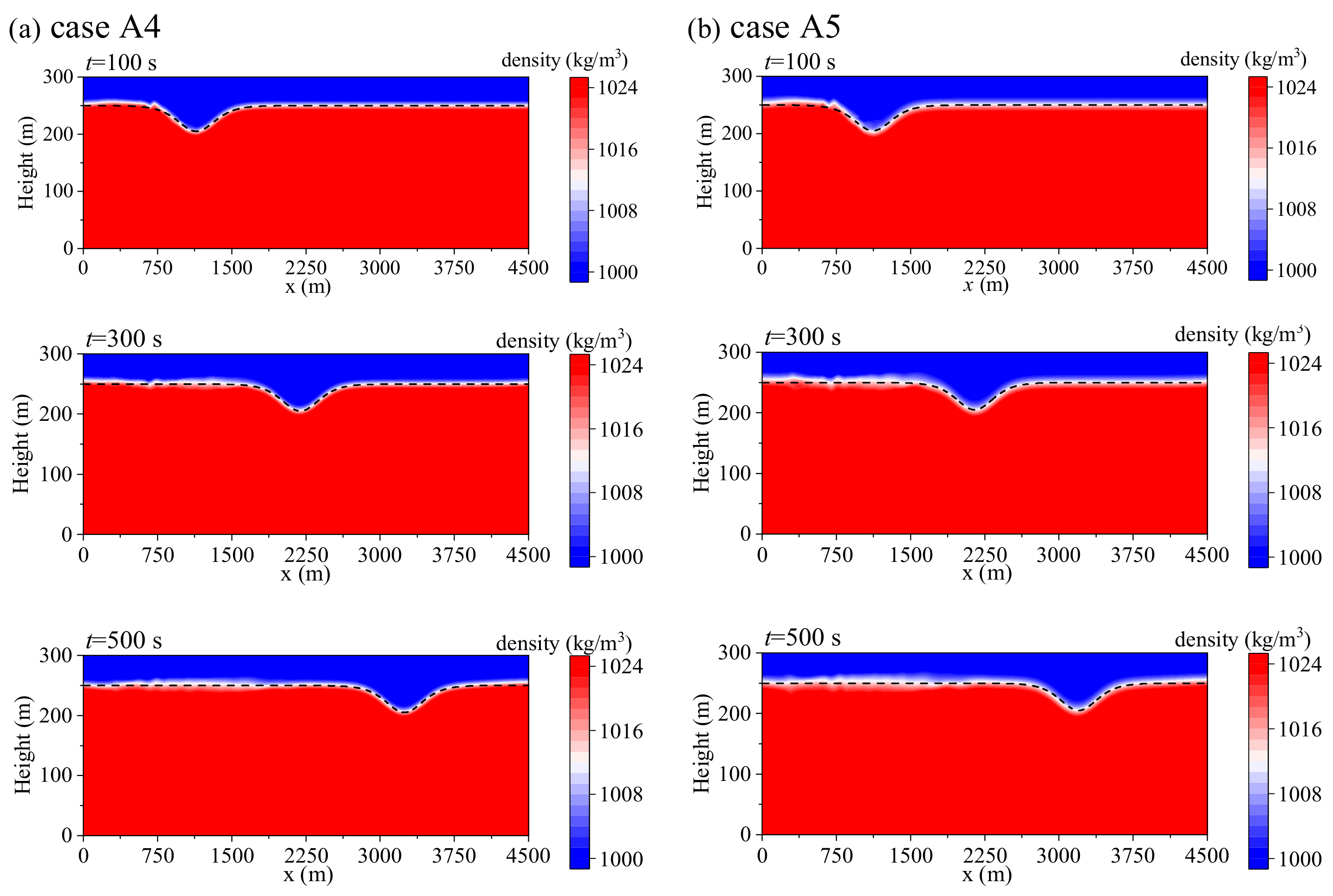
4.2. Interaction between Submarine and ISWs with Different Pycnocline Thickness

As shown in Figure 10 and Figure 11, a 3D ISW numerical wave tank was established. The length of the tank is L = 4500 m, the width of the tank is W = 400 m, and the depths of the upper layer (h₁) and lower layer (h₂) are 50 m and 250 m, respectively. The densities of the upper layer (ρ₁) and lower layer (ρ₂) are 996 kg/m³ and 1025 kg/m³, respectively. The length of SUBOFF model is L_pp = 87.12 m, and the maximum diameter is D = 10.16 m. The location of the submarine is 3000 m away from the inlet boundary. The center of rotation is a distance of L_pp/3 from the bow, and the submergence of the submarine is d = 20 m. The cyclic boundary was applied to the inlet and outlet boundaries, while the slip boundary was applied to other boundaries.

The loads on the submarine during the propagation of ISWs mainly consist of three components: horizontal forces F_x, vertical forces F_z and torque M_y. The nondimensional form of these forces can be written as follows [7]:

$$C_x=\frac{F_x}{{\rho }_{2}gV},$$

(22)

$$C_z=\frac{F_z}{{\rho }_{2}gV},$$

(23)

$$C_m=\frac{M_y}{{\rho }_{2}gVL},$$

(24)

where V is the displacement of the submarine.

The interaction between the submarine and the ISWs against different pycnocline thicknesses as shown in

Table 4. Three cases of the submarine against ISWs with different pycnocline thickness.

Label	Velocity (m/s)	Pycnocline Thickness (m)
B1	0	5
B2	0	10
B3	0	15

was studied. It should be noted that the current speed was set as 0. First, the horizontal forces C_x on the submarine induced by ISW were investigated, as shown in Figure 11. The propagation of the ISWs can be divided into five stages. The five stages for Case B1 were marked as I, II, III, IV, and V as an example. The adjacent stages were separated by vertical dotted lines, where the corresponding time was marked out. The demarcation point of the two adjacent stages was labelled with ①, ③, ⑤ and ⑦. It can be seen from the results of Case B1 that in the first stage I (0 s < t < 498 s), the submarine and the internal solitary wave approach each other. In the second stage II (498 s < t < 529 s), the submarine passes through the interface of the ISW for the first time. In the third stage III (529s < t < 588s), the submarine navigates in the upper layer. In the fourth stage IV (588 s< t <644 s), the submarine navigates from the upper layer to the lower layer. In the fifth stage Ⅴ (t > 644 s), the submarine gradually navigates away from the ISW.

Figure 12 shows the dynamic pressure induced by ISW at key times ①–⑦. In Figure 11, the C_x increases in stage I and reaches the negative maximum at ① when the submarine encounters the interface of ISW, as shown in Figure 12a. It is noted that the dynamic pressure on the head of the submarine is much smaller than that on the tail, which leads to negative C_x. In stage II, the submarine gradually enters the upper layer. The dynamic pressure on the head gradually becomes larger than that on the tail, thus the C_x gradually reverses to positive and reaches the positive maximum at ③ when the submarine enters the upper layer totally, as seen in Figure 12c. In stage III, the dynamic pressure on the head gradually becomes smaller than that on the tail, thus the positive C_x decreases and reaches the negative maximum at ⑤ when the submarine encounters the pycnocline, as seen in Figure 12e. In stage IV, the submarine passes through the interface of the ISW again. The dynamic pressure on the head becomes larger than that on the tail, thus the C_x increases and reaches the positive maximum at ⑦ when the submarine enters the lower layer, as seen in Figure 12g. In stage V, the dynamic pressure both on the head and the tail tends to be 0, thus the C_x gradually becomes 0. Besides, three zero-crossing points are labeled as ②, ④, and ⑥ in Figure 11. Looking at the dynamic pressure of ②, ④, and ⑥ in Figure 12b,d,f, respectively, it can be found that the submarine is located at the pycnocline for ② and ⑥, while the submarine is at the pressure center for ④. The dynamic pressure on the head and the tail of the submarine are balanced at ②, ④, and ⑥, which leads to zero C_x. Comparing the C_x of Case B2 and Case B3 to that of Case B1 in Figure 11, it can be found that the extreme values of |C_x| decrease with the increment of pycnocline thickness. Besides, the occurrence of extreme values of C_x is delayed by the increment of pycnocline thickness.

Then, the vertical forces C_z on the submarine induced by ISW were investigated, as shown in Figure 13. Similar to the C_x, the change of the C_z can also be generally divided into five stages, which were marked as I, II, III, IV, and V for Case B1 as an example. In stage I, the submarine navigates in the lower layer. The dynamic pressures on the top and the bottom of the submarine are both negative, thus the C_z is small until the submarine encounters the interface of the ISW at ① referring to Figure 12a. In stage II, the |C_z| sharply increases due to the increment of the dynamic pressure on the top of the submarine. In stage III, the submarine navigates in the upper layer, and the difference in the dynamic pressure between the top and the bottom of the submarine changes little. Thus, the C_z is stable in this period. In stages IV and V, the changes of C_z are contrary to those in stages II and I, respectively. It is noted that the direction of the vertical force C_z is downward in the five stages, which can cause the sinking of the submarine. The values of C_z are one order of magnitude higher than that of C_x. From looking at the C_z of Cases B2 and B3 in Figure 13, it can be found that, with the increment of the pycnocline thickness, the maximum values of |C_z| decrease. The occurrence of extreme values of C_z is also delayed by the increment of pycnocline thickness, which is similar to that of C_x.

Figure 14 is the time series of the torque C_m on the submarine against different pycnocline thicknesses. As seen in the results of Case B1, similar to the tendency of the vertical force C_z, the C_m changes significantly when the submarine encounters the ISW after ①. The C_m increases anticlockwise when the submarine passes through the interface in stage II, and the C_m increases clockwise when the submarine travels from the upper layer into the lower layer in stage IV. In stage III, the C_m becomes stable, which is similar to that of C_z. Some schematic diagrams of the torque on the submarine for six typical times in stages II and IV are shown in Figure 14 to demonstrate the change laws of C_m. As seen in the results of Case B2 and B3, it can also be found the decrease of maximum values of C_m and the delay of the extreme values of C_m with the increment of pycnocline thickness.

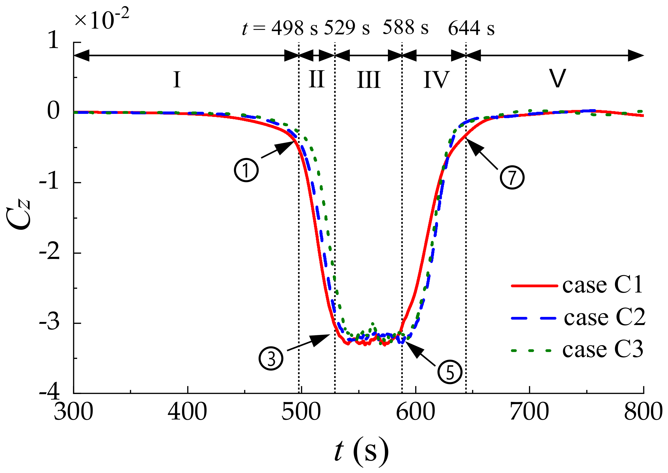
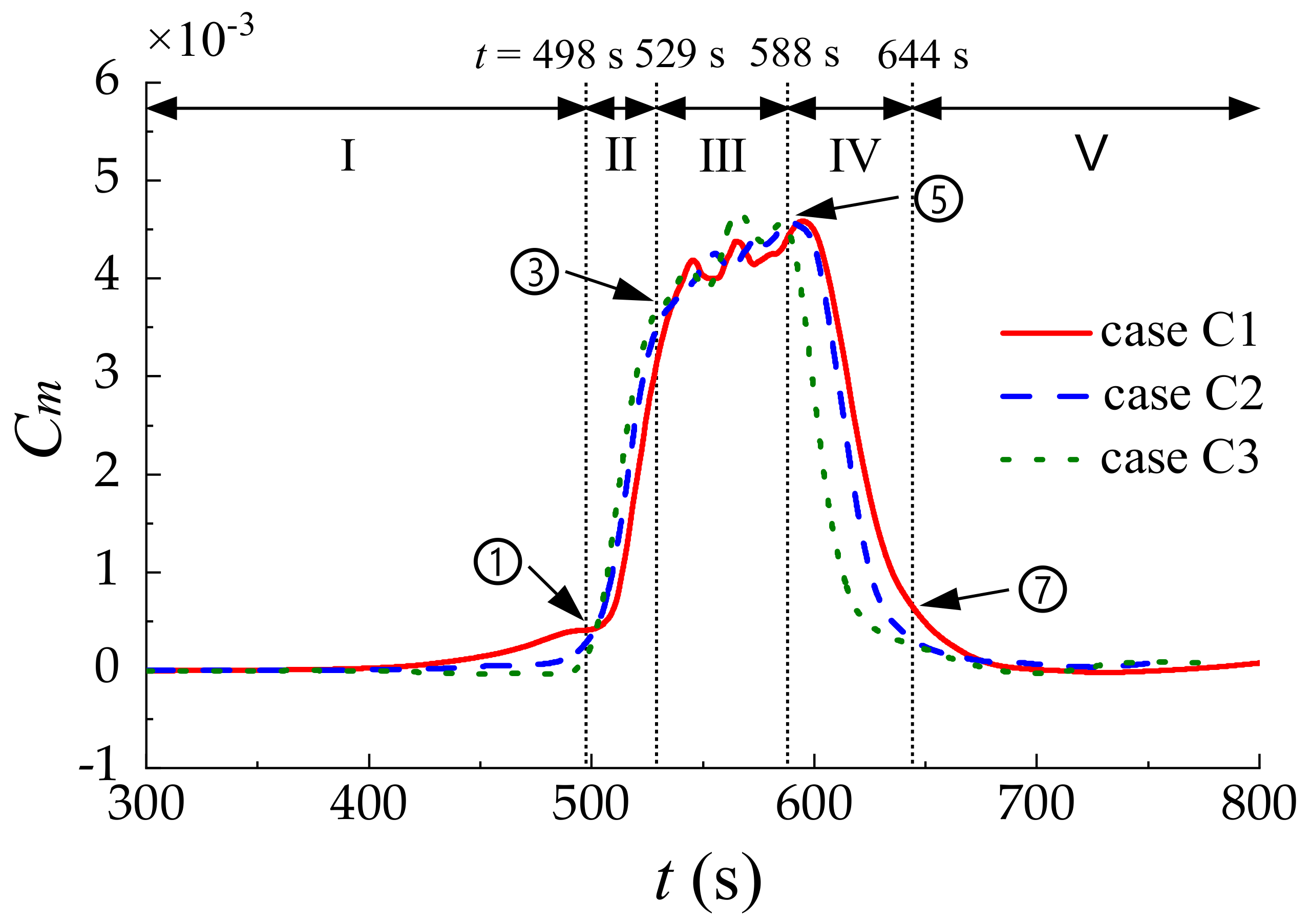
4.3. Interaction between ISWs and the Submarine with Different Velocities

The interaction between the submarine and the ISWs against different velocities as shown in

Table 5. Three cases of the submarine against ISWs with different velocity.

Label	Velocity (m/s)	Pycnocline Thickness (m)
C1	0	5.0
C2	0.5	5.0
C3	1	5.0

was studied. It is noted that Case C1 in Table 5 is the same as Case B1 in Table 4. First, the horizontal force C_x on the submarine induced by ISW was investigated, as shown in Figure 15. The propagation of the ISWs was also divided into five stages. The five stages for Case C1 were marked as I, II, III, IV, and V as an example, which is the same as that in Figure 11 for Case B1. In Figure 15, it can be found that the results of Case C2 and C3 move upward compared to that of Case C1 due to the navigating resistance. With the increments of navigation speed, the |C_x| decreases for ① but increases for ③, ⑦. The |C_x| at ① for Case C1 is −1.4 × 10⁻³. Compared with Case C1, the |C_x| at ① for Case C3 is reduced by 59.28%. Besides, the |C_x| at ③ for Case C3 increases 53.8% over that of Case C1. It is noted that the C_x for ⑤ can change from negative to positive with the increment of navigation speed.

The difference between Case C1 and C3 is that the flow speed in Case C3 is 1.0 m/s but there is no flow in Case C1. However, as can be seen in Figure 15, the C_x of Case C3 cannot be simply regarded as the linear superposition of Case C1 and the steady flow resistance. To further validate this conclusion, the C_x of Case C1 and Case C3 were compared in Figure 16. The steady flow resistance on the submarine is C_x = 7.8 × 10⁻⁵ when the velocity of current is 1 m/s (Case C3). The linear superposition of the C_x of Case C1 (ISWs only) and the C_x induced by current only (1 m/s) is drawn as the black dotted line in Figure 16. The time series of Cx for Case C3 can be divided into two parts by t = 425 s. At t < 425 s, the submarine is far from the ISW, and the C_x is only induced by the current. Thus, the C_x for Case C3 (green dashed line) agrees with the linear superposition of the C_x of Case C1 (ISWs only) and the C_x induced by current only (black dotted line). At t > 425 s, the ISW gradually affects the submarine. However, the green dashed line does not agree with the black dotted line, which means the coupling of ISWs and the current is nonlinear.

Figure 17 and Figure 18 show the comparison of the vertical force C_z and pitching moment C_m on the submarine with different speeds. The results show that the tendency of all three cases is similar. Besides, the extreme values of C_z and C_m at ③ and ⑤ are similar, which means the current has little influence on C_z and C_m.

5. Conclusions

An ISWs-current coupled numerical model was proposed to simulate the hydrodynamic interaction problems between a moving submarine and ISWs. In the present model, the initial velocity field was derived by the superposition of the velocity field obtained from the eKdV theory and the velocity field of the current. The present numerical model was validated by convergence analysis and the experimental results. Based on the established numerical model, the interaction between the moving submarine and the ISWs against different pycnocline thicknesses and different moving speeds was investigated. The interaction process between the submarine and the ISWs can be divided into five stages. In each stage, the horizontal force C_x, the vertical force C_z and the torque C_m on the submarine combined with the dynamic pressure distribution of the fluid field were analyzed. The main conclusions of this study can be summarized as follows:

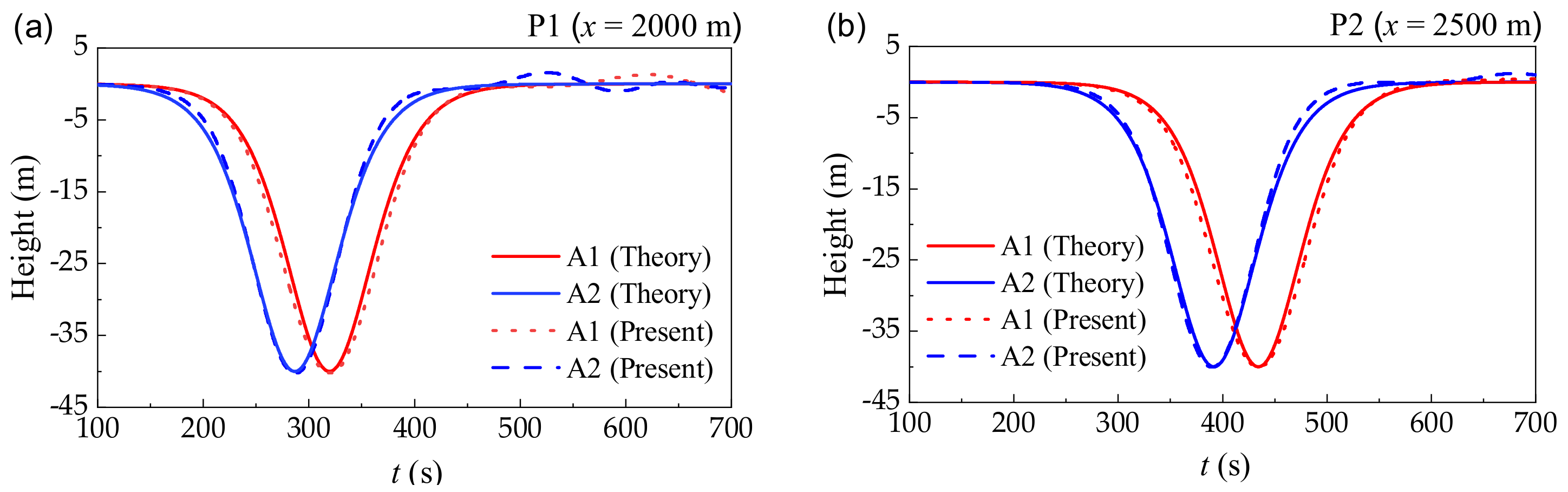
• A series of ISWs coupled with the current against various flow speeds and pycnocline thicknesses were made using the proposed numerical method. Based on the waveform analysis of the ISWs and the comparison with theoretical results, the propagation of the ISWs was validated to be accurate and stable.
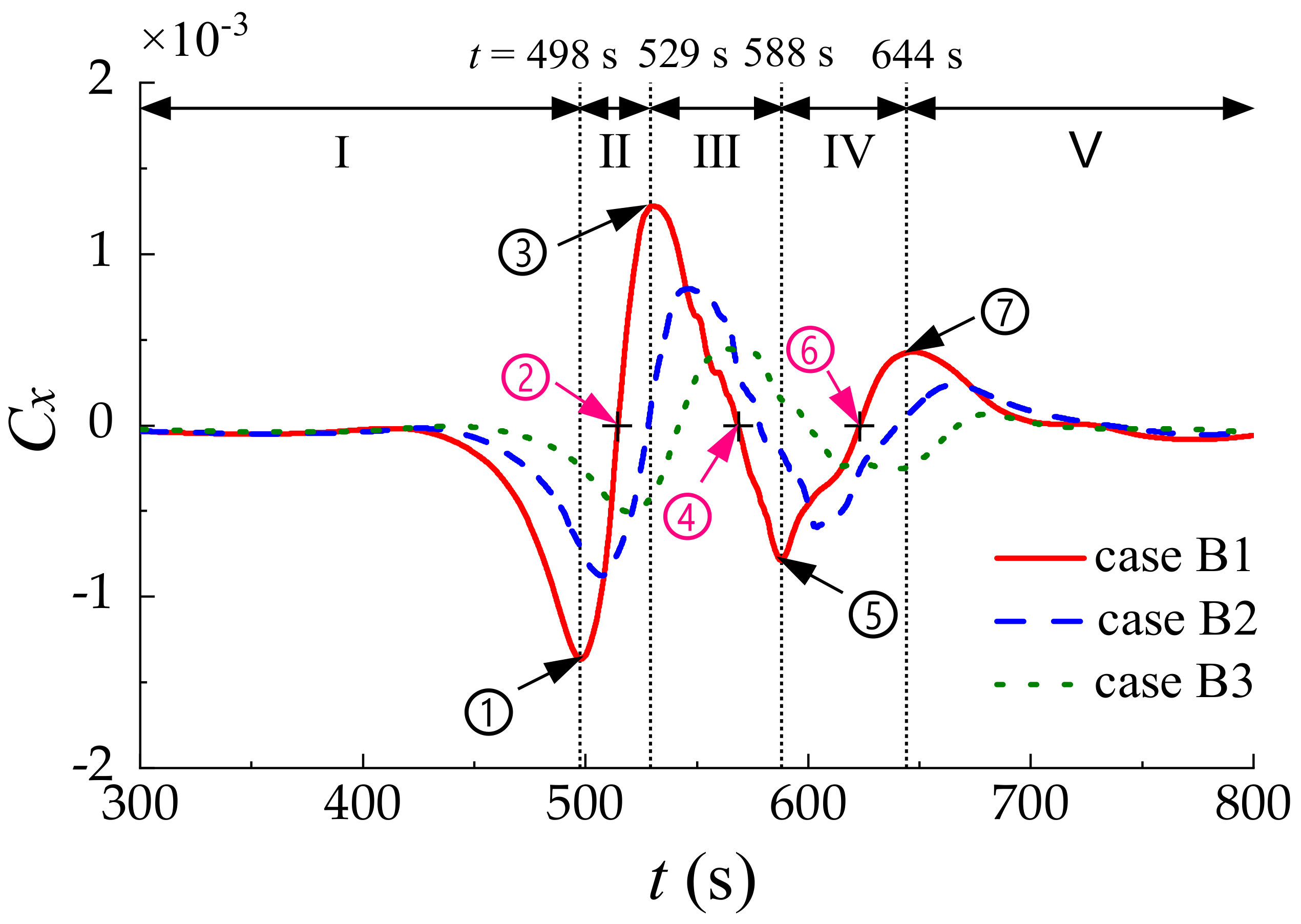
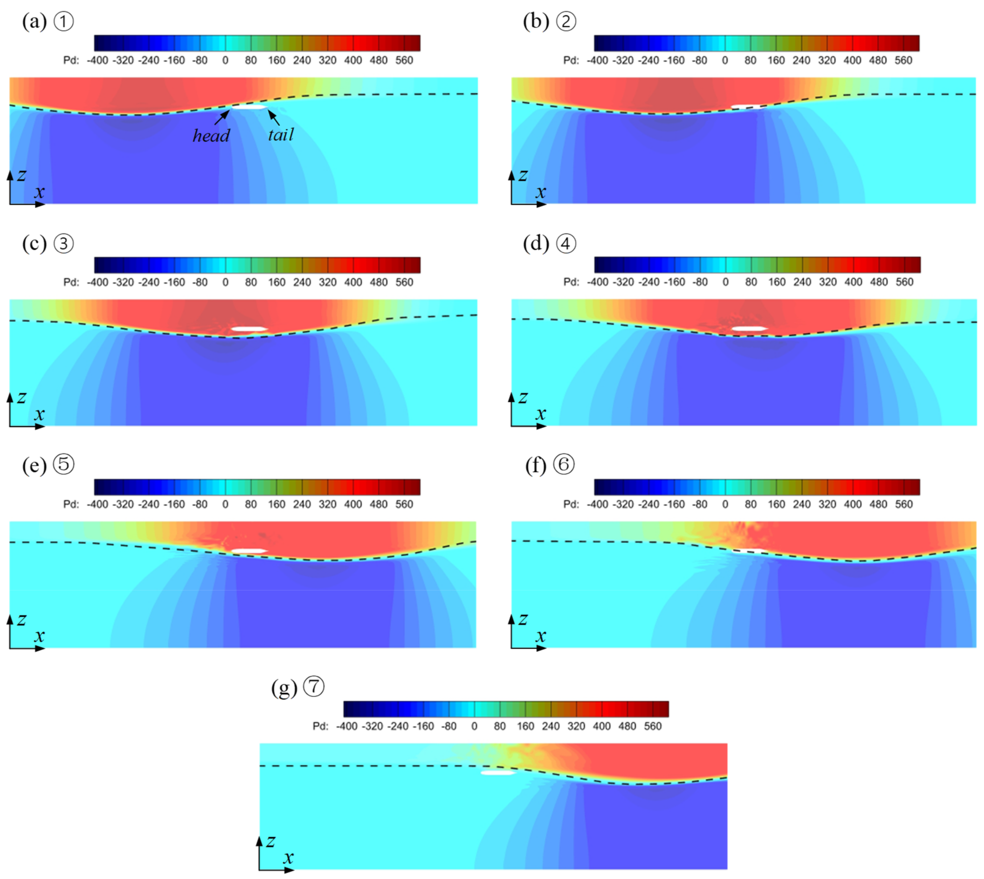
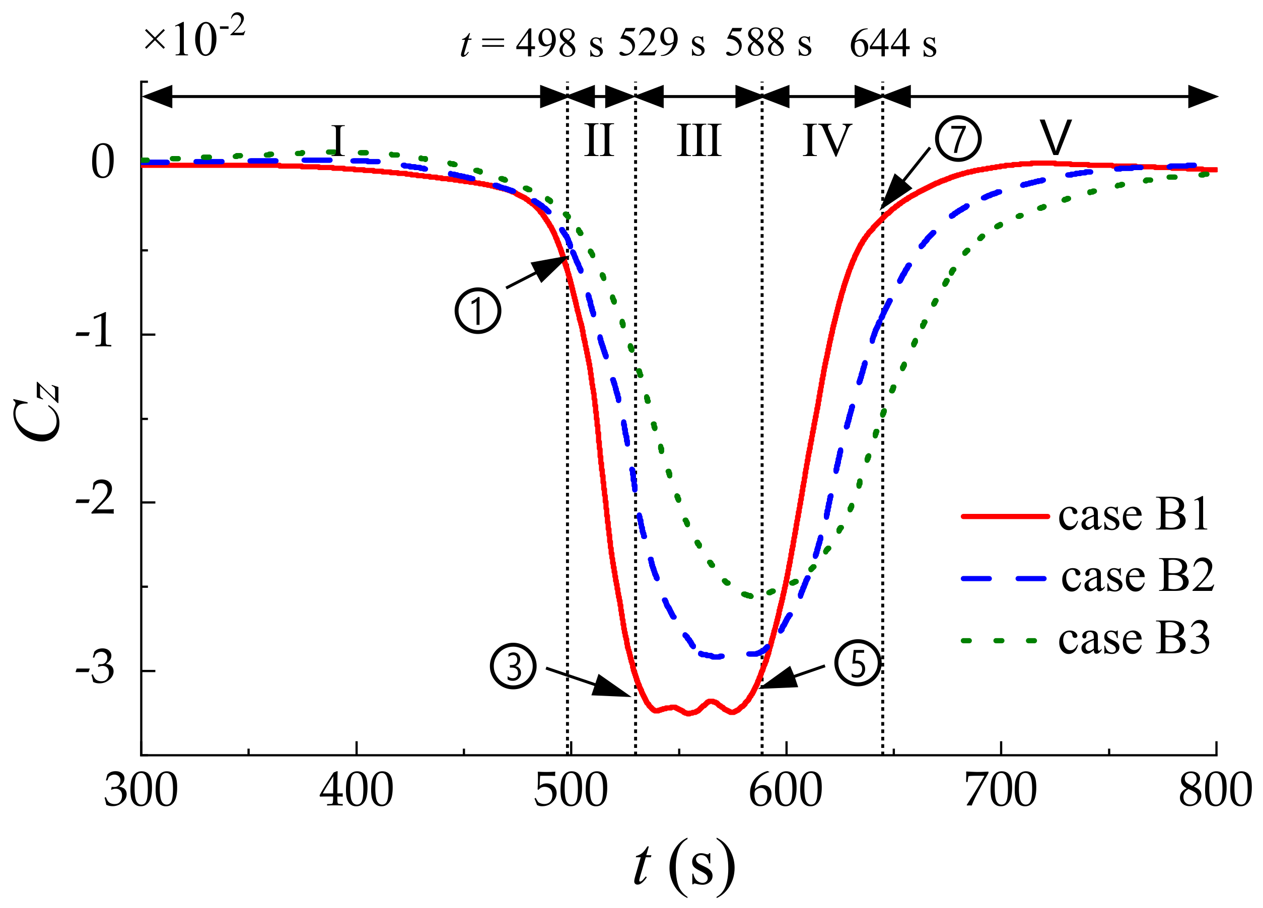
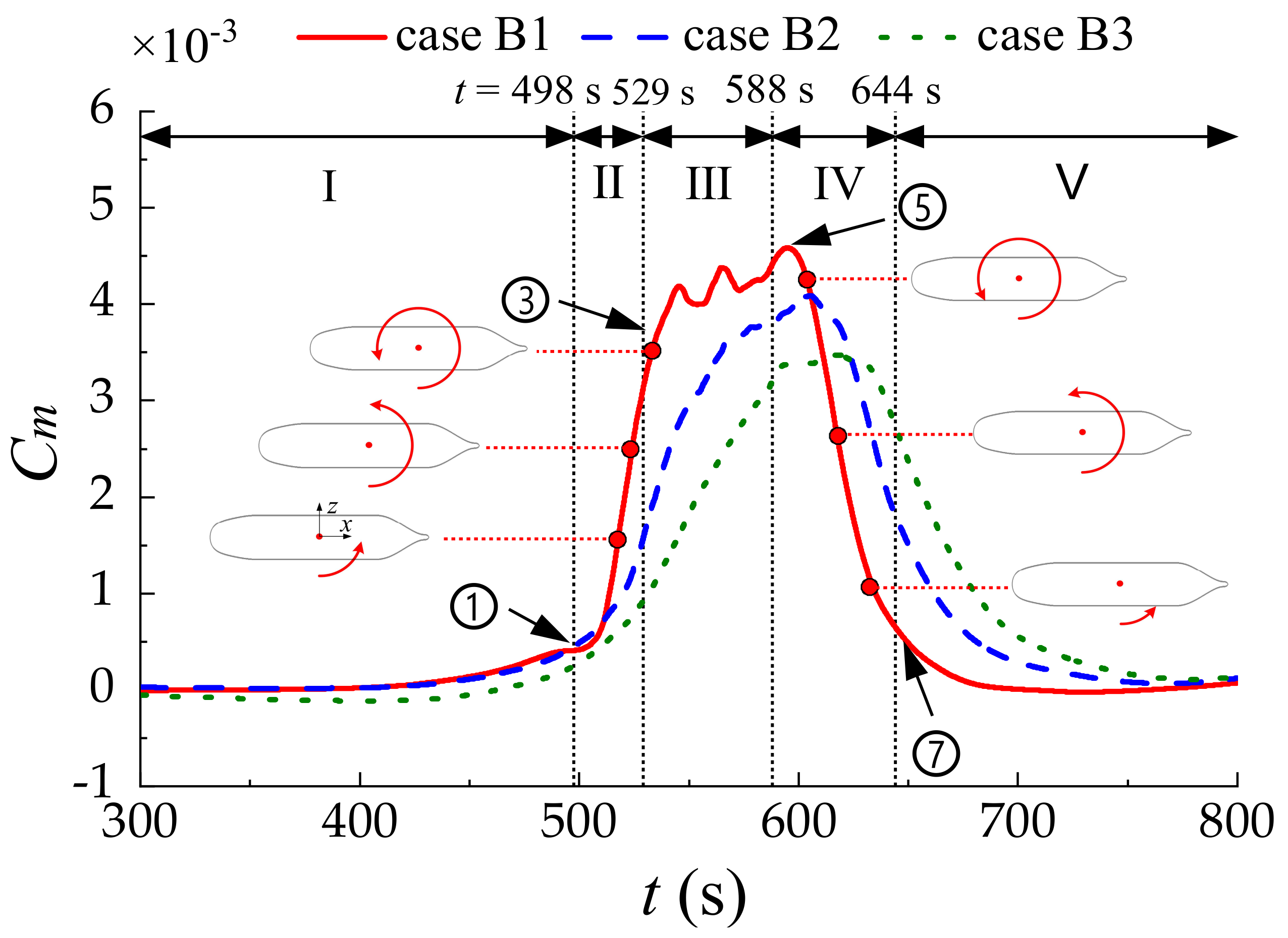
• The ISWs-induced horizontal force C_x, the vertical force C_z and the torque C_m on the submarine against various pycnocline thicknesses were investigated. It was found that the hydrodynamic forces are closely related to the dynamic pressure around the submarine. The direction of the vertical force C_z is downward in the five stages, which can cause the sinking of the submarine. Besides, the maximum values of |C_x|, |C_z|, |C_m| decrease with the increment of the pycnocline thickness.
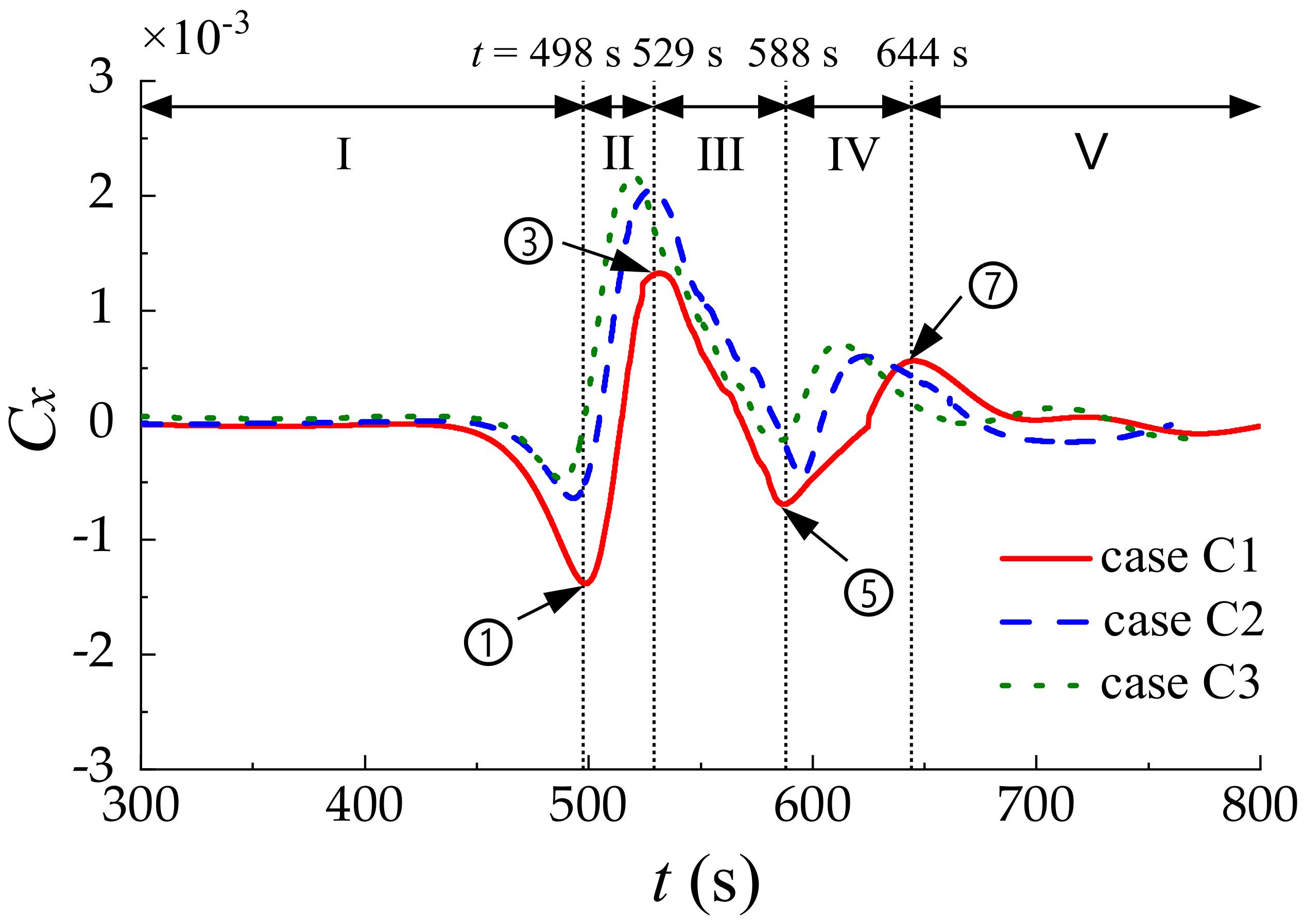
• The horizontal force C_x, the vertical force C_z and the torque C_m on the submarine induced by the coupling of the ISWs and the current were studied. Different flow speeds were considered to demonstrate their effects on the hydrodynamic forces. It was found that peak values of C_x increase with the increment of the flow speed. Moreover, the flow speed performs significant effects on C_x but ignorable effects on C_z and C_m.
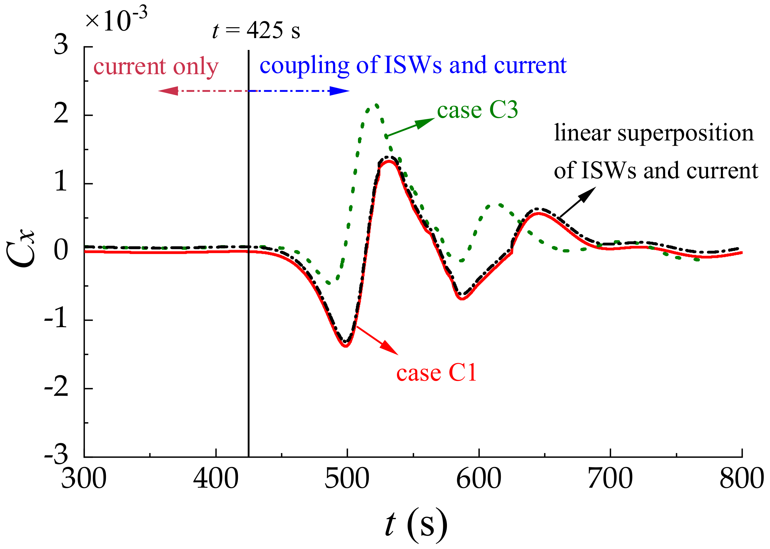
• The interaction between the submarine and the ISWs coupled with the current is complicated. When the submarine is far from the ISWs, the hydrodynamic forces on the submarine can be thought to be caused only by the current. However, when the submarine encounters the ISWs, the hydrodynamic forces on the submarine cannot be simply regarded as the superposition of the ISWs-induced forces and the steady flow resistance, which means the coupling of ISWs and the current is nonlinear.

References

1. Dong, J.; Zhao, W.; Chen, H.; Meng, Z.; Shi, X.; Tian, J. Asymmetry of internal waves and its effects on the ecological environment observed in the northern South China Sea. Deep. Sea Res. Part I Oceanogr. Res. Pap. 2015, 98, 94–101. [Google Scholar] [CrossRef]
2. Zhang, H.; Li, J. Wave loading on floating platforms by internal solitary waves. In Proceedings of the Fifth International Conference on Fluid Mechanics, Shanghai, China, 15–19 August 2007; pp. 304–307. [Google Scholar]
3. Song, Z.J.; Teng, B.; Gou, Y.; Lu, L.; Shi, Z.M.; Xiao, Y.; Qu, Y. Comparisons of internal solitary wave and surface wave actions on marine structures and their responses. Appl. Ocean. Res. 2011, 33, 120–129. [Google Scholar] [CrossRef]
4. Wang, X.; Zhou, J.F.; Wang, Z.; You, Y.X. A numerical and experimental study of internal solitary wave loads on semi-submersible platforms. Ocean. Eng. 2018, 150, 298–308. [Google Scholar] [CrossRef]
5. Wang, X.; Zhou, J.F. Numerical and experimental study of internal solitary wave loads on tension leg platforms. J. Hydrodyn. 2021, 33, 93–103. [Google Scholar] [CrossRef]
6. Chen, M.; Chen, K.; You, Y.X. Experimental investigation of internal solitary wave forces on a semi-submersible. Ocean. Eng. 2017, 141, 205–214. [Google Scholar] [CrossRef]
7. Ding, W.; Ai, C.F.; Jin, S.; Lin, J.B. 3D numerical investigation of forces and flow field around the semi-submersible platform in an internal solitary wave. Water 2020, 12, 208. [Google Scholar] [CrossRef] [Green Version]
8. Wang, T.; Huang, X.; Zhao, W.; Zheng, S.H.; Yang, Y.C.; Tian, J.W. Internal Solitary Wave Activities near the Indonesian Submarine Wreck Site Inferred from Satellite Images. J. Mar. Sci. Eng. 2022, 10, 197. [Google Scholar] [CrossRef]
9. Gong, Y.K.; Xie, J.S.; Xu, J.X.; Chen, Z.W.; He, Y.H.; Cai, S.Q. Oceanic internal solitary waves at the Indonesian submarine wreckage site. Acta Oceanol. Sin. 2022, 41, 109–113. [Google Scholar] [CrossRef]
10. Fu, D.M.; You, Y.X.; Li, W. Numerical simulation of internal solitary waves with a submerged body in a two-layer fluid. Ocean. Eng. 2009, 37, 38–44. [Google Scholar]
11. Chen, J.; You, Y.X.; Liu, X.D.; Wu, C.S. Numerical simulation of interaction of internal solitary waves with a moving submarine. Chin. J. Hydrodyn. 2010, 25, 344–350. [Google Scholar]
12. Huang, M.M.; Zhang, N.N.; Zhu, A.J. Numerical simulation of the interaction motion features for a submarine with internal solitary wave. In Proceedings of the 30th International Ocean and Polar Engineering Conference, OnePetro, Shanghai, China, 11–16 October 2020; pp. 1805–1812. [Google Scholar]
13. Li, J.Y.; Zhang, Q.H.; Chen, T.Q. Numerical Investigation of Internal Solitary Wave Forces on Submarines in Continuously Stratified Fluids. J. Mar. Sci. Eng. 2021, 9, 1374. [Google Scholar] [CrossRef]
14. Li, J.Y.; Zhang, Q.H.; Chen, T. ISWFoam: A numerical model for internal solitary wave simulation in continuously stratified fluids. Geosci. Model Dev. Discuss. 2021, 15, 105–127. [Google Scholar] [CrossRef]
15. Ur, K.; Rehman, Q.M.; AI-Mdallal, E.-S.; Sherif, M.; Junaedi, H.; Lv, Y.-P. Numerical study of low Reynolds hybrid discretized convergent-divergent (CD) channel rooted with obstructions in left/right vicinity of CD throat. Results Phys. 2021, 24, 104141. [Google Scholar]
16. Ur, K.; Rehman, Q.M.; AI-Mdallal, E.-S.; Sherif, M.; Junaedi, H.; Lv, Y.-P. On magnetized Newtonian liquid suspension in single backward facing-step(SBFS) with centrally translated obstructions. J. Mol. Liq. 2021, 337, 116265. [Google Scholar]
17. Liu, S.; He, G.H.; Wang, Z.K.; Luan, Z.X.; Zhang, Z.G.; Wang, W.; Gao, Y. Resistance and flow field of a submarine in a density stratified fluid. Ocean. Eng. 2020, 217, 107934. [Google Scholar] [CrossRef]
18. Hsieh, C.M.; Hwang, R.R.; Hsu, J.R.C.; Cheng, M.H. Numerical modeling of flow evolution for an internal solitary wave propagating over a submerged ridge. Wave Motion 2015, 55, 48–72. [Google Scholar] [CrossRef]
19. Wilcox, D.C. Comparison of two-equation turbulence models for boundary layers with pressure gradient. AIAA J. 1993, 31, 1414–1421. [Google Scholar] [CrossRef]
20. Bardina, J.E.; Huang, P.G.; Coakley, T.J. Turbulence modeling validation. In Proceedings of the 28th Fluid Dynamics Conference, Snowmass Village, CO, USA, 29 June–2 July 1997; pp. 1–16. [Google Scholar]
21. Menter, F.R.; Kuntz, M.; Langtry, R. Ten years of industrial experience with the SST turbulence model. Turbul. Heat Mass Transf. 2003, 4, 625–632. [Google Scholar]
22. Jasak, H. Error Analysis and Estimation for the Finite Volume Method with Applications to Fluid Flows; Imperial College London: London, UK, 1996. [Google Scholar]
23. Cui, J.N.; Dong, S.; Wang, Z.F. Study on applicability of internal solitary wave theories by theoretical and numerical method. Appl. Ocean. Res. 2021, 111, 102629. [Google Scholar] [CrossRef]
24. Aghsaee, P.; Boegman, L.; Lamb, K.G. Breaking of shoaling internal solitary waves. J. Fluid Mech. 2010, 659, 289–317. [Google Scholar] [CrossRef] [Green Version]
25. Groves, N.C.; Huang, T.T.; Chang, M.S. Geometric Characteristics of DARPA Suboff Models: (DTRC Model Nos. 5470 and 5471); David Taylor Research Center: Bethesda, MD, USA, 1989. [Google Scholar]
26. Day, S.; Penesis, I.; Babarit, A.; Fontaine, A.; He, Y.; Kraskowski, M.; Murai, M.; Salvatore, F.; Shin, H.K. Ittc recommended guidelines: Wave energy converter model test experiments (7.5-02-07-03.7). In Proceedings of the 27th International Towing Tank Conference, Copenhagen, Denmark, 31 August–5 September 2014. [Google Scholar]
27. Liu, H.L.; Huang, T.T. Summary of DARPA SUBOFF Experimental Program Data; Defense Technical Information Center (DTIC): Fort Belvoir, VA, USA, 1998. [Google Scholar]
Figure 1. Computational domain.
Jmse 10 01020 g001
Figure 2. Computational mesh.
Jmse 10 01020 g002
Figure 3. Time series of resistance force.
Jmse 10 01020 g003
Figure 4. Comparison of the simulated results and experimental results [25].
Jmse 10 01020 g004
Figure 5. Boundary condition and schematic diagram of the probe position.
Jmse 10 01020 g005
Figure 6. Time series of the wave height for Cases A1 and A2 at: (a) P1; (b) P2.
Jmse 10 01020 g006
Figure 7. Velocity fields of the ISWs for Cases A3: (a) horizontal component; (b) vertical component.
Jmse 10 01020 g007
Figure 8. Density distribution of ISWs for: (a) Cases A4; (b) Case A5.
Jmse 10 01020 g008
Figure 9. Comparison of the wave profiles among theory, Present and Chen’s [11] Study.
Jmse 10 01020 g009
Figure 10. 3D numerical ISW wave tank: (a) sketch; (b) top view.
Jmse 10 01020 g010
Figure 11. Time series of horizontal force with different thicknesses of the pycnocline.
Jmse 10 01020 g011
Figure 12. Dynamic pressure at key times of ①–⑦.
Jmse 10 01020 g012
Figure 13. Time series of vertical force with different thicknesses of the pycnocline.
Jmse 10 01020 g013
Figure 14. Time series of torque with different pycnocline thicknesses.
Jmse 10 01020 g014
Figure 15. Time series of horizontal forces with different navigating speeds.
Jmse 10 01020 g015
Figure 16. Comparison of the horizontal forces of Case C1 and C3.
Jmse 10 01020 g016
Figure 17. Time series of vertical forces with different navigating speeds.
Jmse 10 01020 g017
Figure 18. Time series of torque with different navigating speeds.
Jmse 10 01020 g018