A Modified Approach of Extracting Landfast Ice Edge Based on Sentinel-1A InSAR Coherence Image in the Gulf of Bothnia

Abstract

Landfast ice is an integral component of the coastal ecosystem. Extracting the edge and mapping the extent of landfast ice are one of the main methods for studying ice changes. In this work, a standardized process for extracting landfast ice edge in the Baltic Sea using the InSAR coherence image is established with Sentinel-1 radar data and InSAR technology. A modified approach combining multiscale segmentation and morphological erosion is then proposed to provide a reliable way to extract landfast ice edge. Firstly, the coherence image is obtained using InSAR technology. Then, the edge is separated and extracted with the modified approach. The modified approach is essentially a four-step procedure involving image segmentation, median filter, morphological erosion, and rejection of small patches. Finally, the full extent of landfast ice can be obtained using floodfill algorithm. Multiple InSAR image pairs of Sentinel-1A acquired from 2018 to 2019 are utilized to successfully extract the landfast ice edge in the Gulf of Bothnia. The results show that the landfast ice edge and the extents obtained by the proposed approach are visually consistent with those shown in the ice chart issued by the Swedish Meteorological and Hydrological Institute (SMHI) over a coastline length of 345 km. The mean distance between land–water boundary and the coastline issued by the National Oceanic and Atmospheric Administration (NOAA) is 109.1 m. The modified approach obviously preserves more details in local edge than the reference method. The experimental results show that the modified approach proposed in this paper can extract the edge and map the extent of landfast ice more accurately and quickly, and is therefore expected to contribute to the further understanding and analyzing the changes of landfast ice in the future.

1. Introduction

Sea ice is particularly sensitive to climate change and is known as an indicator of global climate change. It plays a vital role in marine hydrology, atmospheric circulation, and material exchange. It also directly affects human social activities such as fishery and ocean transportation. Landfast ice is defined as a type of sea ice that primarily forms and remains attached to the coast and is characterized by a lack of horizontal motion [1]. In high latitude regions, landfast ice is often used to construct ice roads for transportation due to its long life, sufficient thickness, and stability [2,3]. At the same time, landfast ice has great significance in the exploration of horizontal and vertical variations in common sea ice parameters [4]. In coastal areas, the presence of fast ice threatens the development of oil and gas and hinders operation platforms [5,6]. As a result of the impact of global climate change, the Arctic sea ice has shown an overall retreat. Annual formation time and extent of landfast ice changes to varying degrees. These changes are particularly important for effective monitoring of sea ice extent, responding to sea ice disasters, and guiding the construction of ice roads in near-polar coastal areas (such as the Baltic Sea and Greenland). With the development of remote sensing technology, regularly obtaining large-scale information from space has become an effective method for sea ice identification and monitoring [7,8].

The location of landfast ice edge affects social activities as it marks the boundary between stationary fast ice and drifting pack ice. However, there is often no clear edge or morphological differences between landfast ice and surrounding drifting ice in a single image [9]. In such cases, the only way to identify the seaward landfast ice edge is to delineate the boundary between sea ice that exhibits motion and sea ice, which remains stationary by multiple consecutive images [9,10]. In the analysis of the changes of landfast ice, an important objective is to obtain landfast ice edge over large area in a timely and accurate manner. Many scholars have used various methods to detect fast ice from space, which can be roughly divided into methods based on microwave (including synthetic aperture radar) and on optics/thermal infrared [11]. Spaceborne synthetic aperture radar (SAR) can obtain large-scale ocean information in all-weather conditions, without being affected by clouds and darkness. It has been increasingly used in sea ice monitoring [12,13,14]. In polar and near-polar high latitude regions, the SAR images are used for mapping landfast ice extents, assessing ice trafficability, and generating products for landfast ice parameters [15,16,17]. As mentioned before, the landfast ice edge is typically extracted by evaluating unchanged sections of ice between consecutive SAR backscatter scenes [1,18]. However, SAR backscatter is typically limited by lack of information pertaining to the stability of landfast ice or temporarily stabilized pack ice [13].

InSAR (interferometric synthetic aperture radar) technology is sensitive to the deformation of sea ice as it takes advantage of the interferometric phase and coherence, which provide information on the stability and changes in the underlying terrain with high accuracy [2,19,20,21]. Landfast ice cannot move freely like surrounding drifting ice in most cases. Landfast ice is therefore found to retain interferometric coherence to a larger extent than drifting ice; hence, interferometric coherence can be used as an indication as to where the ice is landfast [22].

In the 1990s, Dammert et al. [23] demonstrated that InSAR technology has great value and potential in studying the backscattering characteristics of fast ice and sea ice mechanics models. In later studies, InSAR was successfully used to obtain sea ice motion maps in the Antarctic and develop highly precise topographic elevation models of glaciers [24,25]. InSAR has also provided information pertaining to landfast ice topography [14,16]. In recent research, extracting landfast ice edge using InSAR appears promising. Meyer et al. [9] obtained the boundary of landfast ice in the Seward Peninsula, Alaska, for 46 days by the InSAR results of ALOS PALSAR data, which proved that InSAR technology with L-band data can map landfast ice with high accuracy and robustness in various environmental conditions. It was also proved that the coherence and interferometric phase of TanDEM-X data can be used to detect sea ice in Bohai Sea [26]. Dammann et al. [22] mapped the extent of bottomfast ice by identifying areas of near-zero phase values through ALOS PALSAR and Sentinel-1 radar data. The results indicated that InSAR can consistently be used to map bottomfast sea ice in different regions and salinity regimes. In another study, the extent of Arctic bottomfast sea ice has been comprehensively assessed firstly using InSAR [13]. In several studies about the landfast ice in the Baltic Sea [20,27], landfast ice extent was mapped with a temporal baseline of one day and 12-day, respectively. It was firstly proved that landfast ice can preserve coherence over a temporal baseline of 12 days, which may be used to establish sustainability for monitoring landfast ice with Sentinel-1 data. These studies have demonstrated the potential of InSAR as a tool for extracting landfast ice edge through local case studies.

At present, the following problems exist in extracting landfast ice edge from SAR images. It has been proven to be difficult to discriminate landfast ice from temporarily stabilized drifting ice when only SAR backscatter data are used [8,13]. The SAR-based methods, including correlation-based motion detection method, need sufficient textures in co-located pairs of SAR images when identifying fast ice [9]. A longer temporal baseline tends to identify smaller areas of landfast ice, while the shorter may misidentify drifting sea ice against the landfast ice in InSAR-based observation [13,27]. Considering these problems, an edge extraction method of landfast ice based on InSAR coherence image is proposed. The motivation for developing this method is to provide information about the location of landfast ice edge during the planning and execution of on-ice operations. With this information, it is possible to determine the areas where ice is sufficiently stable and the changes of landfast ice extent.

The InSAR interferometric coherence is a valuable remote sensing observable that can provide information about surface processes, in particular with respect to scattering properties, potential movement, or deformation [14,27]. In this paper, interferometric coherence instead of backscatter intensity, as an indicator of the degree to which the sea ice surface remains unchanged, will be used to identify the boundary between landfast ice and drifting ice. According to a prior study [27], a compromise temporal baseline of 12 days (relative to 1 and 46 days) is employed to ensure the high coherence and accuracy of landfast ice extent. Interferometric processing is performed on the image pairs acquired by the spaceborne C-band SAR sensor Sentinel-1A, and coherence images are used to identify the landfast ice. The general idea of the proposed method is to first use image segmentation to distinguish landfast ice from water and drifting ice, and then use morphological operations to form edges. The study has also validated the results of the proposed method relative to those of ice chart (published by SMHI) and conduct a comparation to another reference method which is modified in this paper for performance evaluation in a same coherence image. Compared with the reference method, the modified approach provides an accurate result with more edge features, which are necessary for accurately estimating the area of landfast ice cover and constructing ice road for transportation. It will not take more processing time as it has a similar structure with the reference method.

Landfast ice has many definitions in the literatures [9,10,20], and they differ according to the processes that are considered relevant to a particular study. In this paper, for highlighting the need to consider a time interval when defining landfast sea ice, like the definition laid out by Mahoney et al. [10], landfast ice is defined as that that is contiguous with the coastline and remained stationary over a 12-day period in consecutive images. Finally, the purpose of this paper is to present a method for extracting landfast ice edge from InSAR coherence image and demonstrate its suitability for detecting landfast ice in the study area.

The main sections of this paper are organized as follows: In Section 2, the basic information of the study area and the data used in this paper are described. In Section 3, the method of extracting landfast ice edge over an InSAR coherence image is introduced in detail. In Section 4, the results are shown, along with the intermediate extracted results of landfast ice edge and the final edge line maps. The Section 5 is the discussion and analysis of the study results. The results are evaluated and compared with other methods, which proves the effectiveness of this method in extracting landfast ice edge. Finally, some important conclusions drawn from this study are given in Section 6.

2. Data and Materials

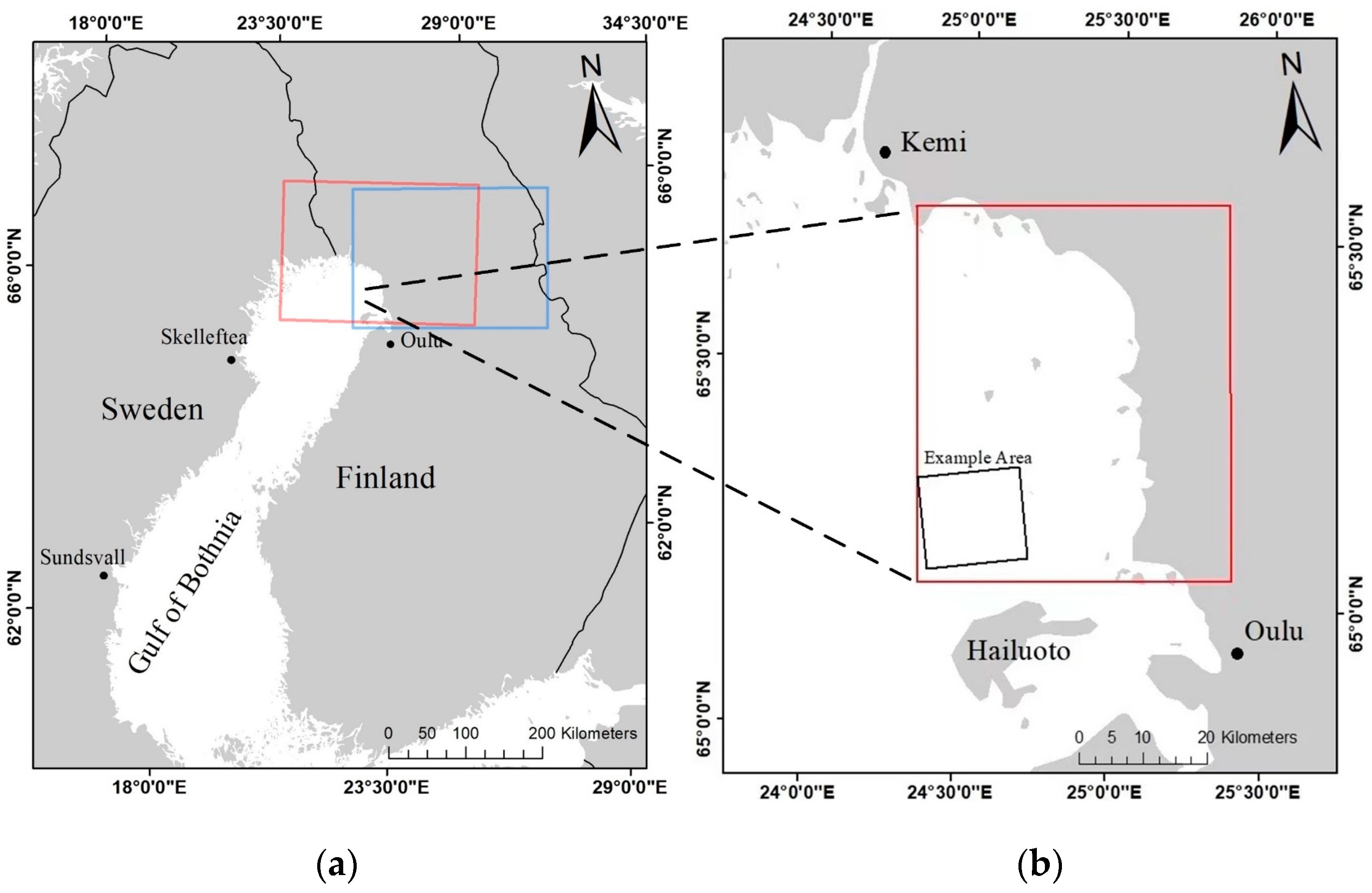
2.1. Study Area

The Baltic Sea, an inland sea in northern Europe, is one of the largest brackish water areas in the world. The sea ice in the Baltic Sea usually occurs in the shallow coastal area of the northernmost part of the Gulf of Bothnia in November each year. Maximum coverage is reached in February or March of the following year [28]. In the Gulf of Bothnian, the average annual fast ice thickness is usually 0.58 ± 0.13 m [29]. Then the sea ice usually lasts until mid-May before melting. Although the seasonal ice cover of the Baltic Sea has many similarities to that of the Polar oceans, it has many unique characteristics, which are mainly caused by the brackish water that forms the ice, resulting in low salinity per unit volume and porosities. In addition, the maximum ice extent in the Baltic Sea varies greatly from year to year because of the milder climate in this area than in the Polar regions. Rainfall and freeze–thaw cycles can occur throughout the winter [30]. As trade increases, there is a growing need for ice transportation in winter. Although landfast ice provides convenience in transportation, it also brings many environmental problems. The interaction between landfast ice and land causes the erosion of the shore and sea bottom [31]. Therefore, it is of great significance to study the local landfast ice to avoid sea ice disasters and serve winter transportation. As shown in Figure 1b, the northeastern coast of the Gulf of Bothnia (24.5–25.5° E, 65.0–65.6° N) located in the northern Baltic Sea is selected as the study area. The characteristics of high latitude and long glacial period here are particularly suitable for the study of landfast ice.

In two previous studies in the study area [20,23], X-band SAR of the Italian Cosmo-Sky Med constellation and C-band SAR of ERS-1 were used to detect landfast ice, with a temporal baseline of 1 day and 3 days, respectively. These SAR data with short temporal baselines tend to be more suitable for the detection of small displacements. Recently, a study on the Baltic Sea successfully obtained the landfast ice extent using C-band SAR of Sentinel-1 [27]. The authors have demonstrated that the potential of Sentinel-1 data to detect landfast ice with a temporal baseline of 12 days and indicated the advantage of a long temporal baseline in separating fast ice from the drifting ice. Unfortunately, the study did not consider the details of landfast ice edge as it mainly focused on ice displacement. In a similar research in the Arctic [9], L-band SAR of ALOS was used to extract landfast ice edge with a longer temporal baseline of 46 days as the fast ice in this region is more stable than that in the Baltic Sea. Generally, one of the main limitations of InSAR technology in application is the temporal decorrelation of the SAR signals. Based on the previous works, this paper develops a modified approach of extracting landfast ice edge and focuses on its performance in extracting landfast ice edge using Sentinel-1 data.

2.2. Data

In this paper, four InSAR image pairs constructed by eight Sentinel-1A SLC (Single Look Complex) data acquired from July 2018 to February 2019 are used to extract landfast ice along the coast of the Gulf of Bothnia. C-band used by Sentinel-1A is considered to be a relatively compromised band in sea ice detection. Compared with the L-band, it has more advantages in the comparison of sea ice of different ages [32]. As shown in Figure 1a, the Sentinel-1A data acquired from two different orbits covering the study area are used. A two-orbit coverage provides more data than one-orbit coverage in the same period. Hence, it is possible to obtain the image pairs of the same area in less than 12 days, which improves the temporal resolution of landfast ice observation. The specific information of Sentinel-1A data is shown in

Table 1. Characteristics of Sentinel-1A image pairs.

No.	Master Image	Slave Image	Orbit Number	Temporal Baseline/Day	Spatial Baseline/m	Product Type	Pass Direction	Polarization
1	20/07/2018 *	01/08/2018	51	12	11.225	SLC	descending	VV/VH
2	18/12/2018	30/12/2018	153	12	7.912	SLC	descending	VV/VH
3	16/01/2019	28/01/2019	51	12	33.522	SLC	descending	VV/VH
4	23/01/2019	04/02/2019	153	12	25.198	SLC	descending	VV/VH

* Format: day/month/year.

. Moreover, the ACE2 (Altimeter Corrected Elevations, Version 2) DEM released by NASA (National Aeronautics and Space Administration) is applied to InSAR data processing in this study [33].

2.3. Validation Data

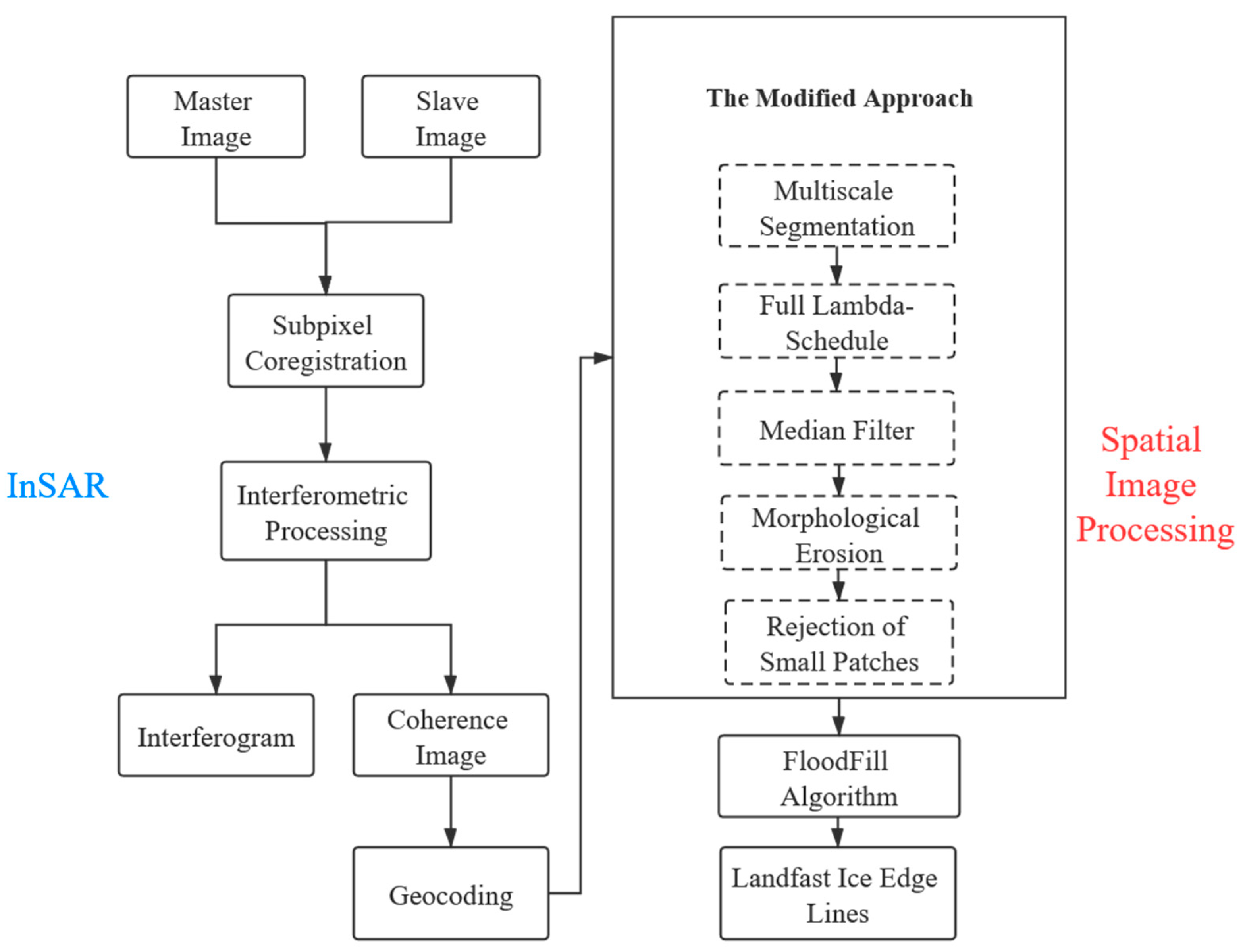
The daily ice charts [34] published by the Swedish Meteorological and Hydrological Institute (SMHI) and the global coastline data [35] released by the National Oceanic and Atmospheric Administration (NOAA) are used as the reference data to validate the accuracy of the results of landfast ice edge. The daily ice charts provide detailed information about the types, thickness and coverage of sea ice in the Baltic Sea throughout the whole year. Ice analysts from the SMHI use the latest available Earth observation (EO) data, mainly SAR images, and in-situ data for producing the ice charts [17]. SAR images as the base for most ice charts are manually interpreted by experienced analysts. The in-situ data originate from Finnish and Swedish icebreakers, coastal ice observation stations of the Baltic Sea ice services, and other occasional sources.

3. Methods

The reference [9] has completely presented a method to extract landfast ice edge from InSAR data, which can be used as a reference method in this paper. Based on the processing flow of the reference method, this paper introduces a modified approach to extract the landfast ice edge and illustrates its performance relative to the reference method. The methodology workflow is shown in Figure 2. InSAR provides basic images for the intuitive interpretation of landfast ice. The proposed approach is a four-step procedure mainly including image multiscale segmentation, median filter, morphological erosion, and rejection of small patches, which is used to accurately obtain landfast ice edge.

3.1. InSAR Processing and Concepts

The fundamentals of InSAR technology can be found in reference [7,23]. InSAR is a technology that measures phase differences between two SAR images acquired from two similar viewing geometries [22]. The phase difference after coregistration can be used to measure topography and terrain displacement [27]. The InSAR processing generally includes image coregistration, interferogram generation, coherence image generation, flat earth removal, interferogram filtering, low-coherence area mask, phase unwrapping, and phase-to-height conversion [7,36]. All the aforementioned steps can be carried out with the Sentinel’s Application Platform (SNAP) software.

In this paper, an interferometric image pair is constructed by two Sentinel-1 SAR images (the one with an earlier acquisition time, used as a geometric reference, will be called the “master image” and the other the “slave image”) from different acquisition times. The SNAP software is used for processing the satellite SAR data to generate and geocode the coherence image. Then, the coherence image is geocoded to transfer the SAR image coordinate system to the geographic coordinate system (WGS_1984_UTM_Zone_34N) for subsequent processing. Over the geocoded coherence image, the edge between landfast ice and drifting ice is extracted by the modified approach. Finally, the full landfast ice extent is obtained using floodfill algorithm.

3.2. Coherence Image

Coherence (ranging between 0 and 1) is a measure of the quality of the interferogram, which is high if scatterers remain unchanged and low if there is significant change in the scattering medium [22]. The complex coherence between two complex SAR images ${\mu }_1$ and ${\mu }_2$ is defined as [9]:

$$\gamma =\frac{E[{\mu }_1{\mu }_2^{*}]}{\sqrt{E[{|{\mu }_1|}^2]E[{|{\mu }_2|}^2]}}$$

(1)

where E[.] is the mathematical expectation, and ${\mu }^{*}$ is a conjugate complex. Based on the definition, in the actual InSAR calculation, the coherence of the real data is calculated according to Formula (2), which is transformed from Formula (1):

$$\gamma =\frac{{{\displaystyle \sum }}_{n=1}^N{{\displaystyle \sum }}_{m=1}^M{\mu }_1\left(n,m\right){\mu }_2^{*}\left(n,m\right)}{\sqrt{{{\displaystyle \sum }}_{n=1}^N{{\displaystyle \sum }}_{m=1}^M{|{\mu }_1\left(n,m\right)|}^2{{\displaystyle \sum }}_{n=1}^N{{\displaystyle \sum }}_{m=1}^M{|{\mu }_2\left(n,m\right)|}^2}}$$

(2)

where M and N are the sizes of the moving window for calculating the coherence; n and m are the row and column numbers in the window; ${\mu }_1$(n,m) and ${\mu }_{2 }$(n,m) are the complex values at the image coordinates (n,m), respectively; |.|² is the 2-norm of the data. Here, a 10 × 3 window in range and azimuth is applied to estimate the coherence.

The coherence value indicates the stability and correlation of the land features between two acquisitions. The displacement and deformation of landfast ice are usually small owing to its stable ice body, so its coherence is relatively high. But for drifting ice or water, its coherence is relatively low due to the influences of strong winds and changing ocean currents. Ocean currents will constantly change the distribution of drifting ice and may break up its body with high energy [37]. Therefore, the difference between landfast ice and drifting ice in coherence provides an obvious discrimination (bright and dark) in coherence image.

3.3. Approach to Landfast Ice Edge Extraction

The reference method provides a processing chain that combines a statistical CFAR (constant false alarm rate) classification with spatial image processing steps. The final landfast ice edge is obtained based on the following six steps: statistical coherence thresholding, morphological image analysis, image segmentation, patch size analysis, final morphological closing procedure, and outline extraction. In this paper, a modified approach with four steps is proposed to preserve more features of landfast ice edge.

The first step of the modified approach is image segmentation. Although the difference between drifting ice and landfast ice is quite obvious in coherence image, they still share a common coherence range. Hence, a simple pixel-based threshold operator will lead to misclassifications of pixels whose coherence values are close to the detection threshold. Moreover, due to the influence of speckle noise, it is difficult to obtain continuous high coherence region if the pixel is the unit of processing [38]. Therefore, the coherence image should be segmented first, and the subsequent processing should be based on the segmentation units. In view of the above, an object-oriented multiscale segmentation algorithm [39] is used for coherence image. This algorithm analyzes the multiscale properties of watershed boundaries and gradient watershed boundaries for an image which can provide better results in edge detection [40]. More details of this algorithm can be found in reference [40,41]. In this paper, the Sobel operator (an edge operator) is used to calculate gradient values and generate gradient image. After obtaining the gradient image, quantization ranges can be created by Formula (3) to calculate a cumulative relative histogram:

$$Q_{quant\_levels}=V_{min}+\left(\left(quant\_levels\right)\ast \left(V_{max}-V_{min}\right)\right)/\left(quant\_levels\right)$$

(3)

where quant_levels is a specified value representing the number of unique levels. V_min and V_max represent the minimum and maximum values of the data, respectively. The histogram can be used along with the gradient image to calculate the gradient scale-space. Once the scale is selected, the gradient image is modified so that the pixels with gradient magnitude less than the gradient threshold are set to have the same value with the gradient threshold. Then watershed transformation is applied on the modified gradient image to obtain multiscale segmentation result for the whole image.

To deal with over-segmentation, the Full Lambda-Schedule algorithm proposed by Redding et al. [42] is used as the merging model. This algorithm merges adjacent small patches by combining spectral and spatial information iteratively. For two adjacent regions O_i and O_j, when the merging condition t_i,j is less than the threshold λ, the two regions are merged into one. The formula for the merging condition t_i,j is as follows:

$$t_{i,j}=\frac{\frac{|O_i||O_j|}{|O_i|+|O_j|}\Vert u_i-u_j\Vert {}^2}{l\left(\partial \left(O_i,O_j\right)\right)}$$

(4)

where |O_i| and |O_j| denote the areas of O_i and O_j, respectively; u_i and u_j are the mean values of O_i and O_j; ‖u_i − u_j‖ denotes the Euclidean distance between the mean value of O_i and O_i, l(∂(O_i,O_j)) denotes the length of the common boundary of O_i and O_j. A threshold segmentation is then ready to operate for the multiscale segmented image. The image is divided into three sub-regions before threshold segmentation: drifting ice, landfast ice, and land. Then the mean coherence values of the three sub-regions are determined based on selecting random samples. Finally, the threshold segmentation can be operated according to the Mode method [43].

The second step of the approach is a median filter. Due to noise and other factors, isolated patches with high coherence will remain outside the main landfast ice in the segmented image. Hence, a filter that can remove small patches but also preserve edge is necessary before the next step. Here, a median filtering with a window of 3 × 3 is used on the image.

The third step is morphological erosion. The function of morphological erosion is to further remove the patches and shrink to form edge. For a binary image, A and B are two sets, in 2D integer space Z², eroding the set A by structuring elements of B is defined as [44]:

$$\left(\mathrm{A}\mathsf{\Theta }\mathrm{B}\right)=\left\{\mathrm{Z}|{\left(\mathrm{B}\right)}_{\mathrm{Z}}\subseteq \mathrm{A}\right\}$$

(5)

A new set is created by running B over set A so that the origin of B visits every element of the set A. Therefore, at each location of the origin of the structuring elements of B, if B is completely contained in the set A, then the element for that location (where the origin of the structuring element B lays) is marked as a member of the new set.

The fourth step of the approach is a rejection of small patches. Although the median filter and morphological erosion both have the ability to remove small patches, they cannot deal with the patches or floating fast ice outside the main body whose size are larger than their processing window. Therefore, the remaining patches with high coherence are completely removed by setting an area threshold.

The initial segmentation also leaves low-coherence holes in the land and landfast ice. If trying morphological dilation repeatedly to fix these holes, it will cause a blurred edge and feature loss. At the same time, additional operations are still required because only a portion of the holes can be fixed. As this study focuses on the clear edge of landfast ice, holes in the main body are of less importance. Thus, the holes are fixed as fast ice based on the floodfill algorithm [45]. After all these steps, the landfast ice edge is obtained eventually.

The most distinctive feature by which this modified approach differs from the reference method is in the detection and preservation of the landfast ice edge. The edge result is obtained from the optimal segmentation between multiscale gradient images. Compared with edge extraction under one certain scale, this result contains more information about edge. In addition, all the latter steps after image segmentation are considered to avoid the loss of edge feature. The median filter in the second step is an edge-preserving filter. In fixing the inside holes, the routine operation in the reference method uses the morphological dilation. However, it is replaced with floodfill algorithm for preserving the edge and fixing all holes.

The edge extraction is usually aimed at the seaward landfast ice edge. For the landward edge, the existing coastline data is generally used to replace it. However, the coastline changes year by year in coastal areas severely eroded by fast ice [46]. Inaccurate results can be caused by using low-resolution or untimely updated coastline data. This study adds the work of extracting landward landfast ice edge and validates the performance of the modified approach. Sentinel-1A provides a large amount of available data given its high spatial resolution and temporal coverage. Thereby, Sentinel-1A data from the summer ice-free period of the observation year are used to construct the image pair. The difference in coherence between land and sea surface can be used to extract the land–water boundary as the landward edge of landfast ice through the same technical method.

4. Results

The main research results include coherence images, intermediate processing results of landfast ice edge extraction, and edge line maps. Section 4.1 shows the coherence image obtained by the InSAR and the intermediate results by the modified approach. Section 4.2 shows the landfast ice edge obtained by the reference method and modified approach on coherence images.

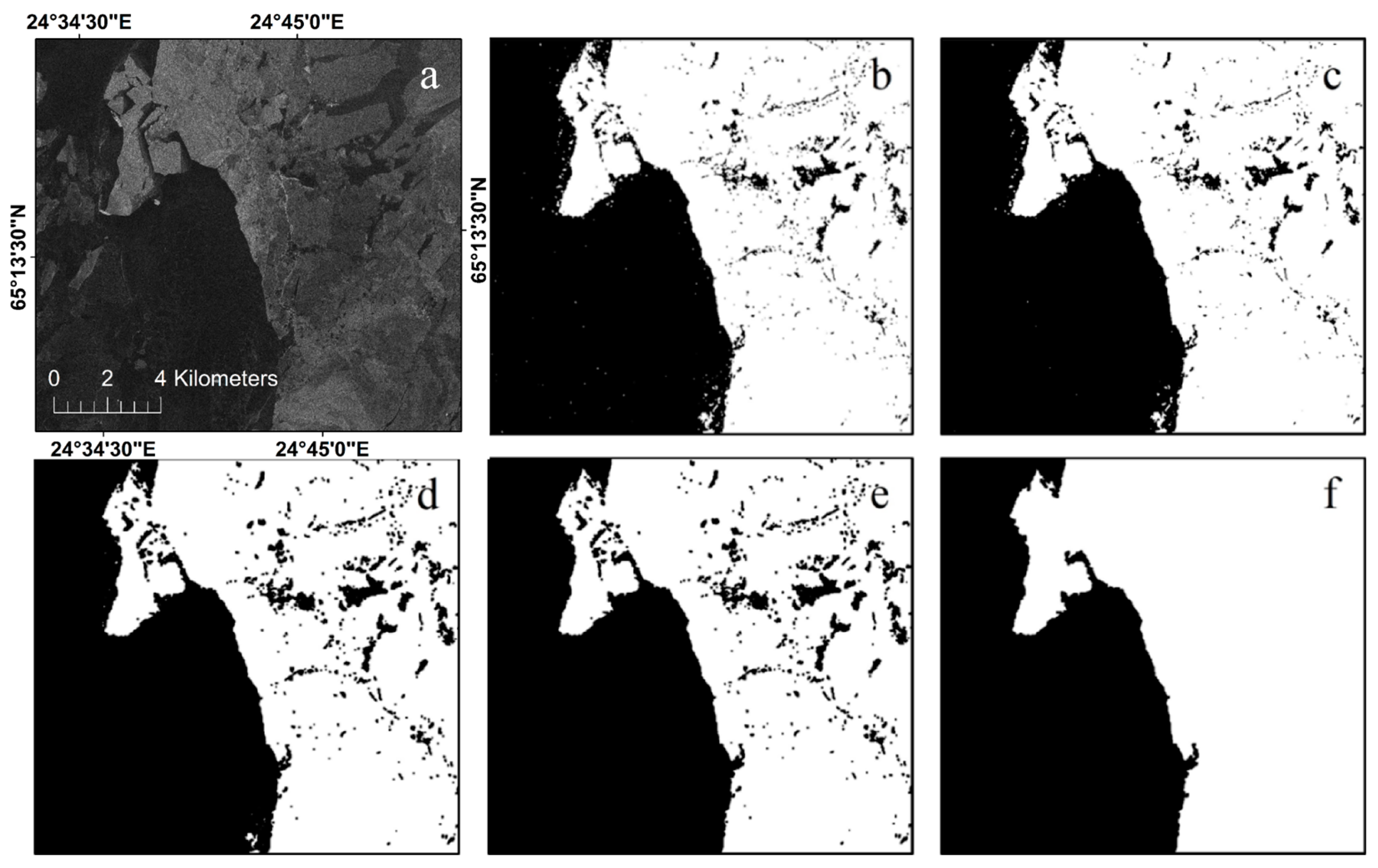
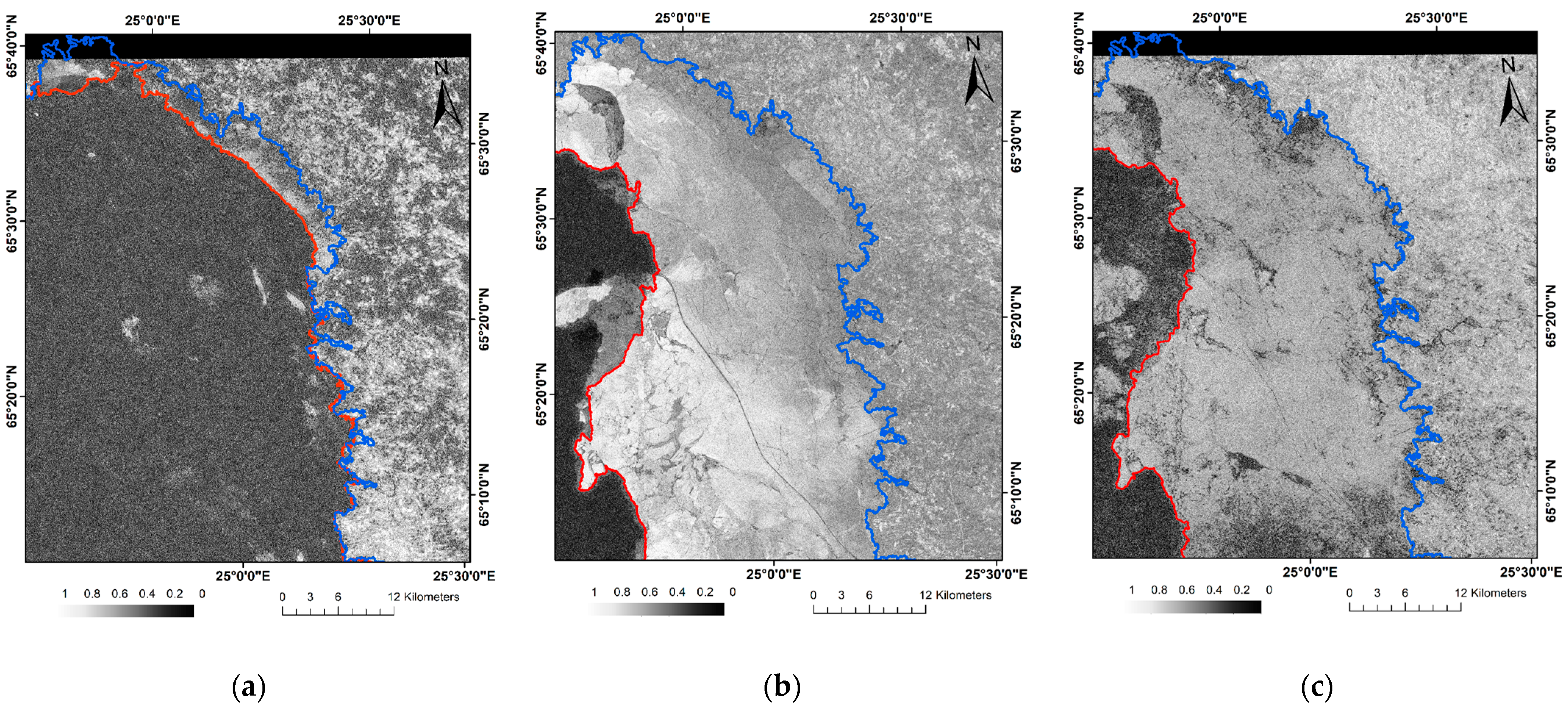
4.1. Coherence Image and Intermediate Processing Results

The coherence image of the example area is shown in Figure 3a, where the grayscale of coherence image indicates the stability and correlation of sea ice during the interval time when the image pair is acquired. Figure 3b–f shows the edge extraction process based on the modified approach. The isolated high-coherence patches are removed after median filtering, morphological erosion, and rejection of small patches in sequence (Figure 3c–e). The holes with low coherence are fixed by floodfill algorithm (Figure 3f).

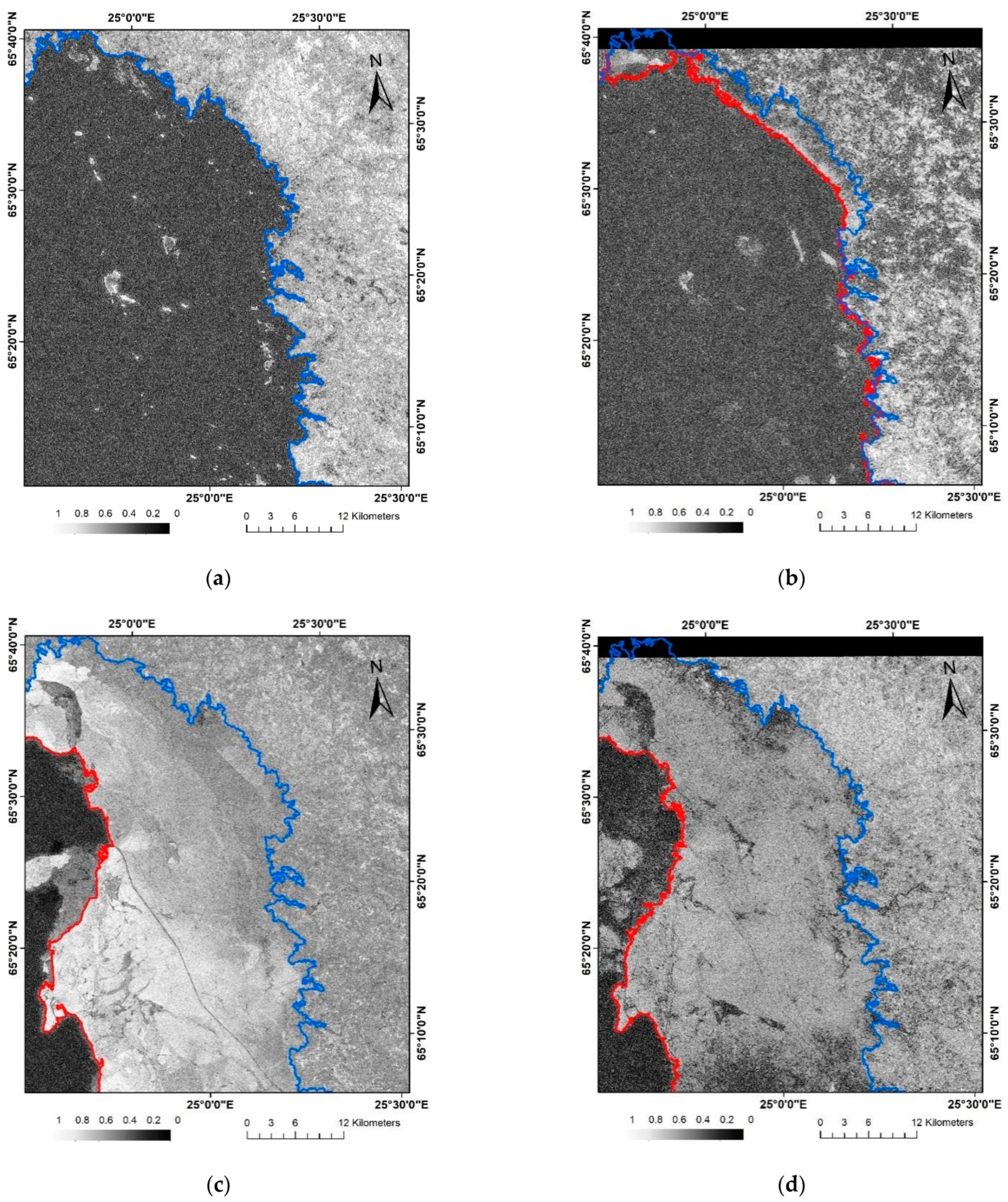
4.2. Landfast Ice Edge Line Maps

Four image pairs are used to extract three seaward edge lines of landfast ice at different times and one land-water boundary in ice-free summer. The image pairs used are shown in

Table 2. Statistical parameters of segments.

Statistical Parameters	Value (km2)
Minimum	−0.66
Maximum	0.61
Mean	0.00
Standard Deviation	0.07
Sum Positive	4.40
Sum Negative	−3.04
Number of segments (only area > 0.1 km2)	12

. Figure 4 and Figure 5 show the edge line maps of landfast ice obtained by modified approach and reference method, respectively. The red curves are the seaward edge lines of landfast ice, and the blue curve is the land–water boundary.

5. Discussions and Analysis

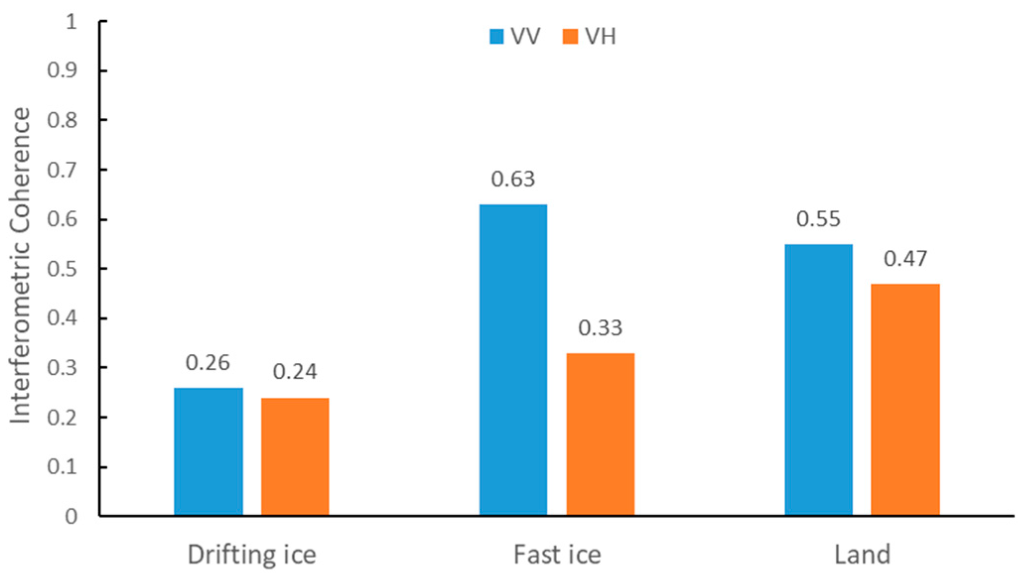
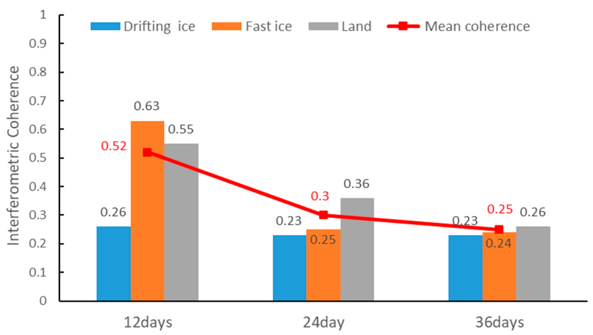
5.1. Coherence under Different Conditions

The Sentinel-1A IW data contain two polarization modes: VV polarization and VH polarization. Different polarization modes have different responses to features. Taking the image pair 3 (see Table 1) as an example, image pairs under VV and VH polarization are constructed respectively to study the impact of different polarization modes on edge extraction. It can be seen from the coherence statistics (Figure 6) that, under VV polarization, the mean coherence value of landfast ice is 0.63, whereas that of drifting ice is 0.26, and the difference between them is 0.37. Under VH polarization, the mean coherence value of landfast ice is 0.33, whereas that of drifting ice is 0.24, and their difference is only 0.09. Therefore, the divisibility between different objects is higher under VV polarization. Since the co-polarization of the C-band is more sensitive to the dielectric constant and surface roughness of objects than cross-polarization [47] and the landfast ice edge under VV polarization is clearer than that under VH polarization, further analysis concentrates on the VV polarization mode.

In InSAR technology, the temporal baseline of image pairs determines how long sea ice remains stationary before it can be classified as fast ice. To select the appropriate temporal baseline, image pairs with different temporal baselines are constructed in the study area, and then coherence statistics is performed. As shown in Figure 7, the overall mean coherence gradually decreases as the time interval of the temporal baseline increases. Under the temporal baseline of 12 days, the mean coherence values of fast ice and drifting ice are 0.63 and 0.26, respectively, and their difference is up to 0.37. When the temporal baseline is increased to 24 days and 36 days, the coherence difference between the fast ice and drifting ice is only 0.02 and 0.01, respectively, which can no longer meet the requirements of extracting landfast ice edge. The ice charts show that the thickness of sea ice increases from 10–30 cm to 40–55 cm within 36 days. Influenced by temporal de-coherence factors, severe de-coherence phenomenon can occur when sea ice changes significantly. In theory, the longer the temporal baseline is used, the more accurate the landfast ice extent is obtained. But the longer baseline also means an increased probability of de-coherence. It is the best solution to select the longest temporal baseline considering the available coherence images, so the temporal baseline in this paper is 12 days.

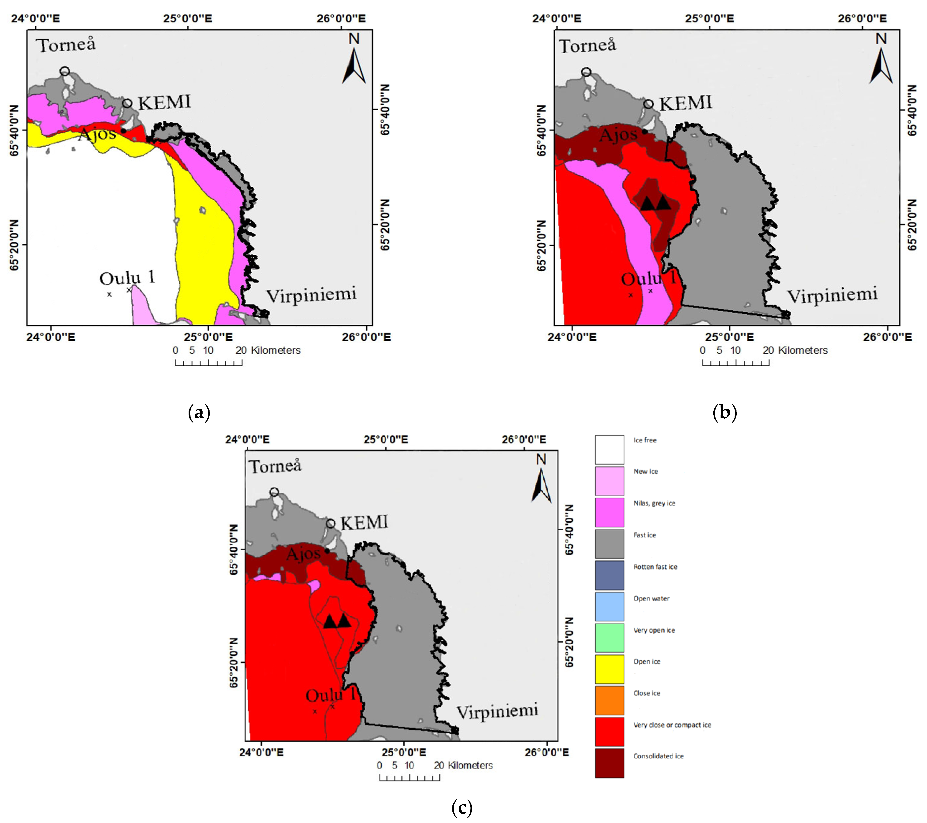
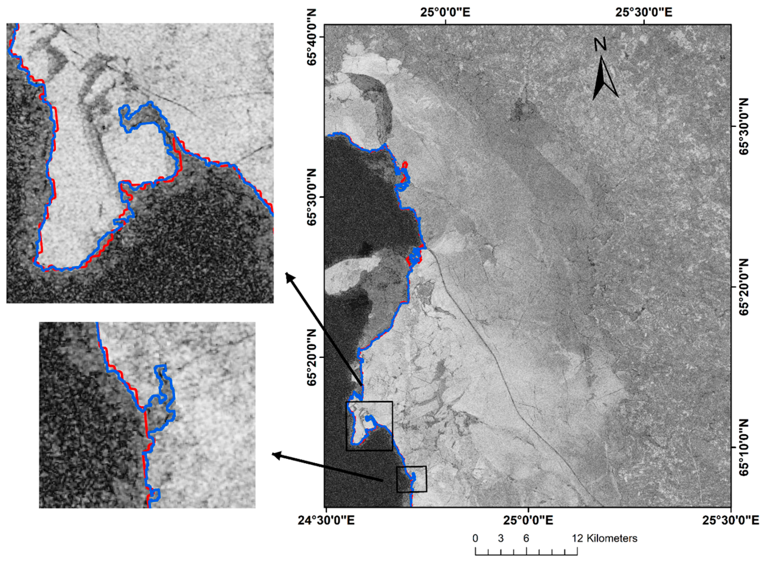
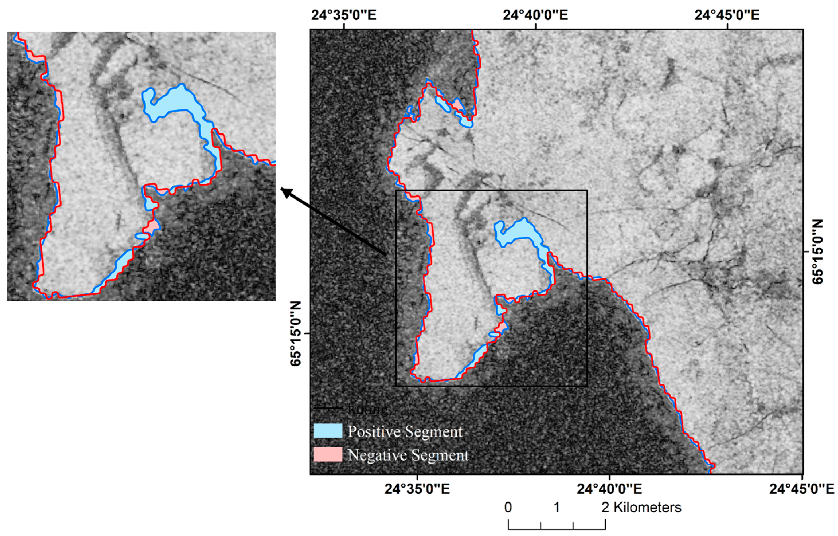
5.2. Verification of Landfast Ice Edge

For evaluating the extracted seaward landfast ice edge, ice charts published by SMHI are used for verification. Daily ice charts are easily available on the SMHI website. The primary publication format of the ice chart is a PDF product, so the vector form of landfast ice extent is not available in this product. Nonetheless, these charts still can be roughly geocoded by their latitudes and longitudes. After geocoding, ice charts and landfast ice edge are shown in the same geographic coordinate system for direct visual comparison. It is noted that this is only a rough comparison. The main purpose is to validate the overall shape and distribution, not the precision of landfast ice edge.

The results are shown in Figure 8. The seaward landfast ice edge extracted in this paper are generally consistent with those in ice charts. Because of high resolution of Sentinel-1A, the edge lines show more details in the results. All the three results of seaward landfast ice edge from different periods provide consistent results with ice charts, confirming the potential of the method in monitoring the changes of landfast ice extent. However, some differences are observed in a few regions. One reason is that the edge of the landfast ice must be simplified to cater to the rough scale when drawing ice charts. In addition, since the definition adopted in this paper is similar to that proposed by Mahoney et al., landfast ice is defined as is contiguous with the coastline and remains stationary over a 12-day time period in consecutive images. This difference can be explained by the ice chart preparation process where the ice analysts tend to avoid overestimating the expansion of the landfast ice by consolidated ice in order to indicate probable wind-induced break-off zones and that way to diminish risks caused by rapid day-to-day changes [17].

This paper also gives the result about the distance that landfast ice edge move from one image pair to the next. From image pair 2 to image pair 3, landfast ice edge moves about 19.9 km, as more sea ice becomes stable. From image pair 3 to image pair 4, landfast ice edge is nearly unmoved. This is probably because the ice conditions are stable during a short-time observation.

Ice charts are only used to roughly verify the extent and changes of landfast ice due to lack of precise vector data. In order to further illustrate the performance of the modified approach, a comparison with the reference method is provided below. This comparison is carried out on the same coherence image from image pair 3. Figure 9 shows the comparison process of the two methods. The visual interpretation indicates that these two methods provide very approximative results with landfast ice edge, thus proving the applicability of the modified approach. The main difference between the two methods is the elaboration degree in landfast ice edge. From two cases in Figure 9, the edge of reference method is coarser without many features. These features are replaced with a simple line because of the edge distortion caused by the processing of the reference method. On the contrary, these edge features are preserved in the result of the modified approach.

For quantitative comparison, an area analysis of relative extraction difference is performed. The result is shown in Figure 10. The area differences of extracted landfast ice are described by many positive and negative segments. Negative (in red) segments indicate relative underestimation by the reference method while positive (in blue) segments indicate a relative underestimation of landfast ice extent by the modified approach. The statistical analysis of these segments in Table 2 shows that the two methods provide very close results with landfast ice area differing by only 1.36 km² over a coastline length of 345 km. Moreover, the segments have a low value in mean, standard deviation and number of segments, indicating the stability of the modified approach in extracting landfast ice. In brief, the modified approach not only has a satisfying segmentation effect on the whole image, but also preserves more details in local edge. It is confirmed that the modified approach is suitable for extracting landfast ice edge.

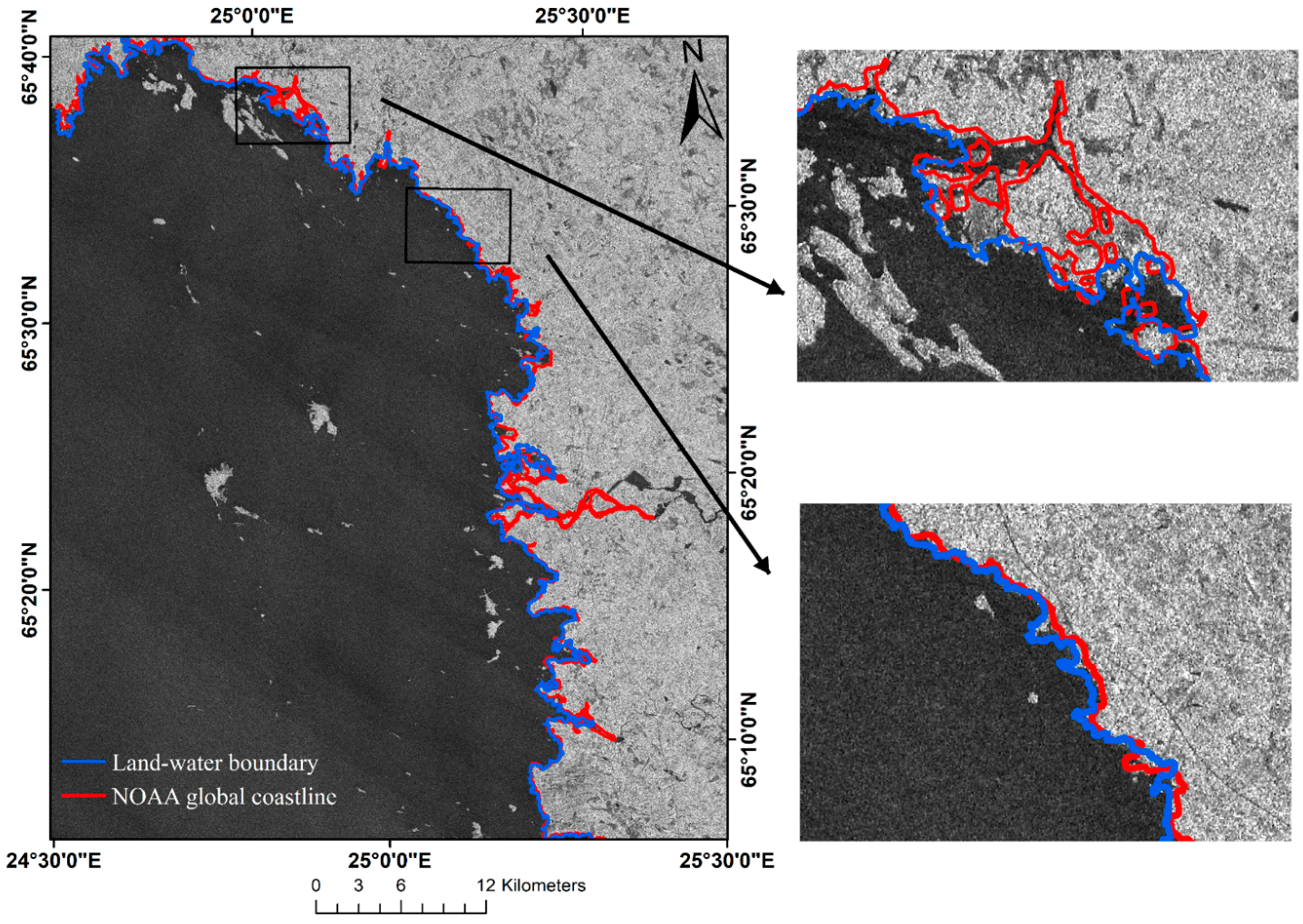
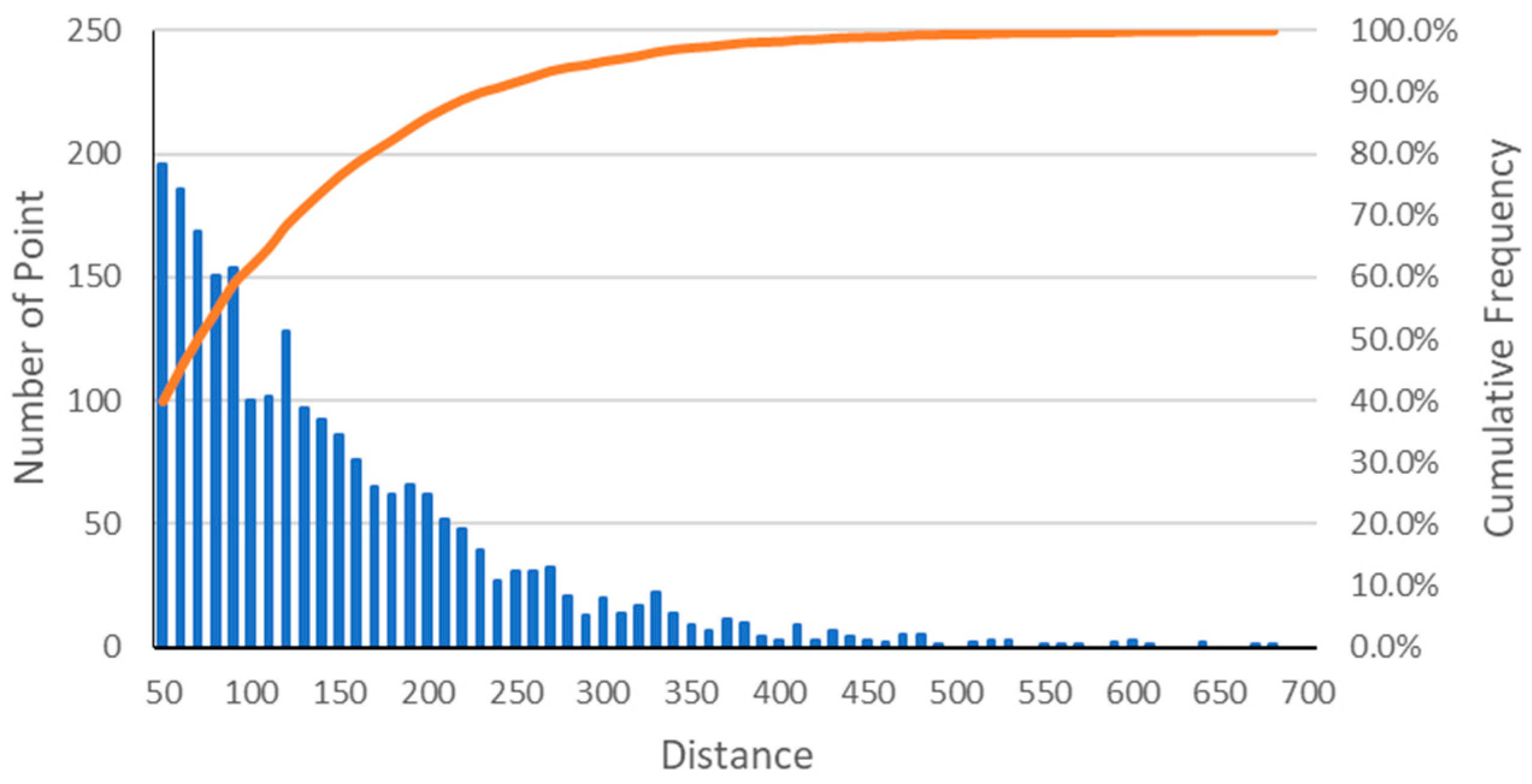
5.3. Verification of the Land–Water Boundary

The land–water boundary extracted by image pair 1 is compared with the global coastline data released by NOAA to evaluate the performance of the method proposed in this study.

Figure 11 shows the comparison process of the land–water boundary. The two results provide a similar display on the whole area, which are consistent with the actual terrain without large deviations. Either of them meets the need for coastline mapping. Specifically, in a large area where the coastline is relatively straight, the land–water boundary is better than the coastline data and is closer to the actual topography. While in a small area with many offshore islands and a tortuous coastline, more islands close to the coast and main rivers entering the sea are mapped in the coastline data. As a result, the NOAA global coastline is better than the land–water boundary here.

Similarly, statistical parameters of distance from the land–water boundary to the NOAA global coastline are calculated as shown in

Table 3. Statistical parameters of the land–water boundary.

Statistical Parameters	Value (m)
Minimum	0
Maximum	684.5
Mean	109.1
Standard Deviation	99.8

. And a frequency histogram of sampling points (Figure 12) is generated to analyze the distance distribution. The statistical results show that over the 345 km long coastline, the mean distance from the land-water boundary to the coastline data is 109.1 m, the standard deviation is 99.8 m, and 84% of the sampling points are within 200 m. The validation of results illustrates the stability and reliability of the method used in the mapping tasks of the land–water boundary.

5.4. Comparison with SAR-Based Methods

In this paper, landfast ice edge is extracted based on the coherence images. Rather than SAR amplitude image, the coherence image can be used to detect the movement trend of sea ice within 12 days and distinguish the moving drifting ice from the stationary ice. SAR-based methods generally need sufficient textures in SAR images. However, sea ice textures have different electromagnetic interaction behaviors and gray levels, which may result in misinterpreted observations and imprecise SAR classifications [48].

As shown in the SAR amplitude image (Figure 13), regardless of VV polarization or VH polarization, thin sea ice exhibits high variability in backscatter magnitude and polarization difference, making it difficult to distinguish it from open water and fast ice [49]. The high sensitivity of sea ice to the incidence angle leads to complex changes in backscatter magnitude between different types and even in the same type of sea ice [50]. Subtraction and cross-correlation of colocated image pairs will not yield accurate results unless a coastal flaw lead between the landfast and drifting ice is present. Therefore, a single amplitude image is insufficient to identify the boundary of the fast ice. The amplitude image contains substantial information about the features, and it has many advantages in sea ice classification. When only focusing on fast ice though, using the coherence image can be convenient and reliable to quickly distinguish the fast ice from other types of sea ice.

6. Conclusions

In this paper, the landfast ice edge in northernmost Gulf of Bothnia is extracted using InSAR technology with the image pairs of Sentinel-1A. With the interferometric coherence image, a modified approach of extracting the landfast ice edge based on multiscale segmentation and morphological erosion is proposed. This approach takes the advantages of interferometric coherence and multiscale behavior of edge to distinguish the fast ice from drifting ice. As a result, the seaward landfast ice edge and land–water boundary are successfully obtained. Through this study, some important conclusions can be drawn as follows:

(1)

Based on InSAR technology, the landfast ice edge can be detected with high accuracy. The interferometric image pair with VV polarization and the temporal baseline of 12 days can help extract landfast ice edge and achieve a balance between coherence and accuracy.

(2)

Over a coastline length of 345 km in the study area, the difference in area between landfast ice obtained by the modified approach and reference method is only 1.36 km². The mean distance between the land–water boundary and the reference coastline released by NOAA is 109.1 m, and the standard deviation is 99.8 m. Compared with other methods, the method proposed in this paper performs well in terms of stability and accuracy. It also provides more details about the local landfast ice edge.

(3)

During the observation period (December 2018–January 2019), three landfast ice edge line maps are successfully obtained. The area of landfast ice are 170.2 km², 1447.2 km², and 1450.4 km² in the three periods. The results demonstrate the potential of the proposed method in monitoring the landfast ice extent and studying the changes of fast ice.

Since the extraction of landfast ice edge still falls under InSAR-based methods, the choice of the temporal baseline is limited by the satellite revisit cycle and the coherence will be influenced by de-coherence factors. When constructing the image pairs, one needs to consider the changes that may occur in the sea ice. This paper presented a method to extract landfast ice edge when the coherence image is available. With following radar system plans in the future, the improvement of multi-band, multi-sensor, and short revisit cycle will provide more potential and possibilities for the research of landfast ice.

References

1. Giles, A.B.; Massom, R.A.; Lytle, V.I. Fast-ice distribution in East Antarctica during 1997 and 1999 determined using RADARSAT data. J. Geophys. Res.-Oceans 2008, 113, C02S14. [Google Scholar] [CrossRef] [Green Version]
2. Dammann, D.O.; Eicken, H.; Meyer, F.J.; Mahoney, A.R. Assessing small-scale deformation and stability of landfast sea ice on seasonal timescales through L-band SAR interferometry and inverse modeling. Remote Sens. Environ. 2016, 187, 492–504. [Google Scholar] [CrossRef] [Green Version]
3. Kiani, S.; Irannezhad, M.; Ronkanen, A.K.; Moradkhani, H.; Kløve, B. Effects of recent temperature variability and warming on the Oulu-Hailuoto ice road season in the northern Baltic Sea. Cold Reg. Sci. Tech. 2018, 151, 1–8. [Google Scholar] [CrossRef] [Green Version]
4. Lund-Hansen, L.C.; Petersen, C.M.; Søgaard, D.H.; Sorrell, B.K. A Comparison of Decimeter Scale Variations of Physical and Photobiological Parameters in a Late Winter First-Year Sea Ice in Southwest Greenland. J. Mar. Sci. Eng. 2021, 9, 60. [Google Scholar] [CrossRef]
5. Eicken, H.; Lovecraft, A.L.; Druckenmiller, M.L. Sea-ice system services: A framework to help identify and meet information needs relevant for arctic observing networks. Arctic 2009, 62, 119–136. [Google Scholar] [CrossRef] [Green Version]
6. Timco, G.W.; Weeks, W.F. A review of the engineering properties of sea ice. Cold Reg. Sci. Tech. 2010, 60, 107–129. [Google Scholar] [CrossRef]
7. Huang, L.; Hajnsek, I. Polarimetric Behavior for the Derivation of Sea Ice Topographic Height From TanDEM-X Interferometric SAR Data. IEEE J. Sel. Top. Appl. Earth Observ. Remote Sens. 2020, 14, 1095–1110. [Google Scholar] [CrossRef]
8. Keller, M.R.; Gifford, C.M.; Winstead, N.S.; Walton, W.C.; Dietz, J.E. Active/Passive Multiple Polarization Sea Ice Detection During Initial Freeze-Up. IEEE Trans. Geosci. Remote Sens. 2020, 59, 5434–5448. [Google Scholar] [CrossRef]
9. Meyer, F.J.; Mahoney, A.R.; Eicken, H.; Denny, C.L.; Druckenmiller, H.C.; Hendricks, S. Mapping arctic landfast ice extent using L-band synthetic aperture radar interferometry. Remote Sens. Environ. 2011, 115, 3029–3043. [Google Scholar] [CrossRef]
10. Mahoney, A.; Eicken, H.; Graves, A.; Shapiro, L. Defining and locating the seaward landfast ice edge in northern Alaska. In Proceedings of the 18th International Conference on Port and Ocean Engineering under Arctic Conditions, Potsdam, NY, USA, 26–30 June 2005; Volume 3, pp. 991–1001. [Google Scholar]
11. Fraser, A.D.; Massom, R.A.; Michael, K.J. Generation of high-resolution East Antarctic landfast sea-ice maps from cloud-free MODIS satellite composite imagery. Remote Sens. Environ. 2010, 114, 2888–2896. [Google Scholar] [CrossRef]
12. Li, X.; Ouyang, L.; Hui, F.; Cheng, X.; Shokr, M.; Heil, P. An improved automated method to detect landfast ice edge off Zhongshan Station using SAR imagery. IEEE J. Sel. Top. Appl. Earth Observ. Remote Sens. 2018, 11, 4737–4746. [Google Scholar] [CrossRef]
13. Dammann, D.O.; Eriksson, L.E.B.; Mahoney, A.R.; Eicken, H.; Meyer, F.J. Mapping pan-Arctic landfast sea ice stability using Sentinel-1 interferometry. Cryosphere 2019, 13, 557–577. [Google Scholar] [CrossRef] [Green Version]
14. Dierking, W.; Lang, O.; Busche, T. Sea ice local surface topography from single-pass satellite InSAR measurements: A feasibility study. Cryosphere 2017, 11, 1967–1985. [Google Scholar] [CrossRef] [Green Version]
15. Karvonen, J. Estimation of Arctic land-fast ice cover based on dual-polarized Sentinel-1 SAR imagery. Cryosphere 2018, 12, 2595–2607. [Google Scholar] [CrossRef] [Green Version]
16. Dammann, D.O.; Eicken, H.; Mahoney, A.R.; Saiet, E.; Meyer, F.J.; John, C. Traversing sea ice—linking surface roughness and ice trafficability through SAR polarimetry and interferometry. IEEE J. Sel. Top. Appl. Earth Observ. Remote Sens. 2017, 11, 416–433. [Google Scholar] [CrossRef]
17. Mäkynen, M.; Karvonen, J.; Cheng, B.; Hiltunen, M.; Eriksson, P.B. Operational Service for Mapping the Baltic Sea Landfast Ice Properties. Remote Sens. 2020, 12, 4032. [Google Scholar] [CrossRef]
18. Mahoney, A.; Eicken, H.; Gaylord, A.G.; Gens, R. Landfastsea ice extent in the Chukchi and Beaufort Seas: The annual cycle and decadal variability. Cold Reg. Sci. Technol. 2014, 103, 41–56. [Google Scholar] [CrossRef]
19. Dammann, D.O.; Eicken, H.; Mahoney, A.R.; Meyer, F.J.; Freymueller, J.T.; Kaufman, A.M. Evaluating landfast sea ice stress and fracture in support of operations on sea ice using SAR interferometry. Cold Reg. Sci. Technol. 2018, 149, 51–64. [Google Scholar] [CrossRef]
20. Berg, A.; Dammert, P.; Eriksson, L.E. X-Band Interferometric SAR Observations of Baltic Fast Ice. IEEE. Trans. Geosci. Remote Sens. 2015, 53, 1248–1256. [Google Scholar] [CrossRef] [Green Version]
21. Marbouti, M.; Eriksson, L.E.B.; Dammann, D.O.; Demchev, D.; Jones, J.; Berg, A.; Antropov, O. Evaluating Landfast Sea Ice Ridging near UtqiaġVik Alaska Using TanDEM-X Interferometry. Remote Sens. 2020, 12, 1247. [Google Scholar] [CrossRef] [Green Version]
22. Dammann, D.O.; Eriksson, L.E.B.; Mahoney, A.R.; Stevens, C.W.; Van der Sanden, J.; Eicken, H.; Meyer, F.J.; Tweedie, C.E. Mapping Arctic Bottomfast Sea Ice Using SAR Interferometry. Remote Sens. 2018, 10, 720. [Google Scholar] [CrossRef] [Green Version]
23. Dammert, P.B.G.; Lepparanta, M.; Askne, J. SAR interferometry over Baltic Sea ice. Int. J. Remote Sens. 1998, 19, 3019–3037. [Google Scholar] [CrossRef]
24. Mouginot, J.; Scheuchl, B.; Rignot, E. Mapping of Ice Motion in Antarctica Using Synthetic-Aperture Radar Data. Remote Sens. 2012, 4, 2753–2767. [Google Scholar] [CrossRef] [Green Version]
25. Hong, S.-H.; Wdowinski, S.; Amelung, F.; Kim, H.-C.; Won, J.-S.; Kim, S.-W. Using TanDEM-X Pursuit Monostatic Observations with a Large Perpendicular Baseline to Extract Glacial Topography. Remote Sens. 2018, 10, 1851. [Google Scholar] [CrossRef] [Green Version]
26. Zhang, X.; Zhang, J.; Meng, J.; Wang, Z. Sea ice detection with TanDEM-X SAR data in the Bohai Sea. In Proceedings of the IEEE IGARSS, Beijing, China, 10–15 July 2016; pp. 346–349. [Google Scholar]
27. Marbouti, M.; Praks, J.; Antropov, O.; Rinne, E.; Leppäranta, M. A Study of Landfast Ice with Sentinel-1 Repeat-Pass Interferometry over the Baltic Sea. Remote Sens. 2017, 9, 833. [Google Scholar] [CrossRef] [Green Version]
28. Haapala, J.J.; Ronkainen, I.; Schmelzer, N.; Sztobryn, M. Recent Change—Sea Ice. In Second Assessment of Climate Change for the Baltic Sea Basin. Regional Climate Studies; Bolle, H.J., Menenti, M., Ichtiaque Rasool, S., Eds.; Springer: Cham, Germany, 2015; pp. 145–153. [Google Scholar]
29. Ronkainen, I.; Lehtiranta, J.; Lensu, M.; Rinne, E.; Haapala, J.; Haas, C. Interannual sea ice thickness variability in the Bay of Bothnia. Cryosphere 2018, 12, 3459–3476. [Google Scholar] [CrossRef] [Green Version]
30. Granskog, M.; Kaartokallio, H.; Kuosa, H.; Thomas, D.N.; Vainio, J. Sea ice in the Baltic Sea-A review. Estuar. Coast. Shelf Sci. 2006, 70, 145–160. [Google Scholar] [CrossRef]
31. Leppäranta, M. Land-ice interaction in the Baltic Sea. Est. J. Earth Sci. 2013, 62, 2–14. [Google Scholar] [CrossRef]
32. Dabboor, M.; Montpetit, B.; Howell, S.; Haas, C. Improving Sea Ice Characterization in Dry Ice Winter Conditions Using Polarimetric Parameters from C- and L-Band SAR Data. Remote Sens. 2017, 9, 1270. [Google Scholar] [CrossRef] [Green Version]
33. ACE2 DEM, A Data Center in NASA’s Earth Observing System Data and Information System((EOSDIS). Available online: http://sedac.ciesin.columbia.edu/data/set/dedc-ace-v2/data-download (accessed on 24 February 2020).
34. Ice Chart, Swedish Meteorological and Hydrological Institute, Ice Conditions. Available online: http://www.smhi.se/klimatdata/oceanografi/havsis (accessed on 24 February 2020).
35. National Oceanic and Atmospheric Administration, NOAA GSHHG Data Version 2.3.7. Available online: https://www.ngdc.noaa.gov/mgg/shorelines/data/gshhg/latest/ (accessed on 14 December 2019).
36. Sentinel-1_User_Handbook. Available online: https://sedas.satapps.org/wp-content/uploads/2015/07/Sentinel-1_User_Handbook.pdf (accessed on 25 February 2020).
37. Shahrezaei, I.H.; Kim, H.C. A Novel SAR Fractal Roughness Modeling of Complex Random Polar Media and Textural Synthesis Based on a Numerical Scattering Distribution Function Processing. IEEE J. Sel. Top. Appl. Earth Observ. Remote Sens. 2021, 14, 7386–7409. [Google Scholar] [CrossRef]
38. Goldstein, R.M.; Werner, C.L. Radar interferogram filtering for geophysical applications. Geophys. Res. Lett. 1998, 25, 4035–4038. [Google Scholar] [CrossRef] [Green Version]
39. Jin, X. Segmentation-Based Image Processing System. US Patent 8,260,048, 4 September 2012. [Google Scholar]
40. Gauch, J.M. Image segmentation and analysis via multiscale gradient watershed hierarchies. IEEE Trans. Image Process. 1999, 8, 69–79. [Google Scholar] [CrossRef] [PubMed] [Green Version]
41. Gaetano, R.; Masi, G.; Poggi, G.; Verdoliva, L.; Scarpa, G. Marker-controlled watershed-based segmentation of multiresolution remote sensing images. IEEE Trans. Geosci. Remote Sens. 2014, 53, 2987–3004. [Google Scholar] [CrossRef]
42. Redding, N.J.; Crisp, D.J.; Tang, D.; Newsam, G.N. An efficient algorithm for Mumford-Shah segmentation and its application to SAR imagery. In Proceedings of the Digital Image Computing: Techniques and Applications, Perth, Australia, 7–8 December 1999; pp. 45–49. [Google Scholar]
43. Prewitt, J.M.S.; Mendelsohn, M.L. The Analysis of Cell Images. Ann. N. Y. Acad. Sci. 1996, 128, 836–846. [Google Scholar] [CrossRef] [PubMed]
44. AlAzawee, W.S.; Abdel-Qader, I.; Abdel-Qader, J. Using morphological operations—Erosion based algorithm for edge detection. In Proceedings of the IEEE International Conference on Electro/Information Technology, Dekalb, IL, USA, 21–23 May 2015; pp. 521–525. [Google Scholar]
45. Nosal, E.M. Flood-fill algorithms used for passive acoustic detection and tracking. In Proceedings of the 2008 New Trends for Environmental Monitoring Using Passive Systems, Hyeres, France, 14–17 October 2008; pp. 1–5. [Google Scholar]
46. Mahoney, A.; Eicken, H.; Gaylord, A.G.; Shapiro, L. Alaska landfast sea ice:Links with bathymetry and atmospheric circulation. J. Geophys. Res.-Oceans 2007, 112, 1–18. [Google Scholar] [CrossRef] [Green Version]
47. Karvonen, J. Baltic Sea Ice Concentration Estimation Based on C-Band Dual-Polarized SAR Data. IEEE Trans. Geosci. Remote Sens. 2014, 52, 5558–5566. [Google Scholar] [CrossRef]
48. Shahrezaei, I.H.; Kim, H.C. Fractal analysis and texture classification of high-frequency multiplicative noise in SAR sea-ice images based on a transform-domain image decomposition method. IEEE Access 2020, 8, 40198–40223. [Google Scholar] [CrossRef]
49. Laanemäe, K.; Uiboupin, R.; Rikka, S. Sea Ice Type Classification in the Baltic Sea from TanDEM-X Imagery. In Proceedings of the 11th European Conference on Synthetic Aperture Radar, Hamburg, Germany, 6–9 June 2016; pp. 657–660. [Google Scholar]
50. Makynenm, M.; Karvoven, J. Incidence Angle Dependence of First-Year Sea Ice Backscattering Coefficient in Sentinel-1 SAR Imagery Over the Kara Sea. IEEE Trans. Geosci. Remote Sens. 2017, 55, 6170–6181. [Google Scholar] [CrossRef]
Figure 1. An overview of the study area: (a) Coverage of Sentinel-1 radar data, with the red and blue boxes representing the coverage of the Sentinel-1 radar data from No. 51 orbit and No. 153 orbit, respectively; (b) Study area, with the red box representing the study area and the black box representing the example area.
Jmse 09 01076 g001
Figure 2. Methodology workflow used for extracting the landfast ice edge lines in this paper.
Jmse 09 01076 g002
Figure 3. (a) The coherence image obtained from image pair 3; The process results after multiscale segmentation (b), median filtering (c), morphological erosion (d), rejection of small patches (e) and floodfill algorithm (f), respectively. The white area represents landfast ice, and the black area represents other ice.
Jmse 09 01076 g003
Figure 4. The extracted results by modified approach: (a) The land–water boundary extracted by image pair 1 (see Table 1); (b) The seaward edge lines of landfast ice extracted by image pair 2 (see Table 1); (c) The seaward edge lines of landfast ice extracted by image pair 3 (see Table 1); (d) The seaward edge lines of landfast ice extracted by image pair 4 (see Table 1). The blue line represents the land–water boundary and the red lines represent seaward edge lines of landfast ice.
Jmse 09 01076 g004
Figure 5. The extracted results by the reference method: (a) The seaward edge lines of landfast ice extracted by image pair 2; (b) The seaward edge lines of landfast ice extracted by image pair 3; (c) The seaward edge lines of landfast ice extracted by image pair 4. The blue line represents the land–water boundary extracted by modified approach and the red lines represent seaward edge lines of landfast ice.
Jmse 09 01076 g005
Figure 6. Coherence statistics under different polarizations.
Jmse 09 01076 g006
Figure 7. Coherence statistics under different temporal baselines.
Jmse 09 01076 g007
Figure 8. The extracted landfast ice edge comparing to ice charts: (a) The ice chart corresponding to image pair 2; (b) The ice chart corresponding to image pair 3; (c) The ice chart corresponding to image pair 4. The black curve represents the landfast edge lines extracted in this paper.
Jmse 09 01076 g008
Figure 9. The comparison between two methods in the same image. The blue curve represents the result from the method proposed in this paper, and the red curve represents the result from the reference method.
Jmse 09 01076 g009
Figure 10. Differences in landfast ice area between the two methods. The negative segments (in red) correspond to a relative underestimation by reference method. The positive segments (in blue) show relative underestimation by the modified approach.
Jmse 09 01076 g010
Figure 11. Comparison of the land–water boundary. The blue and red solid lines represent the land-water boundary and NOAA global coastline, respectively.
Jmse 09 01076 g011
Figure 12. Cumulative frequency histogram of distance from sampling points of the land–water boundary to the NOAA global coastline. Blue bars represent the number of point, and the line represents the cumulative frequency.
Jmse 09 01076 g012
Figure 13. SAR amplitude images: (a) The amplitude image obtained by image pair 3 in VV polarization; (b) The amplitude image obtained by image pair 3 in VH polarization.
Jmse 09 01076 g013