Three-Dimensional Direct Numerical Simulations of a Yawed Square Cylinder in Steady Flow

Abstract

The effects of yaw angle on wake characteristics of a stationary square cylinder were investigated in terms of the hydrodynamic forces, the vortex shedding frequency, and the vortical structures using direct numerical simulations (DNS) at a Reynolds number of 1000. In total, four yaw angles, namely, α = 0°, 15°, 30°, and 45°, were considered. The three-dimensional (3D) Navier–Stokes equations were solved directly using the finite volume method in OpenFOAM. It was found that the first-order statistics of the drag coefficient and the Strouhal number satisfied the independence principle (IP) closely. However, the second-order statistics of the drag and lift coefficients deviated apparently from the IP for α ≥ 25°. The iso-surfaces of the spanwise vorticity gradually disorganized and the magnitudes of the spanwise vorticity contour decreased as the yaw angle α was increased from 0° to 45°. By contrast, the streamwise vorticity iso-surfaces were found to become more organized and the magnitudes of the spanwise velocity contour became larger as a result of the increase in yaw angle, indicating the impairment of the quasi-two-dimensionality and the enhancement of the three-dimensionality of the wake flow. Extensive comparisons were also made with previous DNS results for a yawed circular cylinder, and both similarities and differences between these two kinds of cylinder wakes are discussed.

1. Introduction

In practical engineering applications, slender cylindrical structures, such as the pylon of a cable-stayed bridge, power transmission lines, sub-sea pipelines, etc., are often seen yawed to the incoming flows [1]. Hereafter, the yaw angle α is determined as the angle between the incoming flow and the plane perpendicular to the cylinder. Therefore, for the case with α = 0°, the flow is perpendicular with respect to the cylinder, or the cylinder is said to be in a crossflow. Even for a vertical tall building on a mountain slope, the structure encountering pitching flow is equivalent to a cylinder yawed at an angle to the flow direction [2]. Therefore, the hydrodynamics of a yawed structure are of significance both practically and fundamentally. In the literature, when a flow approaches the cylinder at a yaw angle, to simplify the analysis, only the velocity component perpendicular to the cylinder axis is adopted, to normalize the hydrodynamic loads and the vortex shedding frequency of the cylindrical structure. In scientific terms, this is referred to the independence principle (IP) or the cosine law. Based on the IP, the drag coefficient and Strouhal number are independent of the yaw angle [3]. Whereas the validity of the IP is acceptable for small yaw angles, the axial velocity component of the cylinder may play a non-negligible role when the yaw angle is large, which makes the IP invalid. For a yawed circular cylinder in a steady flow, the validity of the IP has been investigated both experimentally [4,5,6,7] and numerically [8,9,10,11]. In spite of some disagreements regarding the angle range over which the IP is valid, it is generally agreed that the maximum yaw angle for the IP to be valid is approximately α = 40–45° [6]. In addition, it is also worth mentioning that a bent cylinder can be treated as a combination of a vertical cylinder and a yawed cylinder. Silva-Leon and Cioncolini [12] examined the vortex shedding frequency of a bent circular cylinder, with the vertical part being three times longer than the yawed part, in a wind tunnel using hot-wire probes. Surprisingly, the results indicated that the vortex shedding frequency obtained for the yawed part was consistent with the frequency found for the vertical part, regardless of the yaw angle. The only exception was found at the bottom of the yawed part, with a 20% lower shedding frequency; however, they concluded that this phenomenon could be attributed to the free-end effects. In addition, the yaw effects on a finite length circular cylinder were investigated by Ramberg [4] in a wind tunnel with α in the range of 0–60°. It was found that the outcomes were highly dependent on end conditions, and the IP was hardly valid whether the cylinder was stationary or vibrating. In a recent study by Liang and Duan [13], two typical boundary conditions, namely, the nonslip and periodic conditions, were adopted to investigate the end effects numerically on the wake structure of yawed cylinders at a Reynolds number Re of 3900, which is defined as Re = UD/ν, where U is the freestream velocity, D is the diameter of the cylinder, and ν is the kinematic viscosity of the fluid. It was found that the results highly depended on the boundary conditions, and the periodic boundary condition satisfied the IP well. In a more recent study by Zhao et al. [14], flow around a yawed circular cylinder (α = 0° and 45°) in the proximity of a bottom wall, with cylinder aspect ratio of 25–100 and wall gap ratio of 0.8D, was investigated using direct numerical simulations (DNS) at Re = 500. The effects of aspect ratio and gap ratio on wake vortex structures and hydrodynamics, and force distributions on the bottom wall were examined, and the validity of the IP was also assessed. In spite of the three-dimensional (3D) nature of the wake and the oblique vortex-shedding, IP predicted first-order fluid force statistics, vortex shedding frequency, wall pressure, and shear stress accurately; however, IP failed to estimate the second-order fluid force statistics.

A substantial amount of research has also been conducted regarding the flow characteristics of square cylinders [15,16,17,18,19]. This should be driven by practical applications, where structures or members of a structure with a rectangular or a square cross-section are often seen, not to mention the rich and interesting flow physics in the square cylinder wake. The near-wake vortex structures of the circular and square cylinders share a lot of similarities in topology, but the sharp corners of the square cylinders are found to significantly affect the wake evolution at high Reynolds numbers. For example, the near-wake structures around a square cylinder were examined by Lyn et al. [15] using a two-component laser-Doppler anemometry (LDA), and the relationship between the flow topology and the turbulence was derived by distinguishing the vorticity saddles and the streamline saddles. They also highlighted the previously overlooked differences between a square cylinder wake and a circular cylinder one, such as the high Reynolds stresses in regions of the peak vorticity, as well as asymmetries near the streamline saddles for the flow field of a square cylinder. Ozgoren [20] investigated the generation of vortical structures in the near wakes of a square and a circular cylinder over Re in the range of 550–3400 using particle image velocimetry (PIV). Due to the fixed flow separation points and the large recirculation regions, the square cylinder wake reveals a larger length scale in both the transverse and streamwise directions, compared with that of a circular cylinder. Hu et al. [2] performed a PIV study on the wake flow of a finite-length square cylinder inclined either forward or backward in a wind tunnel, focusing mainly on the evolution of the upwash and downwash flows, and the influence of the inclinations on the transverse vorticity field.

Apart from experiments, numerical simulations of flow over a square cylinder were also conducted extensively. For example, Sohankar et al. [16] performed DNS on flow around a square cylinder over Re = 150–500 and reported that the flow transferred from two-dimensional (2D) to 3D between Re = 150 and 200. The spanwise instability mode in the transitional process, which was observed in the flow around a circular cylinder, presented in the square cylinder wake as well. The distinct low frequency of drag force pulsations that was only found for the square cylinder was associated with the activity of secondary vortices and contributed to the three-dimensionality of the chaotic flow structures. Kim et al. [18] investigated the turbulent flow past a square cylinder in a channel at Re = 3900 using large eddy simulation (LES). It was observed that the flow past a square cylinder had an additional pair of recirculation regions, located at the upper and lower edges, which were absent in circular cylinder wakes. Furthermore, the confined channel walls shrank the recirculation area behind the cylinder, resulting in increased drag force, lift fluctuation, and Strouhal number compared to the cases of infinite domain. Extensive simulations on a square cylinder wake at Re ranging from 1000 to 5 × 10⁵ were performed by Sohankar [21] to examine the dependence of mean and instantaneous flow structures on Reynolds numbers. It was found that the effect of Re on the flow field was negligible when Re > 2 × 10⁴. Although the large-scale instantaneous structures were approximately similar for various Reynolds numbers, the small-scale ones became more complex and chaotic when Re reached high values. Based on 2D and 3D numerical simulations for Re ≤ 1000 and experiments for Re = 1000–4.5 × 10⁴, and also the results collected from the literature for Re = 100–10⁷, Bai and Alam [22] examined the dependence on Re of the vortex formation length, the wake width, the transition of shear-layer, time-averaged force coefficients, and Strouhal number. Five distinct flow regimes were classified, each with a different variation of the above parameters.

As outlined above, the previous studies on square cylinder wakes mainly focused on the flow approaching the cylinder perpendicularly, i.e., the cylinder is with a yaw angle α of zero. However, when the cylinder is yawed, our knowledge about the effects of the yaw angle on the vortical structures and the hydrodynamic forces remains very limited even though this has been extensively documented in the literature for a yawed circular cylinder. In the present study, the wake characteristics of an infinitely long square cylinder in steady flow at Re = 1000 with α = 0°, 15°, 30°, and 45° are investigated by solving the Navier–Stokes equations directly. As concluded by Okajima [23], Reynolds number does not seem to significantly affect the aerodynamic properties of cylinders with a rectangular cross-section, especially for a square cylinder with Re in the range of 1000 to 2 × 10⁴. In addition, a relatively small Reynolds number allows the simulations to be carried out with adequate mesh resolution and affordable calculation time. This paper starts with the dependence check on the mesh. The yaw angle effects on the wake flow are then evaluated based on the force coefficients, the vortex shedding frequency, and the vortical structures, allowing a direct evaluation on the IP for a yawed square cylinder.

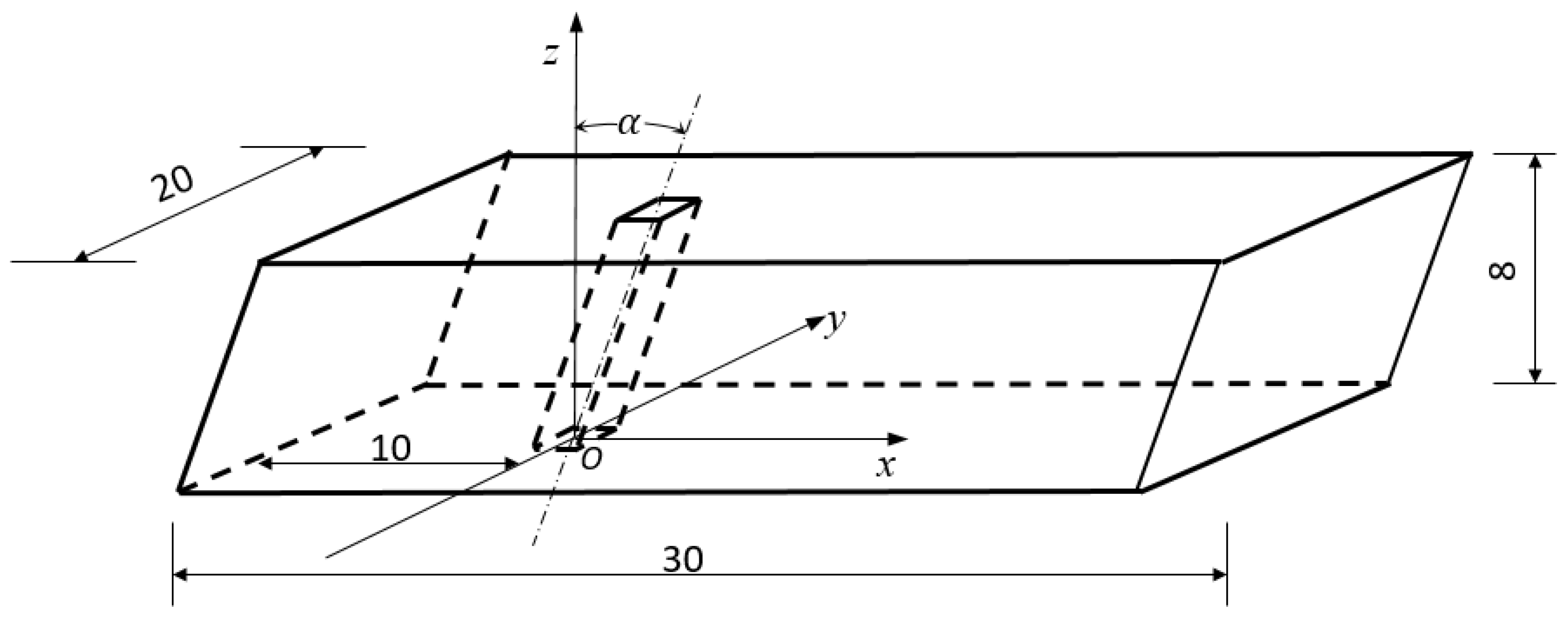
2. Materials and Methods

2.1. Numerical Method

In the current study, both the 3D Navier–Stokes (NS) equations and the continuity equation serve as the governing equations, which are

$$\frac{\partial u_i}{\partial t}+u_j\frac{\partial u_i}{\partial x_j}+\frac{\partial p}{\partial x_i}-\frac{1}{Re}\frac{{\partial }^2{u}_i}{\partial x_j^2}=0,$$

(1)

$$\frac{\partial u_j}{\partial x_j}=0,$$

(2)

where i and j represent 1, 2, and 3, with x₁, x₂, and x₃ referring to the Cartesian coordinates x, y, and z, which are defined such that the x-axis is the inlet flow direction, the y-axis is perpendicular to the inlet flow direction and the cylinder, and the z-axis is perpendicular to both x- and y-axes; u_i is the velocity component in the x_i direction, representing the velocity components u, $v$, and w, in the x, y, and z-directions, respectively; t is time; and p is pressure. The simulations are conducted in OpenFOAM (Version 2.2.0) C++ libraries, an open-source computational fluid dynamics package. The finite volume method (FVM) is adopted, and the governing equations are solved by the PISO (pressure implicit with splitting of operators) algorithm. Gauss cubic scheme (fourth-order) is used to discretize the convection term, whereas Gauss linear scheme (second-order) is used to discretize the diffusion term. The blended scheme (a second-order Crank–Nicolson scheme and a first-order Euler implicit scheme) is adopted for temporal discretization.

Figure 1 shows the rectangular computational domain with 30D × 20D × 8D in the x, y, and z directions, respectively, where D is the side length of the cylinder. According to Zhao et al. [10], the computational domain size in the z-direction should be at least 4D in order to obtain accurate predictions on the hydrodynamic forces of the cylinder. In consideration of the computational cost, the spanwise domain length for the present study is chosen as 8D. The cylinder length varies with the yaw angle α as 8D/cosα. In the streamwise direction, the inlet is set at 10D upstream of the cylinder while the outlet is set at 20D downstream of the cylinder. For the lower and upper boundaries, the free-slip boundary condition is not applicable, as discussed by Zhao et al. [10]. This is because the velocity in the spanwise direction is significant for a yawed cylinder while the free-slip boundary condition prohibits the flow from going through the boundaries. The boundary condition imposed on the lower and upper boundaries is described as follows:

u_i(x, y, z = 0, t) = u_i(x + 8Dtanα, y, z, = 8D, t),

(3)

p(x, y, z = 0, t) = p(x + 8Dtanα, y, z, = 8D, t).

(4)

This is to consider that both the computational domain and the grid lines (shown in the following section) are skewed at the yaw angle. The initial velocity and pressure within the whole domain are set to zero before a unit velocity U in the x-direction is applied at the inlet boundary. In the meantime, the outlet boundary has zero normal velocity gradient and zero pressure. A symmetric boundary condition with zero velocity component and zero pressure gradient is employed on the left and right boundaries that are parallel with the (x, z) plane. The no-slip boundary condition is then applied on the cylinder surface. The computations were performed in Pawsey Supercomputing Center, Western Australia. A total of 360 processors were used for each angle and the simulations were carried out up to a non-dimensional time of Ut/D = 1200 for all yaw angles, at which the fully developed equilibrium state vortex shedding was reached for enough time to allow the statistics to be calculated reliably.

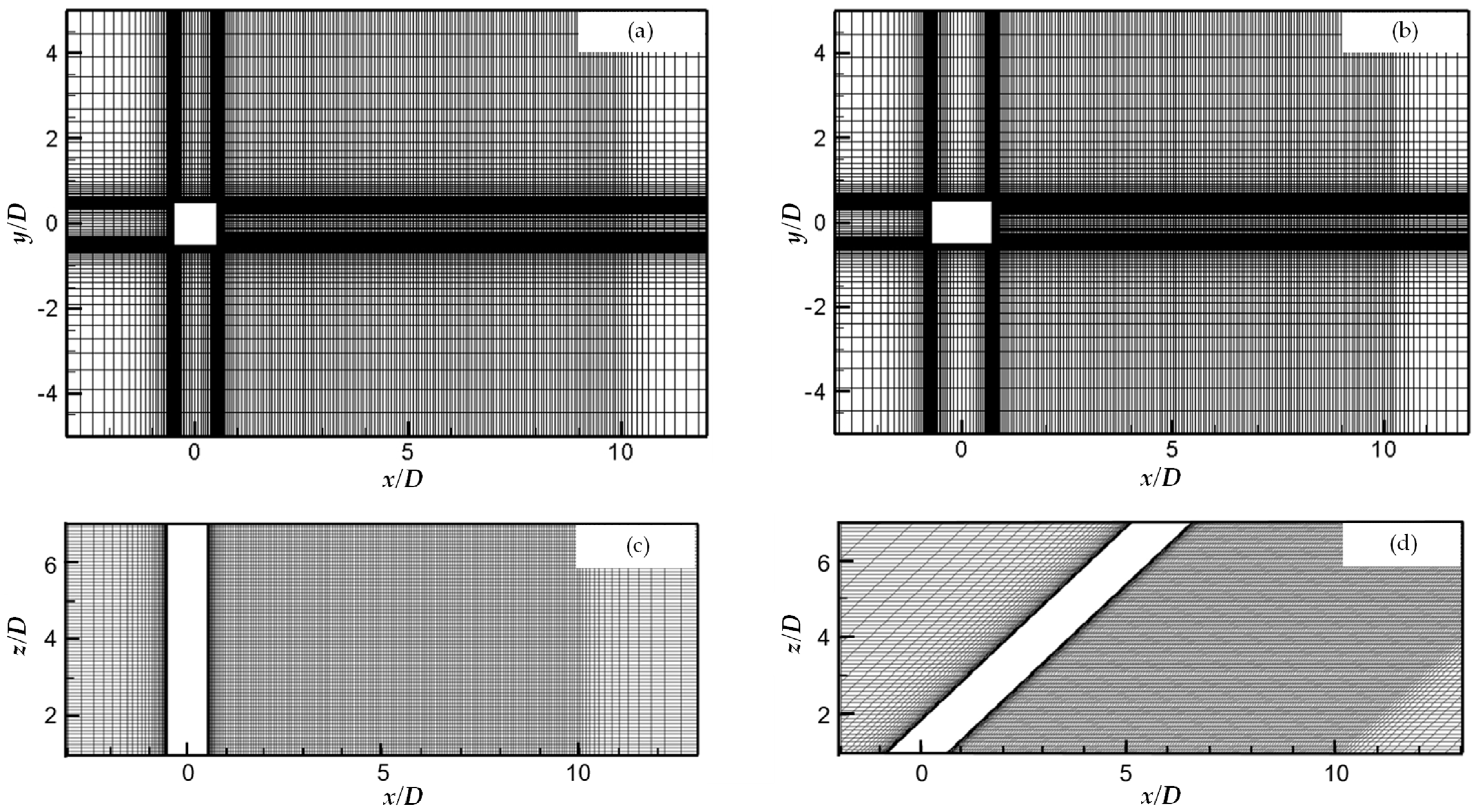
2.2. Mesh Dependence Check

On the (x, y) plane, a 2D mesh is first generated with a high resolution close to the cylinder and even higher resolutions at the tips of the cylinder. Up to x = 10D, a high-resolution mesh is also applied downstream of the cylinder in order to resolve the velocity and vorticity reliably. A close-up view of the reference mesh around the cylinder wall is shown in Figure 2a. The 2D mesh is then extended in the z-direction with certain layers to obtain the 3D mesh. A side view of the reference mesh is demonstrated in Figure 2c. As for the case of a yawed cylinder, the 2D mesh is extended obliquely along the cylinder axis to obtain the 3D mesh. The top view and side view of the meshes for α = 45° are also included in Figure 2 for reference. The mesh for α = 0° is employed for the mesh dependence check. The node number along the cylinder spanwise direction is 80, and that along the cylinder circumstance is 136, resulting in a mesh size of 0.1D in the spanwise direction and of 0.00734D next to the cylinder surface, respectively. In the streamwise direction, the size of the mesh is increased by a factor of 1.1 for the whole upstream as well as for downstream locations until x = 1D. For the region from x = 1D to 10D, the mesh size is maintained constant with that at x = 1D to generate meshes with a higher resolution. From x = 10D until the outlet boundary, the mesh size is continually increased by a factor of 1.1. In the transverse direction, the size of the mesh is increased by a factor of 1.1 until the left and right boundaries, respectively.

In the cylinder wall region, the simulation is very sensitive to mesh resolution. The mesh density around the cylinder wall can be evaluated by the non-dimensional distance between the first nodal point and the wall, which is normally defined as y⁺ = u_f∆/ν, where u_f is the maximum friction velocity and ∆ is the distance from the first layer of the mesh to the wall. The value of y⁺ is kept to less than 1 for all the cases in the present study in order to ensure that the boundary layer is captured with sufficient accuracy [24]. In the simulations for turbulent flows, the smallest resolved length scale is ideally required to be O(η) [25], where η (≡(ν³/ε)^1/4) is the Kolmogorov length scale and ε is the mean dissipation rate of the turbulent kinetic energy. Considering the fact that the main focus of the present study is on the large-scale vortex structures, the mean energy dissipation rate can be estimated approximately using ε ≈ $C_{\epsilon }$k^3/2/L [26,27], where k (≡½(u’² + v’² + w’²) is the turbulent kinetic energy (TKE), L is the integral length scale, and $C_{\epsilon }$ is a constant [28]. Hereafter, the superscript prime denotes the root-mean-square (rms) values. The TKE can be calculated by the velocity information obtained at each node in the flow field. For a given flow, with the increase of Taylor microscale Reynolds number Re_λ (≡u’λ/ν, where λ is the longitudinal Taylor microscale), the magnitude of η decreases, and as a result, the mesh size needs to be decreased correspondingly in order to keep the appropriate resolution for the simulations. However, it is worthwhile to point out that the requirement of grid sizes equal to or smaller than η may be too stringent, given that the Kolmogorov length scale is at the far end of the dissipative range, as previously discussed by Moin and Mahesh [29] and Trias et al. [25]. Vreman and Kuerten [30] showed that most of the dissipation in a turbulent channel flow occurs at scales greater than 30η. Zhang et al. [31] showed that a mesh size of 3.5η is sufficed to obtain reliable results for a turbulent square duct flow using DNS, which seems in agreement with the suggestion by Wallace and Foss [32], based on the evaluation of Antonia et al. [33] in a channel flow, that an optimal separation distance of 2η to 4η is adequate for velocity derivative measurements. It also agrees with that reported by Zhou et al. [34] in the near wake of a circular cylinder at Re = 2500. For the present simulation, the value of ε peaks at the shear layer regions, resulting in the smallest values of η around these regions. The magnitudes of ∆x/η and ∆y/η are very comparable to those reported by Trias et al. [25], where the maximum values of about 6 and 3.5 for ∆x/η and ∆y/η, respectively, are obtained at x ≤ 1.5D. With further increase of the downstream location, the magnitude of ε decreases (and hence η increases), whereas both ∆x and ∆y increase. As a result, the values of ∆x/η and ∆y/η till x = 10D are still comparable with those at x ≤ 1.5D. Therefore, the length scales of the mesh applied in the present simulations are fine enough to resolve the turbulent flow structures.

The time step ∆t is chosen based on the criterion that the Courant number Co (= $\left|u\right|$∆t/∆l) should be kept below 0.5 for the entire domain, where $\left|u\right|$ is the magnitude of the velocity through a cell and ∆l is the cell size in the direction of the velocity. In this case, the non-dimensional time step is calculated as U∆t/D = 1.5 × 10⁻³. A finer mesh, with even higher resolution around the cylinder, is also generated for the mesh dependence check.

Table 1. Main parameters of the coarse and fine meshes used in the present study.

Mesh Type	Coarse	Fine	Coarse (Refined in z-Direction)
Node number along cylinder circumstance	136	200	136
Node number along cylinder spanwise length	80	80	160
Mesh size next to the cylinder surface	0.00734D	0.00503D	0.00734D
Total node number	2,376,640	3,608,160	4,753,280

lists the mesh characteristics of both the coarse (reference) mesh and the fine mesh. In addition to the mesh dependence check, a refined mesh by doubling the number of layers of the coarse mesh in the z-direction is employed as well, to examine the mesh sensitivity in the spanwise direction, and the mesh details are also included in Table 1.

The mesh dependence is evaluated in terms of the drag coefficient $C_D$, lift coefficient $C_L$, Strouhal number St, and the base pressure coefficient $C_{pb}$, which are defined as:

$$C_D=F_D/(½\rho U^{2}DL),$$

(5)

$$C_L=F_L/(½\rho U^{2}DL),$$

(6)

$$St=f_{s}D/U,$$

(7)

$$C_{pb}=(p_b-p_{\infty })/(½\rho U^2),$$

(8)

where $F_D$ is the total drag on the cylinder, $F_L$ is the total lift, St is the Strouhal number, $f_s$ is the vortex shedding frequency, p_b is the time-averaged base pressure measured at the rear stagnation point of the cylinder, p_∞ is the reference pressure at the inlet boundary, and ρ is the density of the fluid. The simulation results of the Strouhal number St, the time-averaged and rms values of the drag coefficient ${\overline{C}}_D$ and $C_D^{\prime }$, the rms value of the lift coefficient $C_L^{\prime }$, and the time-averaged base pressure ${\overline{C}}_{pb}$ obtained from the three types of mesh, together with results from previous studies, are listed in

Table 2. Mesh dependence check for a square cylinder in crossflow (α = 0°). The relative errors in the brackets are calculated by using the results obtained from the coarse mesh as reference values.

Case	St	${\overline{\mathit{C}}}_{\mathit{D}}$	${\mathit{C}}_{\mathit{D}}^{\prime }$	${\mathit{C}}_{\mathit{L}}^{\prime }$	$-{\overline{\mathit{C}}}_{\mathit{p}\mathit{b}}$
Present DNS study, coarse mesh	0.124	2.11	0.186	1.49	1.42
Present DNS study, fine mesh	0.121 (2.4%)	2.13 (1.0%)	0.194 (4.3%)	1.47 (1.3%)	1.45 (2.1%)
Present DNS study, coarse mesh refined in z-direction	0.125 (0.8%)	2.10 (0.5%)	0.188 (1.0%)	1.45 (2.7%)	1.40 (1.5%)
Saha et al. [17], DNS study, Re = 500	0.120	2.14	0.193	1.442	-
Sohankar [21], LES study, Re = 1000	0.119	2.08	0.210	1.43	-
Hwang and Sue [37], numerical study, Re = 1100	0.123	2.052	0.036	1.271	-
Norberg [35], wind tunnel experiment, Re = 5000	0.129	2.21	-	-	1.45
Kumar et al. [36], water channel experiment, Re = 5200	0.123	1.95	-	1.50	1.11

. First of all, it is noticed that the differences in St, ${\overline{C}}_D$, $C_D^{\prime }$, $C_L^{\prime }$, and ${\overline{C}}_{pb}$ between the coarse mesh and the fine mesh are about 2.4%, 1.0%, 4.3%, 1.3%, and 2.1%, respectively, which indicate the negligible effect of the mesh density, and thus the coarse mesh is sufficient for the prediction of the vortex shedding frequency and hydrodynamic forces. Secondly, the results obtained from the coarse mesh refined in the z-direction are found to be very close to those obtained from the coarse mesh according to the relative errors calculated by using the results of the coarse mesh as reference values. The coarse mesh should provide precise simulations in the current study. Thirdly, the results of the present simulations are consistent with those of previous experimental [35,36] and numerical [17,21,37] studies for a square cylinder in crossflow. It should be noticed that the significantly small value of $C_D^{\prime }$ and the relatively small value of $C_L^{\prime }$ from the study by Hwang and Sue [37] are attributed to the effect of aspect ratio as their simulations are based on a 2D model. As for the smaller absolute value of $-{\overline{C}}_{pb}$ from the study by Kumar et al. [36], the difference should result from the larger formation length of the recirculation region at a larger Reynolds number. In general, the present simulations provide satisfactory results with regard to the vortex shedding frequency and the force characteristics. To save the calculation time, the coarse mesh is applied in the present study for all yaw angles. In addition, the profiles of the time-averaged streamwise and transverse velocities at different downstream locations (x = 1D, 2D, 5D, and 10D) calculated with the coarse mesh are demonstrated in Figure 3 and Figure 4, respectively. Available results at similar downstream locations from previous experimental [15,19,38] and numerical [18,39] studies are included in the figures as well for comparison. Based on the figures, it can be concluded that the results are in good agreement with the published ones, validating the present setup for the simulations.

3. Results

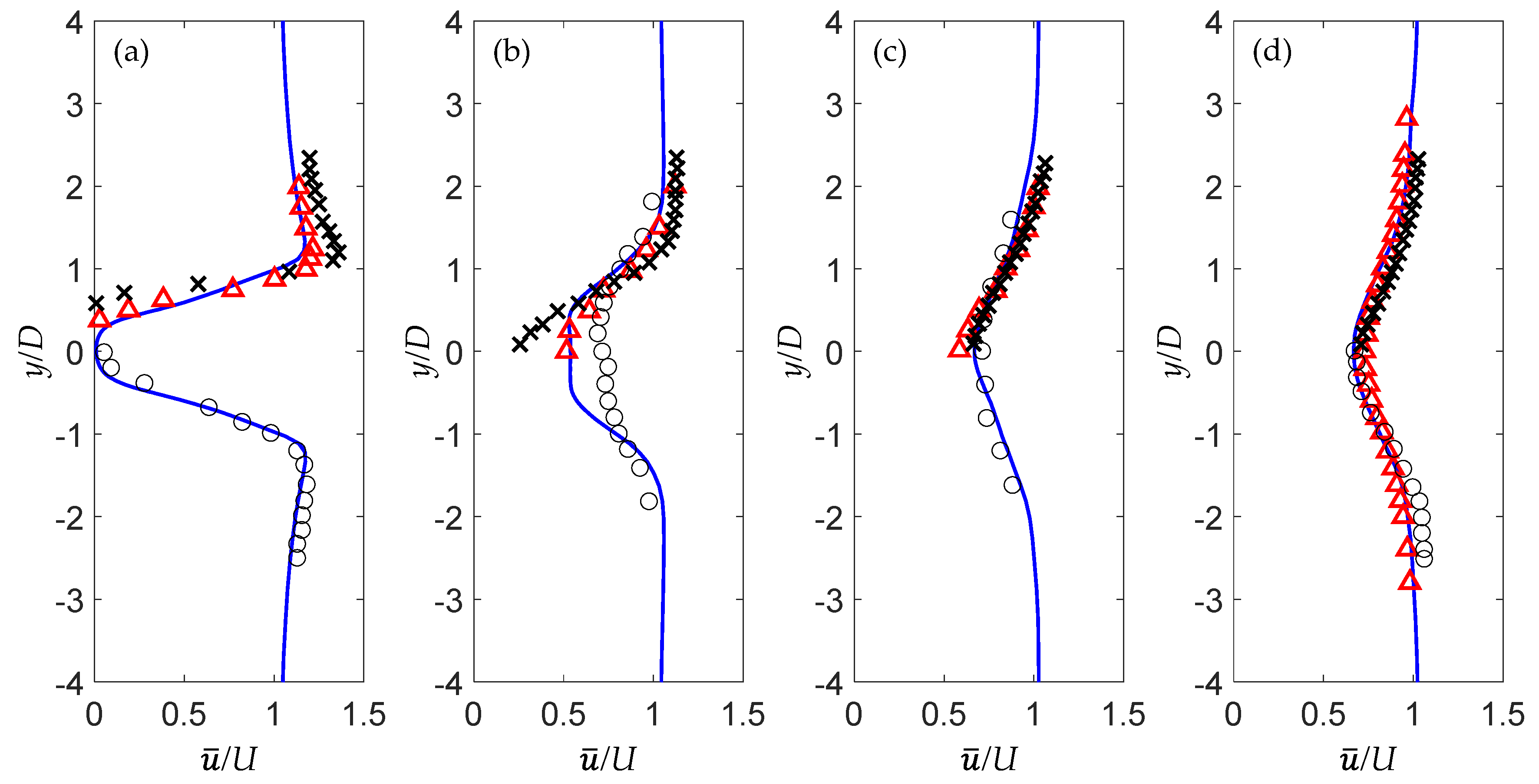
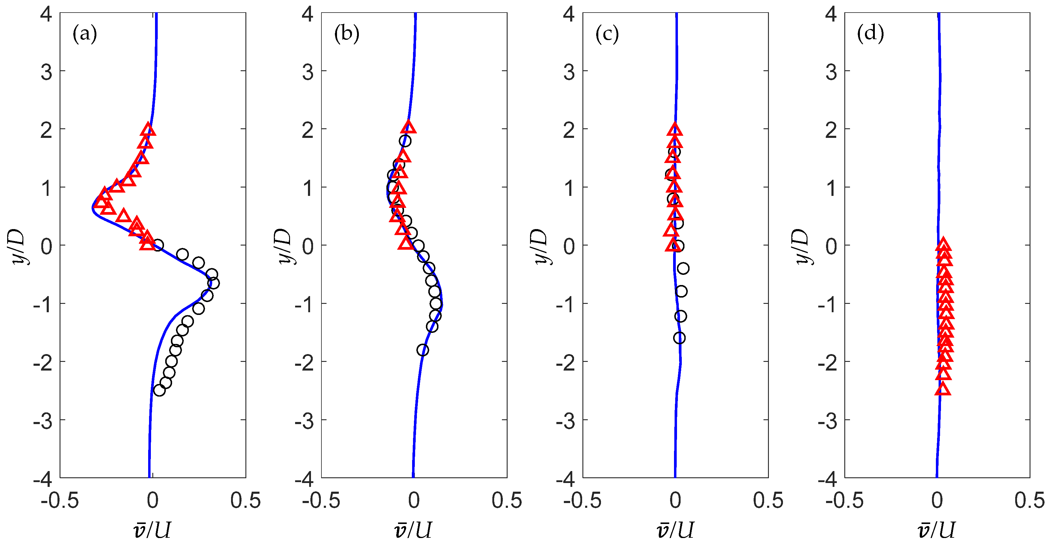
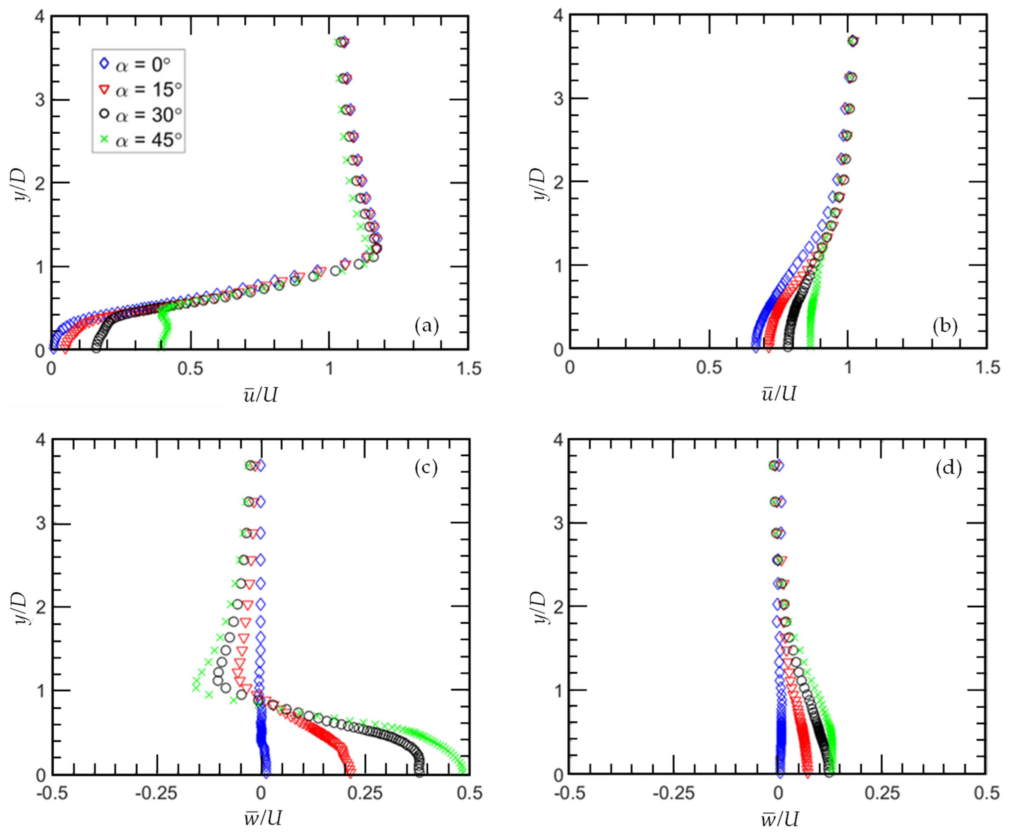
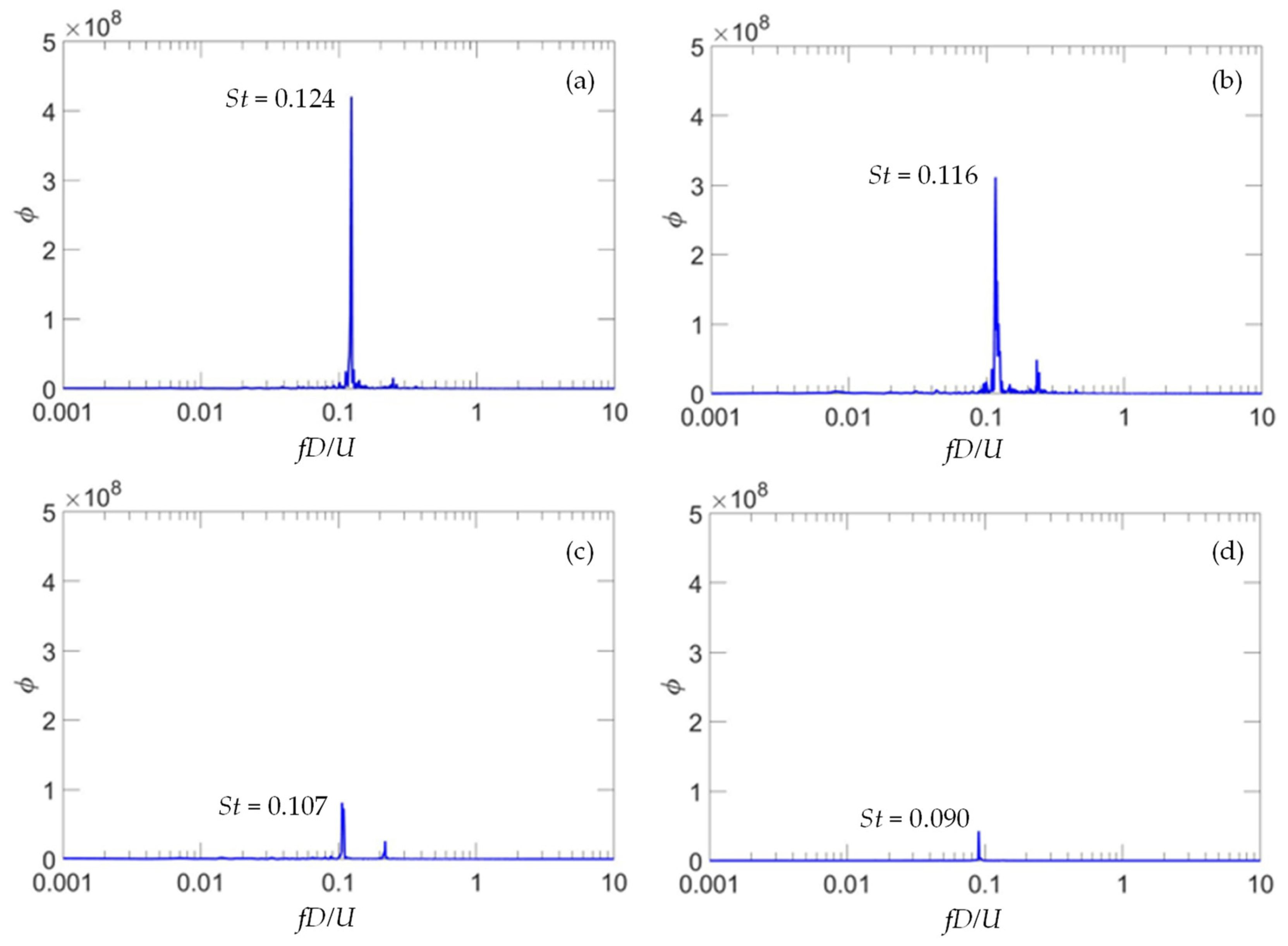
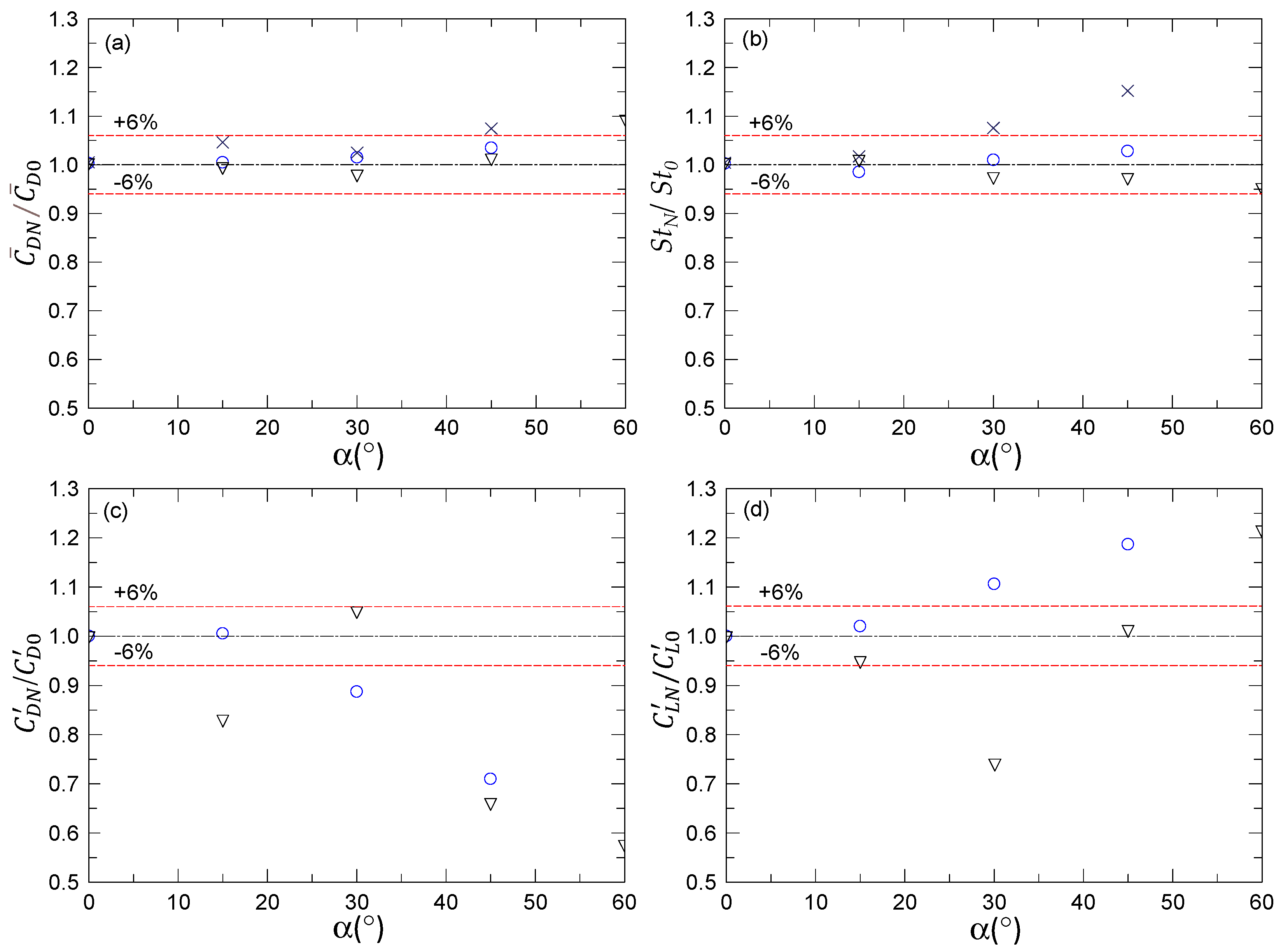
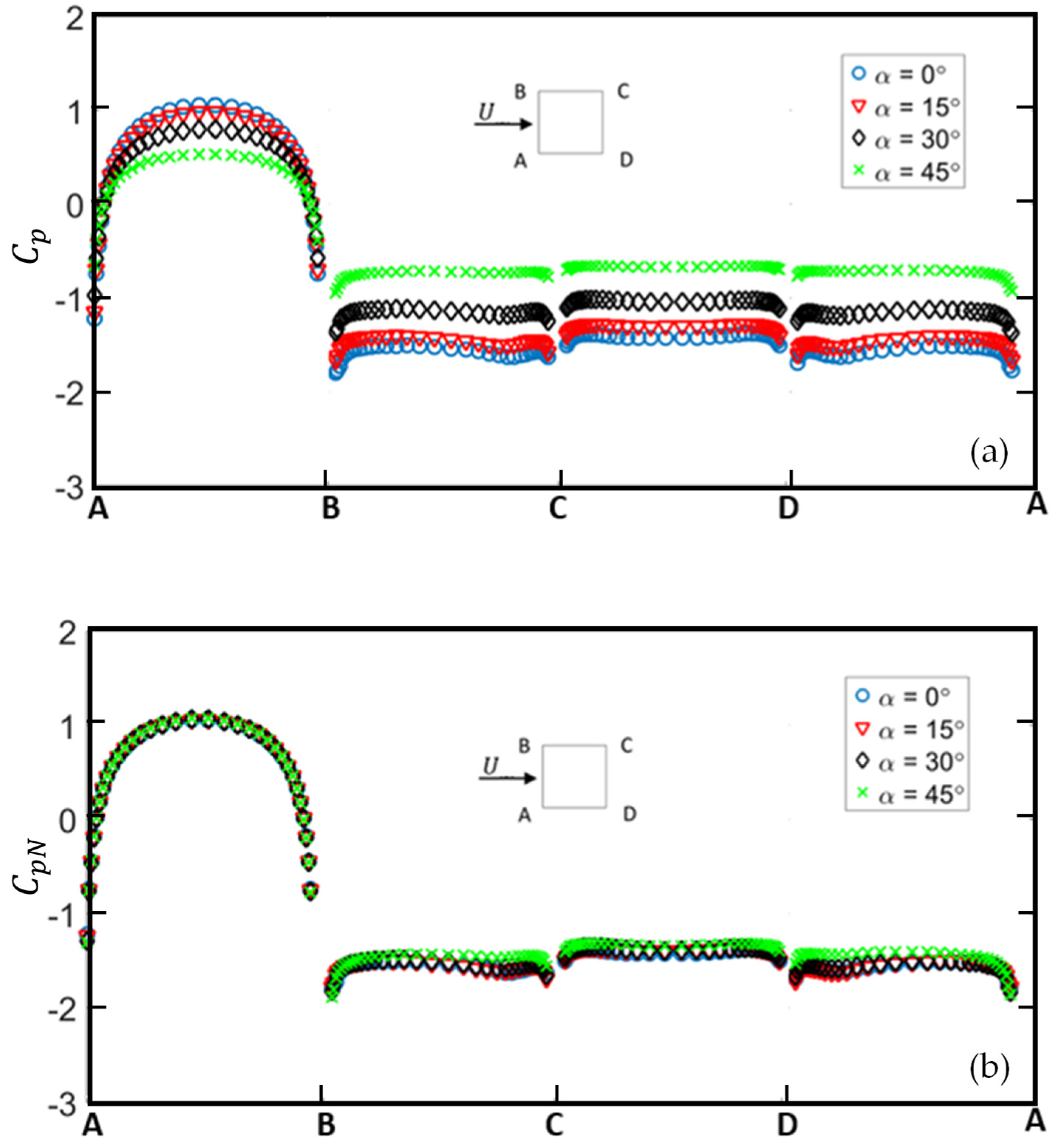
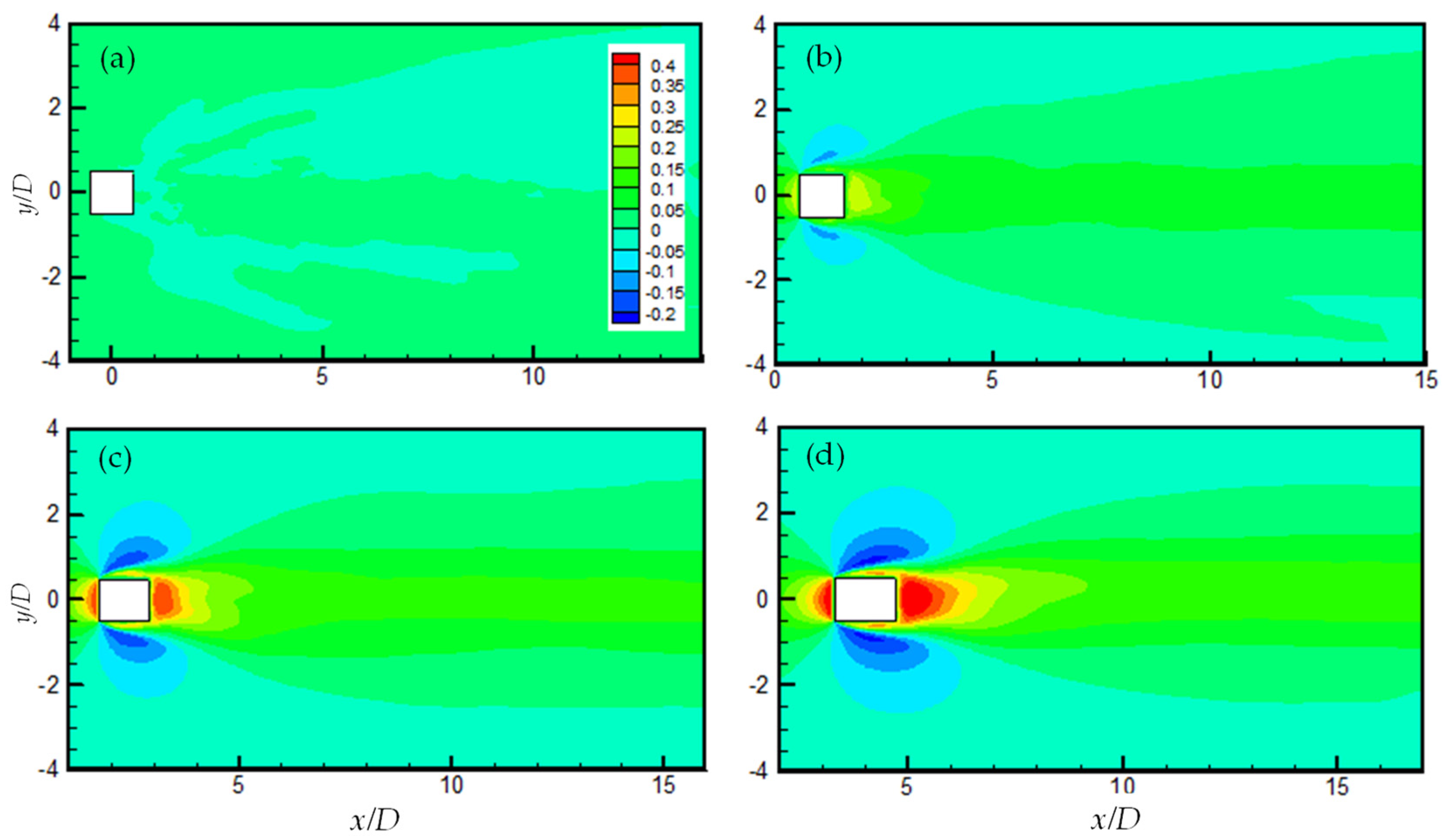
3.1. Velocity Profile, Force Coefficients, and Vortex Shedding Frequency

Profiles of the streamwise mean velocity $\overline{u}$/U at two different downstream locations (x = 1D and 10D) for all yaw angles are shown in Figure 5a,b. The profiles are averaged over the whole calculation time and the cylinder span. Only half of the profile is shown here due to its symmetric distribution about the wake centerline (y/D = 0) where the largest velocity deficit appears. At x = 1D, the maximum value of $\overline{u}$/U for α = 0° is about 17% higher than the unity freestream velocity due to blockage effects and it appears at y/D = 1.3, which is in agreement with that obtained by Lyn et al. [15]. As α increases, the maximum value of $\overline{u}$/U shows a decreasing trend and the position of the maximum value shifts slightly towards the centerline. It can be seen that the velocity deficit decreases significantly with the increase of α due to the gradually disappeared recirculation region. In addition, the profile of $\overline{u}$ at α = 45° displays a smaller wake width than that of α = 0° and this will lead to a faster recovery of the streamwise velocity for α = 45°, as the ambient flow feeds faster into a narrower wake than into a wider one. Additionally, a narrower wake at large yaw angle leads to a higher base pressure and a smaller drag coefficient, which is shown in the subsequent section. At x = 10D, the velocity deficit remains a decreasing trend with the increase of α, and this denotes the weakening vortex shedding process at large yaw angles since the smaller velocity deficit reflects the weaker separating process of shear layers.

Figure 5c,d demonstrate the profiles of the spanwise mean velocity $\overline{w}$/U at x = 1D and 10D for all yaw angles. The distributions of $\overline{w}$/U at both locations remain symmetric about y/D = 0, although their magnitudes are much smaller than those of $\overline{u}$/U. The spanwise velocity is a measure of the three-dimensionality of the flow. A larger magnitude of $\overline{w}$/U should imply a higher level of three-dimensionality. At x = 1D, $\overline{w}$/U is close to zero for α = 0°, as expected for a quasi-two-dimensional wake. The magnitudes of $\overline{w}$/U on the centerline increase significantly from 0.01 to 0.48 as α varies from 0° to 45°, respectively, indicating an increasingly stronger secondary flow along the cylinder axis. This secondary flow decreases away from the centerline, and at around y/D = 0.9, the secondary flow changes its direction, with a maximum spanwise velocity occurring at y/D = 1.2. At x = 10D (Figure 5d), the distributions of $\overline{w}$/U across the wake still experience an increasing trend with the increase of the yaw angle, in agreement with the previous study by Lou et al. [19]. For α = 0°, the nearly zero value of $\overline{w}$/U is in agreement with the quasi-two-dimensional wake. When α increases, the enhanced spanwise velocity acts to impair the two-dimensionality of the wake and reduces the strength of the vorticity. The strong spanwise velocity at the near wake can make the interaction of the shear layers difficult, thus weakening the vortex shedding process, especially for α = 45°.

The force coefficients for different yaw angles are calculated when the equilibrium state of the simulations is reached for a sufficiently long time. The results of the mean drag coefficient and the rms values of the drag and lift coefficients for different yaw angles are listed in

Table 3. Force coefficients and Strouhal numbers for different yaw angles.

α	${\overline{\mathit{C}}}_{\mathit{D}}$	${\mathit{C}}_{\mathit{D}}^{\prime }$	${\mathit{C}}_{\mathit{L}}^{\prime }$	St	${\overline{\mathit{C}}}_{\mathit{D}\mathit{N}}$	${\mathit{C}}_{\mathit{D}\mathit{N}}^{\prime }$	${\mathit{C}}_{\mathit{L}\mathit{N}}^{\prime }$	StN
0°	2.110	0.186	1.490	0.124	2.110	0.186	1.490	0.124
15°	1.969	0.174	1.418	0.116	2.110	0.187	1.520	0.120
30°	1.596	0.124	1.236	0.107	2.128	0.165	1.648	0.124
45°	1.086	0.066	0.884	0.090	2.172	0.132	1.768	0.127

. It can be seen that all the force coefficients decrease with the increase of α. The significant decrease with the increase of α can be attributed to the narrower wake and less vigorous vortex shedding at larger yaw angles as mentioned previously. This result also indicates that energy is transferred from the spanwise vorticity to the streamwise vorticity, which is discussed in the subsequent section.

The spectra of the lift force for different yaw angles are calculated and the results are shown in Figure 6. The spectrum is obtained by calculating FFT (fast Fourier transform) of the time series of the lift coefficient. The dominant frequency, corresponding to the peak on the spectrum, represents the vortex shedding frequency f_s, or the Strouhal number St. The results of St for different yaw angles are also included in Table 3. In Figure 6, the spectra for α = 0°, 15°, and 30° all display pronounced peaks which reflect the strong vortex shedding process. Although the peak on the spectrum is still discernible at α = 45°, the energy of the peak shows a dramatic decrease, which reflects the significant reduction in the vortex shedding intensity. The decrease ratio of 90% in the peak energy on the spectrum as α varies from 0° to 45° is higher than that of the yawed circular cylinder [6] and, hence, the effect of the yaw angle on vortex shedding is stronger for a square cylinder than that for a circular one. The Strouhal number demonstrates a decrease trend from St = 0.124 at α = 0° to St = 0.116, 0.107, and 0.090 at α = 15°, 30°, and 45°, respectively.

To verify the validity of the IP, the velocity component normal to the cylinder axis U_N (≡Ucos(α)) is used in the calculation of the force coefficients and the Strouhal number, denoted as ${\overline{C}}_{DN}$, $C_{DN}^{\prime }$, $C_{LN}^{\prime }$, and St_N, where the subscript N denotes normalizations by the velocity component U_N. These values are listed in Table 3. The mean drag coefficients ${\overline{C}}_{DN}$ are found to be 2.110, 2.128, and 2.172 for α = 15°, 30°, and 45°, respectively. Compared with that at α = 0°, the deviation in ${\overline{C}}_{DN}$ is about 3% for α = 45° and even smaller for the other angles. Similarly, the Strouhal number St_N (≡f_sD/U_N) for α = 15°, 30°, and 45° is found to be 0.120, 0.124, and 0.127, respectively. The deviation in St_N at α = 45° from that at α = 0° is only about 2.5%, which should support the validity of the IP even at 45° for a square cylinder. The above results indicate the validity of the IP for predicting the first-order statistics of the drag coefficient and Strouhal number when the yaw angle reaches 45°, in agreement with the results reported by Zhao et al. [14]. As for the rms values of the force coefficients, $C_{DN}^{\prime }$ decreases whereas $C_{LN}^{\prime }$ increases with the increase of α. These trends are consistent with those shown by Zhao et al. [10]. Compared with the results at α = 0°, it seems that both $C_{DN}^{\prime }$ and $C_{LN}^{\prime }$ at yaw angles α > 25° based on the trends in the figures) depart apparently from IP, indicating that IP fails in predicting the second-order force statistics, supporting the results by Zhao et al. [14] for yawed circular cylinder wakes.

If the force coefficients and the Strouhal number at different yaw angles are normalized by their counterparts at α = 0° (denoted by a subscript zero), the ratios should equal 1 if IP is valid. The results of the above ratios at different yaw angles are demonstrated in Figure 7, together with those from the previous experimental studies on a yawed square cylinder [19], as well as the numerical results for a yawed circular cylinder [10]. It can be seen that the numerical results of ${\overline{C}}_{DN}/{\overline{C}}_{D0}$ (Figure 7a) and St/St₀ (Figure 7b) obtained by both the present study and that of Zhao et al. [10] satisfy the IP favorably over the angles examined. Even if a tolerance of 6% is allowed for the experimental uncertainty, the numerical results still indicate a larger yaw angle range over which the IP is valid for a square cylinder compared with the experimental results [19]. These results are apparently different from the experiments [19]. The departure of the second-order force coefficients $C_{DN}^{\prime }$/$C_{D0}^{\prime }$ (Figure 7c) and $C_{LN}^{\prime }/C_{L0}^{\prime }$ (Figure 7d) from 1 indicate that IP is not valid for these cases, at least for α ≥ 25°.

The distributions of the pressure coefficient around the cylinder surface are also examined. The pressure coefficient is defined as $C_p$ = (p − p_∞)/(½ρU²), where p is the time-averaged pressure measured on the cylinder surfaces, and the results for α = 0° are demonstrated in Figure 8, together with results from the previous experimental [35] and numerical studies [16]. The flow approaches the cylinder from left to right; hence, side AB is the leading edge and side CD is the trailing edge. As shown in Figure 8, the pressure coefficients are symmetric about the wake centerline on both the leading edge and the trailing edge. The distribution displays a parabolic shape on the leading edge and attains the highest magnitude of unity at the stagnation point, which agrees well with the published results shown in the figure and validates the present simulations. Some differences in $C_p$ from the previous studies can be observed at the trailing edge, as well as at the top (BC) and bottom (AD) edges, which should be attributed to the differences in Reynolds numbers. For the yawed square cylinder, the results of $C_p$ for all angles investigated in the present study are shown in Figure 9a. It can be seen that $C_p$ on the leading edge decreases with the increase of the yaw angle, from which a difference of about 50% in $C_p$ can be found between α = 0° and 45°. However, $C_p$ on the other three edges increases when α varies from 0° to 45°. Therefore, the pressure difference between the leading and trailing edges decreases as α increases, which results in smaller mean drag coefficients for larger yaw angles. This result is similar to the finding for a yawed circular cylinder [10]. However, when U_N is used to normalize the pressure coefficient, i.e., $C_{pN}$ = (p − p_∞)/(½ρ$U_N^2$), there is practically no difference in $C_{pN}$ on the leading edge for all yaw angles, as demonstrated in Figure 9b. For α = 0°, 15°, and 30°, the differences in $C_{pN}$ on the trailing edge, as well as on the top and bottom edges, are also negligible. As a result, the pressure coefficient at the leading edge supports the IP well to 45° for a square cylinder. However, on the trailing edge, the value of $C_{pN}$ at α = 45° is 6% higher on average than that at α = 0°.

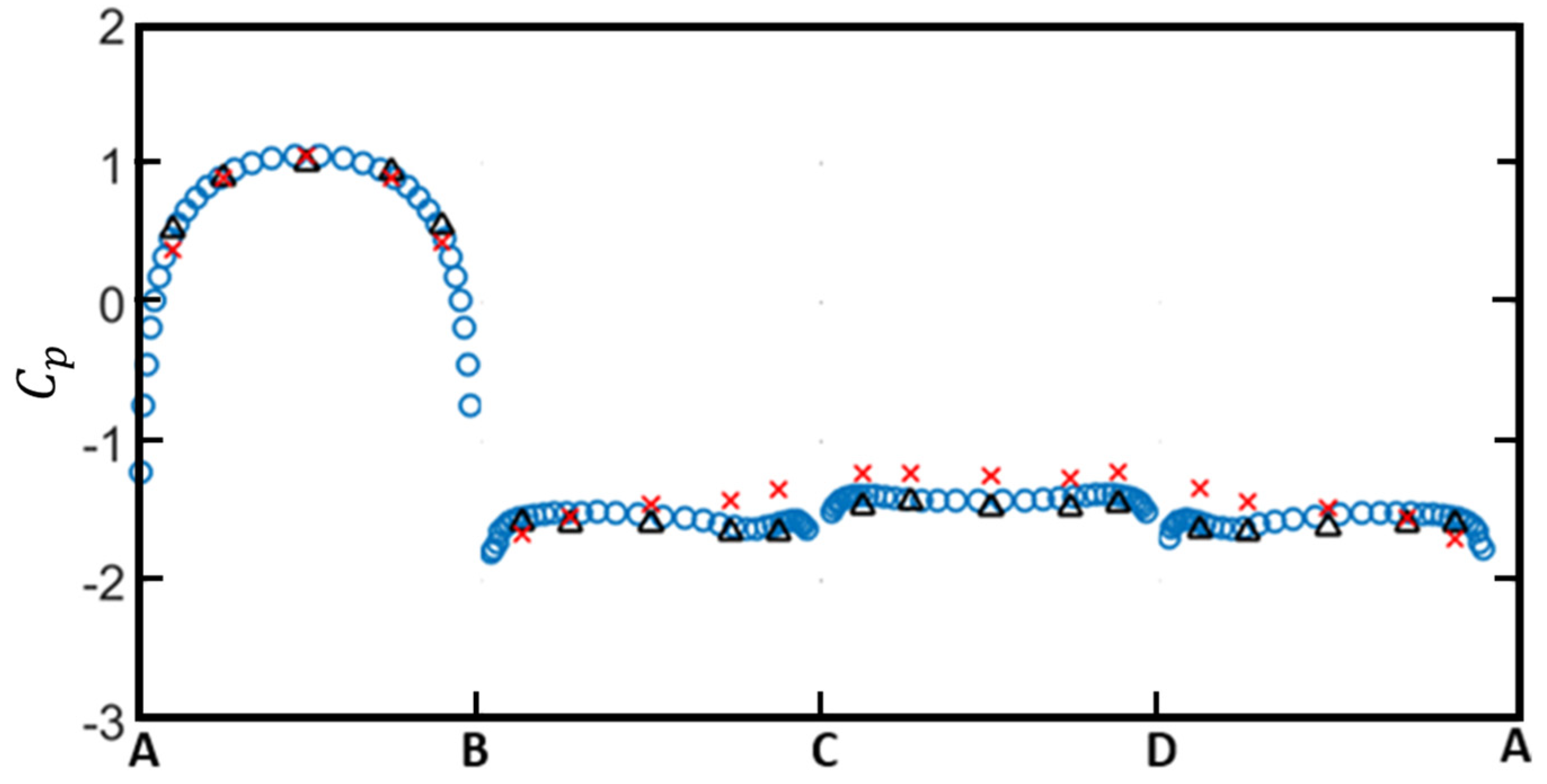
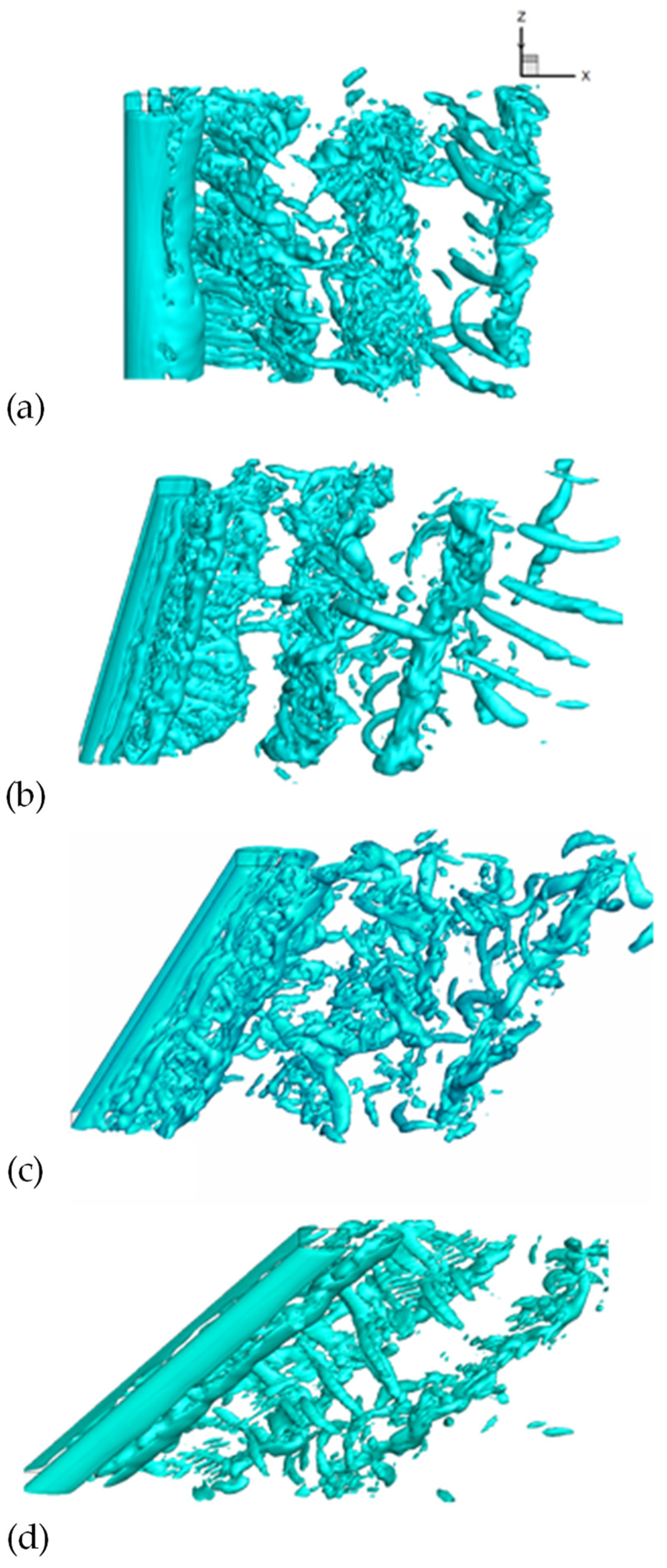
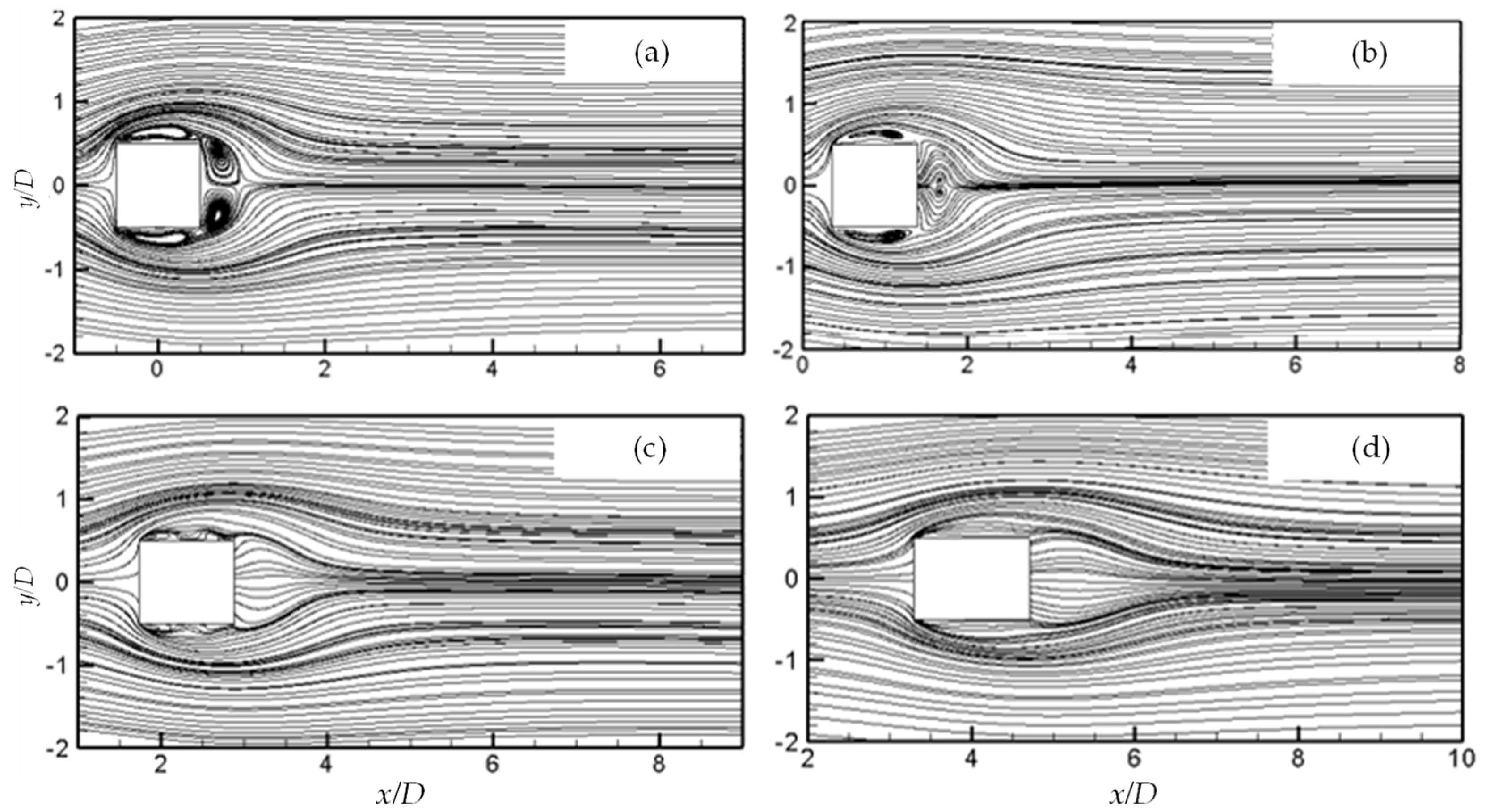
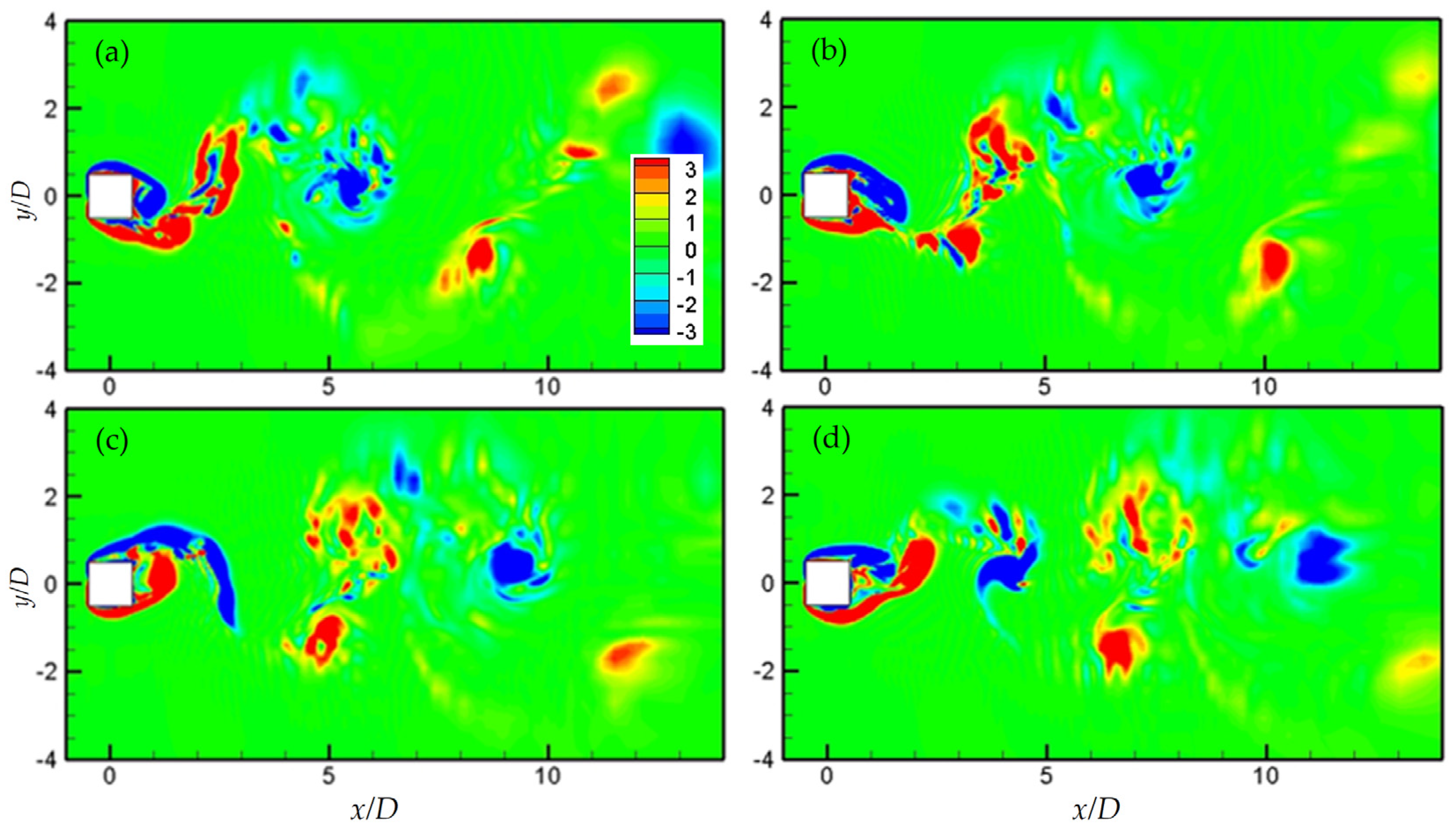
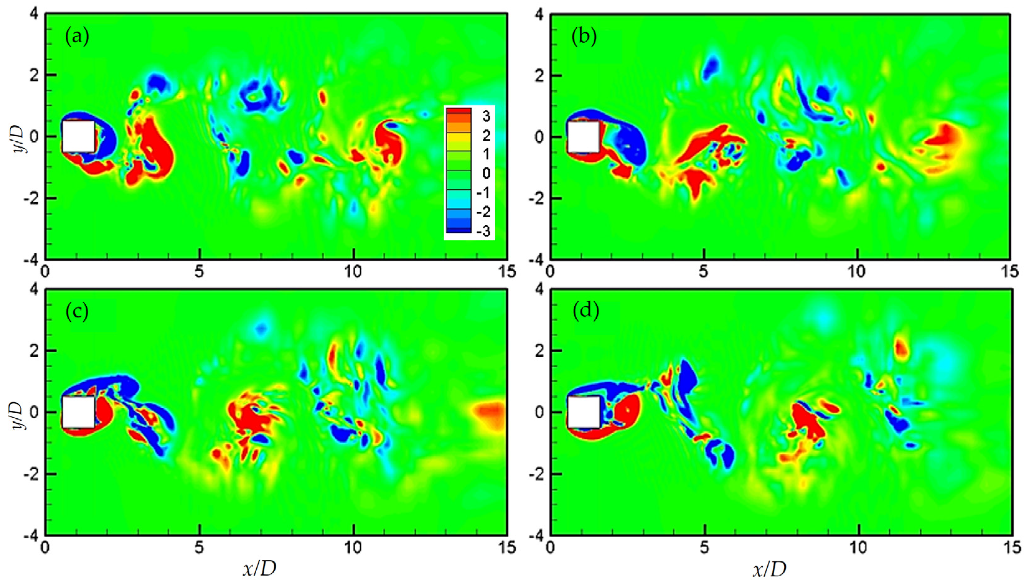
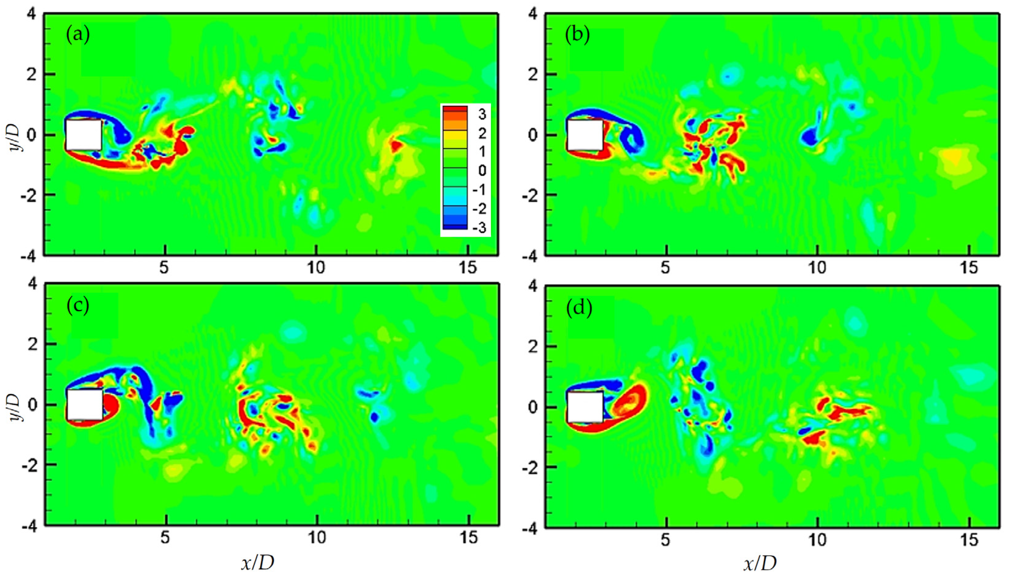
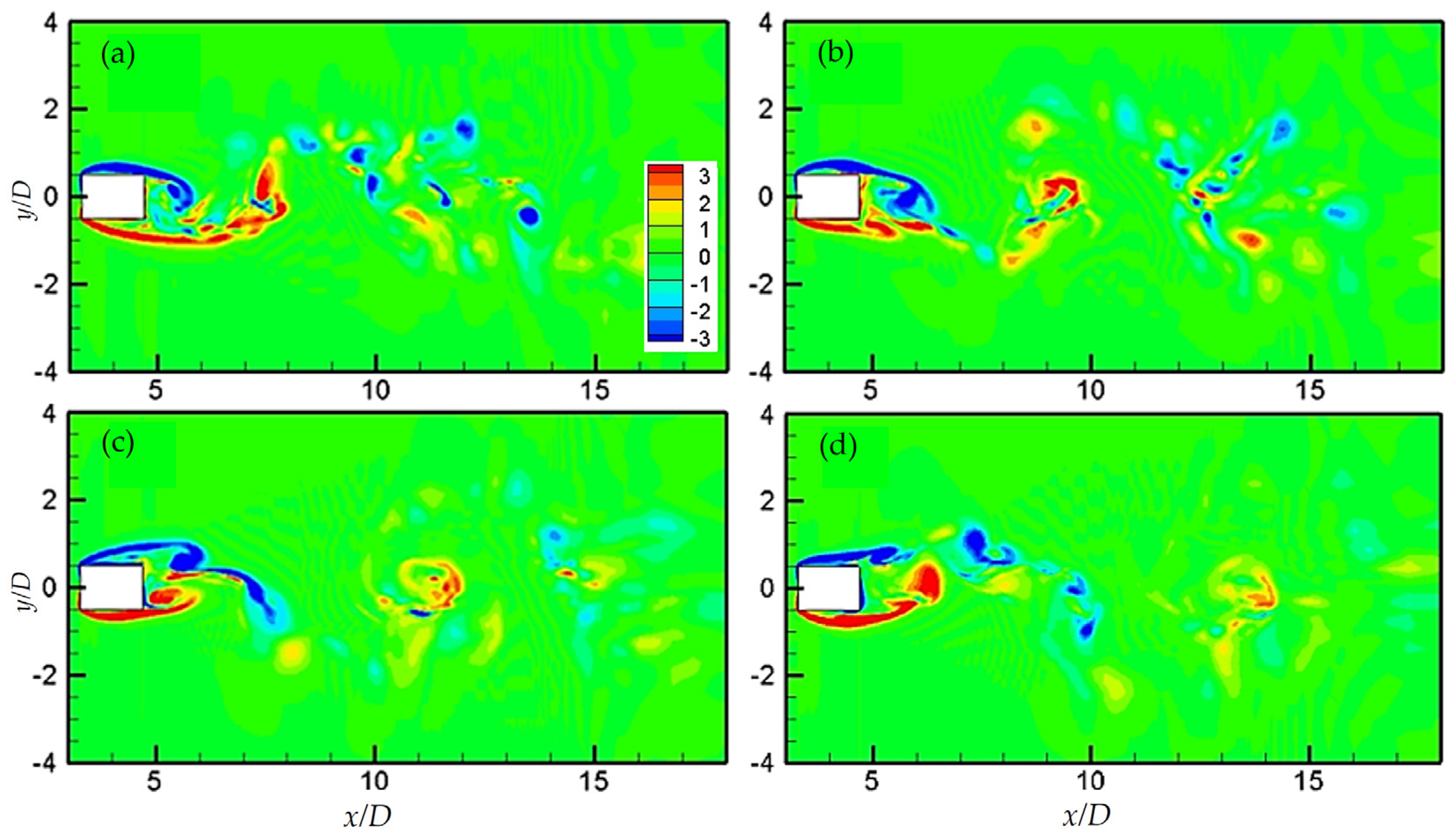
3.2. Flow Structures

First of all, the iso-surface of λ₂ is used as the identification of the vortex structures [40]. Figure 10 shows the instantaneous iso-surfaces of λ₂ = −1 at the same phase for different yaw angles till x = 10D (Figure 2). The flow is totally 3D, as one can see that the spanwise vorticity becomes wavy and the streamwise vorticity is also irregular with a large wavelength in the spanwise direction. Generally, the spanwise vorticity in λ₂ iso-surfaces still keeps the inclination that parallels with the cylinder axis. The vortex shedding process is not as organized as that in a circular cylinder wake at the same Reynolds number [10]. A structure named mode B, which is characterized by the counter-rotating vortex pairs in the direction perpendicular to the cylinder axis and reported to persist up to Re = 1000 by Zhao et al. [41] for the circular cylinder, can also be recognized in Figure 10. Compared with that of a circular cylinder wake [42], the pattern of mode B structure obtained from the present square cylinder is less organized. At α = 0°, the spanwise vorticity dominates the wake and generally shows organized shape of tubes along the streamwise direction. A tube is about to shed from the cylinder, but its shape is not uniform along the cylinder axial direction as the vortices are not shed at the same phase due to the 3D effect. Even though the spanwise vortices are generally parallel with the cylinder axis, they can align in other directions locally. The spanwise vortex tubes are still strong enough to be recognized at x = 10D. As α increases to 15°, the vortical structures become smaller and also the phase difference along the axial direction becomes more apparent. At α = 30° and 45°, fewer spanwise vorticity tubes are observed and the shape of the tubes becomes much less organized, and yet they are all parallel with the cylinder, i.e., keeping parallel shedding. In addition, some rib-like structures start to show up and they are either mixed with the spanwise vortices or connecting two spanwise tubes. At large yaw angles, the iso-contours seem to break up into small-scale structures rather fast. This is attributed to the enhancement of the streamwise vortices which wrap around the spanwise vortices and induce the instability of the primary spanwise vortices. The significant differences in the spanwise vortex shedding at α = 30° and 45° also indicate that the yaw angle affects the square cylinder wake more than that of the circular one, which was shown by Zhao et al. [10], where the spanwise vortices with low intensity and twisted shape are still found at α = 60°. For the streamwise vorticity, even though some rib-like structures can be observed, they are not well-formed. As α increases from 0° to 45°, the streamwise vorticity in λ₂ iso-surfaces becomes more and more discernible. At α = 45°, a row of rib-like vortices is generated right downstream of the cylinder and sheds perpendicularly to the cylinder axis, which is similar to that in the circular cylinder wake [10]. The strong streamwise vortices occupy the wake area as demonstrated in Figure 10d, with smaller spanwise wavelengths and more regular patterns.

For a better view of the shedding process of the spanwise vortices, the evolution of the spanwise vorticity ω_z contours viewed on the (x, y) plane is of interest to investigate. Prior to examining the spanwise vorticity on the (x, y) plane, the time-averaged streamlines at different yaw angles are firstly depicted in Figure 11. As the plane is extracted at z = 4D, the coordinate of the cylinder center varies with the yaw angle. At α = 0°, a pair of counter-rotating vortices show up right downstream of the cylinder in a symmetric form. The foci and saddle points can be clearly identified in the figure. The saddle point locates at approximately x = 1.1D (measured from the center of the square), which is the same as that found by Oudheusden et al. [43]. At the upper and lower edges of the cylinder, two recirculation regions can be observed, which also show that there is no reattachment to the cylinder wall for the flow separated from the leading edge. This recirculation region, however, is found to be absent in the wake of a circular cylinder. When α increases to 15°, although the recirculation regions on upper and lower edges still exist, the counter-rotating vortex pairs are hardly identified due to the generation of the spanwise velocity. This phenomenon, according to Najafi et al. [44], takes place at α = 25° for a circular cylinder. Similarly, at α = 30°, the enhanced spanwise velocity makes the counter-rotating region disappear completely, and the recirculation regions on the upper and lower edges show a reduction in size. Further, at α = 45°, the topology of the streamline becomes so simple that even the recirculation regions on the top and the bottom sides of the cylinder are absent entirely.

The evolutions of the ${\omega }_z$ contours viewed on the (x, y) plane for different yaw angles are shown in Figure 12, Figure 13, Figure 14 and Figure 15. For each angle, the instantaneous contours are demonstrated at four different phases with an increment of ¼T, where T is the vortex shedding period. One should be aware that the vortex shedding period varies for each angle, which corresponds to the Strouhal number listed in Table 3. In Figure 12, the primary vorticity contours are still discernible and keep well-organized shapes even at x = 10D for α = 0°. The length of the vortex formation region for α = 15° almost shows no change compared with that at α = 0°, according to Figure 13. However, the contours are not as organized in shape as those at α = 0°, and some small-scale structures start to appear. The ${\omega }_z$ contours at α = 30° in Figure 14 appear to be even less organized than those at α = 15°, and more small-scale structures can be observed. Beyond the vortex formation region, the strength of the vorticity decreases rapidly in the streamwise direction. When α increases to 45° (Figure 15), the upper and lower shear layers become more stretched in the streamwise direction than those at smaller yaw angles. The shear layers show no reattachment on either the top or the bottom surfaces and they do not interact with each other immediately downstream of the cylinder to form the Kármán-type vortices. This should be because of the axial flow generated near the base of the yawed cylinder, which makes the communication between the shear layers more difficult. Compared with the results at other angles, the wake width appears to be the smallest for α = 45°, which corresponds to the findings in the previous section. The longer shear layers, as well as the narrower wake width, contribute to the reduction of the drag coefficient at α = 45°.

As the streamwise vorticity ${\omega }_x$ is associated with the spanwise velocity w, the more organized streamwise vortices should denote more intensive w, which reflects the stronger three-dimensionality of the flow. To evaluate the spanwise velocity component, the time-averaged iso-contours of $w$ viewed from the (x, y) plane at different yaw angles are shown in Figure 16. At α = 0°, practically no w contours can be observed in the wake due to the quasi-two-dimensionality of the flow. As α increases to 15° and 30°, the contours begin to show up with positive ones on the upstream and downstream of the cylinder, which indicates that the induced secondary flow moves along the cylinder yawing direction. At α = 45°, the w contours show an organized shape with a large size, and the positive contours totally dominate the wake.

Figure 17 summarizes the variations of the time-averaged maximum velocities and vorticities with respect to the yaw angles. The time-averaged spanwise vorticity $\left|{\omega }_z\right|$_max shows a decrease of about 40% as α varies from 0° to 45° while the value of the time-averaged streamwise vorticity $\left|{\omega }_x\right|$_max increases significantly with the increase of yaw angle. Especially at α = 45°, the magnitude of $\left|{\omega }_x\right|$_max is almost comparable to that of $\left|{\omega }_z\right|$_max. Correspondingly, the values of the transverse $\left|V\right|$_max and spanwise $\left|W\right|$_max velocities show a decreasing and an increasing trend with the increase of α, respectively.

In Figure 18, the 3D streamlines for α = 0° and 45° are provided in order to examine the development of the wake flow behind the yawed square cylinder. It can be seen that for α = 0°, the upstream streamlines are generally parallel with each other initially and then change their directions when the cylinder is approached. The streamlines are still perpendicular to the cylinder when they pass the latter, after which the generation of the Kármán vortices is apparent (Figure 18a). For α = 45°, only a few streamlines are shown in Figure 18b in order to emphasize the spanwise velocity component. As the streamlines approach the cylinder, they generally tend to the direction of the cylinder’s axis. Then, the streamlines tend to bend perpendicularly to the cylinder axis on its top and bottom sides. In the immediate vicinity of the cylinder, the streamlines turn to the spanwise direction for a brief period before moving away similar to helical tracks, indicating the existence of the spanwise velocity. The flow along the cylinder axis results in the streamwise vorticity which wraps around the spanwise vorticity on both sides of the cylinder. The same phenomenon does not exist for the streamlines at α = 0°, manifesting the enhancement of the 3D wake structures as a result of increased yaw angle.

4. Conclusions

Direct numerical simulations were conducted to simulate the wake flow of a square cylinder for yaw angles α = 0°, 15°, 30°, and 45° in steady flow at Re = 1000. The independence principle was examined in terms of the hydrodynamic forces, the vortex shedding frequency, and the flow structures.

The time-averaged drag coefficient decreases as α increases from 0° to 45°. The vortex shedding frequency and the energy also decrease due to the reduction of the vortex shedding energy at larger yaw angles. The pressure coefficient becomes smaller on the leading edge of the cylinder but becomes larger on the other three edges as α increases. These results denote a strong effect of the yaw angle on the wake behind the square cylinder. When the velocity component normal to the cylinder axis is used, the mean drag coefficient and the Strouhal number at other angles agree very well with those at α = 0°, indicating the validity of the IP. By contrast, the second-order statistics, namely, the rms values of the drag and lift coefficients, depart from IP apparently except for α ≤ 25°. Moreover, it is found that the IP is followed better in the present numerical simulations than that in the previous experimental studies.

The spanwise vorticity iso-surfaces are parallel with the cylinder axis for all yaw angles. At α = 45°, the iso-surface becomes disorganized and fewer vorticity tubes can be identified compared with that at α = 0°. The magnitude of the spanwise vorticity contours at α = 45° also shows a pronounced reduction. On the other hand, the intensified streamwise vorticity and the spanwise velocity at large yaw angles indicate enhanced three-dimensionality of the wake flow. This is because vortices in a yawed cylinder wake propagate both in the streamwise and spanwise directions due to the fact that a portion of the incoming flow slides along the spanwise direction immediately downstream of the cylinder. Even though the present study shows significant similarities in wake properties between a yawed square and a yawed circular cylinder, the faster variations of the spanwise vorticity and the streamline with respect to the yaw angle reflect a stronger dependence of the wake flow on the yaw angle for the former than that of the latter.

References

1. Marra, A.M.; Mannini, C.; Bartoli, G. Wind tunnel modeling for the vortex-induced vibrations of a yawed bridge tower. J. Bridge Eng. 2017, 22, 04017006. [Google Scholar] [CrossRef]
2. Hu, G.; Tse, K.T.; Chen, Z.S.; Kwok, K.C.S. Particle image velocimetry measurement of flow around an inclined square cylinder. J. Wind Eng. Ind. Aerodyn. 2017, 168, 134–140. [Google Scholar] [CrossRef]
3. Hoerner, S.F. Fluid-dynamic Drag: Practical Information on Aerodynamic Drag and Hydrodynamic Resistance; Horner Fluid Dynamics: Bakersfield, CA, USA, 1965. [Google Scholar]
4. Ramberg, S.E. The effect of yaw and finite length upon the vortex wakes of stationary and vibrating circular cylinders. J. Fluid Mech. 1983, 128, 81–107. [Google Scholar] [CrossRef]
5. Thakur, A.; Liu, X.; Marshall, J.S. Wake flow of single and multiple yawed cylinders. J. Fluids Eng. 2004, 126, 861–870. [Google Scholar] [CrossRef]
6. Zhou, T.; Wang, H.; Razali, S.F.; Zhou, Y.; Cheng, L. Three-dimensional vorticity measurements in the wake of a yawed circular cylinder. Phys. Fluids 2010, 22, 015108. [Google Scholar] [CrossRef]
7. Franzini, G.R.; Gonçalves, R.T.; Meneghini, J.R.; Fujarra, A.L.C. One and two degree-of-freedom vortex-induced vibration experiments with yawed cylinders. J. Fluids Struct. 2013, 42, 401–420. [Google Scholar] [CrossRef]
8. Marshall, J.S. Wake dynamic of a yawed cylinder. J. Fluids Eng. 2003, 125, 97–103. [Google Scholar] [CrossRef]
9. Lucor, D.; Karniadakis, G.E. Effects of oblique inflow in vortex-induced vibrations. Flow Turbul. Combust. 2004, 71, 375–389. [Google Scholar] [CrossRef]
10. Zhao, M.; Cheng, L.; Zhou, T. Direct numerical simulation of three-dimensional flow past a yawed circular cylinder of infinite length. J. Fluids Struct. 2009, 25, 831–847. [Google Scholar] [CrossRef]
11. Wu, X.; Jafari, M.; Sarkar, P.; Sharma, A. Verification of DES for flow over rigidly and elastically-mounted circular cylinders in normal and yawed flow. J. Fluids Struct. 2020, 94, 102895. [Google Scholar] [CrossRef]
12. Silva-Leon, J.; Cioncolini, A. Effect of inclination on vortex shedding frequency behind a bent cylinder: An experimental study. Fluids 2019, 4, 100. [Google Scholar] [CrossRef]
13. Liang, H.; Duan, R.Q. Effect of lateral end plates on flow crossing a yawed circular cylinder. Appl. Sci. 2019, 9, 1590. [Google Scholar] [CrossRef]
14. Zhao, S.; Ji, C.; Sun, Z.; Yu, H.; Zhang, Z. Effect of the yaw angle and spanning length on flow characteristics around a near-wall cylindrical structure. Ocean Eng. 2021, 235, 109340. [Google Scholar] [CrossRef]
15. Lyn, D.A.; Einav, S.; Rodi, W.; Park, J.H. A laser-Doppler velocimetry study of ensemble-averaged characteristics of the turbulent near wake of a square cylinder. J. Fluid Mech. 1995, 304, 285–319. [Google Scholar] [CrossRef]
16. Sohankar, A.; Norberg, C.; Davidson, L. Simulation of three-dimensional flow around a square cylinder at moderate Reynolds numbers. Phys. Fluids 1999, 11, 288–306. [Google Scholar] [CrossRef]
17. Saha, A.K.; Biswas, G.; Muralidhar, K. Three-dimensional study of flow past a square cylinder at low Reynolds numbers. Int. J. Heat Fluid Flow 2003, 24, 54–66. [Google Scholar] [CrossRef]
18. Kim, D.H.; Yang, K.S.; Senda, M. Large eddy simulation of turbulent flow past a square cylinder confined in a channel. Comput. Fluids 2004, 33, 81–96. [Google Scholar] [CrossRef]
19. Lou, X.; Zhou, T.; Wang, H.; Cheng, L. Experimental investigation on wake characteristics behind a yawed square cylinder. J. Fluids Struct. 2016, 61, 274–294. [Google Scholar] [CrossRef]
20. Ozgoren, M. Flow structures in the downstream of square and circular cylinders. Flow Meas. Instrum. 2006, 17, 225–235. [Google Scholar] [CrossRef]
21. Soharkar, A. Flow over a bluff body from moderate to high Reynolds numbers using large eddy simulation. Comput. Fluids 2006, 35, 1154–1168. [Google Scholar] [CrossRef]
22. Bai, H.; Alam, M.M. Dependence of square cylinder wake on Reynolds number. Phys. Fluids 2018, 30, 015102. [Google Scholar] [CrossRef]
23. Okajima, A. Strouhal numbers of rectangular cylinders. J. Fluid Mech. 1982, 123, 379–398. [Google Scholar] [CrossRef]
24. Zahiri, A.P.; Roohi, E. Anisotropic minimum-dissipation (AMD) subgrid-scale model implemented in OpenFOAM: Verification and assessment in single-phase and multi-phase flows. Comput. Fluids 2019, 180, 190–205. [Google Scholar] [CrossRef]
25. Trias, F.X.; Gorobets, A.; Oliva, A. Turbulent flow around a square cylinder at Reynolds number 22,000: A DNS study. Comput. Fluids 2015, 123, 87–98. [Google Scholar] [CrossRef]
26. Deville, M.O.; Gatski, T.B. Mathematical Modeling for Complex Fluids and Flows; Springer Science & Business Media: London, UK; New York, NY, USA, 2012. [Google Scholar]
27. Vassilicos, J.C. Dissipation in turbulent flows. Annu. Rev. Fluid Mech. 2015, 47, 95–114. [Google Scholar] [CrossRef]
28. Pendar, M.R.; Esmailifar, E.; Roohi, E. LES Study of Unsteady Cavitation Characteristics of a 3-D Hydrofoil with Wavy Leading Edges. Int. J. Multiph. Flow 2020, 132, 103415. [Google Scholar] [CrossRef]
29. Moin, P.; Mahesh, K. Direct numerical simulation: A tool in turbulence research. Annu. Rev. Fluid Mech. 1998, 30, 539–578. [Google Scholar] [CrossRef]
30. Vreman, A.W.; Kuerten, J.G.M. Comparison of direct numerical simulation databases of turbulent channel flow at Reτ = 180. Phys. Fluids 2014, 26, 015102. [Google Scholar] [CrossRef]
31. Zhang, H.; Trias, F.X.; Gorobets, A.; Oliva, A. Direct numerical simulation of a fully developed turbulent square duct flow up to Reτ = 1200. Int. J. Heat Fluid Flow 2015, 54, 258–267. [Google Scholar] [CrossRef]
32. Wallace, J.M.; Foss, J.F. The measurements of vorticity in turbulent flows. Annu. Rev. Fluid Mech. 1995, 27, 469–514. [Google Scholar] [CrossRef]
33. Antonia, R.A.; Zhu, Y.; Kim, J. On the measurement of lateral velocity derivatives in turbulent flows. Exp. Fluids 1993, 15, 65–69. [Google Scholar] [CrossRef]
34. Zhou, T.; Zhou, Y.; Yiu, M.W.; Chua, L.P. Three-dimensional vorticity in a turbulent cylinder wake. Exp. Fluids 2003, 35, 459–471. [Google Scholar] [CrossRef]
35. Norberg, C. Flow around rectangular cylinders: Pressure forces and wake frequencies. J. Wind Eng. Ind. Aerodyn. 1993, 49, 187–196. [Google Scholar] [CrossRef]
36. Kumar, R.A.; Sohn, C.H.; Gowda, B.H.L. A PIV study of the near wake flow features of a square cylinder: Influence of corner radius. J. Mech. Sci. Technol. 2015, 29, 527–541. [Google Scholar] [CrossRef]
37. Hwang, R.R.; Sue, Y.C. Numerical simulation of shear effect on vortex shedding behind a square cylinder. Int. J. Numer. Methods Fluids 1997, 25, 1409–1420. [Google Scholar] [CrossRef]
38. He, G.S.; Li, N.; Wang, J.J. Drag reduction of square cylinders with cut-corners at the front edges. Exp. Fluids 2014, 55, 1–11. [Google Scholar] [CrossRef]
39. Saha, A.K.; Muralidhar, K.; Biswas, G. Experimental study of flow past a square cylinder at high Reynolds numbers. Exp. Fluids 2000, 29, 553–563. [Google Scholar] [CrossRef]
40. Jeong, J.; Hussain, F. On the identification of a vortex. J. Fluid Mech. 1995, 285, 69–94. [Google Scholar] [CrossRef]
41. Zhao, M.; Thapa, J.; Cheng, L.; Zhou, T. Three-dimensional transition of vortex shedding flow around a circular cylinder at right and oblique attacks. Phys. Fluids 2013, 25, 014105. [Google Scholar] [CrossRef]
42. Scarano, F.; Poelma, C. Three-dimensional vorticity patterns of cylinder wakes. Exp. Fluids 2009, 47, 69–83. [Google Scholar] [CrossRef]
43. Oudheusden, B.W.; Scarano, F.; Hinsberg, N.P.; Watt, D.W. Phase-resolved characterization of vortex shedding in the near wake of a square-section cylinder at incidence. Exp. Fluids 2005, 39, 86–98. [Google Scholar] [CrossRef]
44. Najafi, L.; Firat, E.; Akilli, H. Time-averaged near-wake of a yawed cylinder. Ocean Eng. 2016, 113, 335–349. [Google Scholar] [CrossRef]
Figure 1. Schematic diagram of the coordinate and the computational domain (unit in D).
Jmse 10 01128 g001
Figure 2. A close-up view of the mesh. Top view on plane z = 0: (a) α = 0°; (b) α = 45°. Side view on plane y = 0: (c) α = 0°; (d) α = 45°.
Jmse 10 01128 g002
Figure 3. Comparison of the time-averaged streamwise velocity profiles at different downstream locations for a square cylinder in crossflow (α = 0°). (a) : present study, x = 1D; : Lyn et al. [15], x = 1D; ◯: Kim et al. [18], x = 1D; : He et al. [38], x = 1D; (b) : present study, x = 2D; : Lyn et al. [15], x = 2D; ◯: Saha et al. [39], x = 2.5D; : He et al. [38], x = 3D; (c) : present study, x = 5D; : Lyn et al. [15], x = 6D; ◯: Saha et al. [39], x = 4D; : He et al. [38], x = 5D; (d) : present study, x = 10D; : Lou et al. [19], x = 10D; ◯: Kim et al. [18], x = 8.5D; : He et al. [38], x = 9D.
Jmse 10 01128 g003
Figure 4. Comparison of the time-averaged transverse velocity profiles at different downstream locations for a square cylinder in crossflow (α = 0°). (a) : present study, x = 1D; : Lyn et al. [15], x = 1D; ◯: Kim et al. [18], x = 1D; (b) : present study, x = 2D; : Lyn et al. [15], x = 2D; ◯: Saha et al. [39], x = 2.5D; (c) : present study, x = 5D; : Lyn et al. [15], x = 6D; ◯: Saha et al. [39], x = 4D; (d) : present study, x = 10D; : Kim et al. [18], x = 8.5D.
Jmse 10 01128 g004
Figure 5. Time-averaged profiles of the streamwise ( u ¯ /U) and spanwise ( w ¯ /U) velocity for different yaw angles at two downstream locations. (a,c) x = 1D; (b,d) x = 10D.
Jmse 10 01128 g005
Figure 6. Energy spectra of the lift coefficient for different cylinder yaw angles. (a) α = 0°; (b) α = 15°; (c) α = 30°; (d) α = 45°.
Jmse 10 01128 g006
Figure 7. Ratios of force coefficients and Strouhal number at various cylinder yaw angles with those at α = 0°. (a) C ¯ D N / C ¯ D 0 ; (b) StN/St0; (c) C D N / C D 0 ; (d) C L N / C L 0 . The dashed lines denote ±6% tolerances. The dash–dotted lines denote a ratio of 1. : Present study, square cylinder; ✕: Lou et al. [19], square cylinder; ▽: Zhao et al. [10], circular cylinder.
Jmse 10 01128 g007
Figure 8. Distributions and comparison with previous studies of the time-averaged pressure coefficient on the cylinder surfaces for α = 0°. : Present study, Re = 1000; △: Norberg [35], Re = 5000; : Sohankar et al. [16], Re = 500.
Jmse 10 01128 g008
Figure 9. Distributions of the time-averaged pressure coefficient on cylinder surfaces for different yaw angles. (a) Calculated using the freestream velocity U; (b) calculated using the freestream velocity component normal to the cylinder axis UN.
Jmse 10 01128 g009
Figure 10. Instantaneous iso-surfaces of λ2 for different yaw angles at the same phase (λ2 = −1). (a) α = 0°; (b) α = 15°; (c) α = 30°; (d) α = 45°.
Jmse 10 01128 g010
Figure 11. Time-averaged streamlines for different yaw angles viewed on the (x, y) plane at z = 4D. (a) α = 0°; (b) α = 15°; (c) α = 30°; (d) α = 45°.
Jmse 10 01128 g011
Figure 12. Instantaneous contours of the spanwise vorticity ω z for α = 0° on the (x, y) plane at z = 4D within one vortex shedding period T. (a) t = 0; (b) t = T/4; (c) t = 2T/4; (d) t = 3T/4.
Jmse 10 01128 g012
Figure 13. Instantaneous contours of the spanwise vorticity ω z for α = 15° on the (x, y) plane at z = 4D within one vortex shedding period T. (a) t = 0; (b) t = T/4; (c) t = 2T/4; (d) t = 3T/4.
Jmse 10 01128 g013
Figure 14. Instantaneous contours of the spanwise vorticity ω z for α = 30° on the (x, y) plane at z = 4D within one vortex shedding period T. (a) t = 0; (b) t = T/4; (c) t = 2T/4; (d) t = 3T/4.
Jmse 10 01128 g014
Figure 15. Instantaneous contours of the spanwise vorticity ω z for α = 45° on the (x, y) plane at z = 4D within one vortex shedding period T. (a) t = 0; (b) t = T/4; (c) t = 2T/4; (d) t = 3T/4.
Jmse 10 01128 g015
Figure 16. Contours of the time-averaged spanwise velocity w for different yaw angles viewed on the (x, y) plane at z = 4D. (a) α = 0°; (b) α = 15°; (c) α = 30°; (d) α = 45°.
Jmse 10 01128 g016
Figure 17. Variations of the time-averaged maximum velocity and vorticity for different yaw angles.
Jmse 10 01128 g017
Figure 18. Streamlines around the cylinder for different yaw angles. (a) α = 0°; (b) α = 45°.
Jmse 10 01128 g018