
Spectral Analysis of Flow around Single and Two Crossing Circular Cylinders Arranged at 60 and 90 Degrees

 , and
, and
Abstract
:1. Introduction
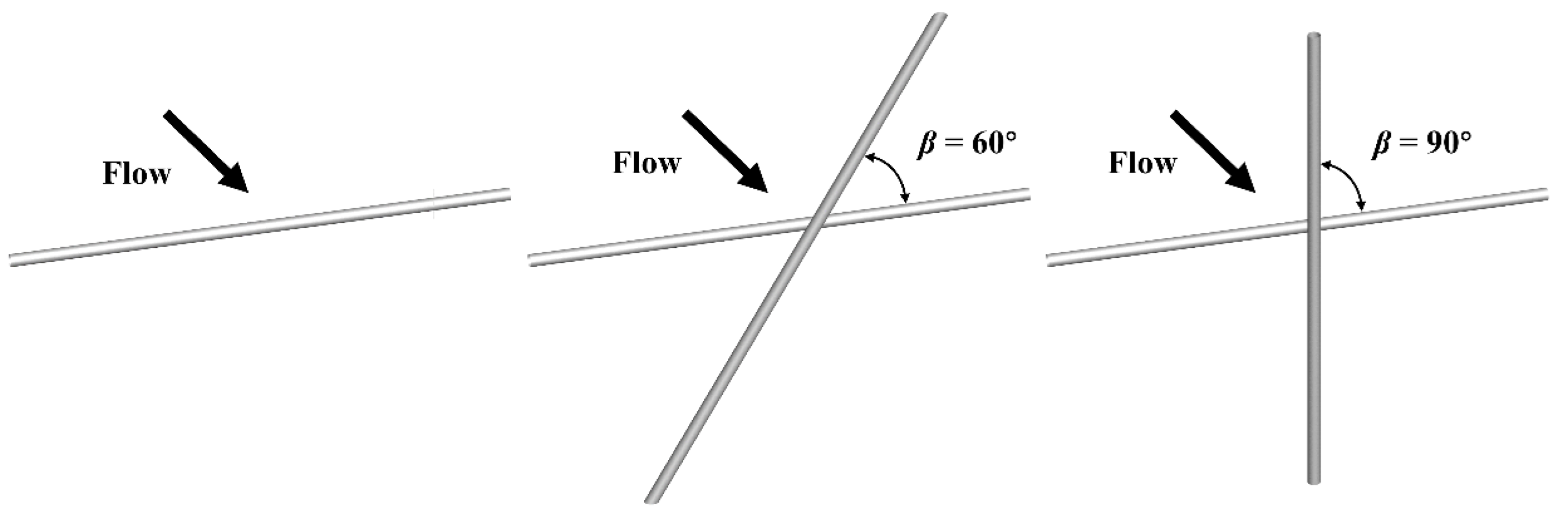
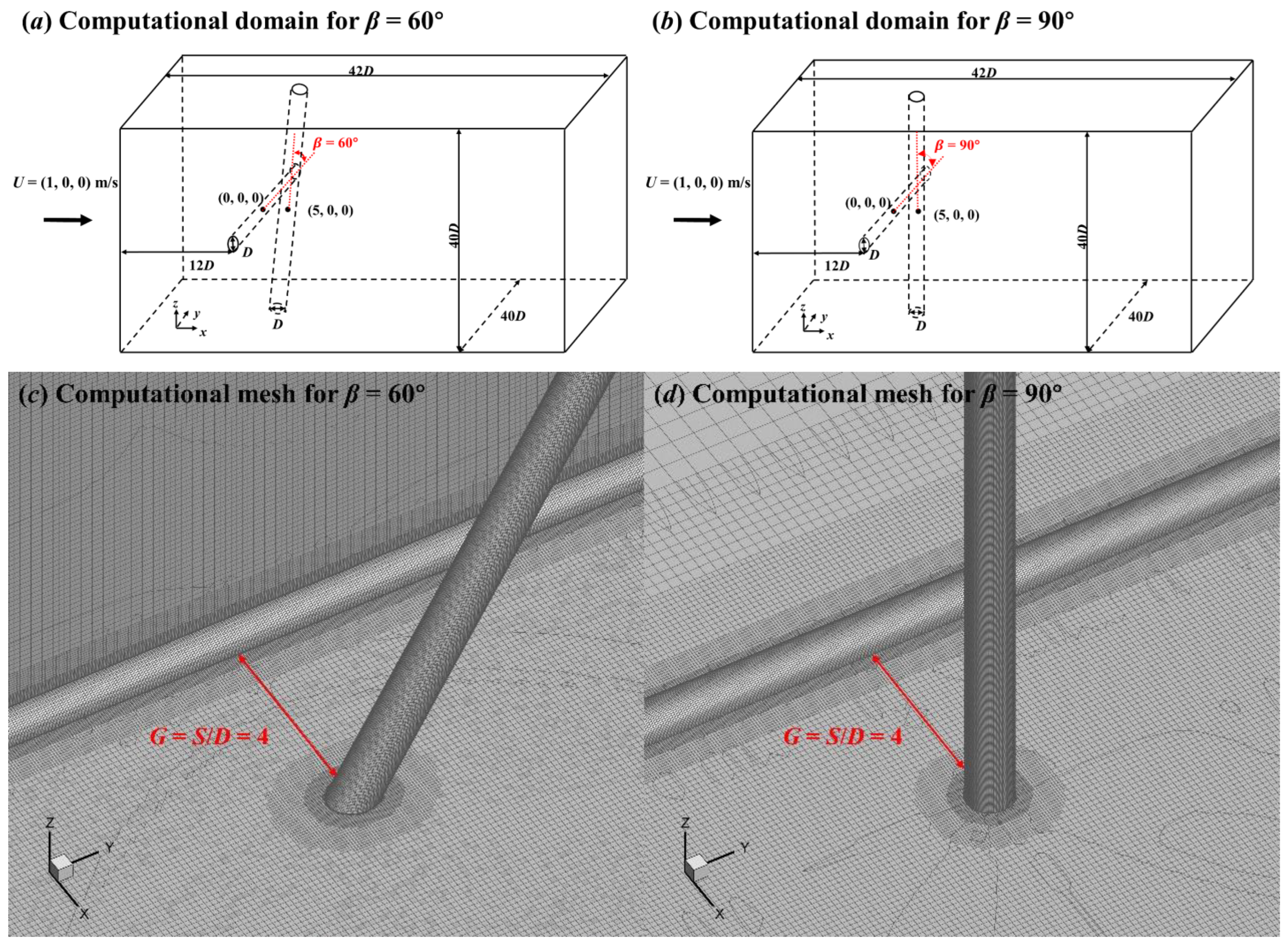
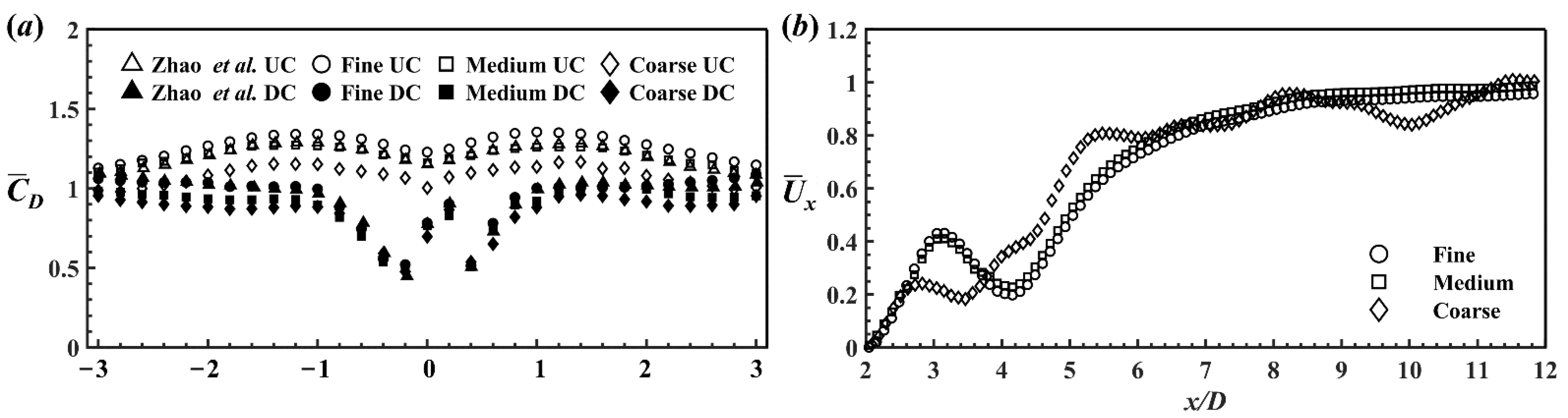
2. Overview of Numerical Simulation
3. Numerical Results
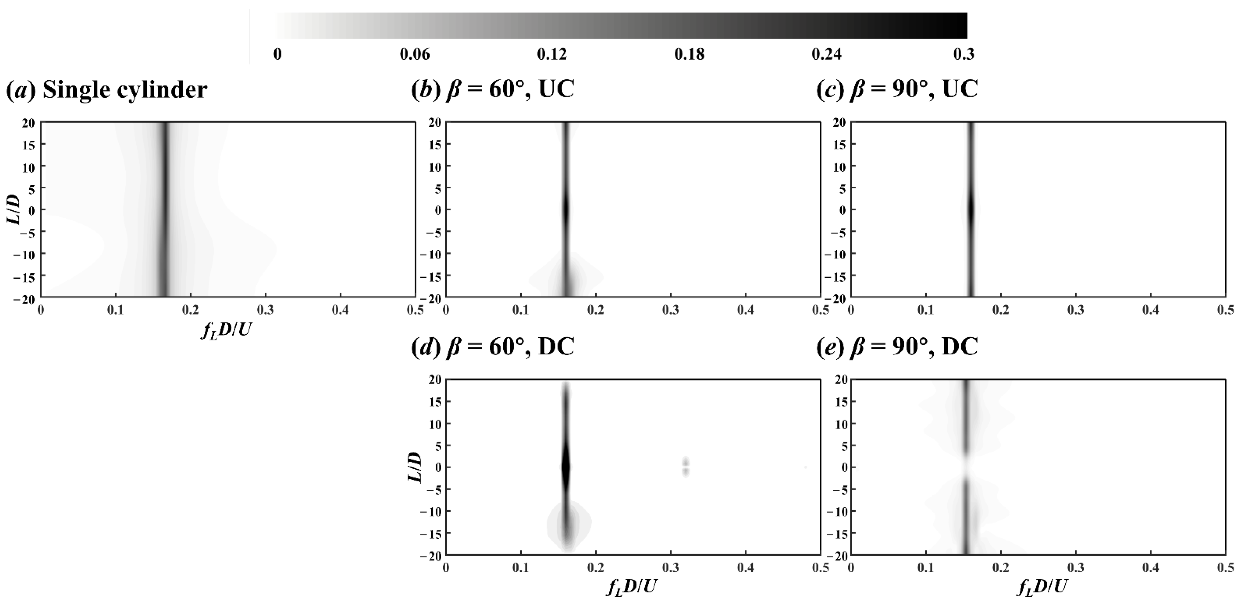
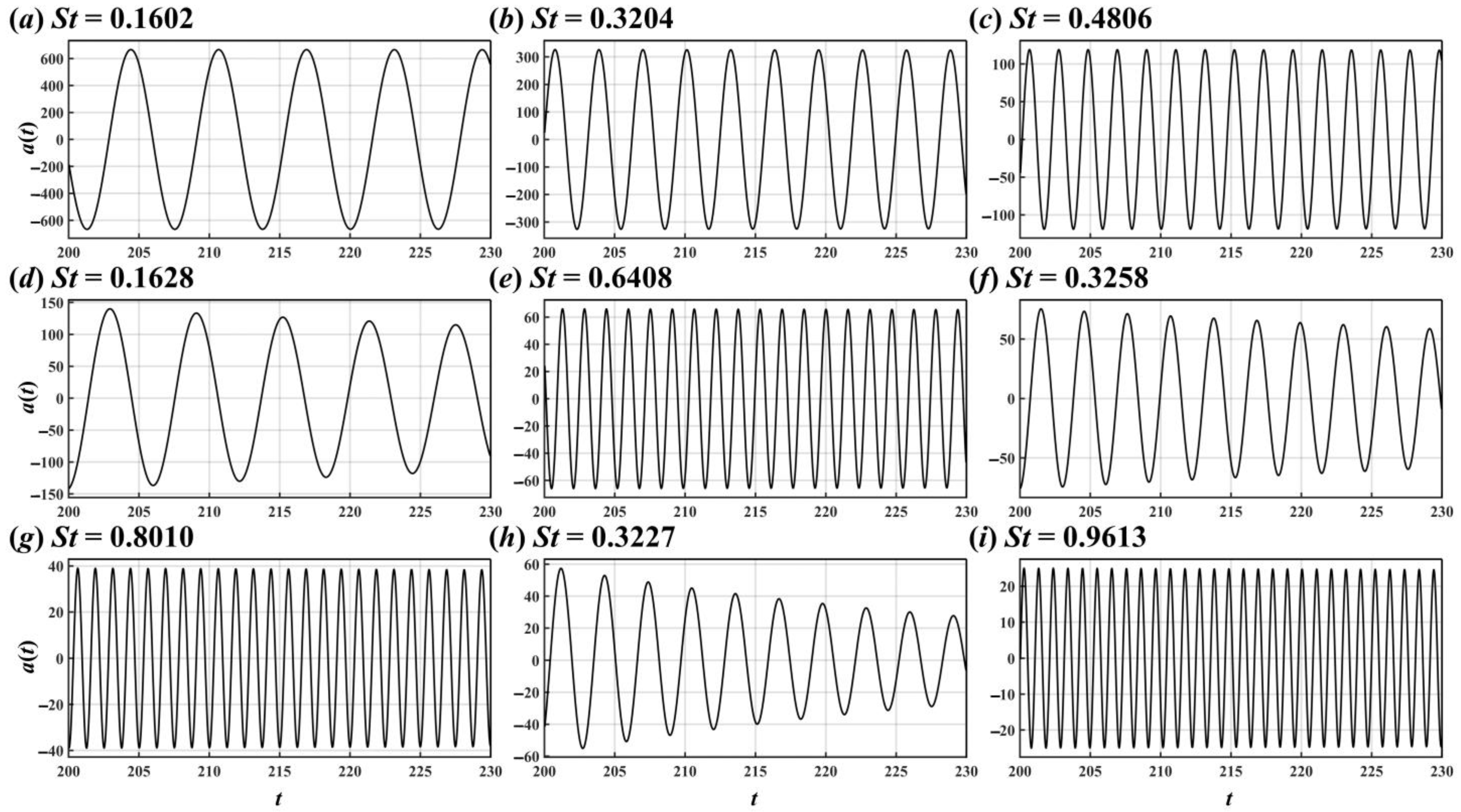
3.1. Lift Force Coefficient
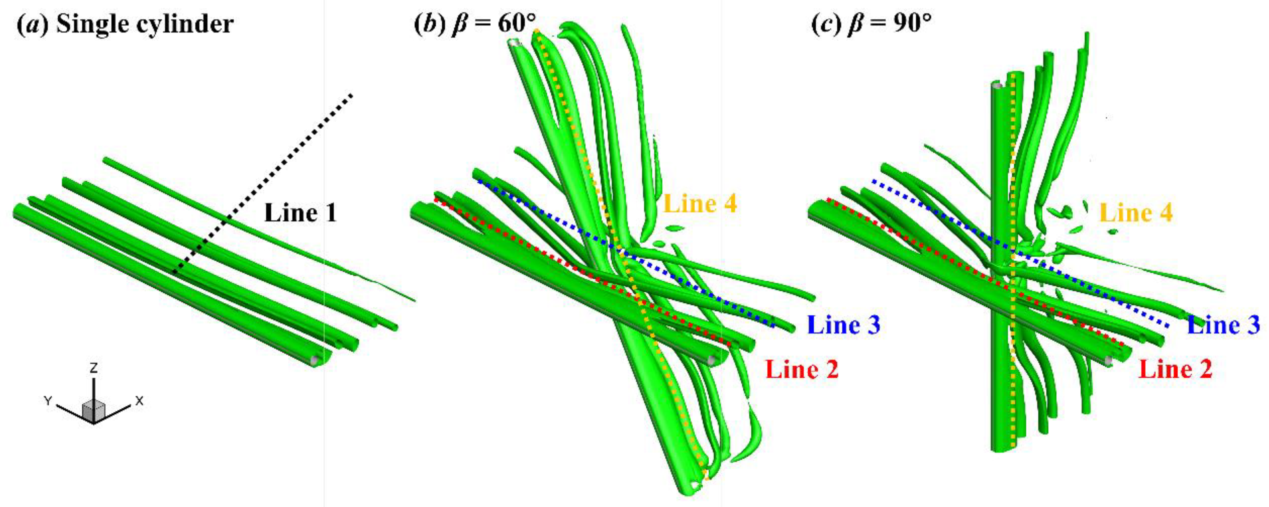
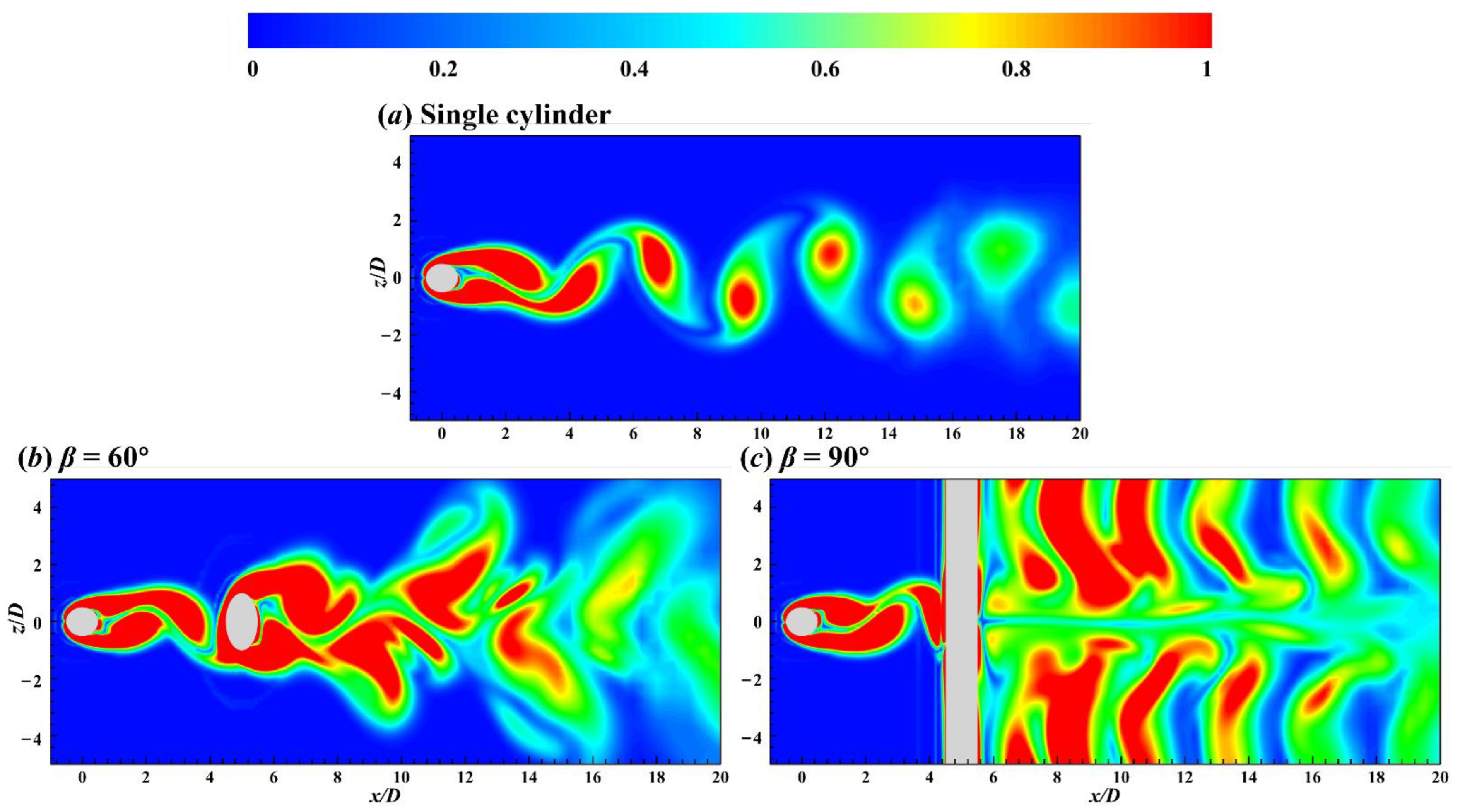
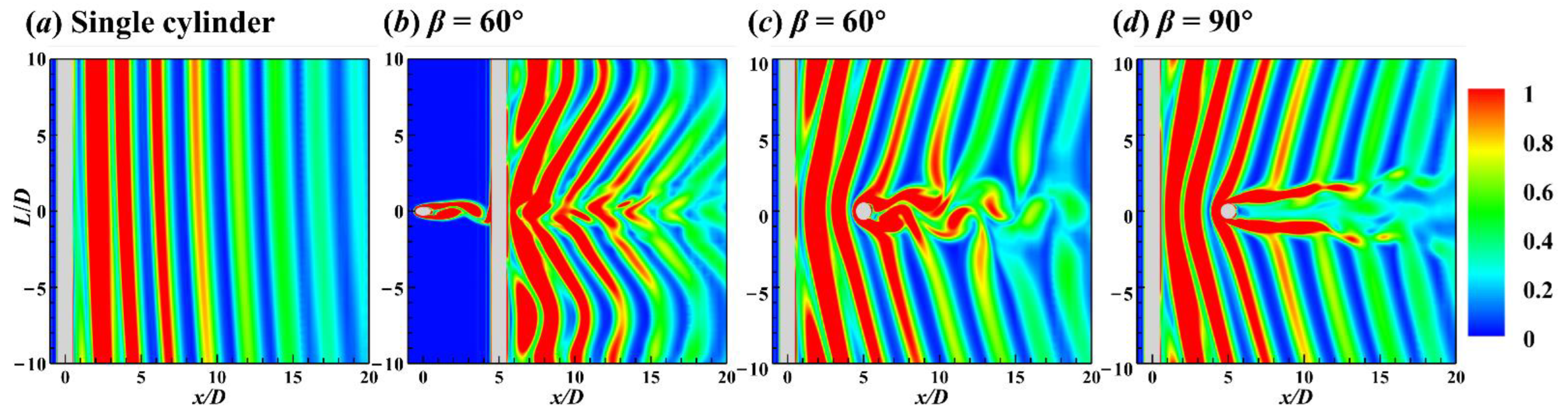
3.2. Flow Field
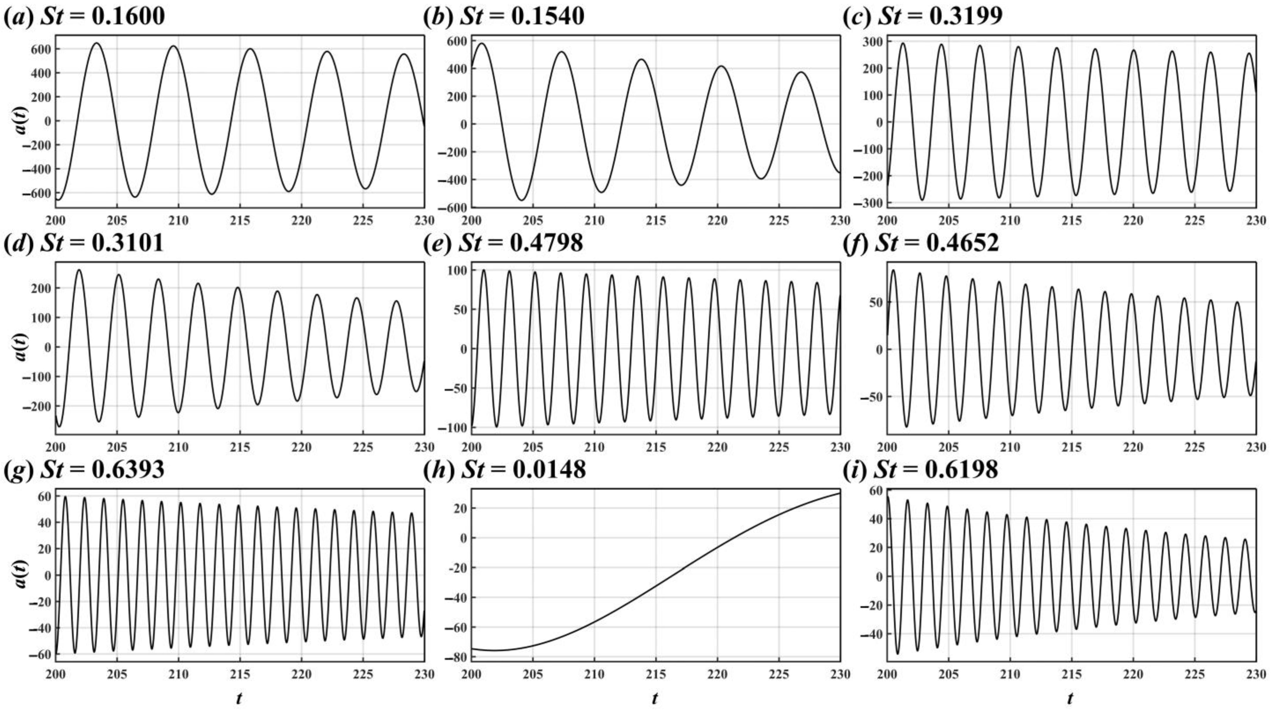
4. Modal Analysis
4.1. Methodology
4.1.1. POD
4.1.2. DMD
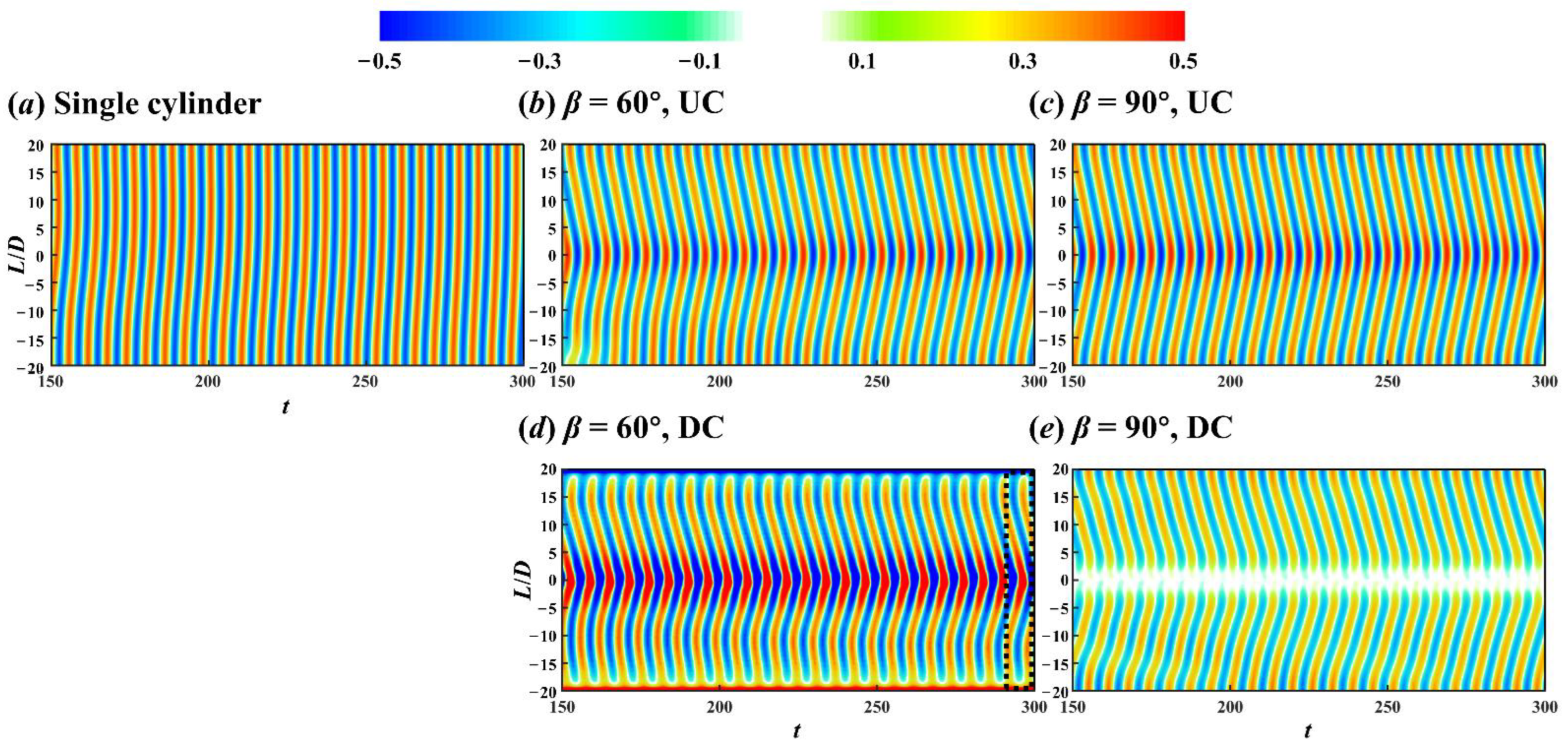
4.2. Raw Data
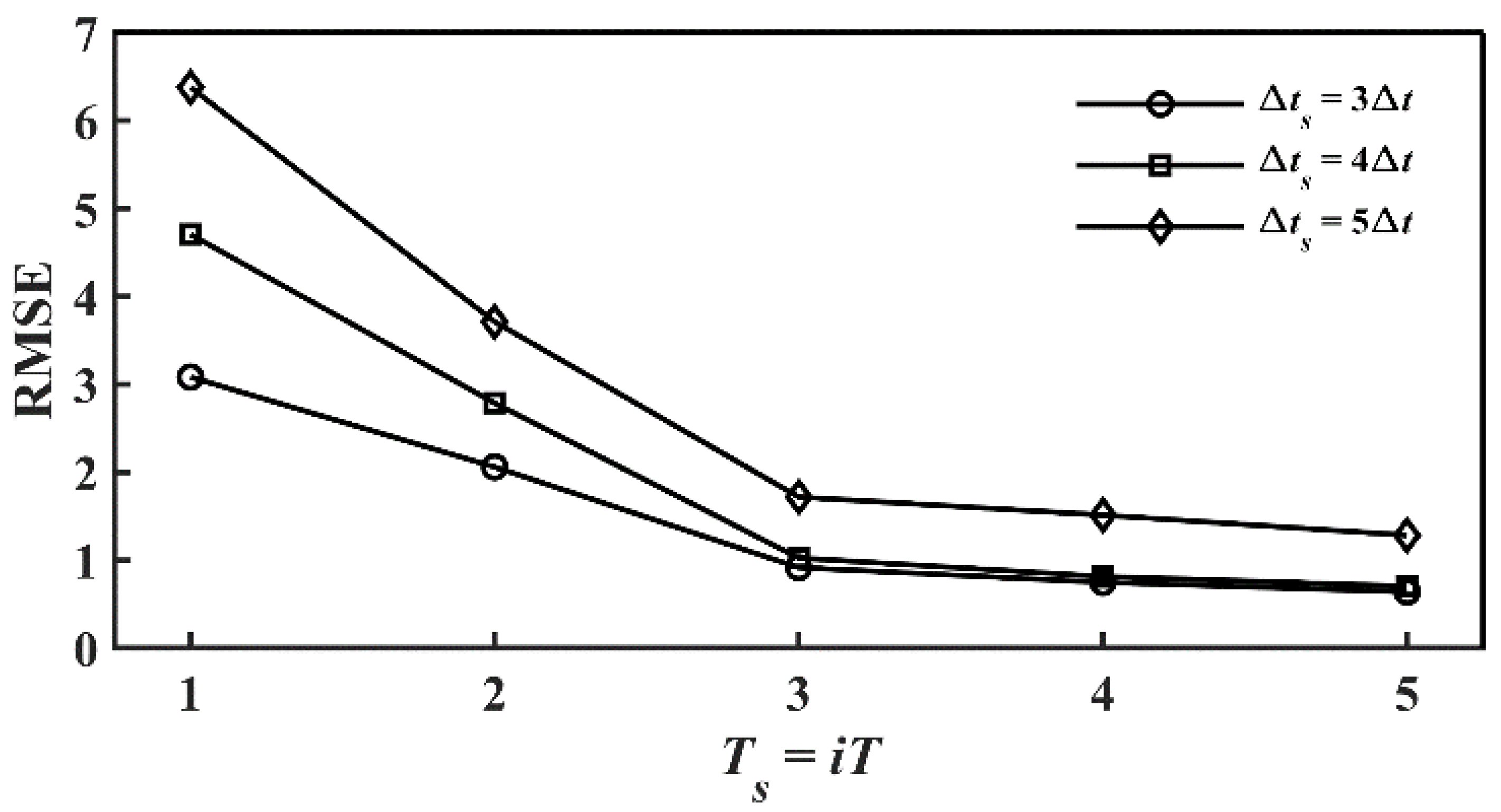
4.3. Modal Convergence Analysis
4.4. Modal Energy and Spectrum Statistics
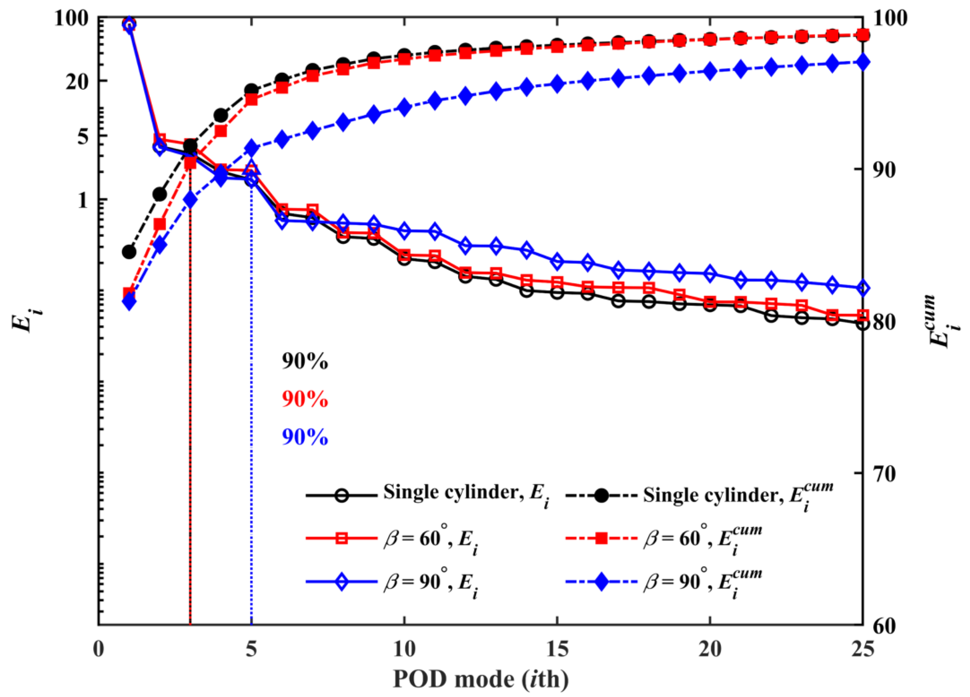
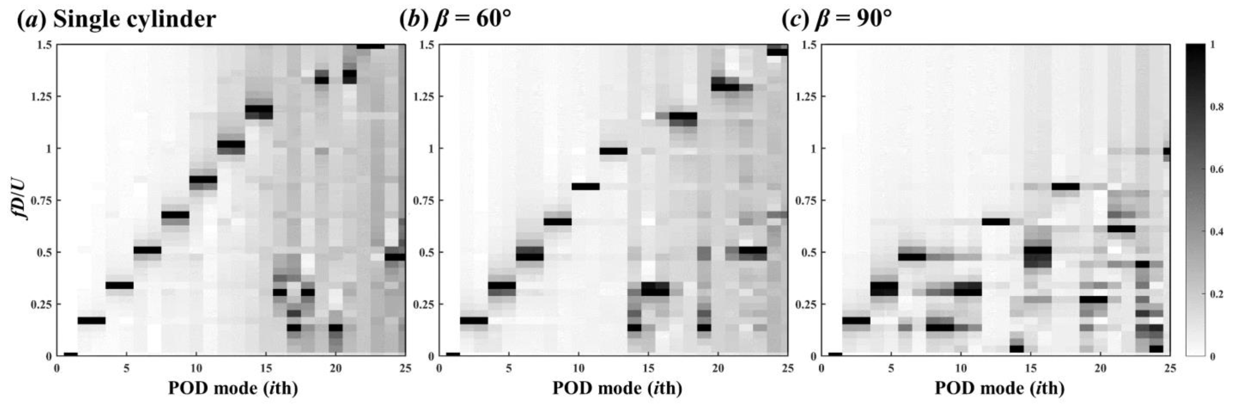
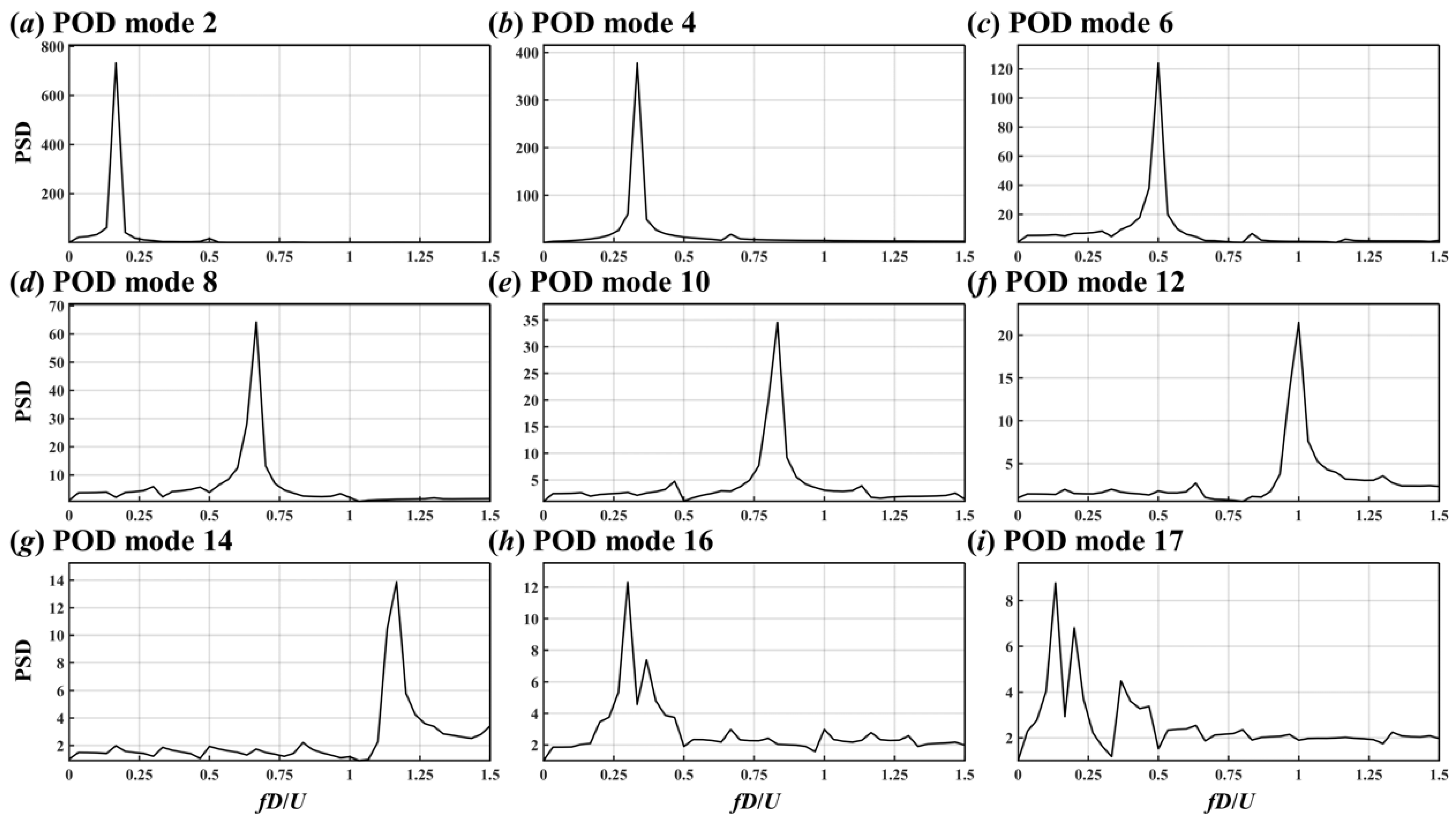
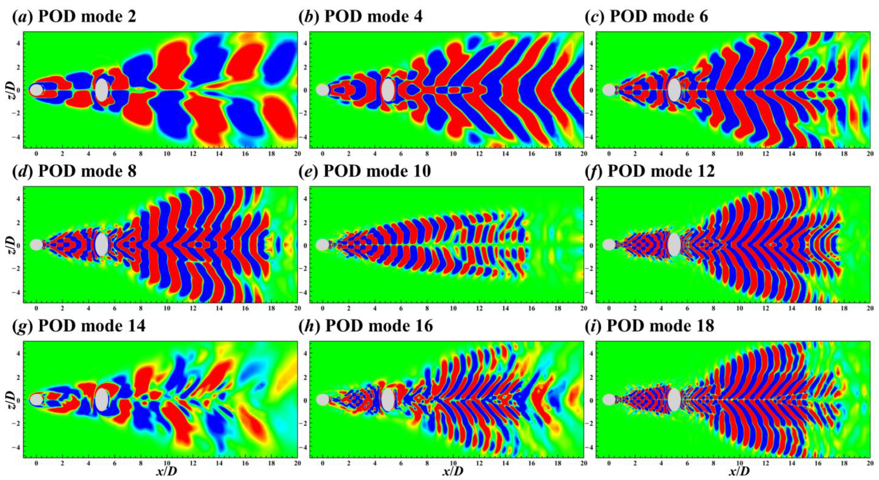
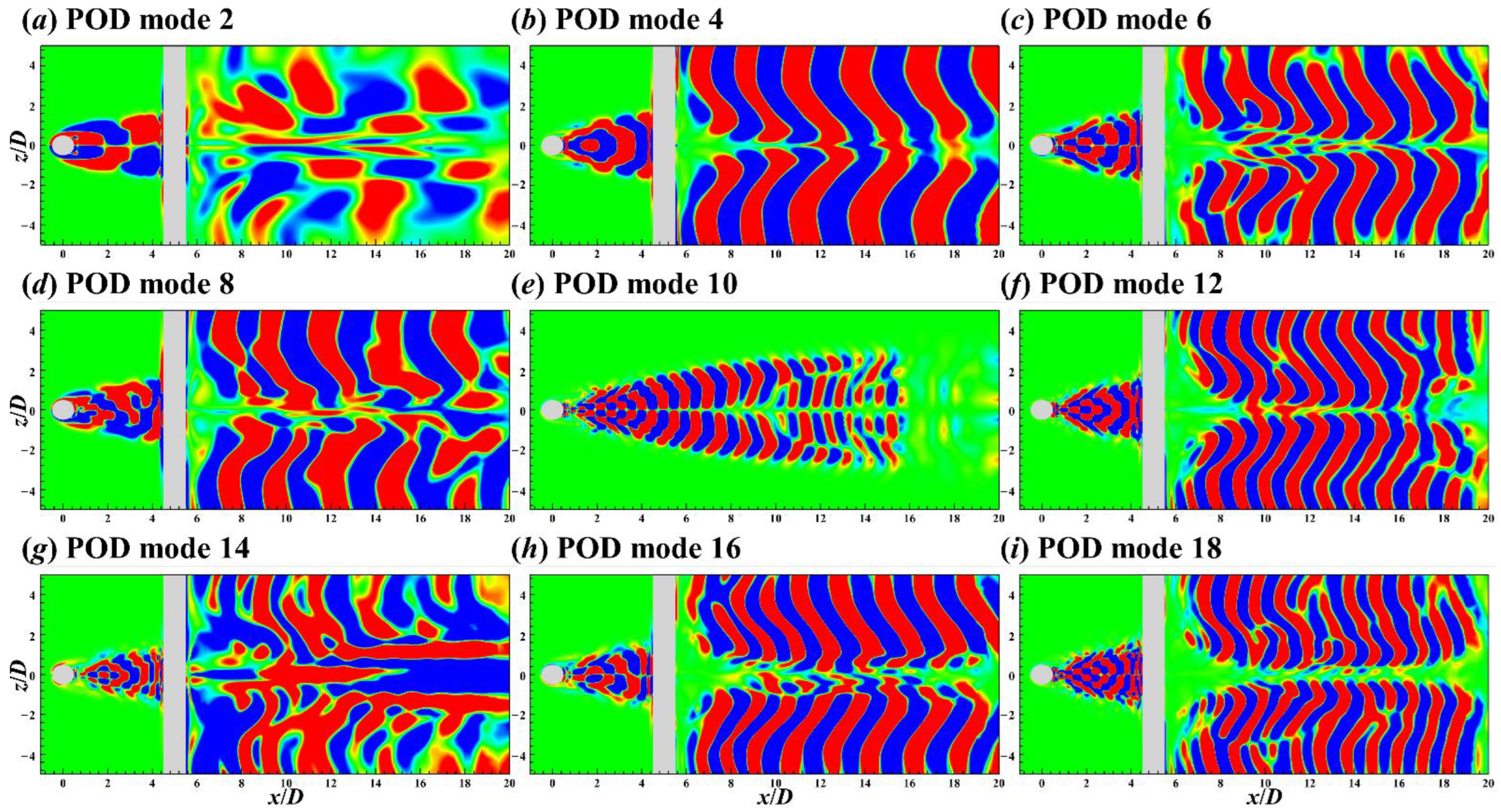
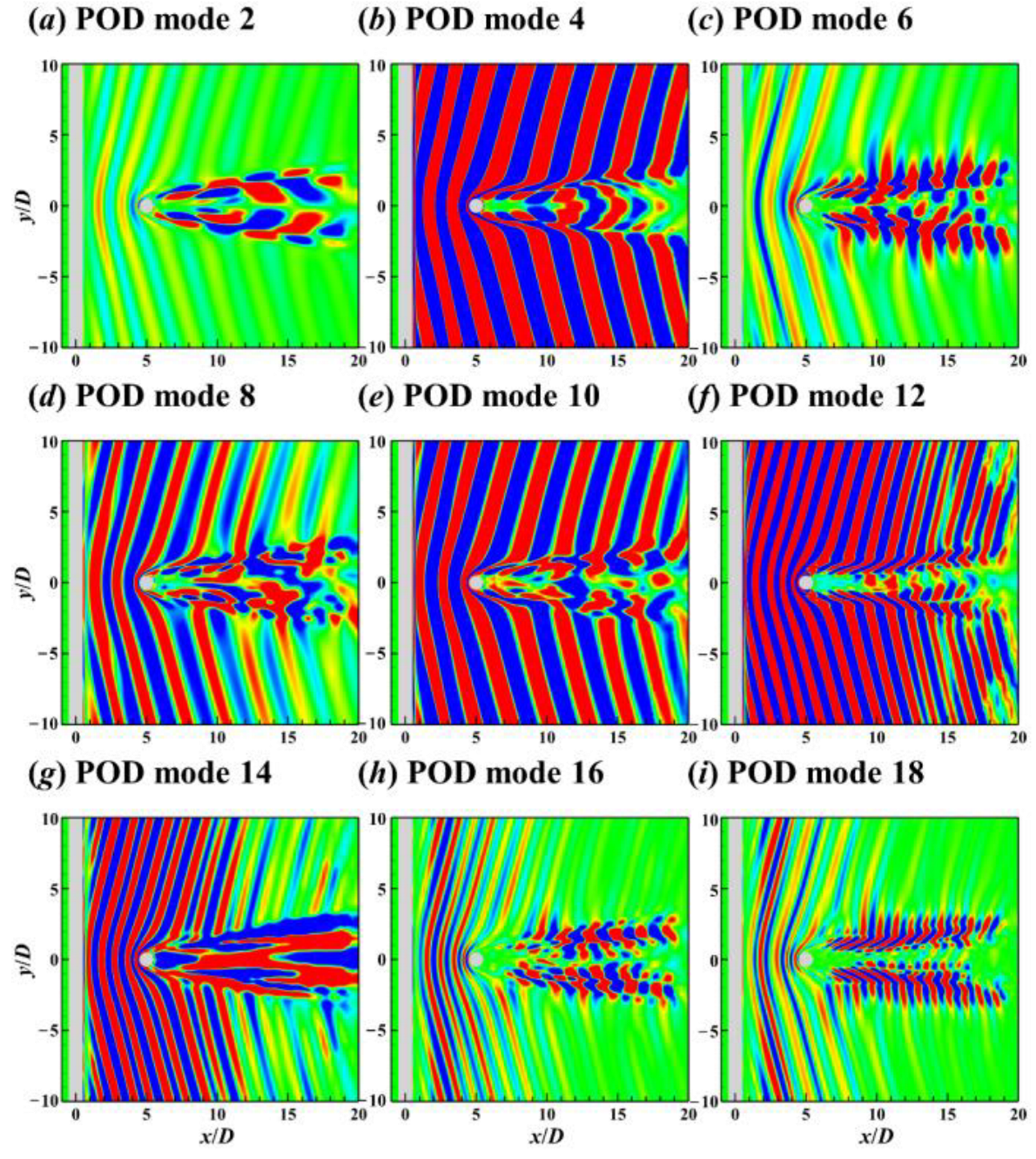
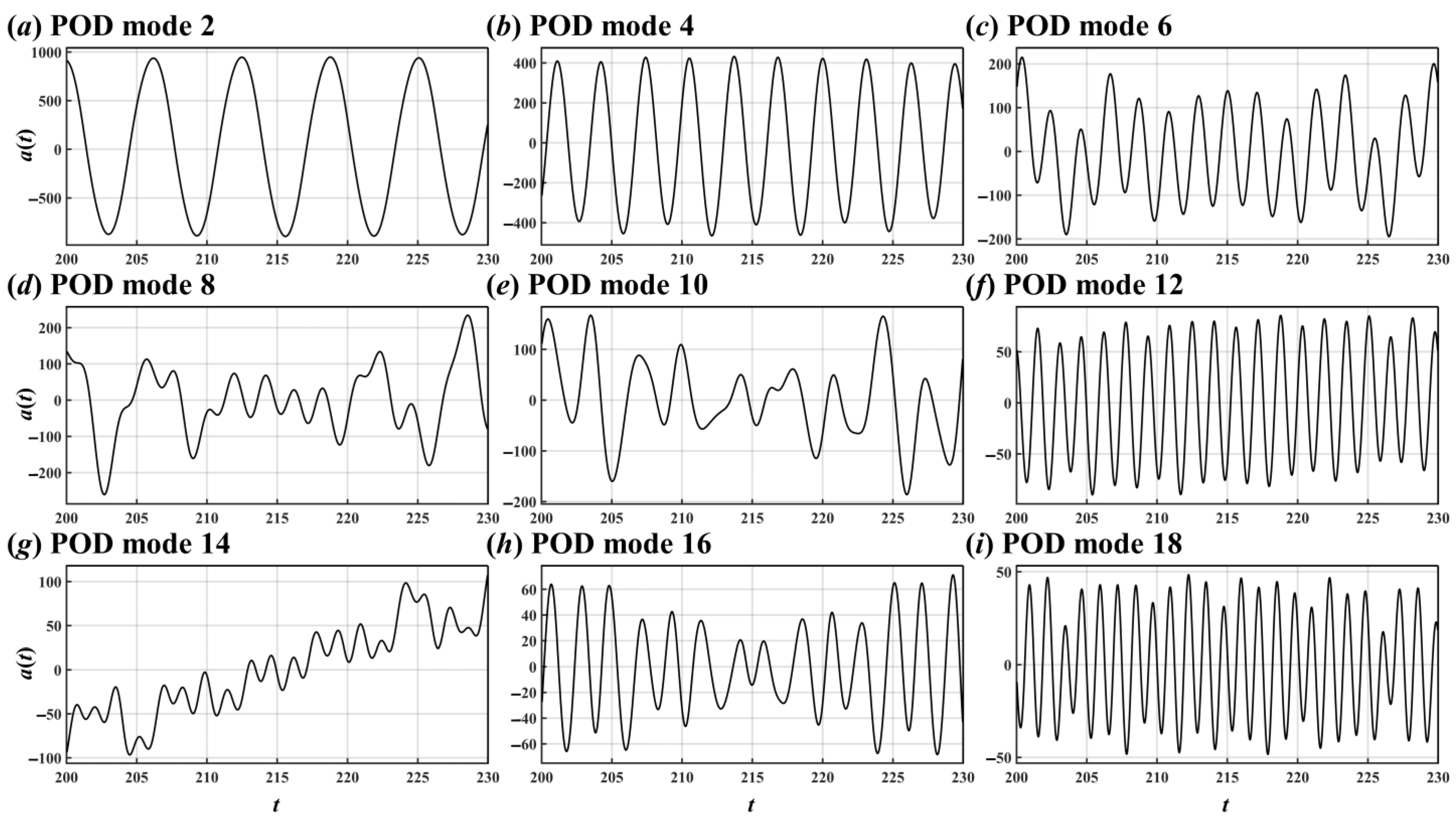
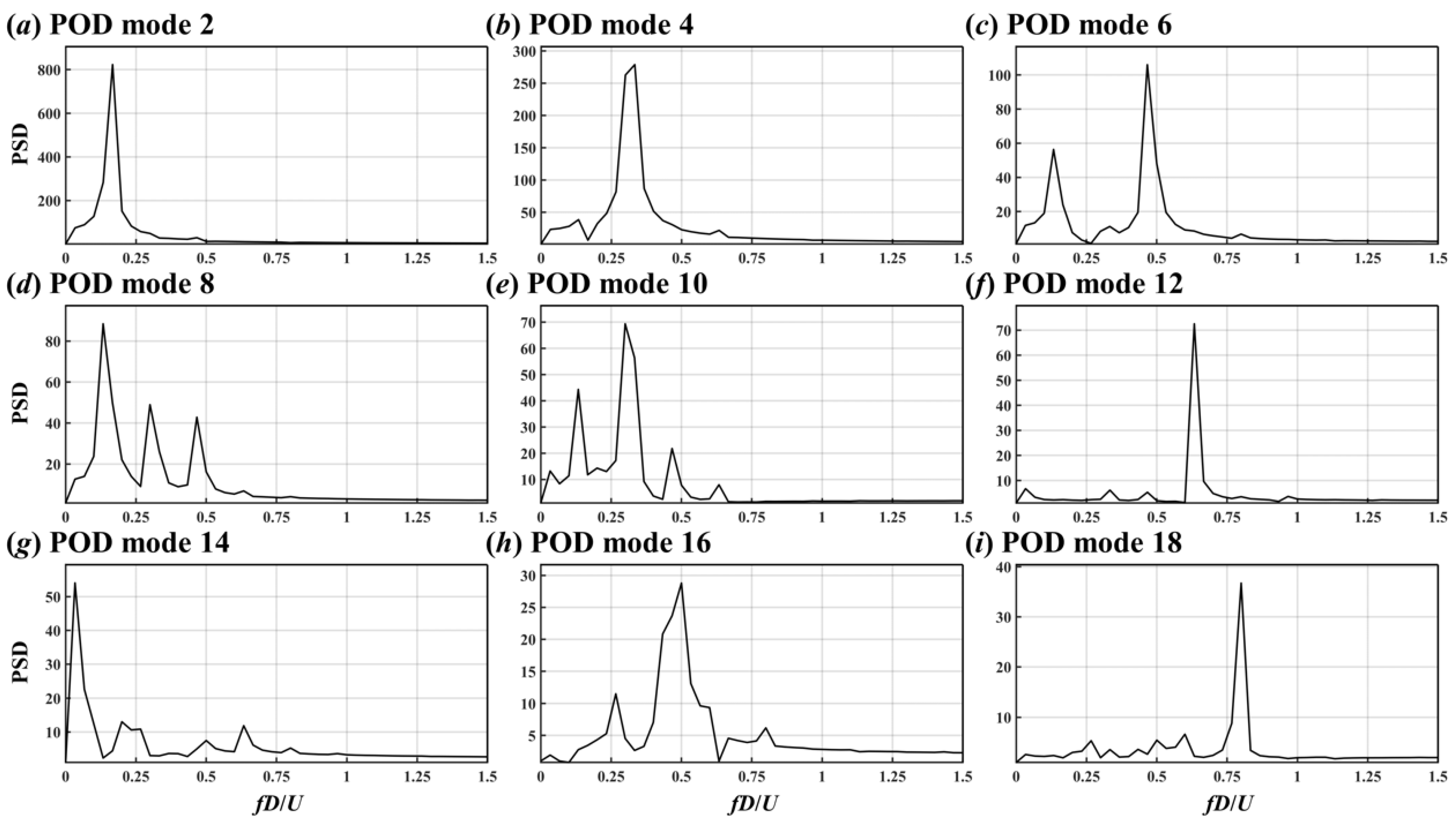
4.4.1. POD Modes
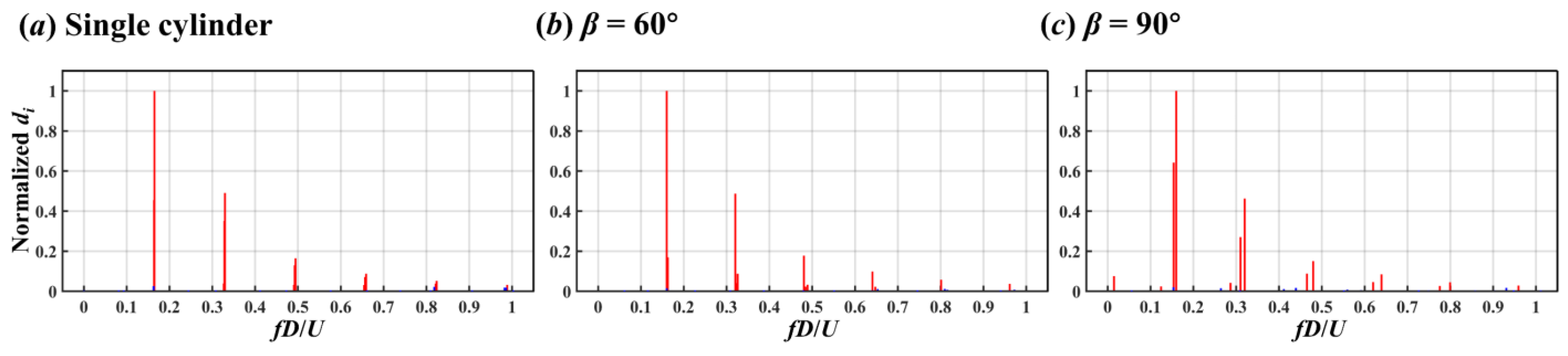
4.4.2. DMD Modes
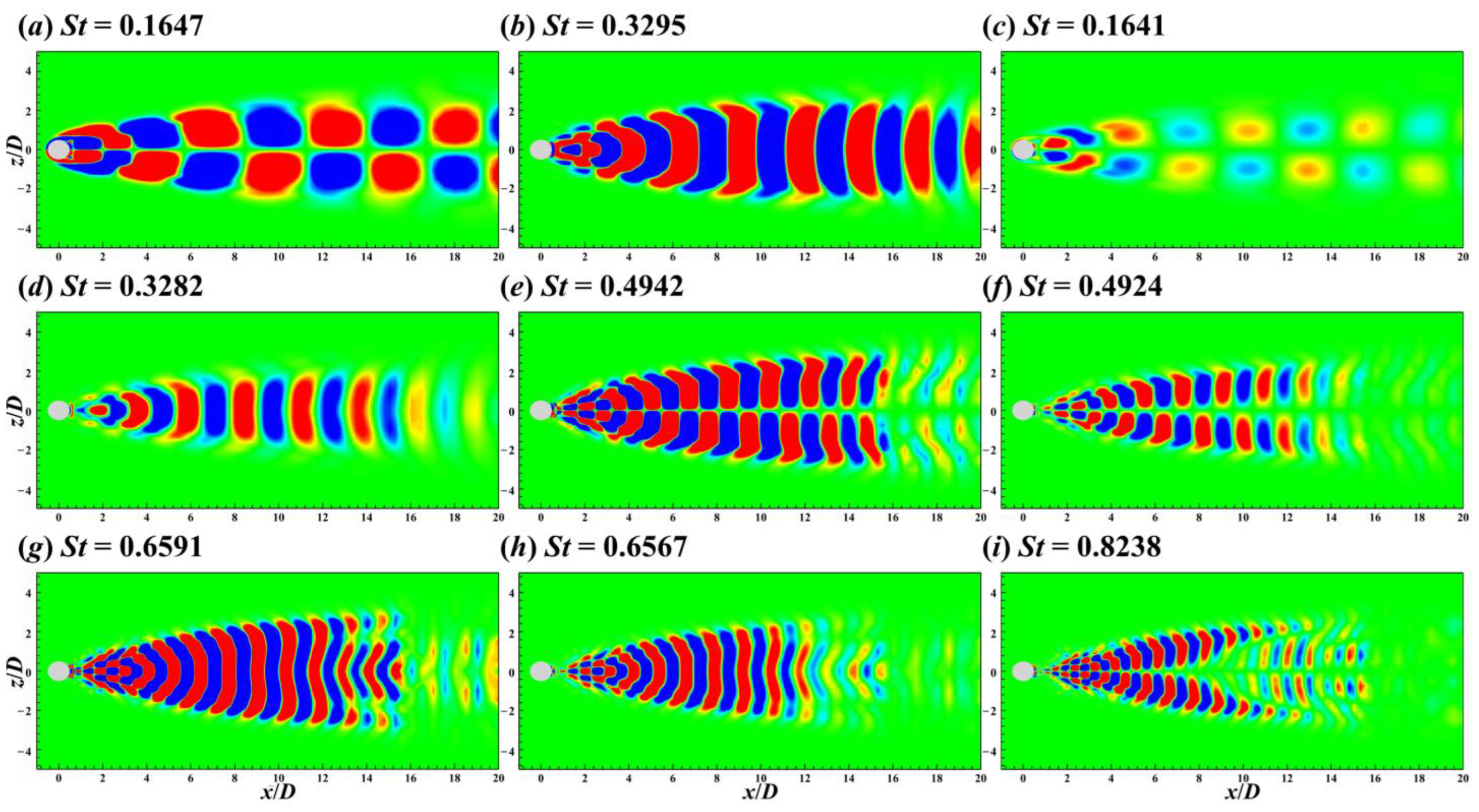
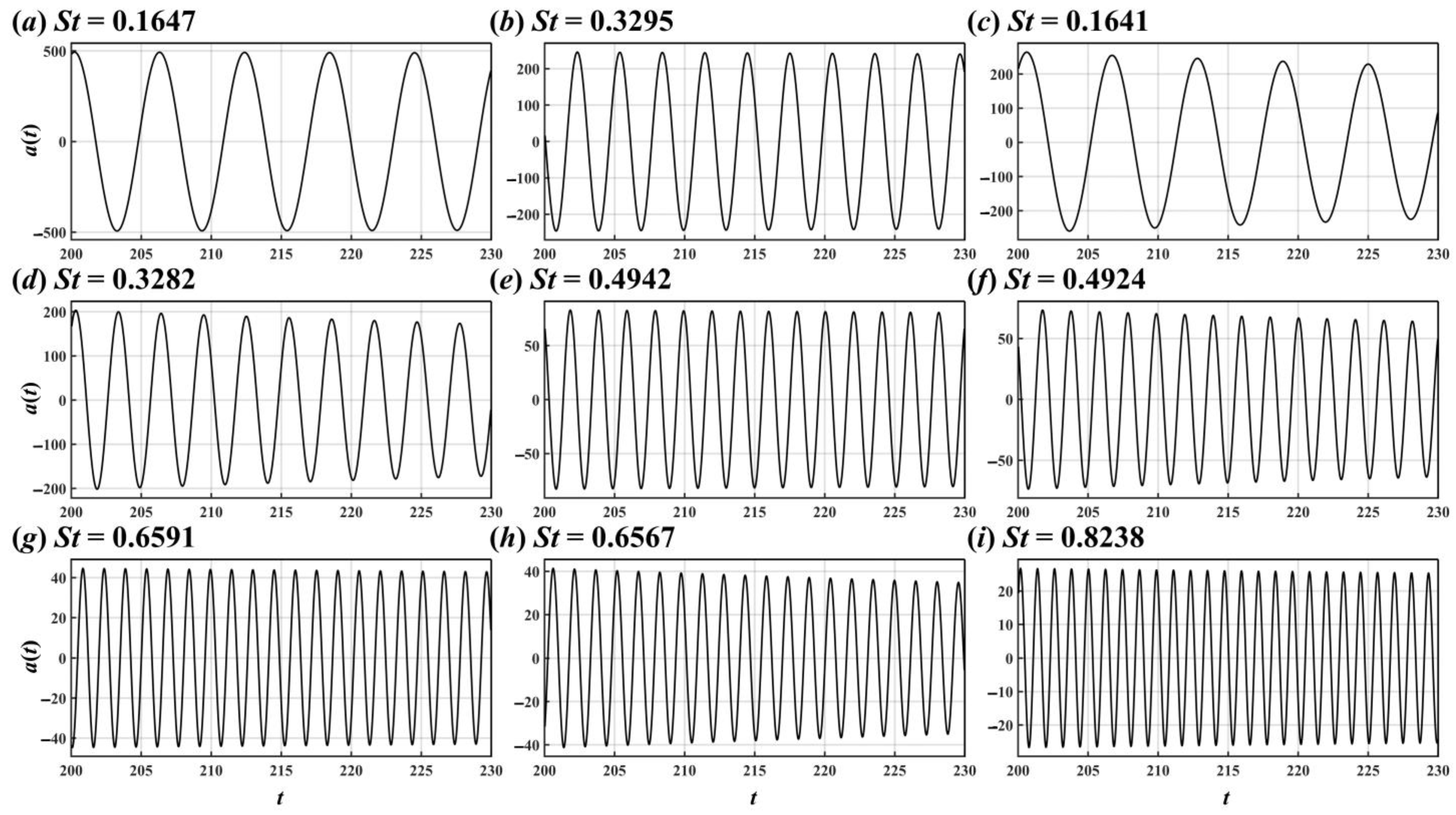
4.5. Modal Results
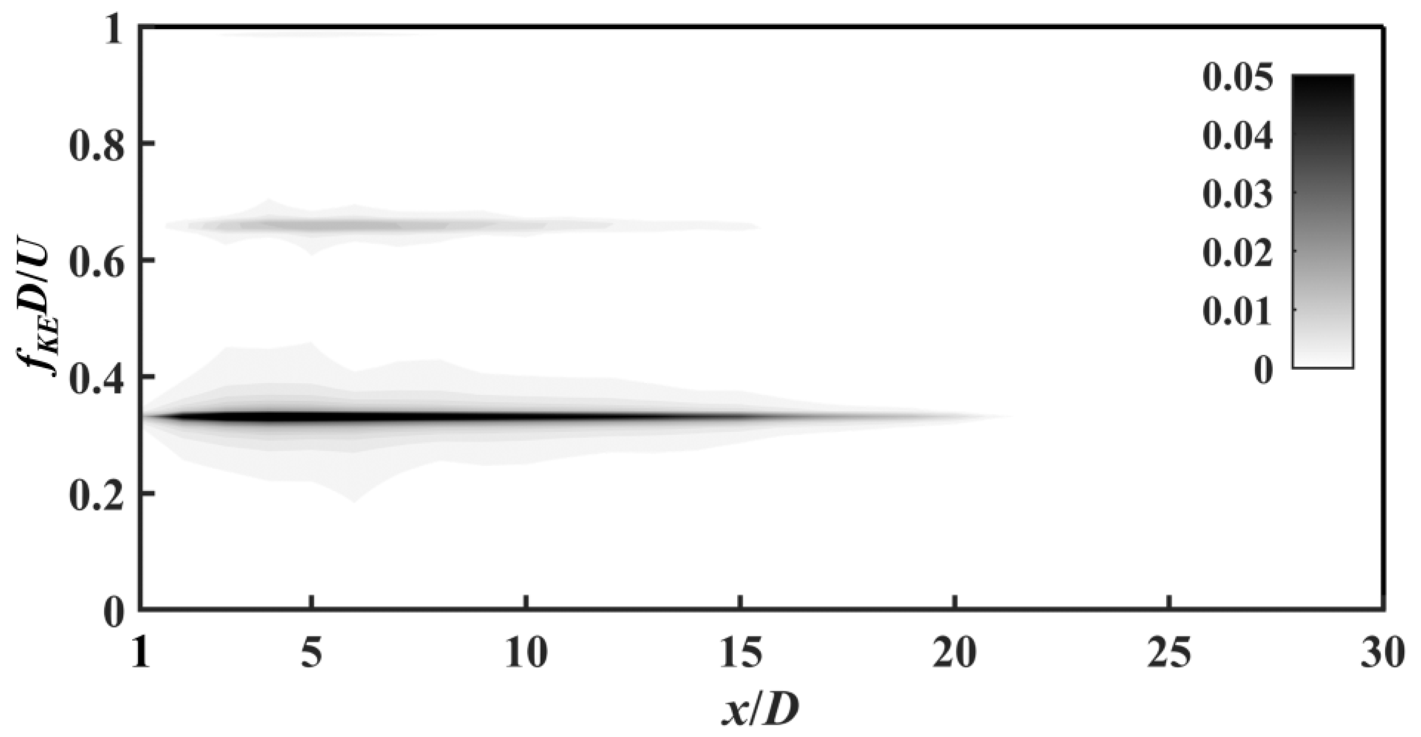
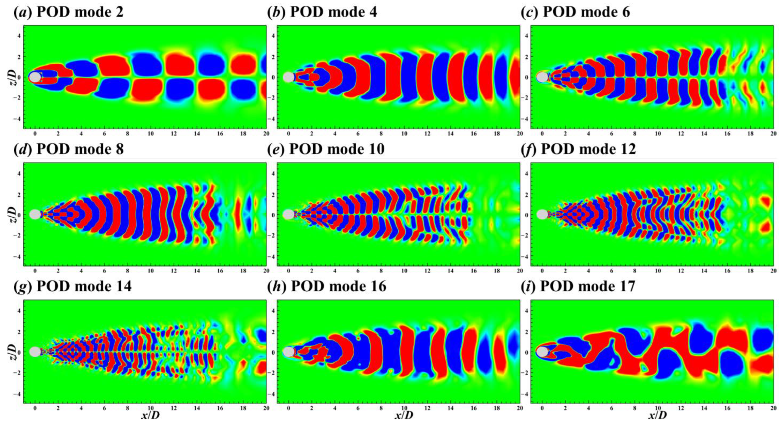
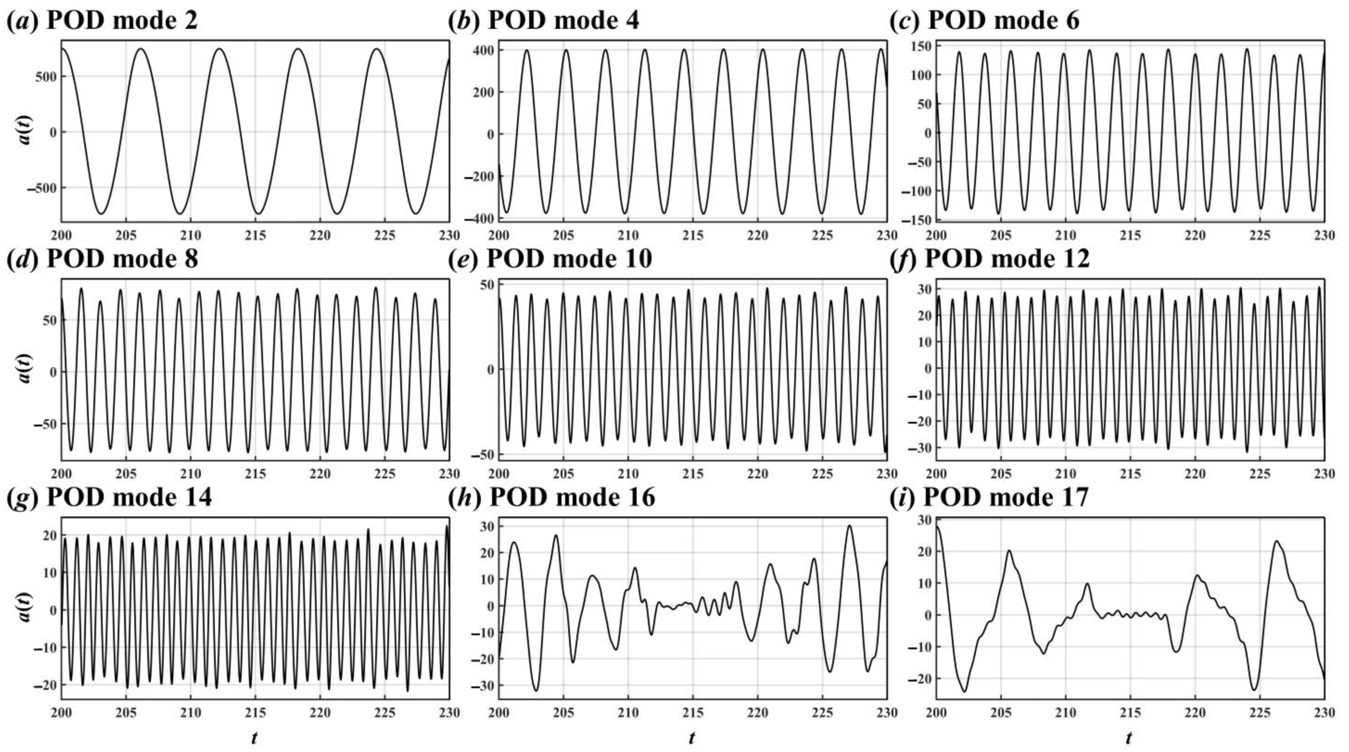
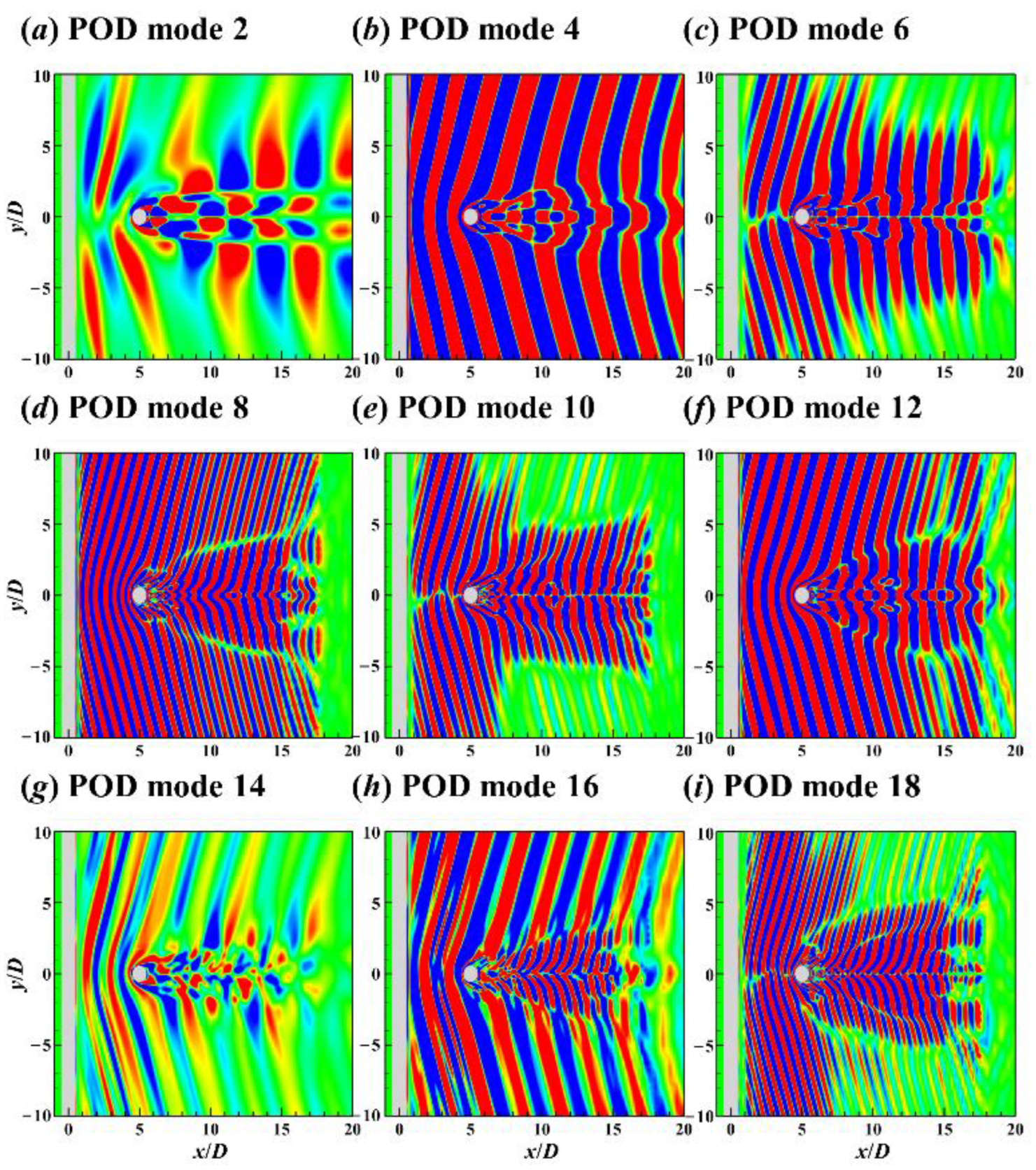
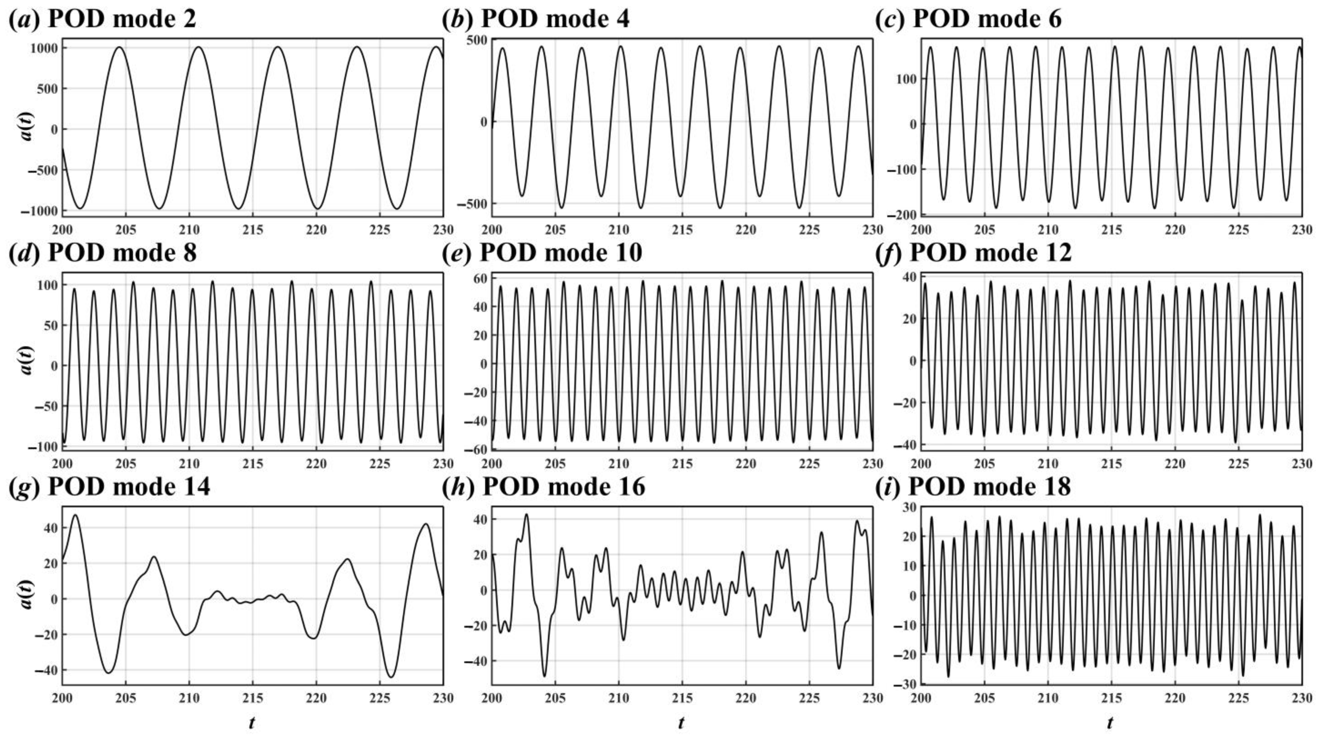
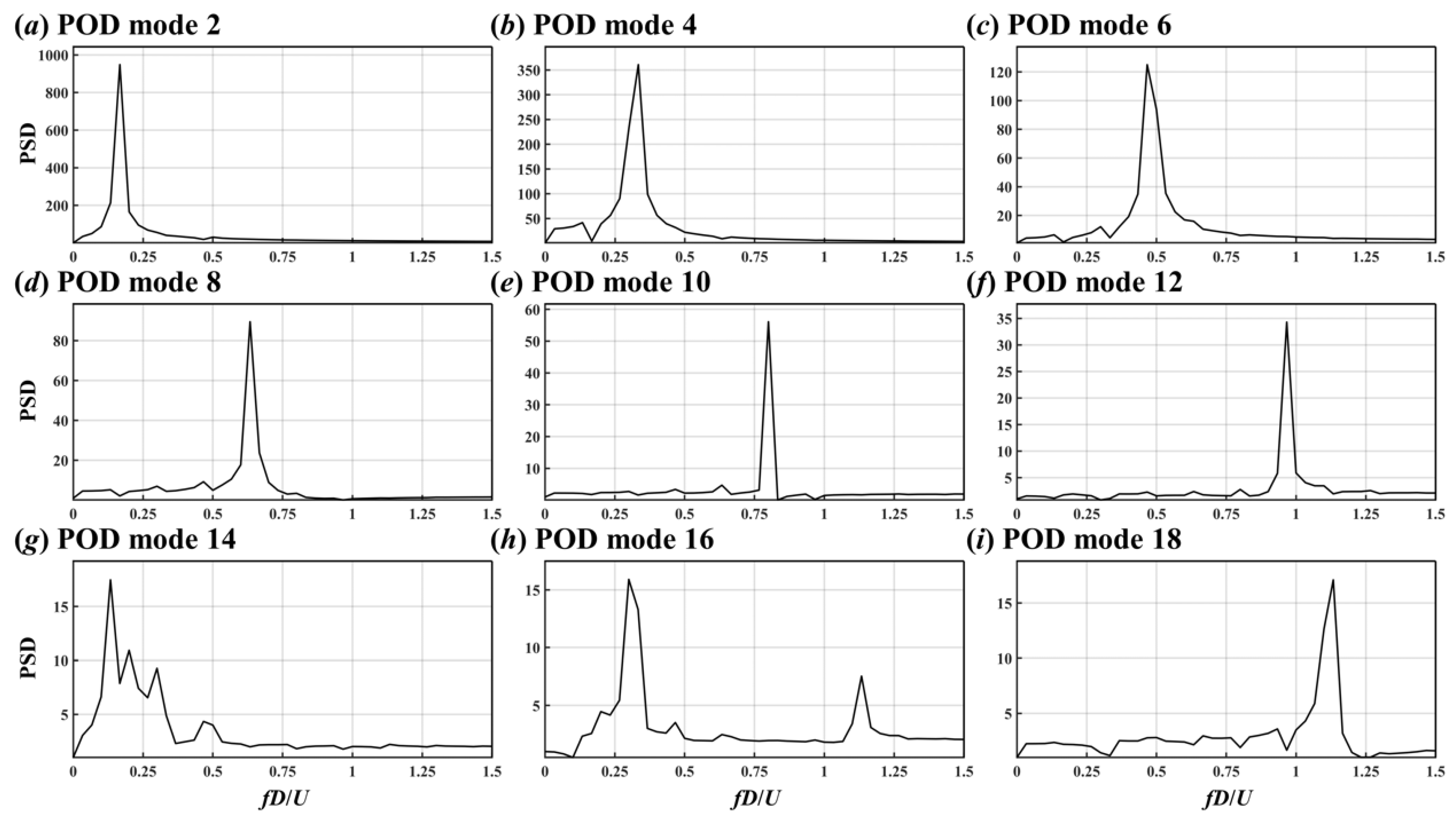
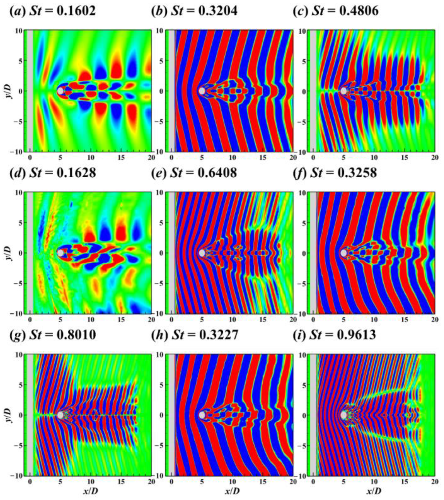
4.5.1. Single Cylinder
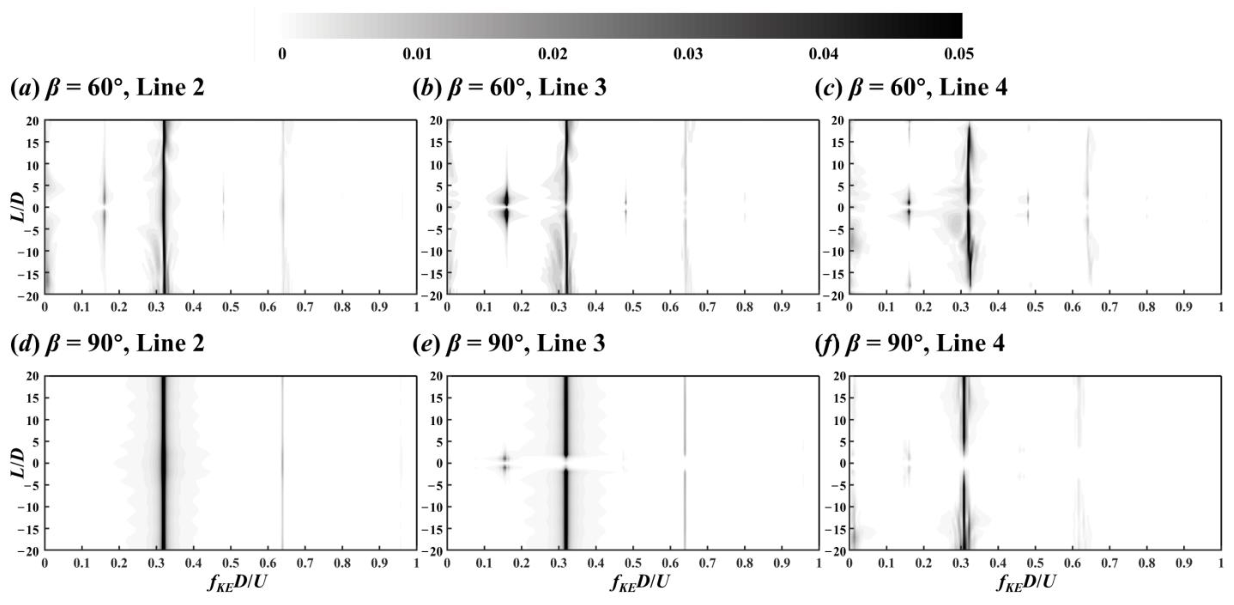
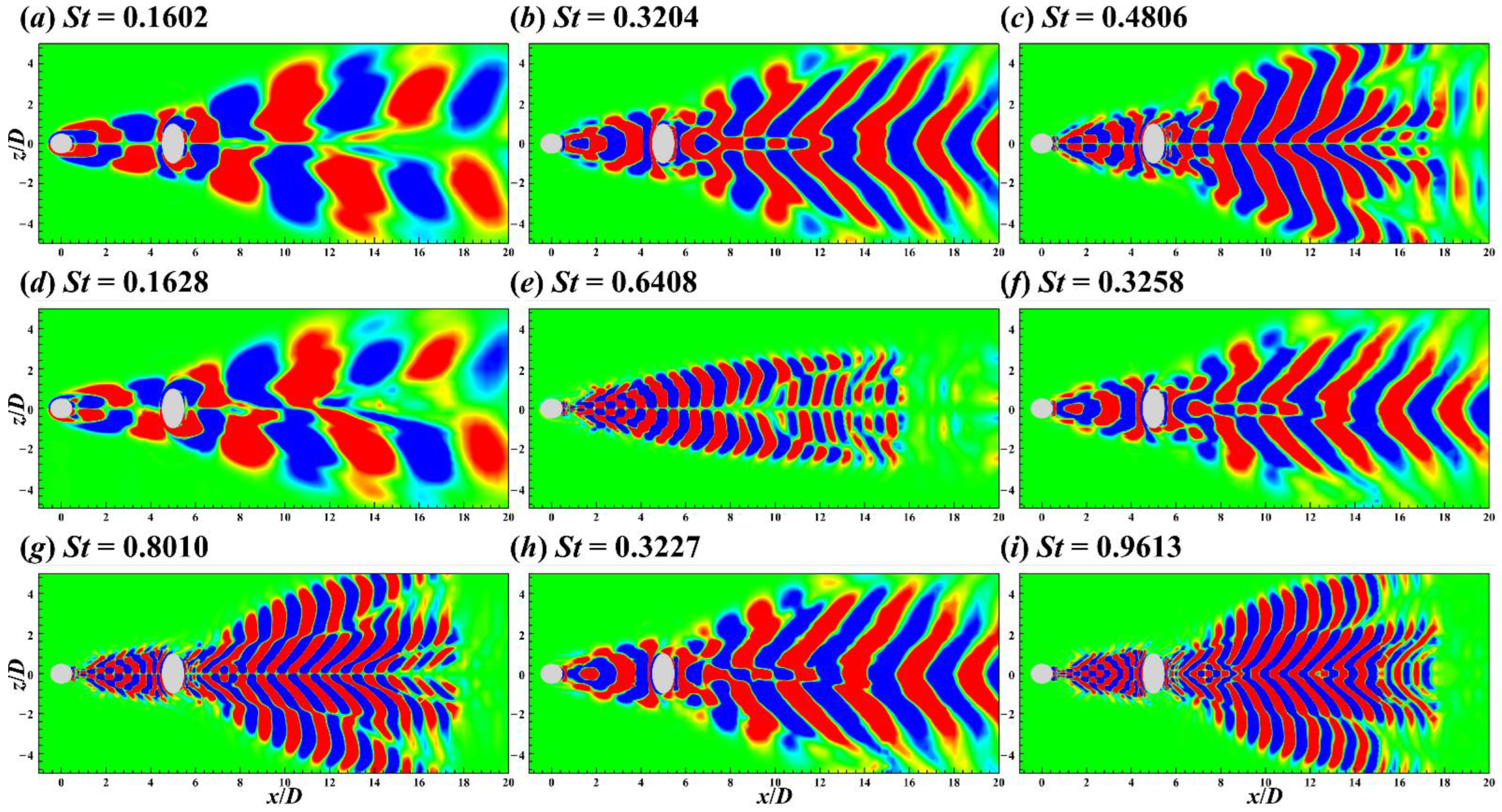
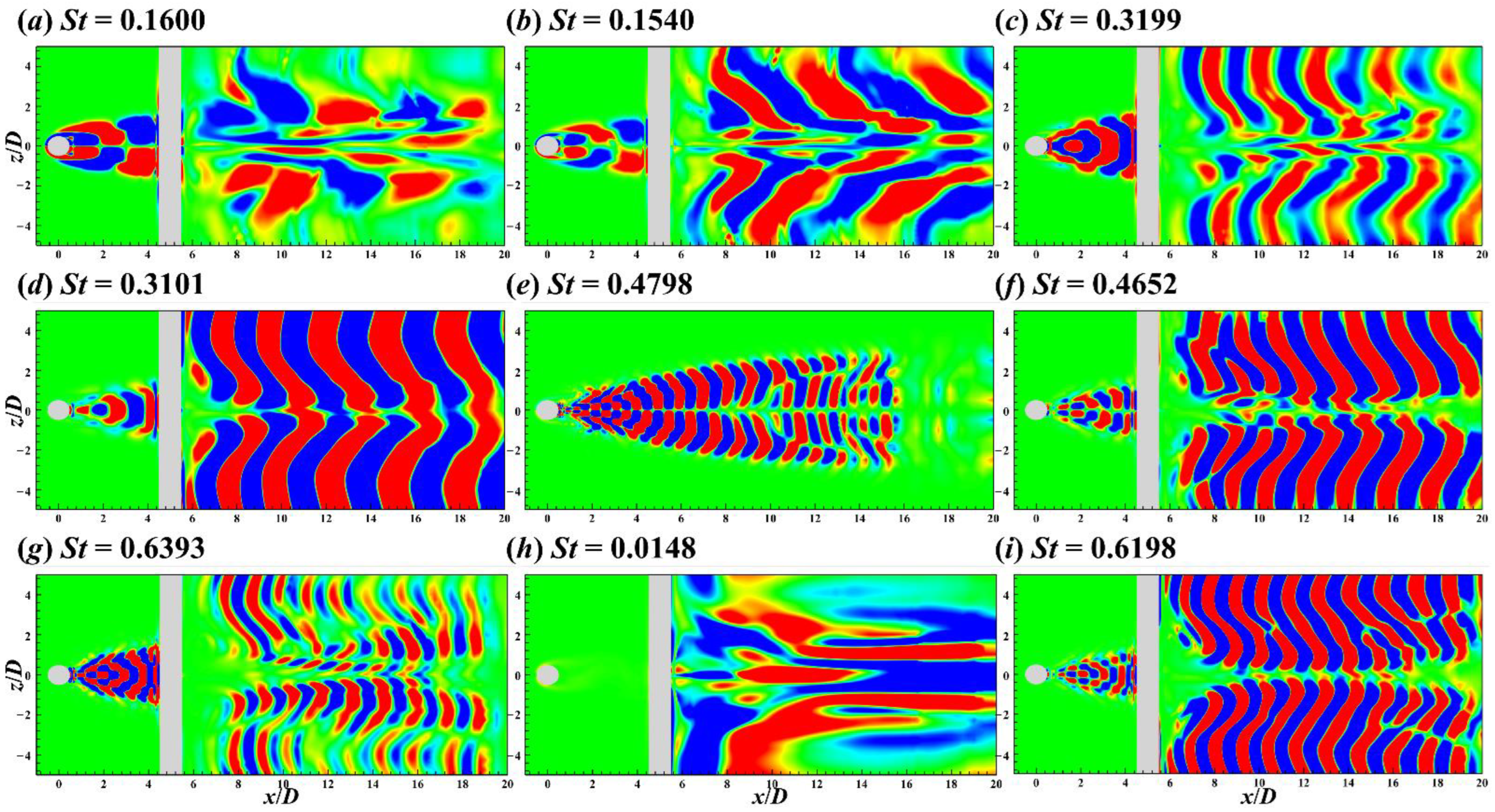
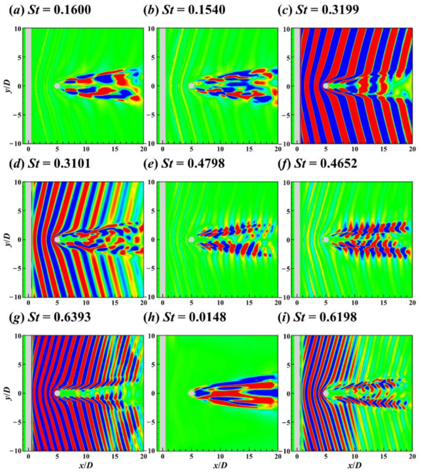
4.5.2. Two Crossing Cylinders in 60° Arrangement
4.5.3. Two Crossing Cylinders in 90° Arrangement
5. Summary
Author Contributions
Funding
Data Availability Statement
Conflicts of Interest
References
- Jauvtis, N.; Williamson, C.H.K. Vortex-induced vibration of a cylinder with two degrees of freedom. J. Fluids Struct. 2003, 17, 1035–1042. [Google Scholar] [CrossRef]
- Zhao, M.; Cheng, L.; Zhou, T. Direct numerical simulation of three-dimensional flow past a yawed circular cylinder of infinite length. J. Fluids Struct. 2009, 25, 831–847. [Google Scholar] [CrossRef]
- Deng, J.; Ren, A.L.; Shao, X.M. The flow between a stationary cylinder and a downstream elastic cylinder in cruciform arrangement. J. Fluids Struct. 2007, 23, 715–731. [Google Scholar] [CrossRef]
- Kato, N.; Koide, M.; Takahashi, T.; Shirakash, M. VIVs of a circular cylinder with a downstream strip-plate in cruciform arrangement. J. Fluids Struct. 2012, 30, 97–114. [Google Scholar] [CrossRef]
- Nguyen, T.; Koide, M.; Yamada, S.; Takahashi, T.; Shirakashi, M. Influence of mass and damping ratios on VIVs of a cylinder with a downstream counterpart in cruciform arrangement. J. Fluids Struct. 2012, 28, 40–55. [Google Scholar] [CrossRef]
- Sumner, D. Two circular cylinders in cross-flow: A review. J. Fluids Struct. 2010, 26, 849–899. [Google Scholar] [CrossRef]
- Tong, F.; Cheng, L.; Zhao, M. Numerical simulations of steady flow past two cylinders in staggered arrangements. J. Fluid Mech. 2015, 765, 114–149. [Google Scholar] [CrossRef]
- Zhao, M.; Lu, L. Numerical simulation of flow past two circular cylinders in cruciform arrangement. J. Fluid Mech. 2018, 848, 1013–1039. [Google Scholar] [CrossRef]
- Zhou, Y.; Mahbub, A.M. Wake of two interacting circular cylinders: A review. Int. J. Heat Fluid Flow 2016, 62, 510–537. [Google Scholar] [CrossRef]
- Taira, K.; Brunton, S.L.; Dawson, S.T.M.; Rowley, C.W.; Colonius, T.; McKeon, B.J.; Schmidt, O.T.; Gordeyev, S.; Theofilis, V.; Ukeiley, L.S. Modal Analysis of Fluid Flows: An Overview. Annu. Rev. Fluid Mech. 2017, 55, 4013–4041. [Google Scholar] [CrossRef] [Green Version]
- Lumley, J.L. Stochastic Tools in Turbulence; Academic Press: Cambridge, MA, USA, 2008. [Google Scholar]
- Schmid, P.J. Dynamic Mode Decomposition of numerical and experimental data. J. Fluid Mech. 2010, 656, 5–28. [Google Scholar] [CrossRef] [Green Version]
- Sakai, M.; Sunada, Y.; Imamura, T.; Rinoie, K. Experimental and Numerical Studies on Flow behind a Circular Cylinder Based on POD and DMD. Trans. Jpn. Soc. Aeronaut. Space Sci. 2015, 58, 100–107. [Google Scholar] [CrossRef] [Green Version]
- Tu, J.H.; Rowley, C.W.; Kutz, J.N.; Shang, J.K. Spectral analysis of fluid flows using sub-Nyquist-rate PIV data. Exp. Fluids 2014, 55, 1805. [Google Scholar] [CrossRef] [Green Version]
- Wang, H.F.; Cao, H.L.; Zhou, Y. POD analysis of a finite-length cylinder near wake. Exp. Fluids 2014, 55, 1790. [Google Scholar] [CrossRef]
- Bagheri, S. Koopman-mode decomposition of the cylinder wake. J. Fluid Mech. 2013, 726, 596–623. [Google Scholar] [CrossRef]
- Bai, H.L.; Alam, M.M.; Gao, N.; Lin, Y.F. The near wake of sinusoidal wavy cylinders: Three-dimensional POD analyses. Int. J. Heat Fluid Flow 2019, 75, 256–277. [Google Scholar] [CrossRef]
- Chen, K.K.; Tu, J.H.; Rowley, C.W. Variants of Dynamic Mode Decomposition: Boundary Condition, Koopman, and Fourier Analyses. J. Nonlinear Sci. 2012, 22, 887–915. [Google Scholar] [CrossRef]
- Naderi, M.H.; Eivazi, H.; Esfahanian, V. New method for dynamic mode decomposition of flows over moving structures based on machine learning (hybrid dynamic mode decomposition). Phys. Fluids 2019, 31, 127102. [Google Scholar] [CrossRef]
- Scherl, I.; Strom, B.; Shang, J.; Williams, O.; Polagye, B.; Brunton, S. Robust principal component analysis for modal decomposition of corrupt fluid flows. Phys. Rev. Fluid 2020, 5, 054401. [Google Scholar] [CrossRef]
- Zhao, Y.; Zhao, M.; Li, X.; Liu, Z.; Du, J. A modified proper orthogonal decomposition method for flow dynamic analysis. Comput. Fluids 2019, 182, 28–36. [Google Scholar] [CrossRef]
- Zhang, Q.; Liu, Y.; Wang, S. The identification of coherent structures using proper orthogonal decomposition and dynamic mode decomposition. J. Fluids Struct. 2014, 49, 53–72. [Google Scholar] [CrossRef]
- Sakai, M.; Sunada, Y.; Imamura, T.; Rinoie, K. Experimental and Numerical Flow Analysis around Circular Cylinders Using POD and DMD. In Proceedings of the 44th AIAA Fluid Dynamics Conference, Atlanta, GA, USA, 16–20 June 2014. [Google Scholar]
- Sirisup, S.; Tomkratoke, S. Proper Orthogonal Decomposition of Unsteady Heat Transfer from Staggered Cylinders at Moderate Reynolds Numbers. In Computational Fluid Dynamics; Choi, H., Choi, H.G., Yoo, J.Y., Eds.; Springer: Berlin/Heidelberg, Germany, 2008; pp. 763–769. [Google Scholar]
- Wang, F.; Zheng, X.; Hao, J.; Bai, H. Numerical Analysis of the Flow around Two Square Cylinders in a Tandem Arrangement with Different Spacing Ratios Based on POD and DMD Methods. Processes 2020, 8, 903. [Google Scholar] [CrossRef]
- Noack, B.R.; Stankiewicz, W.; Morzyński, M.; Schmid, P.J. Recursive dynamic mode decomposition of transient and post-transient wake flows. J. Fluid Mech. 2016, 809, 843–872. [Google Scholar] [CrossRef] [Green Version]
- Jeong, J.; Hussain, F. On the identification of a vortex. J. Fluid Mech. 1995, 332, 339–363. [Google Scholar] [CrossRef]
- Kutz, J.N.; Brunton, S.L.; Brunton, B.W.; Proctor, J.L. Dynamic Mode Decomposition: Data-Driven Modeling of Complex Systems; SIAM: Philadelphia, PA, USA, 2016. [Google Scholar]
- Tu, J.; Rowley, C.; Luchtenburg, D.; Brunton, S.; Kutz, J. On Dynamic Mode Decomposition: Theory and Applications. J. Comput. Dyn. 2014, 1, 391–421. [Google Scholar] [CrossRef] [Green Version]
- Desoer, C.; Wang, Y. On the generalized Nyquist stability criterion. In Proceedings of the 18th IEEE Conference on Decision and Control Including the Symposium on Adaptive Processes, Fort Lauderdale, FL, USA, 12–14 December 1979. [Google Scholar]
- Shi, H.D.; Wang, T.Y.; Zhao, M.; Zhang, Q. Modal analysis of non-ducted and ducted propeller wake under axis flow. Phys. Fluids 2022, 34, 055128. [Google Scholar] [CrossRef]
- Magionesi, F.; Dubbioso, G.; Muscari, R.; Di Mascio, A. Modal analysis of the wake past a marine propeller. J. Fluid Mech. 2018, 855, 469–502. [Google Scholar] [CrossRef]


| Case | Objective |
|---|---|
| Single cylinder | For spectral analysis |
| β = 60°, G = 4, Re = 100 | For spectral analysis |
| β = 90°, G = 4, Re = 100 | For spectral analysis |
| β = 90°, G = 0.5, Re = 500 | For comparison only |
| Mesh Number | Thickness of First Layer Mesh | Number of Boundary Layer Nodes | |
|---|---|---|---|
| Coarse | 9 million | 0.004D | 48 |
| Medium | 14 million | 0.002D | 96 |
| Fine | 22 million | 0.001D | 192 |
Publisher’s Note: MDPI stays neutral with regard to jurisdictional claims in published maps and institutional affiliations. |
© 2022 by the authors. Licensee MDPI, Basel, Switzerland. This article is an open access article distributed under the terms and conditions of the Creative Commons Attribution (CC BY) license (https://creativecommons.org/licenses/by/4.0/).
Share and Cite
Wang, T.; Yang, Q.; Tang, Y.; Shi, H.; Zhang, Q.; Wang, M.; Epikhin, A.; Britov, A. Spectral Analysis of Flow around Single and Two Crossing Circular Cylinders Arranged at 60 and 90 Degrees. J. Mar. Sci. Eng. 2022, 10, 811. https://doi.org/10.3390/jmse10060811
Wang T, Yang Q, Tang Y, Shi H, Zhang Q, Wang M, Epikhin A, Britov A. Spectral Analysis of Flow around Single and Two Crossing Circular Cylinders Arranged at 60 and 90 Degrees. Journal of Marine Science and Engineering. 2022; 10(6):811. https://doi.org/10.3390/jmse10060811
Chicago/Turabian StyleWang, Tianyuan, Qingqing Yang, Yeting Tang, Hongda Shi, Qin Zhang, Mengfei Wang, Andrey Epikhin, and Andrey Britov. 2022. "Spectral Analysis of Flow around Single and Two Crossing Circular Cylinders Arranged at 60 and 90 Degrees" Journal of Marine Science and Engineering 10, no. 6: 811. https://doi.org/10.3390/jmse10060811