Hydrodynamic Forces and Wake Distribution of Various Ship Shapes Calculated Using a Reynolds Stress Model

Abstract

The Reynolds-averaged Navier–Stokes (RANS)-based computational fluid dynamics (CFD) calculation using a two-equation turbulence model, such as the k–omega shear-stress transport (SST) model, is a mainstream method with sufficient accuracy for the estimation of integral hydrodynamic forces and moment at both the model-scale and full scale. This paper confirmed that the Reynolds stress model (RSM) has sufficient estimation accuracy of viscous resistance and wake distribution at the hull design stage. Herein, the ability of RSMs to estimate the viscous resistance and wake distribution of a JBC ship is evaluated. Specifically, the verification and validation (V&V) method is employed to indicate the numerical and model uncertainties of each turbulence model used to estimate the viscous resistance. The RSMs showed higher numerical uncertainty than the k–omega SST. However, the uncertainty of the experimental measurements is generally smaller than the numerical uncertainty. Moreover, the linear pressure–strain (LPS) and the linear pressure–strain two-layer (LPST) models show less comparison error of the viscous resistance than the k–omega SST. Furthermore, the LPST and k–omega SST models are applied to twenty ships with various full and fine hull forms to calculate the viscous resistance and compare it with the experimental results. The viscous resistance of the LPST model showed a small difference when employed in experimental fluid dynamics (EFD) and CFD calculations. Using the LPST model, the viscous resistance can be estimated with high accuracy in our setting. For industrial use, this study could provide an important insight into the designing of various types of vessels.

1. Introduction

Due to increasing emissions of greenhouse gases, global warming, and energy conservation have become long-term international issues, which must be successfully addressed in the near future to allow the continued growth of all industries. The International Maritime Organization (IMO) decided that the estimation of the energy efficiency design index must be completed for newly built ships by shipbuilders and ship classification societies in the ship design stage and must be verified during sea trials in July 2011 (Annex VI of the MARPOL [1]). In addition, the IMO adopted a greenhouse gas (GHG) reduction strategy in 2018 [2]. The aim of this strategy is to reduce the total GHG emissions produced by ships by more than 50% by 2050 as compared with the GHG emissions in 2008. Therefore, the development of ships with low resistance and high propulsive performance is required.

To evaluate a ship’s hydrodynamic performance, it is necessary to employ computational fluid dynamics (CFD), which has become an indispensable research and design tool [3] for optimizing the hydrodynamic forces and wake distribution. The selection of a turbulence model is important for the use of CFD. Blanca Pena et al. [4] reviewed the capability, limitation, computation cost, and accuracy of turbulence models for ship CFD. This paper reviewed that the Reynolds-averaged Navier–Stokes (RANS) calculations were sufficiently accurate for the estimation of integral hydrodynamic forces and moment at both the model-scale and full scale. However, RANS is inadequate for detailed velocity and vorticity evaluations. The CFD Workshop 2015 [5] discussed the differences in wake flow due to turbulence models. The wake distribution and viscous resistance of JBC calculated by various turbulence models were compared and discussed. This workshop concluded that the k–omega shear-stress transport (SST) turbulence model underestimates the longitudinal vorticity at a location in front of a ship’s propeller, whereas the Reynolds stress model (RSM) slightly overestimates it. The explicit algebraic stress model (EASM) provides a good compromise regarding the local flow, although this model slightly underestimates the vorticity at the same location. Though the LES is promising, its wake distributions overpredicted the vorticity. Various turbulence modeling studies have been conducted since this workshop was held.

Generally, RANS-based CFD calculation using a two-equation turbulence model, such as the k–omega SST model, is the mainstream method to estimate the viscous resistance of a model-scale ship. The two-equation model uses an eddy viscosity model to represent the Reynolds stress in the RANS equations. This approach relates the Reynolds stress to the mean velocity gradients. Momchil Terziev et al. [6] reported that the standard k–omega model is a good choice for resistance calculations in the case of shallow water. Meanwhile, CFD calculations based on the RSM solved the Reynolds stress more rigorously with seven equations for the two equations of the eddy viscosity model. The EASM is an improved version of the two-equation turbulence model and belongs to the class of nonlinear eddy viscosity models.

Visonneau et al. [7] conducted CFD verification using an EASM, and this paper obtained useful information about the EASM. The EASM provides a better prediction of viscous resistance evaluation than the k–omega SST model. However, the EASM underestimates the viscous resistance by approximately 4% and 3% without energy-saving devices (ESD) and with ESD, respectively, and the calculated longitudinal vorticity is slightly weaker than the measured vorticity.

Recently, Gaggero et al. [8] studied the calculation accuracy of the wake distribution of the Korea Research Institute for Ships and Ocean (KRISO) container ship (KCS) model using different turbulence models. The superiority of the RSM was confirmed by conducting calculations using five turbulence models (Spalart–Allmaras (S–A), k–ε, k–omega SST, RSM–LPS, and RSM–quadratic pressure-strain (QPS)). The standard two-equation models correctly predicted the boundary layer velocity reduction; however, they failed to reliably compute the vortex positioned under the propeller hub. Conversely, the Reynolds stress transport (RST)–LPS model reasonably predicted the vortex core velocity reduction but strongly underestimated the ship boundary layer. Only the RST–QPS model simultaneously predicted the entire hull wake features, even if still slightly underestimating the wake peak at the 0° position. Furthermore, the different accuracy levels of the turbulence models were confirmed by the calculated wake fraction values, confirming the superiority of the RST–QPS model in dealing with such complex flows. They showed the excellent capability of RSM–LPS and RSM–QPS by evaluating the different characteristics of various turbulence models.

Furthermore, Farkas et al. [9] reported a model-scale ship example and full-scale CFD calculation examples using the RSM to calculate the Reynolds stress more accurately. The RSM was used for each model-scale ship, and the limited features of the RSM were reported. However, the study of different RSM examples was not sufficient. In addition, CFD calculations were performed only for the hull form of a bulk carrier, and there was no discussion on the hull form differences when the RSM was used. From an engineering viewpoint, it is extremely important to know the RSM characteristics when applied to various ship hull form types.

Meanwhile, Nishikawa et al. [10] calculated the KRISO very large crude carrier 2 (KVLCC2) hull forms using high-definition wall-resolved large eddy simulation (WRLES). Generally, WRLES is expected to calculate the viscous resistance and the wake distribution with high accuracy because it solves the turbulence directly using the subgrid model scale. Although WRLES is necessary to generate a small grid to capture the local flow in detail, the time step needs to be very small. The WRLES is able to calculate detailed flow around the hull surface used by high-performance computing(HPC); however, it is an expensive CFD technique for design. Kornev et al. [11] reported comparative calculations of a JBC at the model scale using improved delayed detached eddy simulation (IDDES) and k–omega SST. IDDES and k–omega SST showed almost the same results for the prediction accuracy of viscous resistance. However, IDDES had difficulty reproducing the turbulent transport in zones of unsteady-RANS and LES, so the result of the frictional resistance was 15% smaller than that of the International Towing Tank Conference (ITTC) 1957 line. Thus, IDDES needs further study. Liefvendahl and Johansson [12] compared the calculation results of the boundary layer thickness of a JBC by WRLES and RANS. However, more detailed verification and validation (V&V) are needed because viscous resistance and wake distribution have not been compared. The RSM is used with practical computational resources for design purposes. Therefore, at the design level, there is a need for the RSM that can calculate the viscous resistance and the wake distribution with high accuracy; this can be performed with current computational resources.

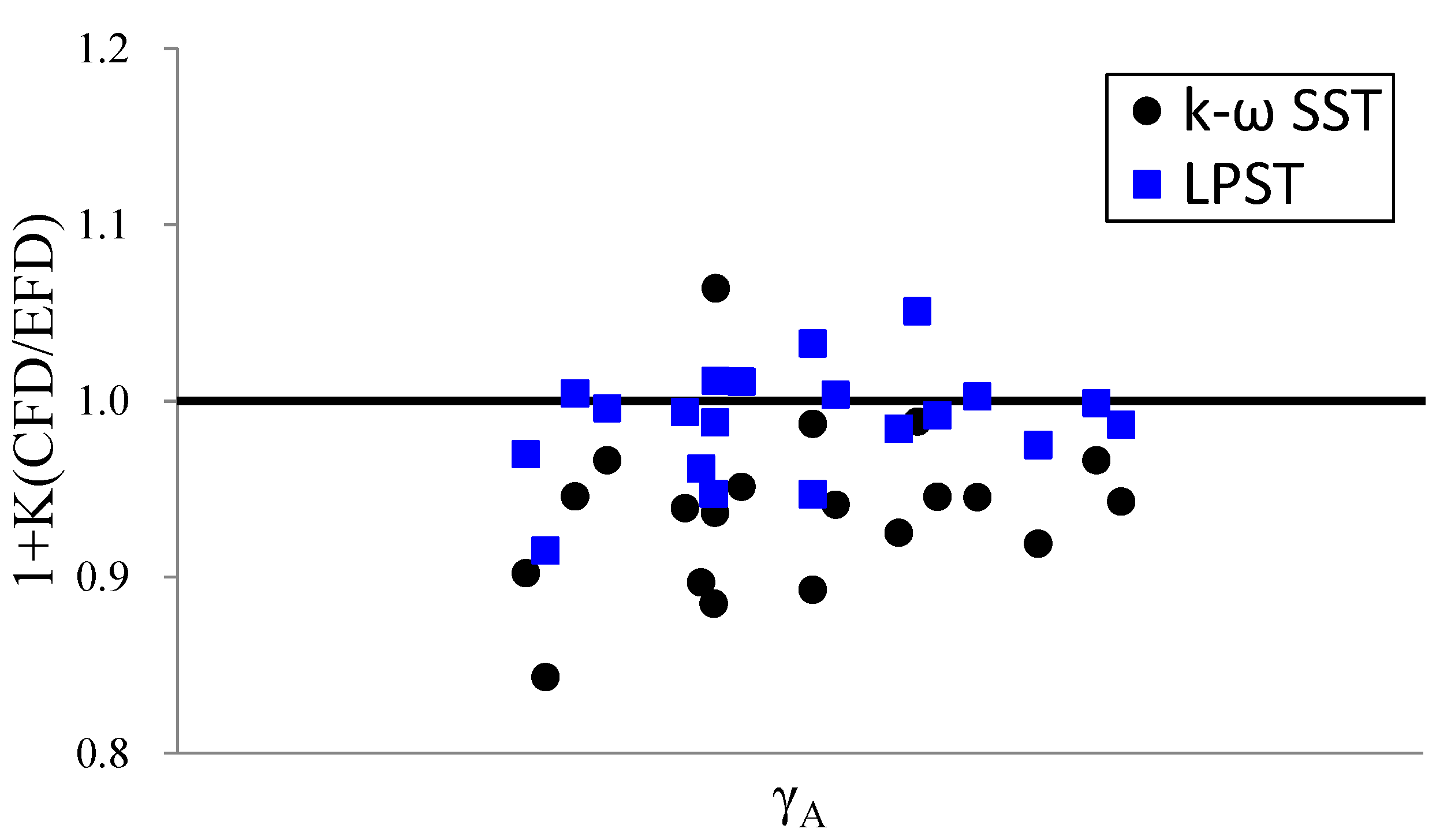
Considering the above, this paper confirms that the RSM has sufficient estimation accuracy of viscous resistance and wake distribution at the hull design stage. We calculated a JBC to compare the viscous resistance and wake distribution using k–omega SST and four RSM types. A JBC is a full-hull ship with a strong axial vortex. Therefore, it is suitable for evaluating the viscous resistance and wake distribution. The V&V is also calculated to study the grid dependency on the viscous resistance in this case. Furthermore, we compared the wake distribution of each RSM at the propeller plane. Finally, the best RSM was applied to 20 ships with various full and fine hull forms to calculate viscous resistance and compare it with the experimental results. For industrial use, this study could provide an important insight into the designing of various types of vessels.

2. Validation of Turbulence Models

To evaluate the ability of the RSM to estimate a ship’s flow, the uncertainty of the estimated viscous resistance due to turbulence modeling must be calculated using the V&V method. Fred Stern et al. [13] defined verification as the process of evaluating the numerical uncertainty, while validation is defined as the process of evaluating the model uncertainty. Herein, verification is performed using three types of a nonuniformly refined calculation grid, while validation is performed to evaluate the accuracy of $1+K$ using the benchmark experimental data.

2.1. Computational Conditions

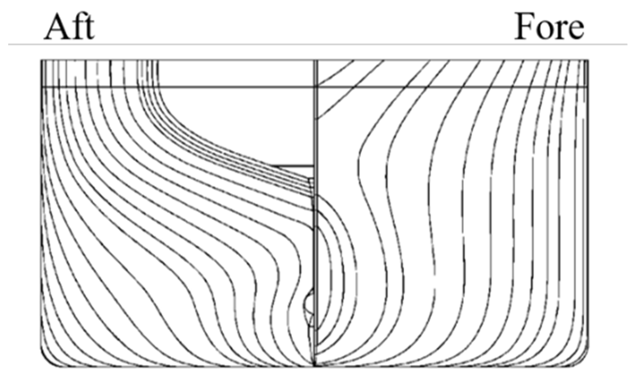
A JBC’s hull form was employed for validating the turbulence models. A JBC was designed by the National Maritime Research Institute (NMRI) in Japan. It was used to obtain CFD validation data, which were open to the public in the CFD Workshop 2015 held in Tokyo [5]. A JBC bodyplan is shown in Figure 1. The right side is the forepart, and the left side is the aft part. The principal dimensions of a JBC and the CFD calculations, which were performed on a model-scale ship, are shown in

Table 1. Principle dimensions of a JBC.

SHIP NAME		JBC
Model/Ship		Ship	Model
Length between perpendiculars	Lpp (m)	280.00	7.0000
Length on waterline	LDwl (m)	285.00	7.1250
Breath	B (m)	45.00	1.1250
Depth	D (m)	25.00	0.6250
Draft	d(m)	16.50	0.4125
Block coefficient	Cb	0.8580

.

The CFD calculations were performed using a STAR-CCM+ ver14.04, which is capable of solving the RANS equations of the k–omega SST model [14] and the RSM equation. The RSM variations, such as the LPS model, LPST model, QPS model, and elliptic blending (EB) model, were applied to investigate their ability to estimate the viscous resistance and wake distributions. The LPS model, which was proposed by Gibson and Launder [15], is the most basic RSM model employing a wall function. The LPST model was proposed by Rodi [16] that uses a model coefficient for the pressure-strain correlation term reported by Launder and Shima [17]. Generally, the LPST model provides more accurate calculations than the LPS model. In the QPS model, which was proposed by Speziale et al. [18], the high-order expansion of the pressure-strain correlation term is cut off. The EB model, which was proposed by Manceau and Hanjalić [19], is a low Reynolds–number model based on the formulation of the quasilinear QPS term near an inhomogeneous wall surface. An improved version of this model, which was proposed by Lardeau and Manceau [20], was implemented in the STAR-CCM+.

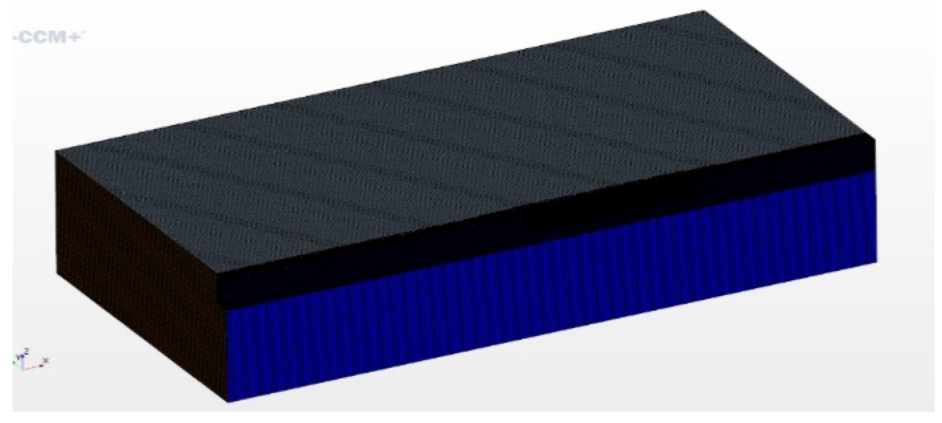
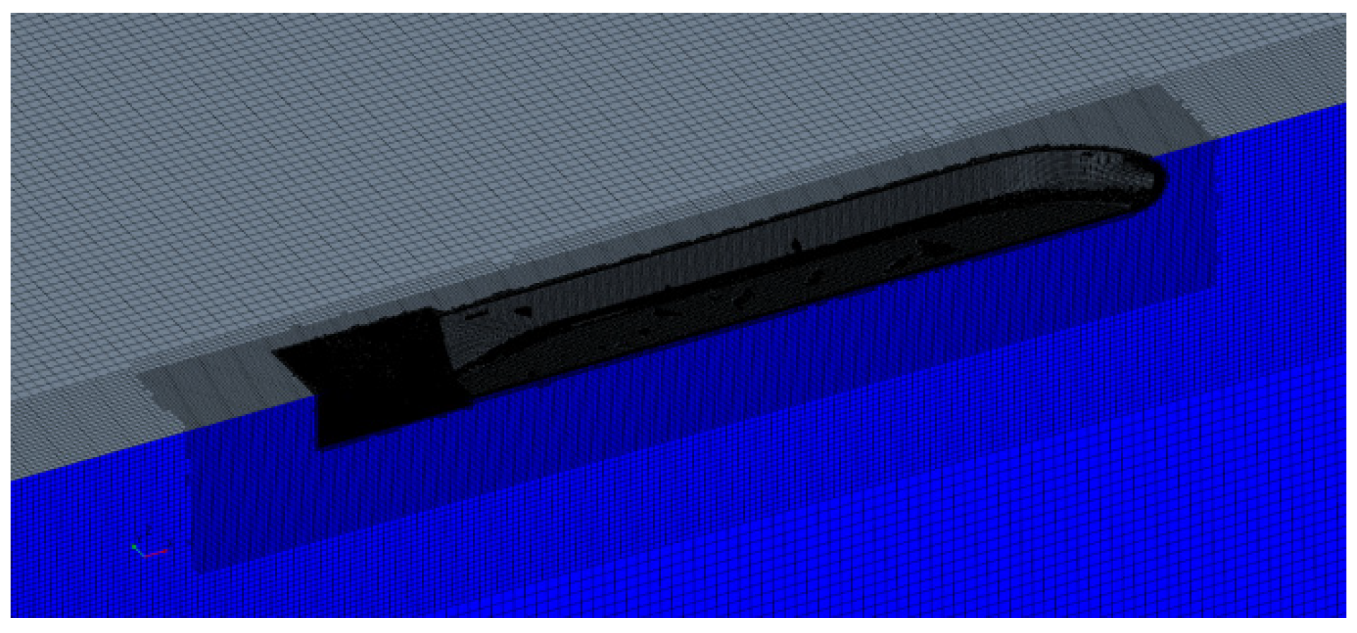
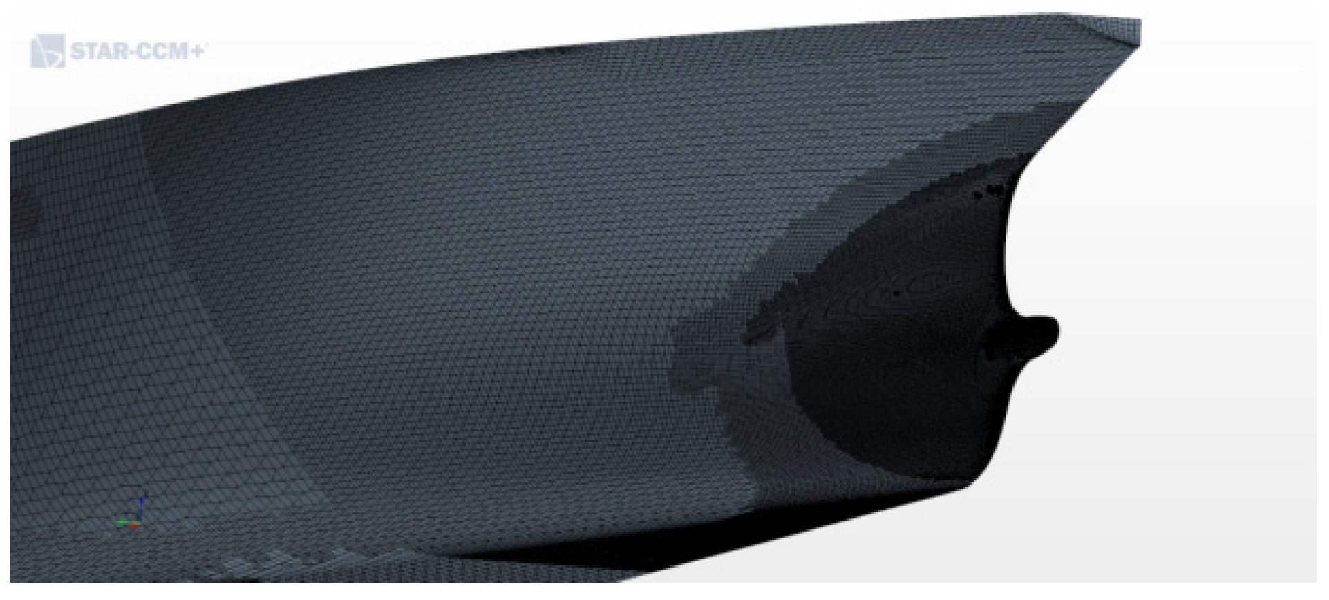
The computational domain has a length of 5.0 L_pp, a width of 2.5 L_pp, and a depth of 1.5 L_pp (Figure 2, Figure 3 and Figure 4). The upstream and side-boundary surfaces were set as the inlet, the downstream boundary surface was set as the outlet, and the slip condition was applied to ignore the wave effect at the top surface boundary. The computational cells were generated by a hexahedral element. The nondimensional distance (y+) from the hull surface to the first cell center was set to one (or less) for the low Reynolds–number model and to approximately 70 for the wall function turbulence model. The computational conditions are shown in

Table 2. Computational conditions.

Fn	0.142
Vm(m/s)	1.179
ρ(kg/m3)	998.7
ν × 10−6(m2/s)	1.0789
Rn	7.649 × 106

.

2.2. Verification and Validation (V&V) Method

The numerical and modeling uncertainties in the CFD simulation were evaluated on the basis of the ITTC procedures [21]. Verification, which assesses the numerical uncertainty in a simulation, was applied for estimating $1+K$ (K is the form factor), which is the standard measure of viscous resistance. Numerical errors generally include errors due to the number of iterations, time steps, and grid sizes. Herein, the time step is not considered because this calculation is a steady calculation, and hydrodynamic forces are calculated until convergence. Thus, only the numerical uncertainty $U_{SN}$ due to the grid size can be evaluated. 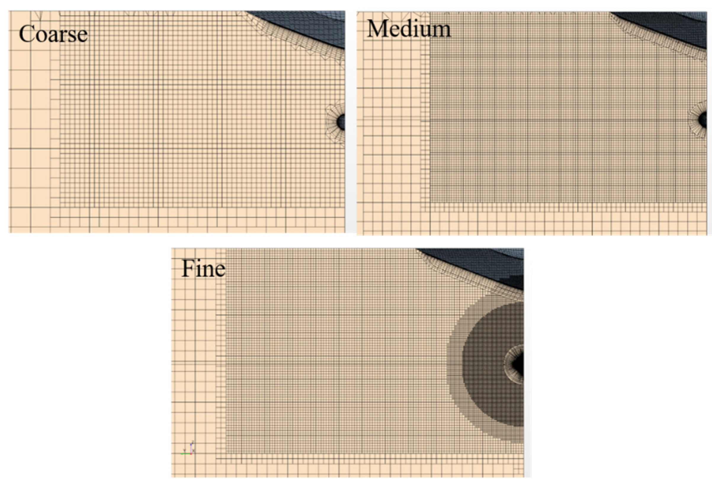$U_{SN}$ was evaluated by generating three types of grids with different sizes (coarse, medium, and fine). The number of cells in the coarse (NC3), medium (NC2), and fine (NC1) grids are shown in

Table 3. Results of grid refinement ratio $r_i$ .

		W.o.W.F.	W.F.
Fine	NC1	16,179,979	14,762,102
Midium	NC2	5,723,952	5,146,544
Coarse	NC3	1,728,686	1,475,687
	r	1.452	1.469
	r21	1.414	1.421
	r32	1.490	1.516

. The grid arrangements around the propeller plane for each grid type are shown in Figure 5. The definitions of the grid refinement ratios are shown in Equations (1) and (2).

$$r_{21}={\left(\frac{N_{C, 1}}{N_{C, 2}}\right)}^{1/3}$$

(1)

$$r_{32}={\left(\frac{N_{C, 2}}{N_{C, 3}}\right)}^{1/3}$$

(2)

The differences between the calculated $1+K$ in the medium–fine and coarse–medium grid solutions, as well as their ratio R, are defined as follows:

$${\epsilon }_{21}={\left(1+K\right)}_{medium}-{(1+K)}_{fine}$$

(3)

$${\epsilon }_{32}={(1+K)}_{coarse}-{\left(1+K\right)}_{medium}$$

(4)

$$R=\frac{{\epsilon }_{21}}{{\epsilon }_{ 32}}$$

(5)

The convergence patterns for grid refinement can be categorized into the following, depending on R:

(i)

Monotonic convergence: 0 < R < 1;

(ii)

Oscillatory convergence: R < 0;

(iii)

Divergence: R > 1.

In case (i) (monotonic convergence), to estimate the numerical errors caused by the cell size and evaluate the uncertainty of the form factor K, the generalized Richardson extrapolation (RE) was applied to the calculated results. The RE error can be calculated as follows:

$${\delta }_{RE}=\frac{{\epsilon }_{21}}{R^p-1}$$

(6)

$$p=\frac{ln\left(\frac{{\epsilon }_{32}}{{\epsilon }_{21}}\right)}{ln\left(r\right)}$$

(7)

where $p$ is the order of accuracy.

The numerical error in the fine grid calculation is defined as follows:

$${\delta }_{SN}=C{\delta }_{RE}=C\frac{{\epsilon }_{21}}{r^p-1}$$

(8)

The numerical uncertainty $U_{SN}$ evaluation is based on the correction factor $C$, which is calculated as follows:

$$C=\frac{r^p-1}{r^{p_{est}}-1}$$

(9)

Herein, a second-order upwind scheme was used; thus, $p_{est}=2$ in Equation (9). Therefore, the numerical uncertainty $U_{SN}$ can be calculated as follows:

$$U_{SN}=\left(\left|C\right|+\left|1-C\right|\right)\left|{\delta }_{RE}\right|$$

(10)

In case (ii) (oscillatory convergence), $U_{SN}$ can be calculated as follows:

$$U_{SN}=\left|\frac{1}{2}\left(S_U-S_L\right)\right|$$

(11)

where $S_U$ is the maximum $1+K$ in the grid convergence calculation and $S_L$ is the minimum $1+K$ in the grid convergence calculation.

In case (iii) (divergence), $U_{SN}$ cannot be estimated.

Validation is defined as the process of assessing the modeling uncertainty $U_{SN}$ using the benchmark experimental data. However, $U_{SM}$ cannot be calculated directly. However, the comparison error $E$ and the validation uncertainty $U_V$ can be calculated. Therefore, $E$ and $U_V$ are compared to evaluate $U_{SM}$.

The error $E$ is given by the difference in the validation data $D$ and ${(1+K)}_{fine}$ values as follows:

$$E=D-{(1+K)}_{fine}={\delta }_D-\left({\delta }_{SM}-{\delta }_{SN}\right)$$

(12)

where ${\delta }_D$ is the error in the validation experimental data, and ${\delta }_{SM}$ is the simulation modeling error. The validation uncertainty $U_V$ can be calculated as follows:

$$U_V{}^2=U_D{}^2+U_{SN}{}^2$$

(13)

If $\left|E\right|<U_V$, the combination of all the errors in $D$ and ${(1+K)}_{fine}$ is smaller than $U_V$, and validation is achieved at the $U_V$ level. If $U_V\ll \left|E\right|$ (the sign and magnitude of $E\approx {\delta }_{SM}$), the modeling needs to be improved.

2.3. Results of the Verification and Validation

The verification results for ${\epsilon }_{21}$, ${\epsilon }_{32}$, $R$, $p$, ${\delta }_{RE}$, $C$, ${\delta }_{fine}$, and $U_{SN}$ are shown in

Table 4. Results of the Verification.

	${\mathit{\epsilon }}_{21}$	${\mathit{\epsilon }}_{32}$	R	p	δRE	C	δfine(%(1 + K)fine)	USN(%(1 + K)fine)
k-ω SST	0.00091	0.13233	0.0068	13.361	6.236 × 10−6	130.910	0.07%	0.13%
k-ω SST w.W.F.	−0.00024	0.01456	−0.0166	-	-	-	-	0.55%
LPS	0.00165	0.01056	0.1560	4.835	3.045 × 10−4	4.678	0.11%	0.19%
LPST	0.00206	0.01126	0.1832	4.549	4.625 × 10−4	4.021	0.14%	0.25%
QPS	−0.00248	0.01076	−0.2303	-	-	-	-	0.32%
EB	0.00230	0.01086	0.2122	4.155	6.207 × 10−4	3.348	0.15%	0.26%

.

The calculated numerical uncertainty $U_{SN}$ (0.13%) of the k–omega SST model is lower than that obtained using the other turbulence models. Therefore, in the calculation of viscous resistance, the k–omega SST model without a wall function showed less grid dependency compared with the other turbulence models. The k–omega SST model with a wall function (wWF) is an oscillatory convergence ($R$ < 0). Thus, the uncertainty of the k–omega SST wWF model was calculated using method (ii) (oscillatory convergence) mentioned above. The RSM showed higher numerical uncertainty (approximately 0.25%) than the k–omega SST model; however, its uncertainty is generally lower than that obtained from the experiments. Nevertheless, the RSM results showed sufficiently low numerical uncertainty. The QPS model results in an oscillatory convergence ($R$ < 0). Thus, the uncertainty of the QPS model was calculated using method (ii) mentioned above.

The validation results are shown in

Table 5. Results of the validation for each turbulence model.

	E(%D)	UD(%D)	UV(%D)	EC(%D)
k-ω SST	4.65%	1.0%	1.01%	4.72%
k-ω SST w.W.F.	2.15%	1.0%	1.14%	-
LPS	−1.40%	1.0%	1.02%	−1.29%
LPST	−0.02%	1.0%	1.03%	0.13%
QPS	0.10%	1.0%	1.05%	-
EB	−6.57%	1.0%	1.04%	−6.41%

. $E$ is the comparison error defined in Equation (12) and $U_V$ is the validation uncertainty defined in Equation (13).

The validation results show that $E$ of the k–omega SST model is 4.72%, which is much larger than $U_V$ (1.01%). Therefore, the turbulence model needs to be improved. Meanwhile, the LPS model produces an overestimation of 1.29%. In particular, the LPST model produces an underestimation of 0.13%, which can be calculated with high accuracy. Moreover, the $E$ of the LPST model is much less than $U_V$ (1.03%). Therefore, the LPST model was close to the experimental results. The EB model produces an overestimation of 6.41%, which confirms that it is unsuitable for ship CFD calculations.

2.4. Validation of the Wake Distribution

The calculated wake distributions were compared with those obtained from stereoscopic particle image velocimetry (SPIV) measurements at 110 mm from the aft part. Here, we used the results obtained from SPIV measurements performed by NMRI [5].

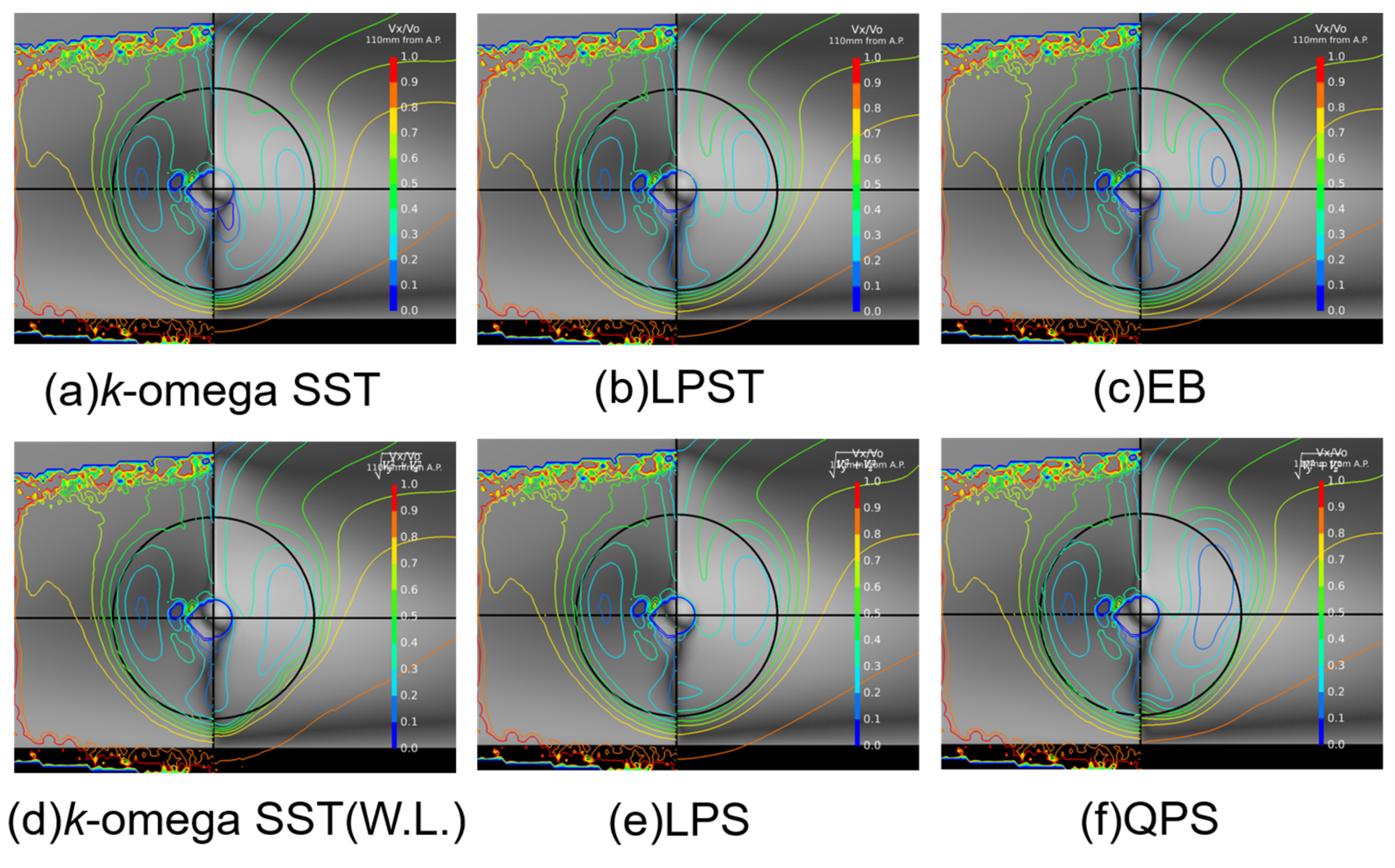
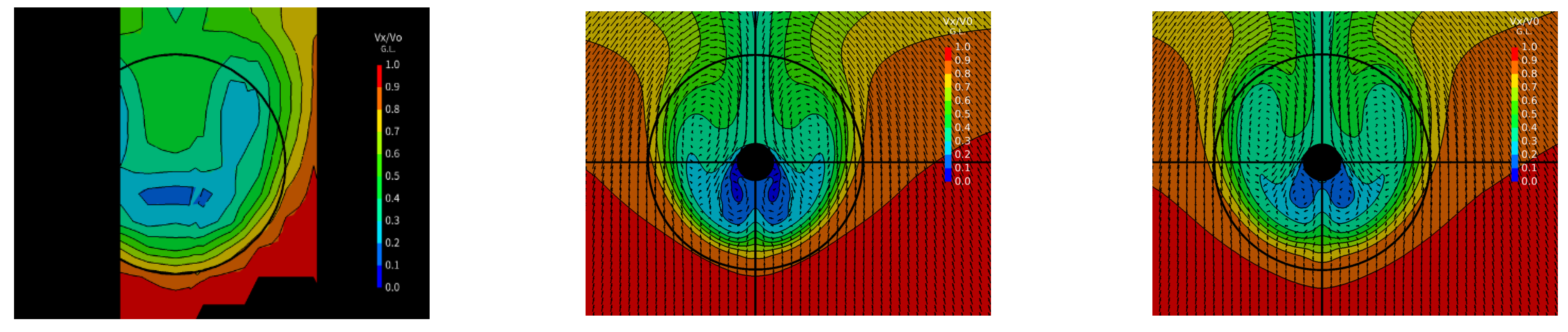
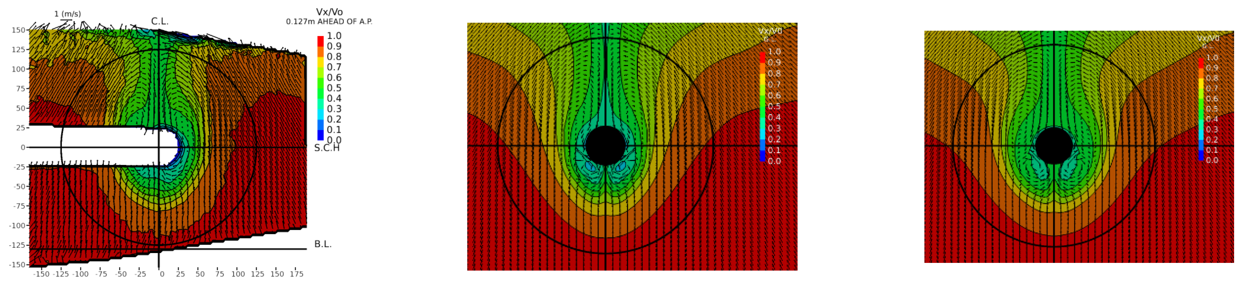
SPIV measurement results of the nondimensional longitudinal velocity at 110 mm from AP to bow side are shown in Figure 6, and the corresponding CFD calculation results are shown in Figure 7 (where $V_X$ is the longitudinal velocity (m/s) and $V_0$ is the ship speed (m/s)).

According to Figure 7, the calculated results obtained using the k–omega SST model are in good agreement with the SPIV measurement results. However, the contour at $V_X/V_0$ = 0.2 obtained using the k–omega SST model is different from the contour obtained from SPIV measurements. Furthermore, the contour obtained using the k–omega SST model has a small area at $V_X/V_0$ = 0.4 compared to the corresponding contour obtained from SPIV measurements. The shapes of contours at $V_X/V_0$ = 0.2 obtained using the LPS and LPST models are very close to those obtained from SPIV measurements. However, the longitudinal velocities at the propeller’s top position obtained using the LPS and LPST models are a little lower than those obtained from SPIV measurements. A contour at $V_X/V_0$ = 0.1 was obtained using the QPS and the EB models but no contour was obtained at $V_X/V_0$ = 0.1 from SPIV measurements. The calculated $V_X/V_0$ at the propeller plane obtained using the QPS model is smaller than that obtained from SPIV measurements, although not much smaller than that obtained using the LPS and LPST models. The overall shape of the wake obtained using the EB model is similar to that obtained from SPIV measurements.

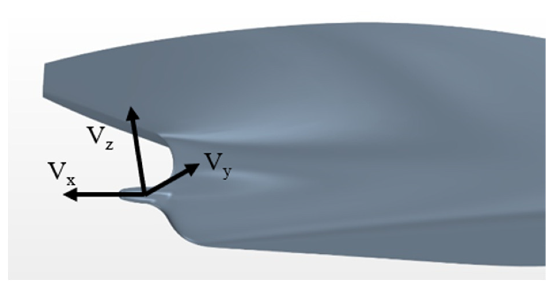
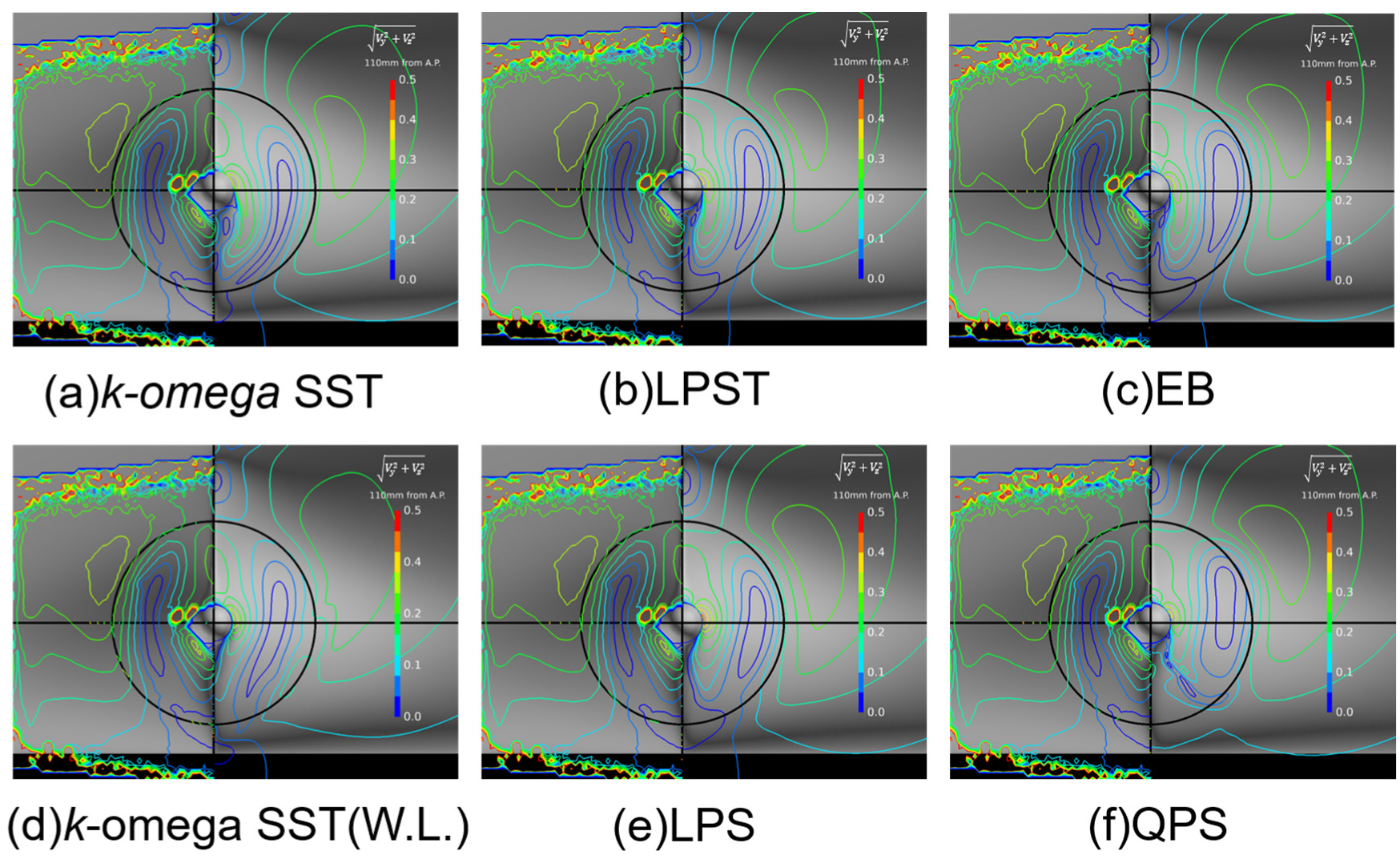
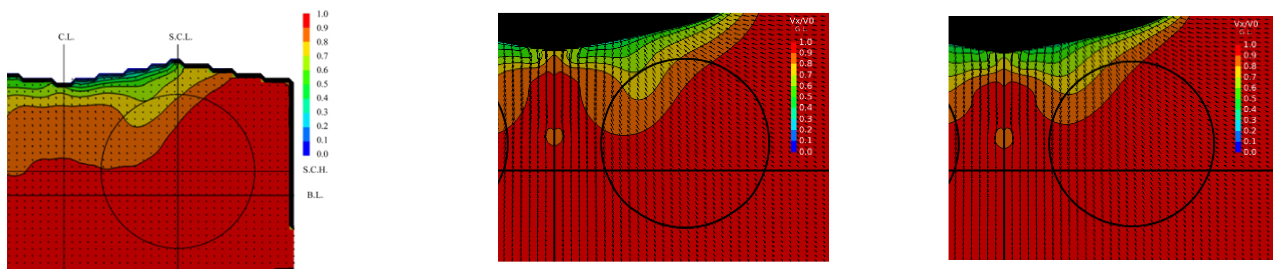
Figure 8 shows the magnitude distribution of the crossflow velocity obtained from CFD calculations at 110 mm from the AP to bow side and that obtained from SPIV measurements. The magnitude distribution of the crossflow velocity is useful for determining the longitudinal vortex intensity and core location. The crossflow velocity magnitude is defined as follows:

$$V_{cf}=\sqrt{V_y^2+V_z^2}$$

(14)

The contour at $V_{cf}=$ 0.05 obtained using the k–omega SST model is located lower than that obtained from SPIV measurements. Meanwhile, the $V_{cf}$ calculated using the LPS and LPST models is in good agreement with SPIV measurements. Using the LPS and LPST models, the longitudinal vortex intensity and core location can be calculated more accurately than those using the other turbulence models, such as the k–omega SST model. The $V_{cf}=$ 0.05 area calculated using the QPS and EB models is larger than that of the contour area calculated using the k–omega SST model. In relation to this, the QPS and EB models overestimated the wake and $1+K$.

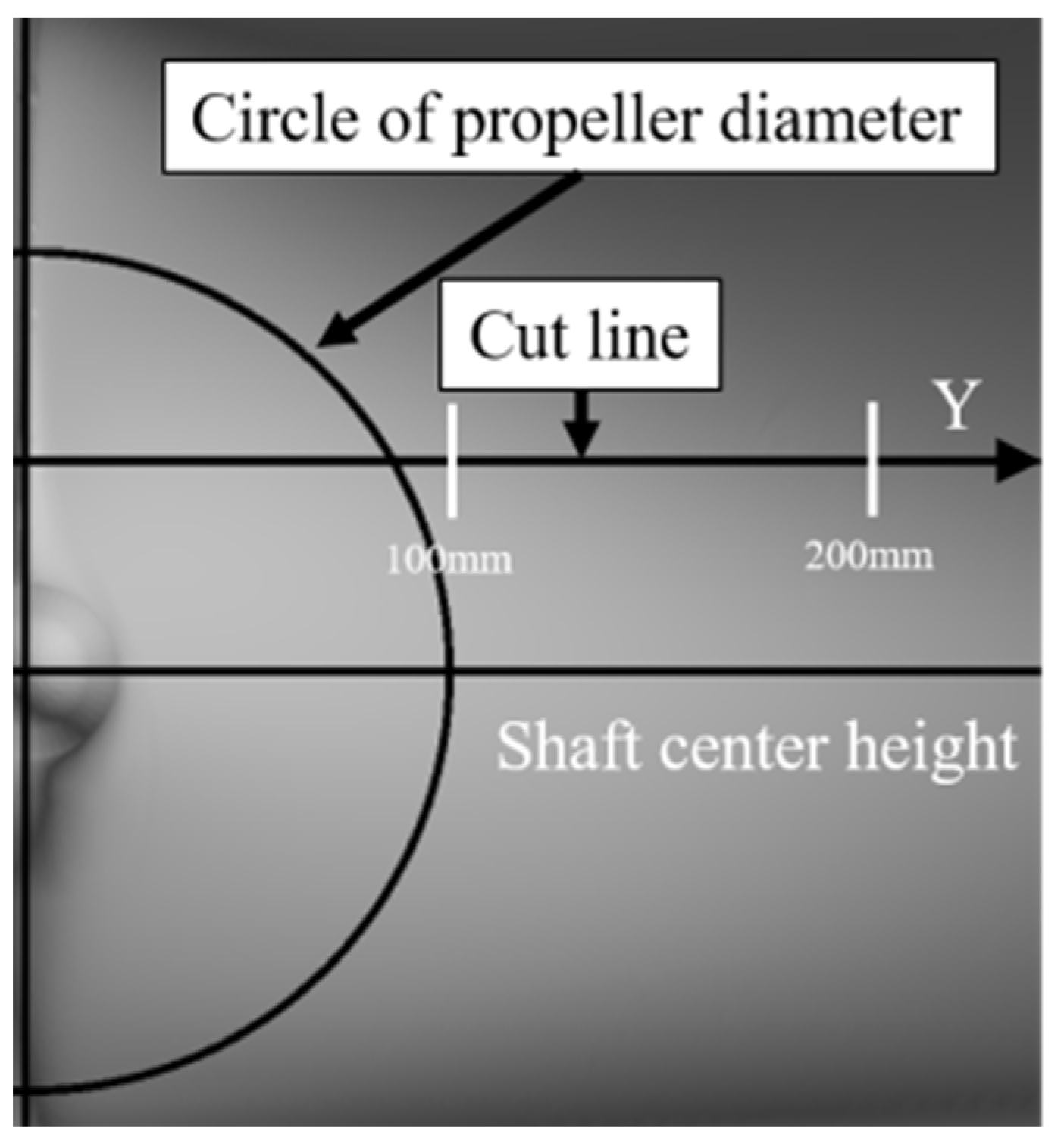
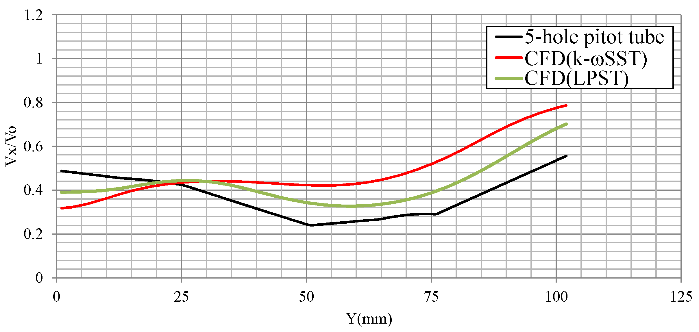
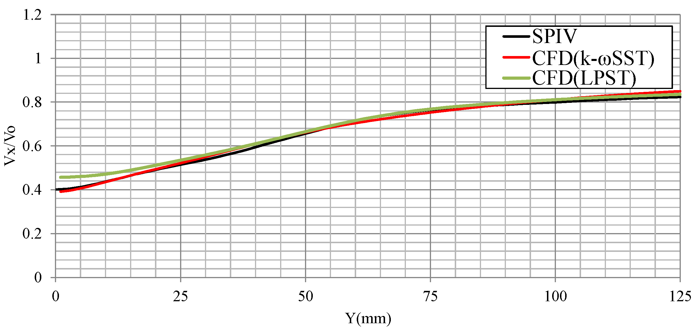
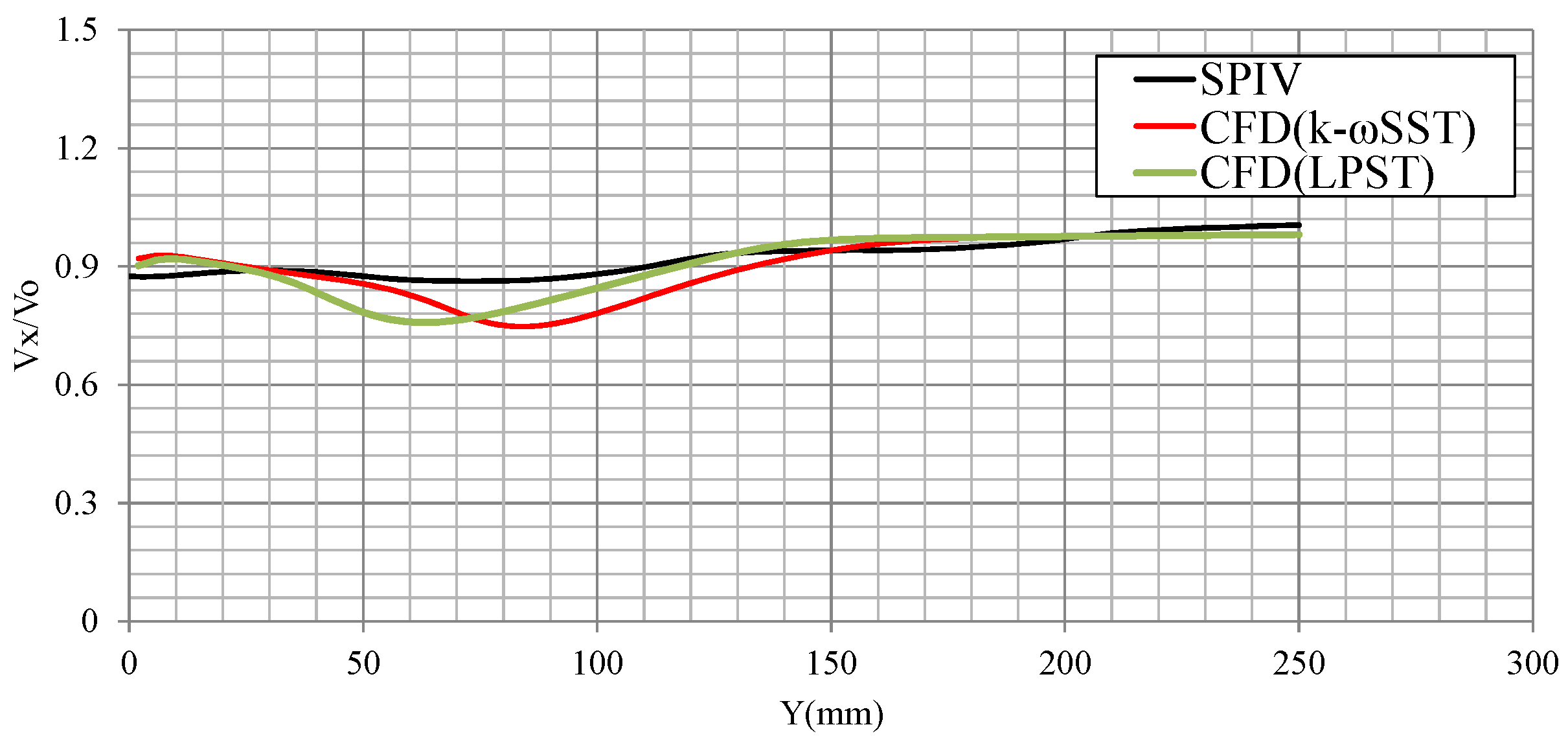
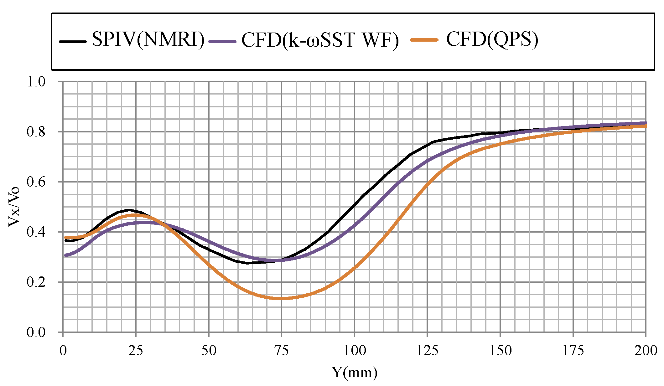
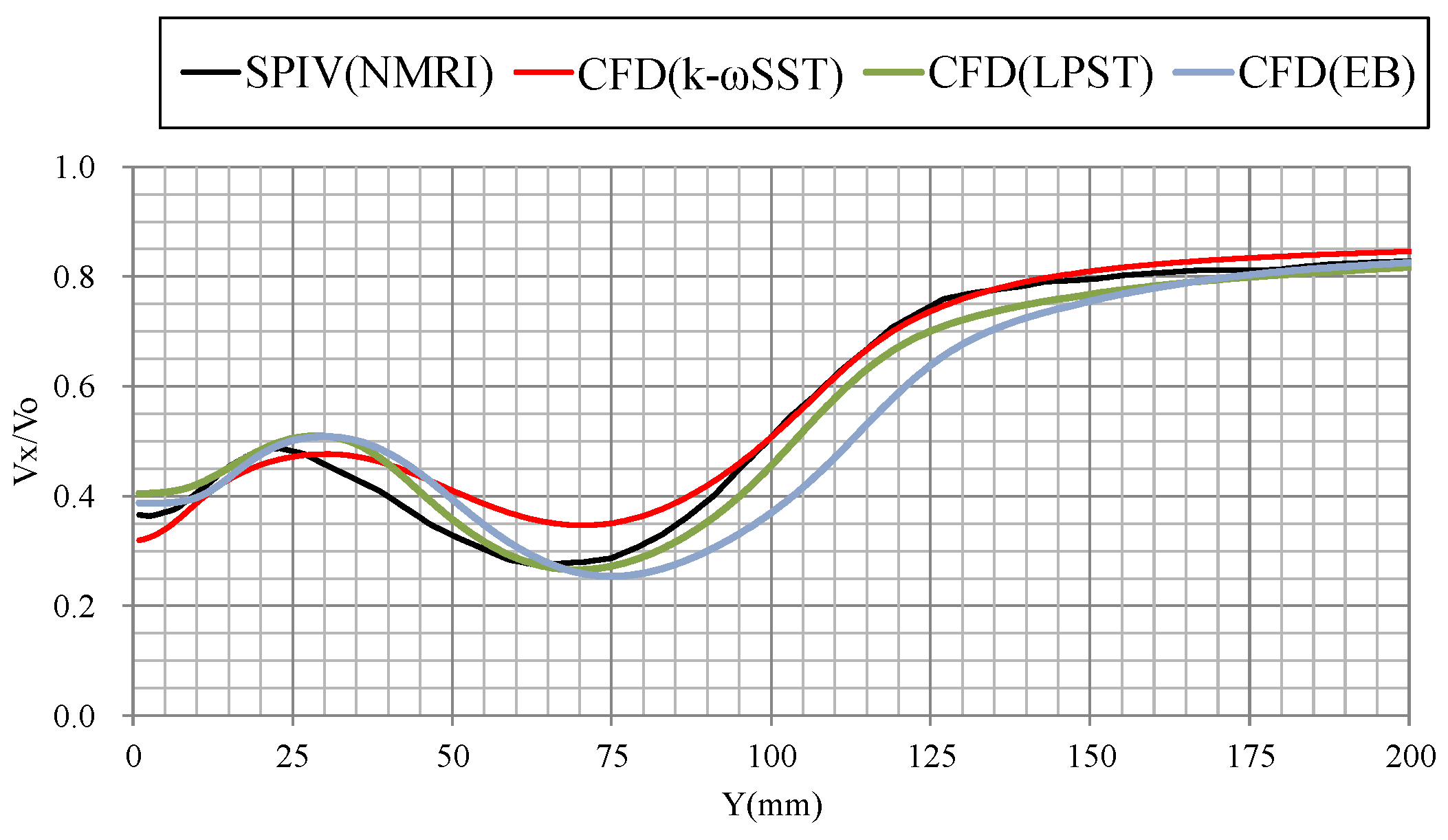
Figure 9 shows the definition and a schematic view of Y (mm). Figure 10 and Figure 11 show a comparison of the longitudinal velocity distribution along the horizontal line above the propeller shaft.

The k–omega SST wWF model (Figure 10) also showed good agreement around Y = 75 mm. However, the k–omega SST wWF model showed a large difference between 100 mm and 150 mm. Although the EB model (Figure 11) was capable of estimating the stern longitudinal vortex strength with high accuracy, it is considered that the hydrodynamic force was overestimated because the wake is generally large. As shown in Figure 11, the LPST model can estimate a wake around Y = 75 mm with high accuracy. If the vortex core can be accurately estimated, it will be possible to design a wake-adapted propeller with high accuracy.

The V&V analysis of $1+K$ presented in Section 2.3 indicates that the k–omega SST model showed lower numerical uncertainty and higher model uncertainty compared to the RSM. The k–omega SST model is considered an isotropic eddy viscosity model. Therefore, the appropriate turbulence model needs to be shifted from the k–omega SST model to the RSM.

3. Validation of the Calculation Results of the k–Omega SST Model and the RSM, Depending on the Ship Type

In Section 2, the numerical and model uncertainties in the calculation of the viscous resistance of a JBC using the k–omega SST model and the RSM were evaluated. It was also confirmed that the LPST model is capable of estimating the viscous resistance with the highest accuracy in our setting. However, it is important to evaluate whether the LPST model is suitable for accurate calculations not only for a JBC, such as a full hull–form ship but also for fine hull–form ships with a weak stern longitudinal vortex.

In this section, we demonstrated the ability of the LPST model to estimate the viscous resistance $1+K$ with higher accuracy than the k–omega SST model for various hull form types. For this purpose, the LPST model was applied to twenty ships with various full and fine hull forms to calculate $1+K$ and compare it with the experimental results.

3.1. Ship Types Used in the Calculations

Twenty different ships with a wide range of ${\gamma }_A$ and L_pp/B were examined. ${\gamma }_A$ is defined in Equation (15) as follows:

$${\gamma }_A=\frac{B/L}{1.3\left(1-C_b\right)-0.031l_{cb}}$$

(15)

where ${\gamma }_A$ is the run coefficient, B is the width, $C_b$ is the block coefficient, and $l_{cb}$ is the center of buoyancy (%L_pp).

Figure 12 shows twenty ships of different ${\gamma }_A$ and L_pp/B, including a JBC model, a KVLCC2 model [22], a KRISO container ship (KCS) model [22], and model 5415 [22], which are open to the public. The other ship types are general commercial ships, such as bulk carriers, gas carriers, car carriers, and training ships. These ships are original vessels that have not been opened. Therefore, the range of ${\gamma }_A$ is not possible to disclose details.

Table 6. List of the calculation conditions of the objective ships.

No.	Name	Rn
1	Ship A	9.79 × 106
2	Ship B	7.93 × 106
3	Model5415	5.72 × 106
4	Ship C	4.37 × 106
5	Ship E	7.13 × 106
6	JBC	6.73 × 106
7	Ship F	7.86 × 106
8	Ship G	8.80 × 106
9	Ship H	8.70 × 106
10	Ship I	7.45 × 106
11	Ship J	1.04 × 106
12	Ship K	8.31 × 106
13	Ship L	1.15 × 107
14	Ship M	7.66 × 106
15	Ship N	8.98 × 106
16	KCS	1.30 × 107
17	KVLCC	6.37 × 106
18	Ship O	6.68 × 106
19	Ship P	7.37 × 106
20	Ship Q	7.28 × 106

shows list of the calculation conditions of the objective ships.

3.2. Result of the CFD Calculation

Figure 10 shows $1+K$, which was calculated from the hydrodynamic force using the method described in Section 2. It is expressed as the ratio of the experimental value to the calculated value. The horizontal axis indicates the run coefficient because it is known to have a strong correlation with $1+K$. The black circles show the results obtained using the k–omega SST model, whereas the blue squares show the results obtained using the LPST model. For the friction line calculation, the Schoenherr formula described in Equation (16) was used. Model 5415 was excluded since it was difficult to determine its $1+K$ value.

$$C_{f0}=\frac{0.463}{{\left({\log }_{10}Rn\right)}^{2.6}}$$

(16)

Standard errors (SE) were compared to quantitatively evaluate the accuracy of the turbulence model. The formulas of the SE in (17) and (18) were used.

$$SD=\sqrt{\frac{{\displaystyle \sum {\left(X_i-\overline{X}\right)}^2}}{\left(N-1\right)}}$$

(17)

$$SE=\frac{SD}{\sqrt{N}}$$

(18)

where $C_{f0}$ is the friction coefficient and $Rn$ is the Reynolds number.

The SEs were compared to quantitatively evaluate the accuracy of the turbulence model. They were calculated using Equation (18).

Figure 13 shows the $1+K$ ratio of CFD and EFD of k–omega SST and LPST.

As shown in Figure 10, the LPST model produces a value much closer to 1.0 than the k–omega SST. The SE of the k–omega SST model was 0.023. Meanwhile, the SE of the LPST model was 0.010. It is confirmed that the LPST model is capable of estimating the viscous resistance ($1+K$) with higher accuracy than that of the k–omega SST model for various hull form types in our setting. Specifically, it achieves high accuracy for large ${\gamma }_A$ values.

Figure 14, Figure 15, Figure 16, Figure 17, Figure 18 and Figure 19 show a comparison of the wake distribution obtained using EFD and CFD calculations. Figure 17, Figure 18 and Figure 19 show a comparison of the longitudinal velocity distribution along the horizontal line above the propeller shaft. Here, the EFD data of the KVLCC2 model were obtained from a wind tunnel test [23]. The KCS model and model 5415 results were obtained from SPIV measurements conducted in Akishima Laboratories (Mitsui Zosen) Inc., Tokyo, Japan. Moreover, the CFD calculations were performed using the Rn values used in the experiments.

Figure 14 shows a comparison of the wake distribution obtained using the KVLCC2 model. The hull form shown is that of a full ship similar to a JBC. A stern longitudinal vortex can be observed. Figure 15 shows a comparison of the wake distribution obtained using the KCS model. The KCS model is that of a fine hull–form ship (i.e., a container ship). No stern longitudinal vortex hooks were obtained using this model. Figure 16 shows a comparison of the wake distribution obtained using model 5415. A buttock-flow profile can be observed. The calculation results obtained using the KVLCC2 model shows the same trend as those obtained using a JBC model, as shown in Figure 14. The contour at $V_X/V_0$ = 0.4 obtained using the k–omega SST model had a different shape from that obtained from SPIV measurements. Meanwhile, the shape of the contour at $V_X/V_0$ = 0.4 obtained using the LPST model was very similar to that obtained from the EFD calculation results. The calculation results obtained using the KCS model are shown in Figure 15 and Figure 18. There was almost no difference between the results produced by the k–omega SST and the LPST models. It is confirmed that the k–omega SST model is capable of sufficiently estimating the wake distribution of fine hull forms. The same trend is observed in the results produced by model 5415, as shown in Figure 16 and Figure 19.

4. Conclusions

Herein, we carried out a resistance calculation for a JBC to compare the viscous resistance and wake distribution using k–omega SST and four types of RSMs. The V&V was also calculated to study the grid dependency of the viscous resistance. Consequently, we were able to show the difference in viscous resistance of each RSM and confirmed that LPS and LPST are appropriate for ship CFD calculations in our setting. The comparisons show that the RSM accurately predicts most of the experimentally observed flow features in the stern and near-wake regions, whereas the two-equation model predicts only the overall qualitative trends. The LPST model was applied to twenty ships with various full and fine hull forms to calculate $1+K$ and compare it with the experimental results. The calculation results confirmed that LPST has a high accuracy of viscous resistance not only for full ships but also for fine-hull forms in our setting. A summary of details is as follows:

• The calculated numerical uncertainty $U_{SN}$ of the k–omega SST model without a wall function is lower than that of the other turbulence models. Therefore, the k–omega SST model without a wall function shows less grid dependency in the calculation of viscous resistance compared with the other turbulence models.
• The RSM shows a numerical uncertainty (approximately 0.25%) higher than that of the k–omega SST model. However, its uncertainty is generally smaller than that obtained from experiments. Nevertheless, the RSM is a promising turbulence model with low numerical uncertainty.
• The comparison error $E$ of the k–omega SST model is much larger than the validation uncertainty $U_V$. Therefore, the turbulence model needs to be improved. Meanwhile, the $E$ of the LPS and LPST models is much less than $U_V$. Thus, this turbulence model is accurate since it produces results similar to those obtained from experiments.
• The calculated wake distributions using RSMs exhibit good agreement with SPIV measurements, except for the QPS model. Specifically, using the LPS and LPST models, the size of the stern longitudinal vortex and the wake distribution under the shaft can be estimated with high accuracy.
• The LPST model is capable of estimating the axial velocity distribution along the horizontal line above the propeller shaft with high accuracy. If the vortex core can be estimated accurately, it will be possible to design a wake-adapted propeller with high accuracy.
• The LPST shows a small difference between the EFD and CFD calculations. The standard error SE of the LPST model is smaller than the SE of the k–omega SST model. Therefore, the LPST model is capable of estimating the viscous resistance with high accuracy in our setting.
• The calculation results obtained using the KVLCC2 model show the same trend as those of a JBC hull form. Moreover, it is clear that the LPST model is capable of accurately estimating the stern longitudinal vortex hooks.
• The calculation results of the KCS and Model 5415 show that there is almost no difference from those produced by the k–omega SST and LPST models. Therefore, it was confirmed that the k–omega SST model is capable of efficiently estimating the $1+K$ and wake distribution of fine hull–forms.

We evaluated the comparison error to confirm the superiority of the LPST for model-scale calculation. Herein, the effects of the turbulence models were evaluated using V&V. From an engineering viewpoint, this is critical in ship design. The RSM is the most promising turbulence model of the LPST models for RANS CFD calculations in our setting. For industrial use, this study could provide important insights into the designing of various types of vessels.

References

1. IMO, MEPC. Guide Lines on Survey and Certificaion of the Energy Efficiency Design Index (EEDI). MEPC 63/23/Add.1 Annex 10. 2012. Available online: https://wwwcdn.imo.org/localresources/en/OurWork/Environment/Documents/214(63).pdf (accessed on 1 February 2020).
2. IMO, MEPC. Initial Imo Strategy on Reduction of Ghg Emissions From Ships. MEPC 72/17/Add.1 Annex 11. 2018. Available online: https://wwwcdn.imo.org/localresources/en/OurWork/Environment/Documents/ResolutionMEPC.304(72)_E.pdf (accessed on 1 February 2020).
3. Su, Y.; Lin, J.; Zhao, D.; Guo, C.; Guo, H. Influence of a pre-swirl stator and rudder bulb system on the propulsion performance of a large-scale ship model. Ocean Eng. 2020, 218, 108189. [Google Scholar] [CrossRef]
4. Pena, B.; Luofeng, H. A review on the turbulence modelling strategy for ship hydrodynamic simulations. Ocean Eng. 2021, 241, 110082. [Google Scholar] [CrossRef]
5. Webpage, Tokyo 2015 a Workshop on CFD in Ship Hydrodynamics. 2015. NMRI. Available online: http://www.t2015.nmri.go.jp/index.html (accessed on 1 February 2020).
6. Terziev, M.; Tezdogan, T.; Incecik, A. Application of Eddy-Viscosity Turbulence Models to Problems in Ship Hydrodynamics. In Ships and Offshore Structures; Taylor & Francis: Oxfordshire, UK, 2020; Volume 15. [Google Scholar]
7. Visonneau, M.; Deng, G.; Queutey, P.; Guilmineau, E.; del Toro Llorens, A. High-Fidelity Computational Analysis of an Energy-Saving Device at Model-scale. In Proceedings of the Hull Performance & Insight Conference (HullPIC), Turin, Italy, 13–15 April 2016. [Google Scholar]
8. Gaggero, S.; Villa, D.; Viviani, M. An extensive analysis of numerical ship self-propulsion prediction via a coupled BEM/RANS approach. Appl. Ocean Res. 2017, 66, 55–78. [Google Scholar] [CrossRef]
9. Andrea, F.; Nastia, D.; Ivana, M.; Roko, D. Numerical and experimental assessment of nominal wake for a bulk carrier. J. Mar. Sci. Technol. 2019, 24, 1092–1104. [Google Scholar]
10. Tatsuo, N.; Yoshinobu, Y.; Masaru, S.; Chisachi, K. Application of Fully-resolved Large Eddy Simulation to KVLCC2 –Bare Hull Double Model at Model Ship Reynolds Number. J. Jpn. Soc. Nav. Archit. Ocean. Eng. 2012, 16, 1–9. [Google Scholar]
11. Kornev, N.; Abbas, N. Vorticity structures and turbulence in the wake of full block ships. J. Mar. Sci. Technol. 2018, 23, 567–579. [Google Scholar] [CrossRef]
12. Liefvendahl, M.; Johansson, M. Wall-modeled LES for ship hydrodynamics in model-scale. J. Ship Res. 2021, 65, 41–54. [Google Scholar] [CrossRef]
13. Stern, F.; Wilson, R.V.; Coleman, H.W.; Paterson, E.G. Verification and Validation of CFD Simulations; IIHR Report No. 407; Iowa Institute of Hydraulic Research College of Engineering, The University of Iowa: Iowa City, IA, USA, 1999. [Google Scholar]
14. Menter, F.R. Two-Equation Eddy-Viscosity Turbulence Models for Engineering Applications. AIAA J. 1994, 32, 1598–1605. [Google Scholar] [CrossRef] [Green Version]
15. Gibson, M.M.; Launder, B.E. Ground effects on pressure fluctuations in the atmospheric boundary layer. J. Fluid Mech. 1978, 86, 491–511. [Google Scholar] [CrossRef]
16. Rodi, W. Experience with Two-Layer Models Combining the k-e Model with a One-Equation Model Near the Wall. In Proceedings of the 29th Aerospace Sciences Meeting, AIAA 91-0216, Reno, NV, USA, 7–10 January 1991. [Google Scholar]
17. Launder, B.E.; Shima, N. Second Moment Closure for the Near-Wall Sublayer. Dev. Appl. AIAA J. 1989, 27, 1319–1325. [Google Scholar] [CrossRef]
18. Speziale, C.G.; Sarkar, S.; Gatski, T.B. Modelling the pressure-strain correlation of turbulence: An invariant dynamical systems approach. J. Fluid Mech. 1991, 227, 245–272. [Google Scholar] [CrossRef]
19. Manceau, R.; Hanjalic, K. Elliptic blending model: A new near-wall Reynolds-stress turbulence closure. Phys. Fluids 2002, 14, 744–764. [Google Scholar] [CrossRef]
20. Lardeau, S.; Manceau, R. Computations of Complex Flow Configurations Using a Modified Elliptic-Blending Reynolds-Stress Model. In Proceedings of the 10th Engineering Turbulence Modelling and Experiments, Modelling and Measurement Conference, Marbella, Spain, 17–19 September 2014. [Google Scholar]
21. ITTC. ITTC Recommended Procedures and Guidelines—Uncertainty Analysis in CFD Verification and Validation Methodology and Procedures., Approved 28th ITTC 2017, 09/2017. Available online: https://www.ittc.info/media/8153/75-03-01-01.pdf (accessed on 1 February 2020).
22. Webpage, SIMMAN 2008. Available online: http://www.simman2008.dk/ (accessed on 1 February 2020).
23. Lee, S.-J.; Kim, H.-R.; Kim, W.-J.; Van, S.-H. Wind tunnel tests on flow characteristics of the KRISO 3600 TEU containership and 300K VLCC double-deck ship models. J. Ship Res. 2003, 47, 24–38. [Google Scholar] [CrossRef]
Figure 1. Bodyplan of a JBC.
Jmse 10 00777 g001
Figure 2. Volume grid of whole area.
Jmse 10 00777 g002
Figure 3. Volume grid of JBC around the hull.
Jmse 10 00777 g003
Figure 4. Surface grid of JBC around the stern.
Jmse 10 00777 g004
Figure 5. Grid arrangement around the propeller plane.
Jmse 10 00777 g005
Figure 6. Coordinate system of the CFD calculation.
Jmse 10 00777 g006
Figure 7. Distribution of longitudinal velocity of SPIV (Left) and CFD (Right) at 110 mm from AP to bow side. (a) k–omega SST (b) LPST (c) EB (d) k–omega SST (W.L.) (e) LPS (f) QPS.
Jmse 10 00777 g007
Figure 8. Crossflow distribution of SPIV (Left) and CFD (Right) at 110 mm from AP to bow side. (a) k–omega SST (b) LPST (c) EB (d) k–omega SST (W.L.) (e) LPS (f) QPS.
Jmse 10 00777 g008
Figure 9. Schematic view of a cut line.
Jmse 10 00777 g009
Figure 10. Longitudinal velocity distribution along the horizontal line above the propeller shaft calculated by wall function models.
Jmse 10 00777 g010
Figure 11. Longitudinal velocity distribution along the horizontal line above the propeller shaft calculated by low Reynolds number models.
Jmse 10 00777 g011
Figure 12. γ A and Lpp/B of types of ships.
Jmse 10 00777 g012
Figure 13. Result of CFD calculation ( 1 + K ).
Jmse 10 00777 g013
Figure 14. Comparison of results of the wake distribution of KVLCC2. ((Left): EFD, (Center): k-omega SST, (Right): LPST).
Jmse 10 00777 g014
Figure 15. Comparison of results of the wake distribution of KCS. ((Left): EFD, (Center): k-omega SST, (Right): LPST).
Jmse 10 00777 g015
Figure 16. Comparison of results of the wake distribution of Model5415. ((Left): EFD, (Center): k-omega SST, (Right): LPST).
Jmse 10 00777 g016
Figure 17. Axial velocity distribution of KVLCC2 along the horizontal line above propeller shaft.
Jmse 10 00777 g017
Figure 18. Axial velocity distribution of KCS along the horizontal line above propeller shaft.
Jmse 10 00777 g018
Figure 19. Axial velocity distribution of Model5415 along the horizontal line above propeller shaft.
Jmse 10 00777 g019