CFD Method to Study Hydrodynamics Forces Acting on Ship Navigating in Confined Curved Channels with Current

Abstract

The bending section of the restricted channel is one of the most accident-prone areas for inland ships, but few clear investigations on the curvature effect have been conducted till now. Therefore, this paper presents numerical research of the curvature effect in confined bending channels on ship hydrodynamics. The unsteady Navier–Stokes equations closed by the realizable K-Epsilon turbulence model are utilized to simulate the flow around a three-dimensional inland ship. A mesh verification analysis is performed to select the most suitable grid size, and the CFD model is validated in a regular confined channel by comparing the numerical resistance forces with those from experiments. The impacts of the channel slope angle, channel radius, ship type (ship length), and current velocity in curved channels on ship hydrodynamics are studied with their influence patterns and mechanisms being analyzed in detail. Results show that channel radius only affects the yaw moment much, whereas ship hydrodynamics are greatly sensitive to the slope angle only when the angle is below a certain threshold value. Compared with short ships, much stronger spiral currents can be noticed passing through long ships in the same channel configuration. Current velocity affects both resistance and yaw moment a lot, with a critical current velocity for sway force.

1. Introduction

The inland waterway transport has a range of advantages over rail and road transport including large capacity, low cost, and low energy consumption, etc. There are various forms in inland rivers or canals, such as bending, straight, and bifurcated sectors, among which the bending sectors are the most common and dangerous zones. Many scholars were devoted to figuring out the flow characteristics in bending zones [1,2,3,4], and the general flow characteristics of the water in the bend have been understood. The current will move in a curve when it flows through the bending zones due to the centrifugal force, causing unequal water levels between both banks [5,6]. The water surface is not perpendicular to the gravity direction of the ship, which affects the stability of the ship during cornering. The surface current tends to own higher velocity and centrifugal force, flowing towards the concave bank; whereas, the opposite is true for the bottom current as it flows to the convex bank due to the low velocity and centrifugal force. Eventually, a circulation current is formed coupled with the gravitational force and frictional resistance of the flow [7,8,9]. What’s more, this further causes uneven distribution of water depths between both banks. The complex flow characteristics is the root cause for the high accidental rate for ships’ passing the bending zones, due to which the motion state of ships will be consequently changed, bringing enormous difficulty in ships’ maneuvering.

Importantly, when ships sail in shallow bending zones, the flow characteristics in such regions will also change accordingly, which makes it different from what it would be without ships navigating. In recent years, some research related to ship navigation in curved channels has been conducted. Combining experiments, Maslikova et al. [10] proposed a model to describe the joint effect of a flow on curved banks, including in the process of rock thawing, and the impact of ship waves. Vujičić et al. [11] gave a practical and theoretical approach to assessing safe navigating in waterways based on expertise and experience, the aim of which is to propose a way of control for seamen working at sea. The works of Ai et al. [12,13] both firstly analyzed the factors influencing the occurrence of accidents in curved channels, and then [12] brought forward mathematical modeling of navigational reliability of curved channels to assess the safe navigation probability, Ref. [13] estimated ship passing capacity, the minimum distance between bridge pier surface, and channel edge. Afterwards, Ai and Zhu [14] came up with the drift angle calculation equation and found that a ship’s navigation drift angle is strictly linked to a range of parameters including channel’s radius, water depth, and ship’s draft, and so on. Based on the ship model test results for the lower reaches of the Hanjiang River MaKou reach, Wang and Cheng [15] summed up the relationship between channel width and flow, indicating that, at about the same speed, the navigation width of sailing through the bend upward is substantially lower than the navigation width of sailing through the bend below. Yang et al. [16] studied the influence brought by a series of key parameters (channel angle, h/T ratio, ship speed, etc.) in confined curved fairways on ship hydrodynamics via CFD technique, which helps to understand the flow behaviour around an inland ship in such sensitive waters.

Nevertheless, most researchers are numerically concerned with the water flows in the bends without ships sailing. Few numerical investigations have looked at the details of the flow field in curves with ships sailing so far. Therefore, it is essential to research the effect of various bending configurations and currents on ship hydrodynamics in confined curved fairways.

Nowadays, the CFD technique has witnessed great progress and it has been adopted as a greatly effective tool to conduct explorations by researchers in both deep waters and confined shallow waters due to its advantages of low cost, short cycle time, and high accuracy. Seemontini Roy Choudhury et al. [17] researched steady motions of drift and yaw based on a specific crude ship with the CFD solver SHIPFLOW both in deep and shallow waters, and the simulation results were in agreement with those from experiments. Using STARCCM+, Jonas Bechthold and Marko Kastens [18] simulated the sinking and trimming of three Postpanmax container ships in confined shallow waters. Their results showed good consistency with model test. Additionally, Ivan Shevchuk and Nikolai Kornev [19] assessed the effect of shallow water conditions on ship hull vibration hydrodynamic exciters with the CFD tool OpenFOAM, through which it is found that the ship’s stern may be affected by intermittent pressures and moments due to the depth limit.

Lu Zou et al. [20] utilized CFD methods to study the bank effects on a tanker hull by considering varying water depths, ship-to-bank distances, and bank geometries, and conducted verification and validation by a grid convergence survey for assessing the accuracy in numerical calculations. Kaidi et al. [21] conducted a full numerical study on the influence of the navigation settings (deep and shallow waters) on the hull–propeller–rudder interaction with a scaled inland ship based on the steady CFD codes, which specifically illustrated the effect of each parameter measured and indicated that the relationship among the hull–propeller–rudder is highly influenced by fairway confinement. In the meantime, Razgallah et al. [22] investigated the effect of free surface modeling on ship hydrodynamic forces in inland channels considering different water depth, ship speed, and even drift angle by way of the CFD method. Momchil Terziev [23] combined the CFD method with Slender-Body theory and empirical methods to research the behavior and performance of the DTC container ship passing through shallow restricted waters, and found good agreement among different methods when the ship navigates at low speed. Moreover, Du et al. investigated the resistance, ship-generated waves [24], and ship maneuverability [25] of inland ships in confined straight waterways based on numerical simulations.

To the best of awareness of the author, there have not been clear investigations into the curvature effect on ship hydrodynamics till now. Thus, allowing for the high cost in time and money for actual ship tests, this paper provides a new exploration in this domain and intends to address this void by carrying out a series of numerical simulations on the curvature effect on ship’s maneuvering. The hydrodynamic forces (resistance and sway forces) and yaw moment acting on the ship hull in diverse conditions are evaluated utilizing a commercial CFD tool SIEMENS STARCCM+. Some significant parameters of ships and curved channels, including curvature radius of the bending channel, channel slope angle, ship type (ship length), and current velocity are taken into consideration to study the influence brought by them. All the research work here aims at understanding the flow behavior around the inland ship navigating in confined curved channels, as well as the impact of parameters cited above on the hydrodynamic forces.

2. Computational Method

To model the incompressible flow around the ship, the unsteady Navier–Stokes equations for mass and momentum conservation with VOF (Volume of Fluid) method are solved by using the solver in SIEMENS STARCCM+. The averaged continuity and momentum equations may be written as follows:

$$\nabla \cdot u=0$$

(1)

$$\frac{\partial u}{\partial \mathrm{t}}+\nabla \cdot \left(u\otimes u\right)=-\frac{1}{\rho }\nabla \mathrm{p}+\frac{\eta }{\rho }{\nabla }^{2}u$$

(2)

where $u$ is velocity; $\mathrm{p}$ is pressure; $\rho$ and $\eta$ are fluid density and kinematic viscosity, respectively.

The solver included in STARCCM+ utilizes a finite volume method to simulate fluid flow, which employs the integral form of the conservation equations and splits the theoretical domain into a finite number of adjacent control volumes. The turbulence model selected to enclose the governing equations in this study is the realizable $k-ϵ$ turbulence model. In order to simulate the deformed free surface and grasp the flow field characteristics around the ship, the volume of fluid (VOF) approach is used. In addition, an implicit unsteady method is adopted throughout all the CFD simulations in this paper, and the number of inner iterations within each time step is constrained to 20.

3. Simulation Cases and CFD Model

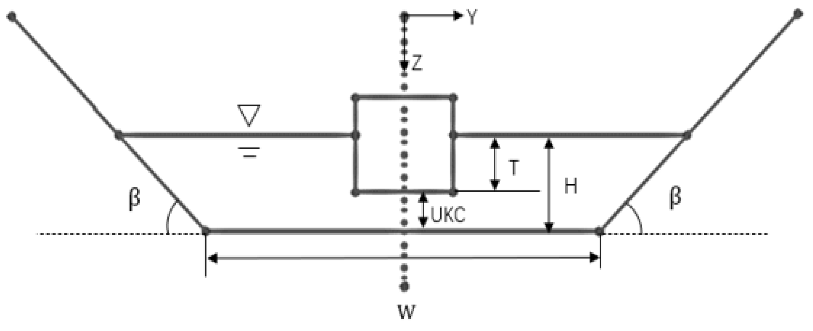
3.1. Ship Geometry

In the numerical simulations, the actual ship model is firstly imported into STARCCM+ and scaled with scale factors 0.04012, 0.03947, and 0.04 in x, y, z directions, respectively. The main properties of full scale for the real ship and model scale for the model ship are depicted in

Table 1. Main parameters of the inland ship.

	Length between Perpendiculars, Lpp/m	Beam, B/m	Moulded Depth, H/m	Draft, T/m	Block Coefficient, ${\mathit{C}}_{\mathit{b}}$	Wetted Surface, $\frac{{\mathit{W}}_{\mathit{s}}}{{\mathit{m}}^2}$	Cross Area of Ship, $\frac{{\mathit{C}}_{\mathit{s}}}{{\mathit{m}}^2}$
full scale	134.58	11.4	6	2.5	0.899	2104.8	34.114
model scale	5.4	0.45	0.24	0.1	0.899	3.367	0.045

. After transforming the real ship, the mass center of the model ship is situated at (2.7, 0, 0.096879).

3.2. Simulation Cases

All the cases are deemed in restricted curved channel, and the details of four different configuration groups (Config. A to D) are illustrated in

Table 2. Simulation cases in curved configurations.

	Config. A	Config. B	Config. C	Config. D
	Channel Radius Variation	Bank Slope Angle Variation	Ship Type Variation	Current Velocity Variation
Total simulation case quantity	4	4	5	8
h/T	1.2	1.2	1.2	1.2
Channel radius, R/m	12.52, 17.72, 23.28, 28.48	17.72	17.72	17.72
Ship speed, ${\mathrm{V}}_{\mathrm{s}}/{\mathrm{m}\ast \mathrm{s}}^{-1}$	0.6173	0.6173	0.6173	0.6173
Channel bottom width, W/m	2.36	2.36	2.36	2.36
Bank slope, β/°	90	13, 27, 50, 90	90	90
Ship length, Lpp/m	5.4	5.4	1.54, 2.68, 3.6, 4.4, 5.4, 7.2	5.4
Ship beam, B/m	0.45	0.45	0.202, 0.328, 0.38, 0.45, 0.45, 0.45	0.45
Current velocity, ${\mathrm{V}}_{\mathrm{c}}/{\mathrm{m}\ast \mathrm{s}}^{-1}$	0	0	0	0.1, 0.15, 0.2, 0.25

with an appropriate cross-section view of the configuration illustrated in Figure 1. Config. A is employed to evaluate the effect of channel radius on ship hydrodynamics, where only a series of channel radius variations exist but the other conditions are kept both constant and severe. Similarly, the other configuration groups namely Config. B, Config. C, and Config. D are set in the same way. So, in total, more than 20 simulations are investigated.

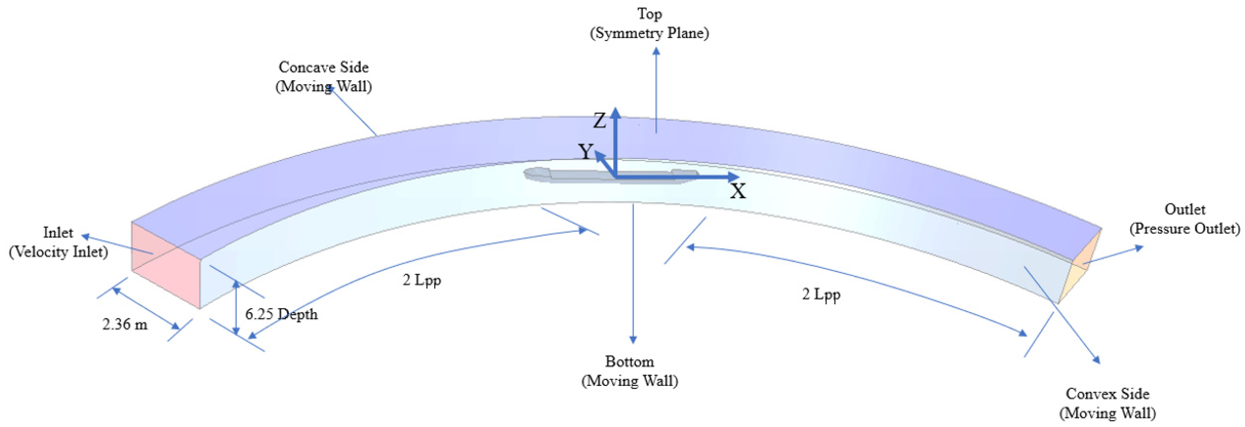
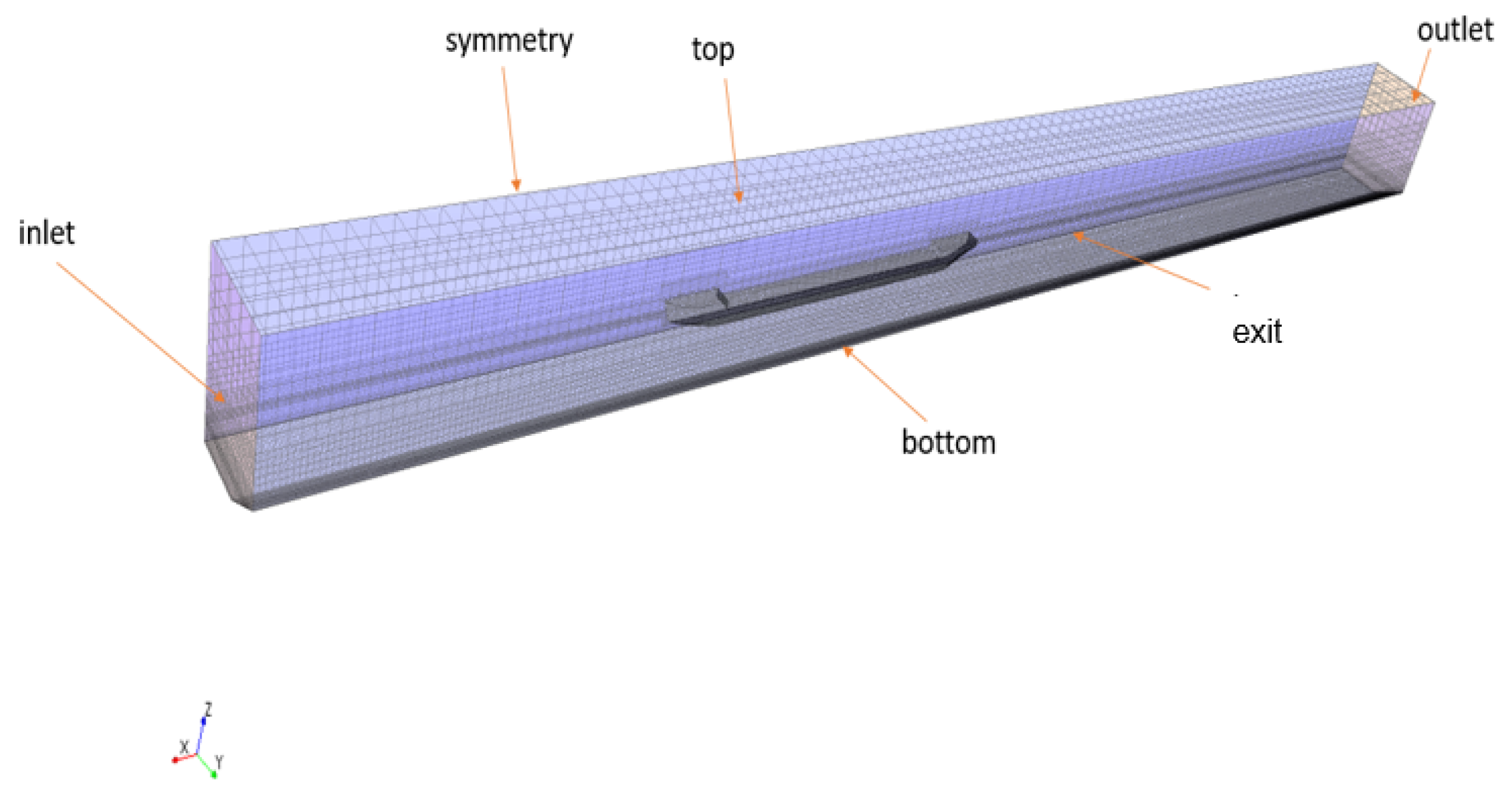
3.3. Computational Domain and Boundary Conditions

A general view of the computational domain with the whole ship model is depicted in Figure 2, which takes the channel of radius 17.72 m for example. The model ship is located in the middle of the curved channel where there is twice L_pp length between the inlet and ship stem, and between the ship stern and the outlet of the domain, respectively, and this will be able to eliminate the influence of any reflected waves at the outlet. Moreover, the height of the fluid domain is 6.25 times the ship depth, and the fairway bottom width is 2.36 m for all the simulations. The bend channels are extracted from a circle with different radius’ (17.72 m, 23.28 m, 28.48 m, respectively) in this research, the total length of which is five times the ship length. The cross-section of the arc channel in the simulations without bank slopes is rectangular whose height is 6.25 times ship height, and the form of it remains constant all along the channel. However, it should be mentioned that the form of the channel cross-section in the simulation groups with bank slopes is trapezoidal, where all the other configuration conditions are the same as those mentioned above.

It should be noted that the whole curved computational domain is rotating around a particular fixed point, which is both the ship’s turning center and the center of the arc channel. The rotation motion is rendered to the meshes in the domain with the same rotation rate as that of the ship, whereas the model ship is fixed in the domain and there is no speed set to the current and wind. Due to the asymmetry of the computational domain and flow around the ship, the entire ship model is simulated in this study without the center plane symmetry. Furthermore, the inlet and outlet are a set velocity inlet and pressure outlet, respectively. The no-slip wall boundary condition is selected for the bottom, concave side, and convex side. Moreover, the top is chosen as a symmetry boundary condition so that the normal component velocity is explicitly set to zero and the prism layer on them can be eliminated. It is worth mentioning that throughout all the cases, to prevent wave reflection from the walls, the VOF wave damping capability of the software is applied to the solution domain with a damping length equal to 5 m. Additionally, a fixed time step that equals 0.05 s is selected for all the simulations.

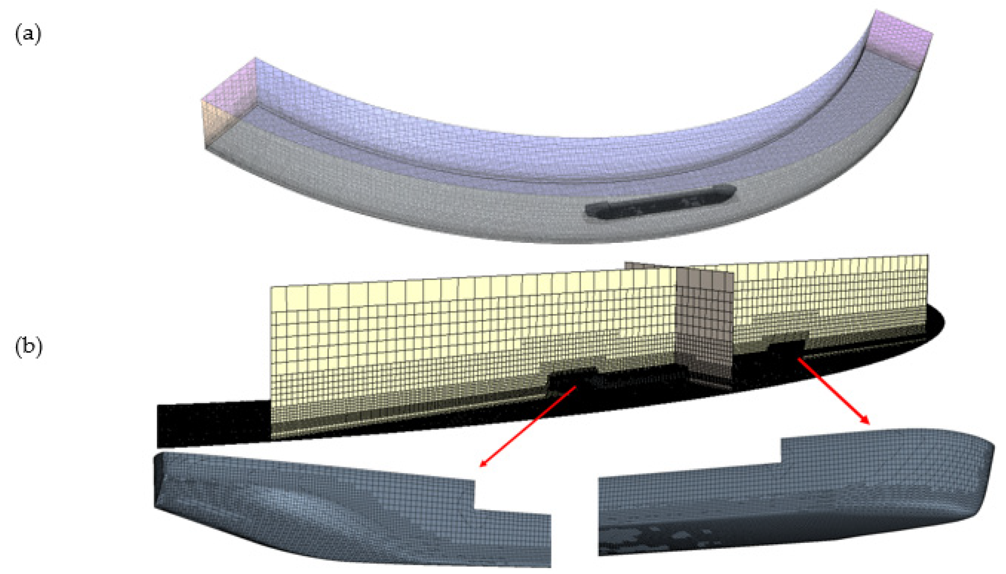
3.4. Mesh Generation and Sensitivity Analysis Test

Mesh generation is carried out with the automated meshing technique in STARCCM+. Trimmed meshes are used to create a high-quality grid for complicated geometric profiles. On the other hand, in viscous fluid, there exists a boundary layer on the body owing to the no-slip boundary condition. This boundary layer ought to be meshed more precisely to capture the near-wall flow accurately, which is critical in measuring forces and flow characteristics. Thus, prismatic meshes incorporating six prism layers with a growth factor of 1.5 are generated on the surface in order to correctly capture the boundary layer and ensure a higher degree of accuracy for the flow solution. The non-dimensional wall distance $y^{+}$ is lower than 1 for all simulations. Especially, a mesh refinement using volumetric controls is applied on the free surface to achieve a proper wave propagation in the domain, and on the underwater ship hull due to the more complex geometry of the ship under the free surface, by doing which the calculation accuracy can be improved. At the same time, the grids far from the ship hull are coarsened by way of surface controls. In this study, to avoid unexpected mesh transitions between the refinements, a slow growth rate is utilized so as to allow the mesher to use several cell layers per transition to facilitate a gradual mesh transition.

After that, a mesh sensitivity analysis test is conducted to show the difficulty of obtaining converged outcomes and to select the most appropriate mesh quality in curvature-effect calculations. In this test, the parameter refinement ratio between two adjacent sizes is $\sqrt{2}$ according to ITTC [26]. The lowest depth to draft ratio (i.e., h/T = 1.2), the shortest channel radius (i.e., R = 17.72 m) and a relatively high ship speed (i.e., Vs = 0.6173 m/s) in this work are chosen as the simulation conditions. Based on this, the predicted hydrodynamic force and moment including resistance force, sway force, and yaw moment denoted by $X$, $Y$, $N$ are showed in Figure 3. The numerical results are then transformed into non-dimensional longitudinal resistance $X^{\prime }$, sway force $Y^{\prime }$, and yaw moment $N^{\prime }$, which are normalized according to:

$$X^{\prime }=\frac{X}{0.5\rho V^2 L_{pp} T}, Y^{\prime }=\frac{Y}{0.5\rho V^2 L_{pp} T}, N^{\prime }=\frac{N}{0.5\rho V^2 L_{pp}{}^2 T}$$

(3)

To analyze the results, the recommended procedures for the numerical uncertainty estimation proposed by ITTC are adopted. Firstly, the convergence ratio $R_i$ is defined using the changes between medium-fine ${\epsilon }_{21}$ and coarse-medium ${\epsilon }_{32}$ solutions, that is

$$R_i=\frac{{\epsilon }_{21}}{{\epsilon }_{32}}$$

(4)

The convergence conditions are judged:

(a)

$0<R_i<1$ refers to monotonic convergence

(b)

$R_i<0$ refers to oscillatory convergence

(c)

$R_i>1$ refers to divergence

Secondly, the numerical error ${\delta }_i$ and order of accuracy $P_i$ are estimated by Equations (5) and (6):

$${\delta }_i=\frac{{\epsilon }_{21}}{r_i{}^{P_i}-1}$$

(5)

$$P_i=\frac{\ln \left({\epsilon }_{32}/{\epsilon }_{21}\right)}{\ln \left(r_i\right)}$$

(6)

where $r_i$ is refinement ratio of grid.

Then if the convergence condition is (a), uncertainty is evaluated according to Equations (7) and (8):

$$U_i=\left\{\begin{array}{c}\left[9.6{\left(1-C_i\right)}^2+1.1\right]\left|{\delta }_i\right|, \left|1-C_i\right|<0.125 \\ \left[2\left|1-C_i\right|+1\right]\left|{\delta }_i\right|, \left|1-C_i\right|\ge 0.125\end{array}\right\}$$

(7)

$$C_i=\frac{r_i{}^{P_i}-1}{r_i{}^{P_{iest}}-1}$$

(8)

where $P_{iest}$ is an approximated value for the limiting order of precision of the first term as spacing size goes to zero, and here it is set two.

If the convergence condition is (b), uncertainty is determined based on oscillation maximums $S_U$ and minimums $S_L$ by $U_i=0.5\left(S_U-S_L\right)$.

The verification results for $X^{\prime }$, $Y^{\prime }$, $N^{\prime }$ are displayed in

Table 3. Mesh verification results and analysis for $X^{\prime }$, $Y^{\prime }$, $N^{\prime }$.

No.	Elements	${\mathit{X}}^{\prime }$	${\mathit{Y}}^{\prime }$	${\mathit{N}}^{\prime }$
Grid 1	4,876,092	0.09395155	0.022136149	−0.028939255
Grid 2	1,371,356	0.094133305	0.029066149	−0.030531812
Grid 3	518,558	0.098757841	0.043988489	−0.025078636
	$R_i$	0.039302228	0.464404351	−0.292042116
	Convergence condition	Monotonic	Monotonic	Oscillatory
	$C_i$	24.47976382	1.15401605	—
	${\delta }_i$	7.42469 × ${10}^{-6}$	0.006005115	—
	$P_i$	9.34256	2.214058	—
	$U_i$	0.000356084	0.007854884	0.002726588

. In the selected grid sets, $X^{\prime }$ and $Y^{\prime }$ are monotonic convergence, whereas $N^{\prime }$ is oscillatory convergence. The mesh uncertainty of $X^{\prime }$,$Y^{\prime }$, and $N^{\prime }$ for all three grid settings are below 1%, based on which we can support our results to a precise degree. In view of the computational efficiency, Grid 2 is a reasonable balance between estimation time and solution precision. Therefore, Grid 2 setting is chosen to be applied to the following simulations. The mesh scene of the computational domain (R = 17.72 m) is showed in Figure 4 as an example.

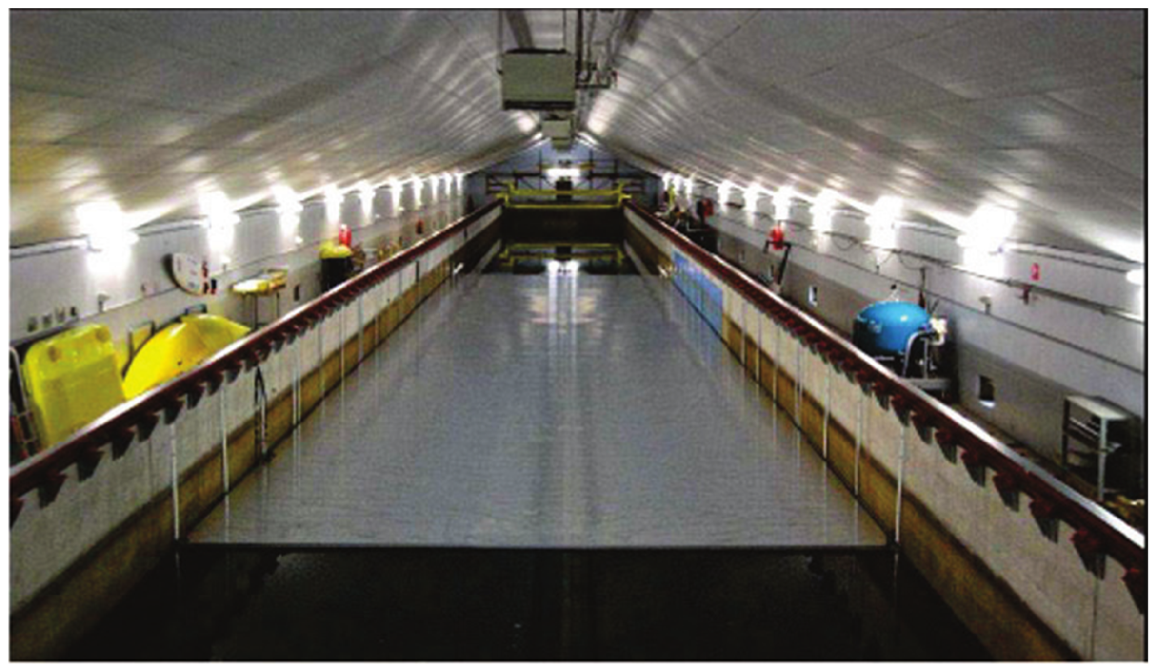
3.5. Validation of the CFD Model

The validation test was conducted with the same ship model in a rectangular channel, and the computational domain is illustrated in Figure 5. The ship speeds equal to those from experiments are rendered to the current and wind at the inlet, and then the ship is equivalent to navigating at the same experimental speeds. The resistances calculated from simulations are compared with those from the experiments that were conducted in the towing tank of Liege university (See Figure 6). The length of the towing tank is 100 m, width is 6 m, and depth is 3.5 m. This aims at demonstrating the reliability of the CFD model in this work. In this study, the scaled model is simulated fixed in a confined channel which is the same as that in the experiment, and due to the fact that there will be a large number of meshes generated and the geometry of the ship model and the fluid domain are strictly symmetric as well, only half the ship model is simulated in STARCCM+ for the sake of economizing time using the symmetry boundary condition. In total, more than 1 million cells are generated.

Three sets of different ship speeds ranging from 0.335 m/s to 0.575 m/s are selected in this numerical simulation and the resistances in x-direction are compared with those in experiments, respectively. Stemming from the confinement of the channel and the very small UKC (under keel clearance) allowed for, it takes all of the three sets of simulations a long time-step to attain convergence. According to the resistance report output, the results of these simulations with those from experiments are compared (see

Table 4. Comparison of resistance between simulation and experiment.

Ship Speed [m/s]	Resistance of Numerical Simulation [N]	Resistance of Experiment/2 [N]	Errors [%]
0.335	0.690084	0.659	4.7168%
0.4485	1.23664	1.194	3.5712%
0.575	2.15804	2.124	1.6026%

).

From Table 4, only slight errors occur between the results from experiments and simulations, which are within 5% for all the three sets selected. Based on this, a good agreement between experiments and numerical simulations can be seen from the results. The CFD results tend to overrate the magnitude of the expected resistance, compared to the towing tank experiments. It should be noted that the standard deviations of the experimental resistance results should be within the range of 5%. Therefore, the validation against the experiments can be considered approved.

4. Results and Discussion

According to the validation test above, it is shown that the CFD model can estimate the resistance with satisfactory accuracy. In this section, the results based on the cases in Table 2 are presented and analyzed to study the curvature effect on ship hydrodynamics and maneuverability. All the simulation results for $X$, $Y$, $N$ are exhibited in non-dimensional forms denoted by $X^{\prime }$, $Y^{\prime }$, $N^{\prime }$. The positive directions of $X^{\prime }$ and $Y^{\prime }$ are the same as the positive directions of x and y coordinate axes, and the positive direction for $N^{\prime }$ is counter-clockwise on paper. At the same time, the pressure and viscous components for the hydrodynamic forces and moment are displayed separately, since the total resistance or sway forces are both composed of pressure force and frictional force, that is $F_t=F_p+F_f$, where $F_t$ is the total force, $F_p$ is the pressure force, and $F_f$ is the frictional force. (prime ‘p’ and ‘f’ indicate pressure and friction respectively for the text below)

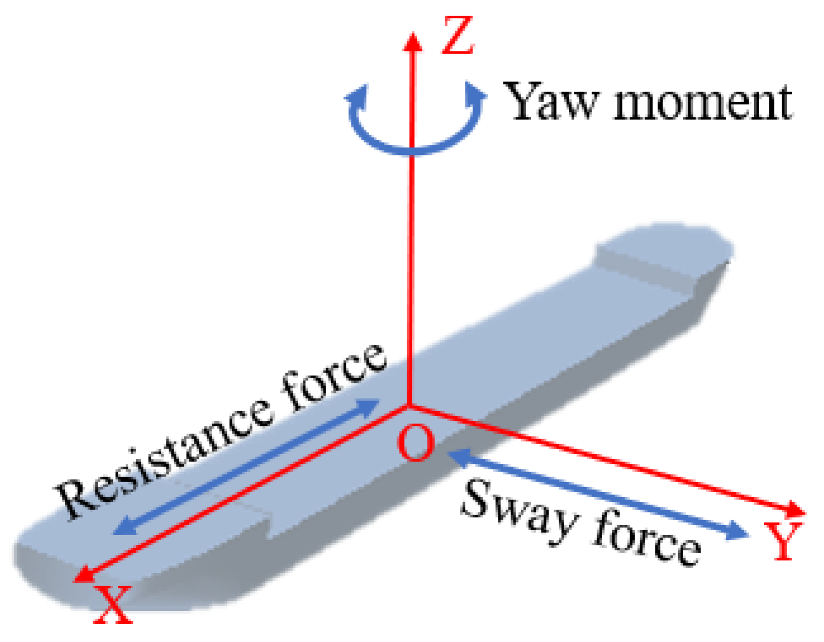
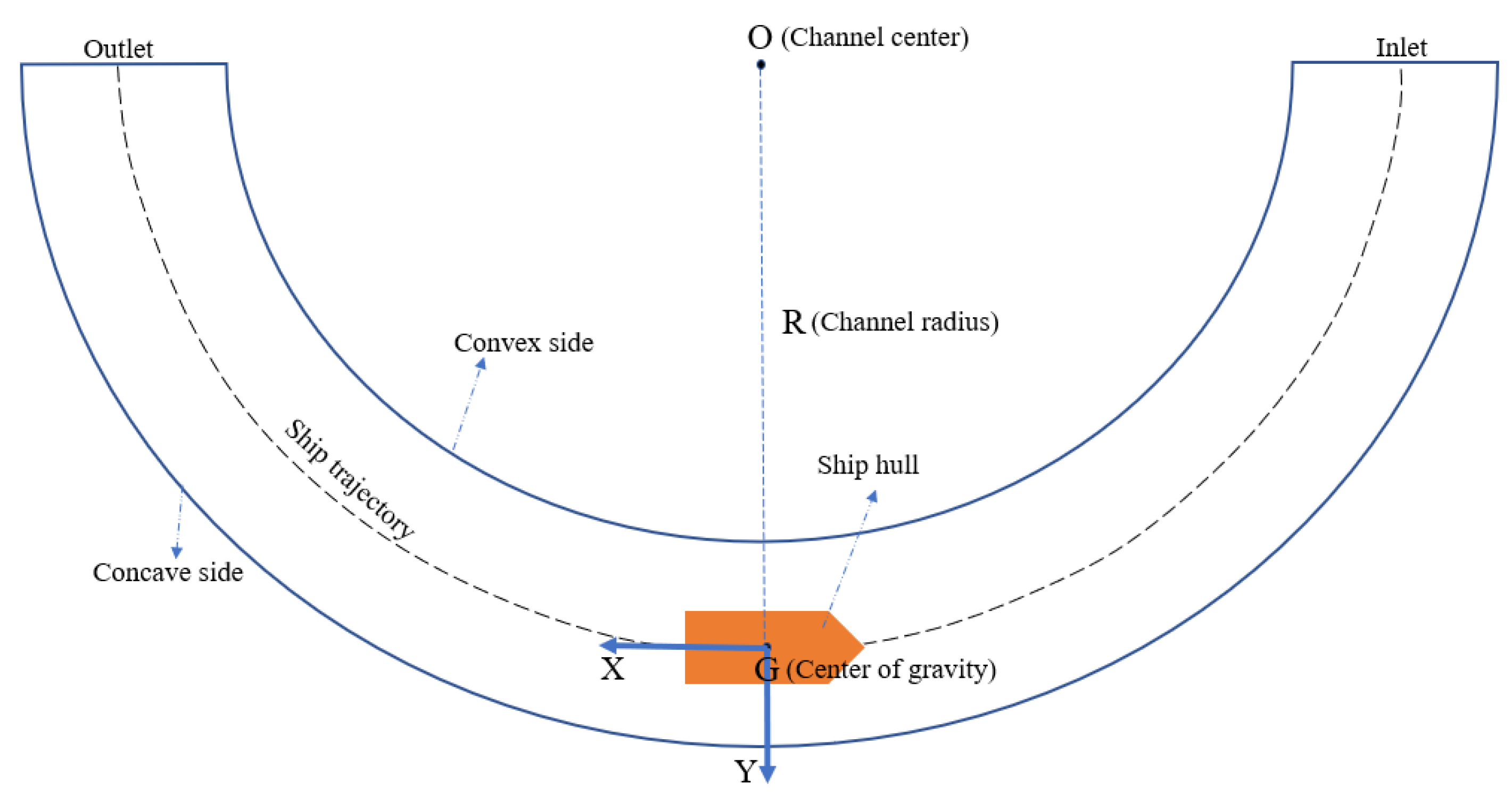
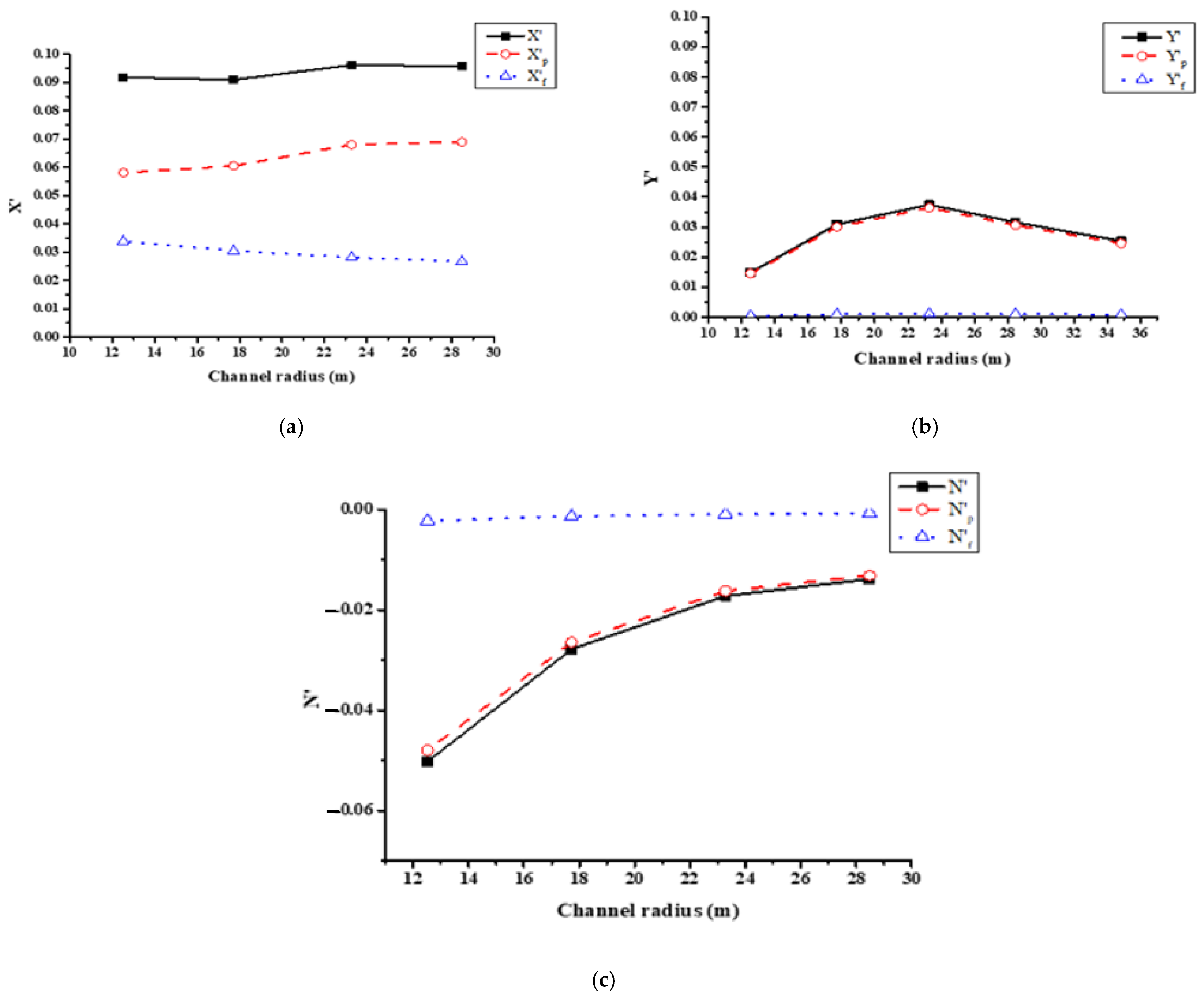
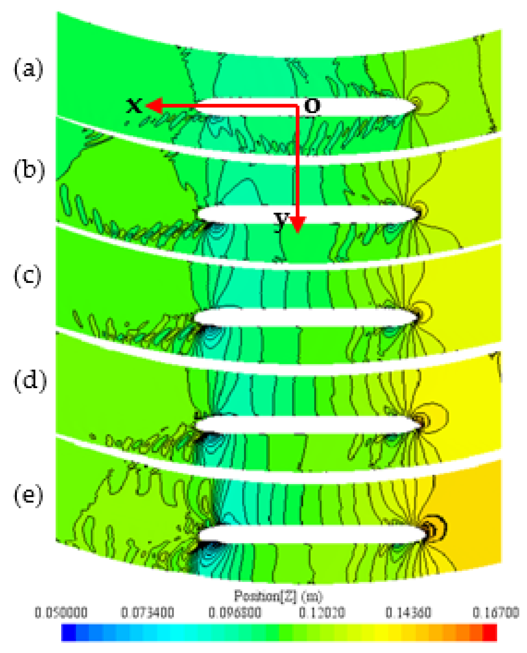
4.1. Effect of Channel Radius® on Flow Behavior and Hydrodynamic Forces and Moment of the Ship

Section 4.1 explains the impact that channel radius (R) exerts on ship hydrodynamics. This work is based on the simulations of Config. A in Table 2. A common sense is that the smaller the R is, the larger the channel curvature is under a constant arc length. R is defined as the radius of ship trajectory, which is depicted in Figure 7.

Figure 8 displays the hydrodynamic forces and moments of the ship in channels with different radiuses. As the R grows, $X^{\prime }$ slightly increases (see Figure 8a), and $X_p^{\prime }$ is nearly twice as large as $X_f^{\prime }$. According to Figure 9, waves generated around the convex bank are becoming more serious during this process, which leads to the increase in $X_p^{\prime }$. Beyond that, no distinct difference in wave profiles can be observed. Moreover, the curvature of streamlines is large under the small R according to Figure 10a, and this means that the mainstream flows near the concave bank passing through a small flow area. At the same time, the curvature of the streamlines is diminishing as the R grows, and consequently the flow area will enlarge. Thus, the flow velocity around the ship will descend according to Venturi effect, which contributes to the decrease in $X_f^{\prime }$.

To verify the tendency of $Y^{\prime }$, another configuration of R = 34.84 is added to Figure 8b. As the R grows, $Y^{\prime }$ increases for the R below a critical value 23.28 m, but the increasing rate is declining. After the R exceeds the critical value, $Y^{\prime }$ starts decreasing. According to Figure 10, the mainstream flows around the concave bank when passing through the curved section for the small R. The ship is therefore subjected to $Y^{\prime }$ pointing towards the concave bank. However, the curvature of streamlines is decreasing as the R grows, leading to a smaller $Y^{\prime }$. Thus, the upward trend in $Y^{\prime }$ is gradually slowing down for 17.72 m < R < 23.28 m. Afterwards, $Y^{\prime }$ starts decreasing after the R surpasses the critical value 23.28 m, since the curvature of streamlines is no longer evident for R > 23.28 m. Moreover, $Y_p^{\prime }$ dominates all the time.

A particularly pronounced effect of the R on $N^{\prime }$ can be observed under the small R according to Figure 8c. $N^{\prime }$ descends fast as the R grows, and meanwhile, the magnitude of change of $N^{\prime }$ is more considerable under the smaller R. However, the decreasing rate is slowing down with the R increasing. For the R < 17.72 m, a rapid descending rate of 42.6% in $N^{\prime }$ can be viewed with the R increasing. This dramatic change is caused by the more intense loop circulation under such a small R (See Figure 10a). Caused by this, $N^{\prime }$ is getting larger in channels with smaller radiuses. Thus, ships are more liable to drift in curved channels with a small R, and a pilot must steer the ship constantly to correct the ship’s course in this case. $N_p^{\prime }$ dominates in $N^{\prime }$ with the frictional component approaching 0, which is caused by bow and stern effect.

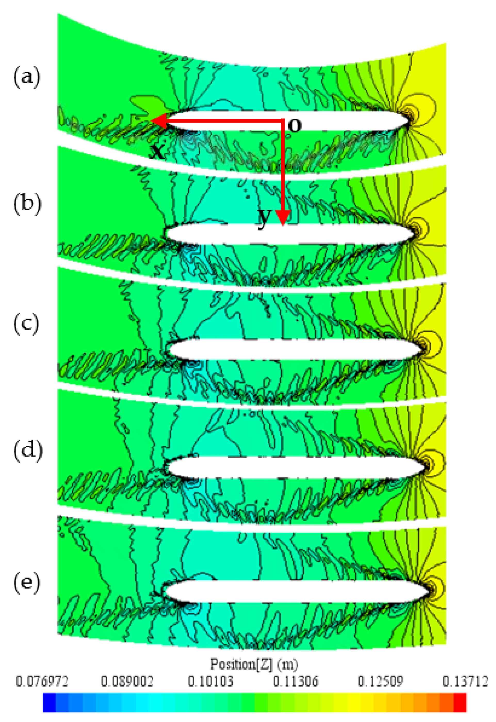
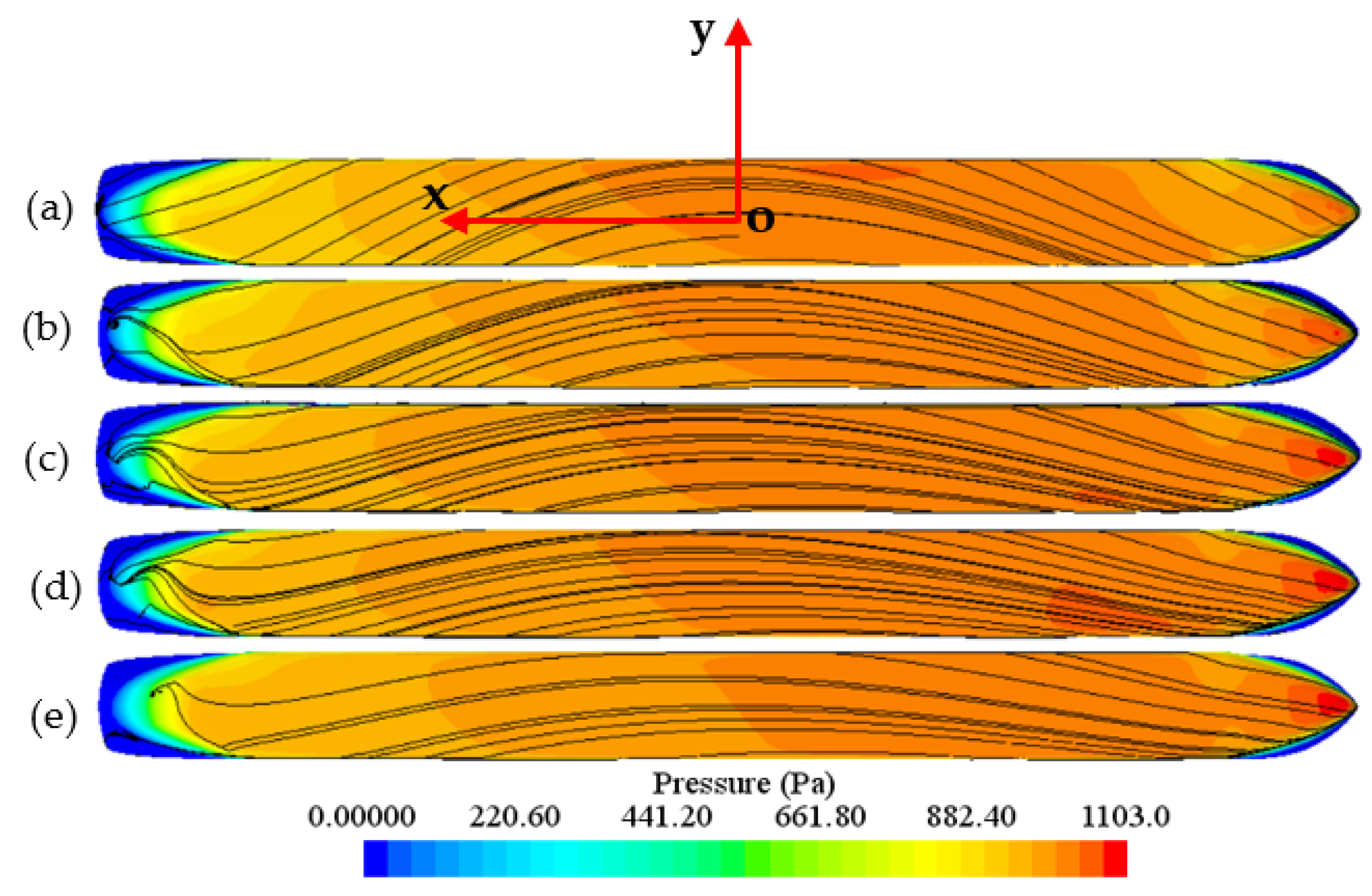
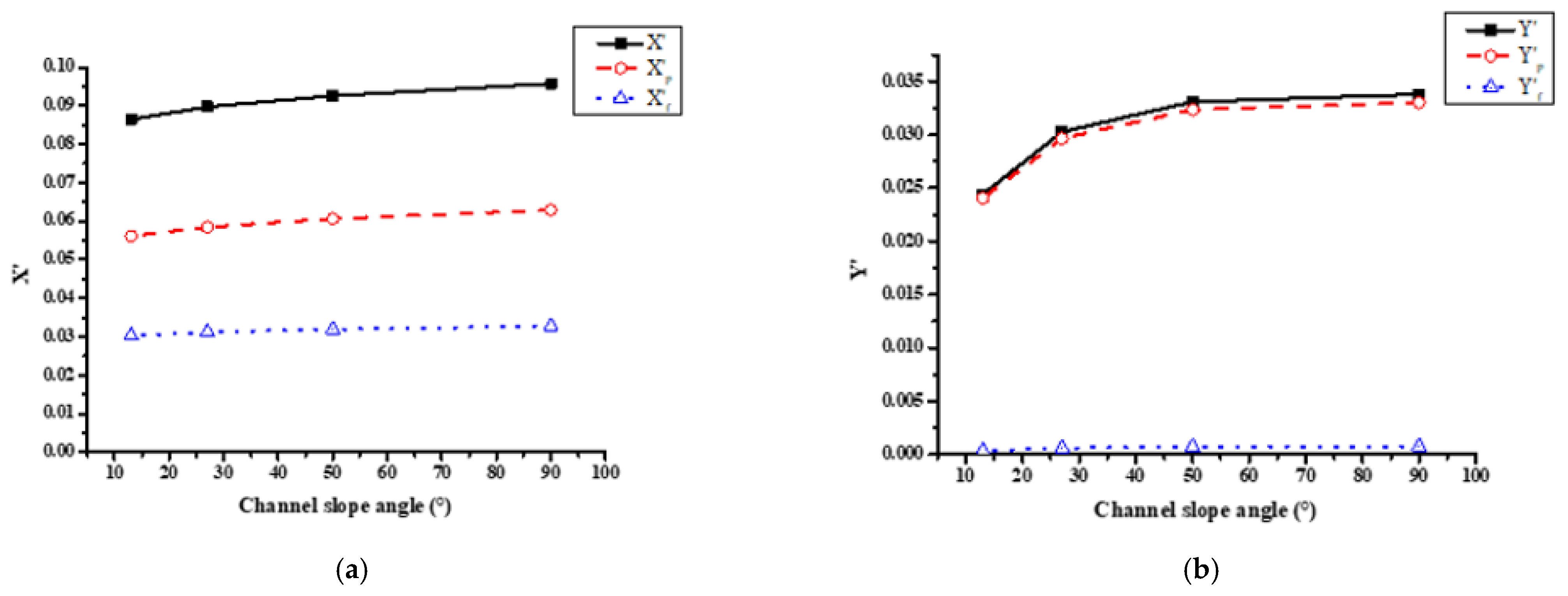
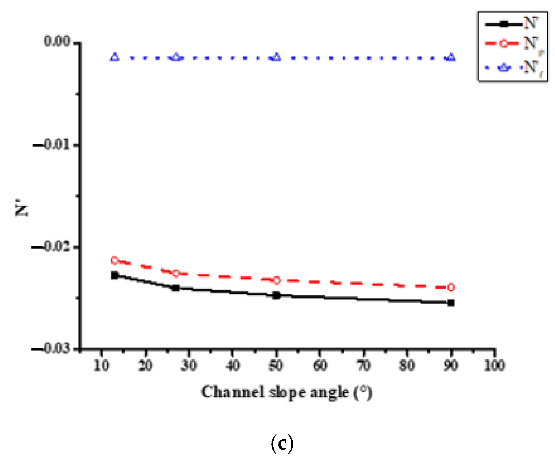
4.2. Effect of Bank Slope Angle(β) on Flow Behavior and Hydrodynamic Forces and Moment of the Ship

This section analyzes the effect brought by β on ship hydrodynamics, which is based on the simulations from Config. B in Table 2. The channel bottom width(W) is constant during this process.

According to Figure 11, $X^{\prime }$ slightly increases as β grows, and $X_p^{\prime }$ is around twice as large as $X_f^{\prime }$. Ship waves are more generated as β grows, the change of which is particularly noticeable for β < 27° (see Figure 12a,b), which contributes to the increase in $X_p^{\prime }$. Meanwhile, the wave elevation is decreasing during this procedure, and consequently the pressure around the ship is descending (see Figure 13). Trim by stern will occur more easily for small slope angles. However, the streamlines are hardly affected as function of β.

There exists a critical value for the effect of β (50° in this work) on $Y^{\prime }$ and $N^{\prime }$. $Y^{\prime }$ increases by a comparatively large extent (increasing rate 23.95%) for β < 27°. Its direction points towards the concave bank, which can be noticed from the flowing direction of streamlines. Then, this growing rate slows down after β exceeds 27°, especially negligible change can be observed in $Y^{\prime }$ for β > 50° (increasing rate 2.1%). For β > 27°, the wave profile becomes serious and nearly does not vary as a function of β. Bow waves around the concave bank will be backed up by the bank to act on the ship hull, applying a force towards the convex bank. This diminishes the force growth. On the other hand, the restraining effect of bank on ships is strengthening as β grows, but this effect has gradually come to a limit after β exceeds a critical value 50°. $Y_p^{\prime }$ dominates all the time with $Y_f^{\prime }$ around 0, which is caused by the bow and stern effect. As β grows, $N^{\prime }$ increases marginally with an increasing rate only 5.56% for β < 27°, but a similar phenomenon occurs with $N^{\prime }$ that the growing rate in $N^{\prime }$ is decreasing. Especially for β > 50°, $N^{\prime }$ hardly increases. $N_p^{\prime }$ dominates during this process.

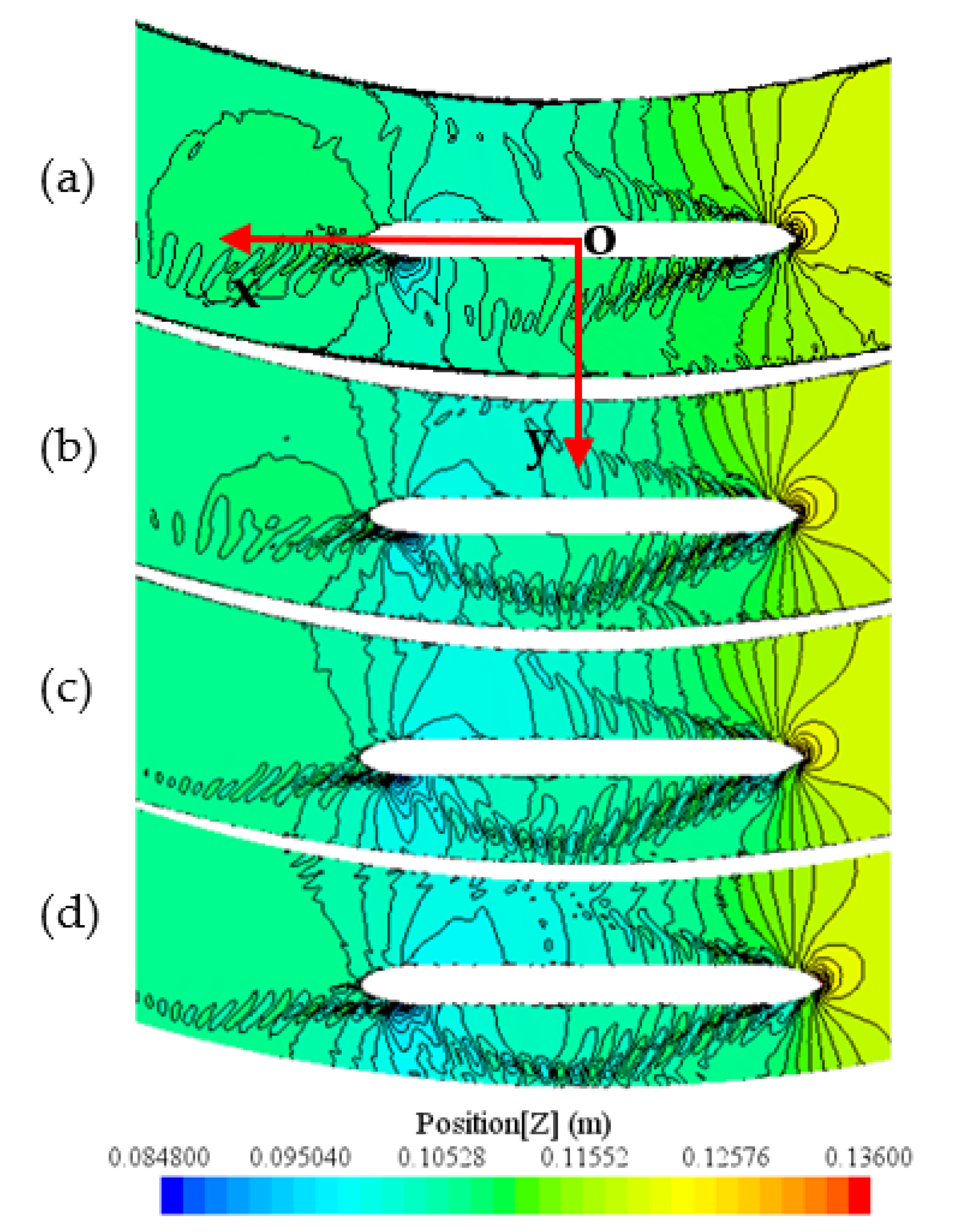
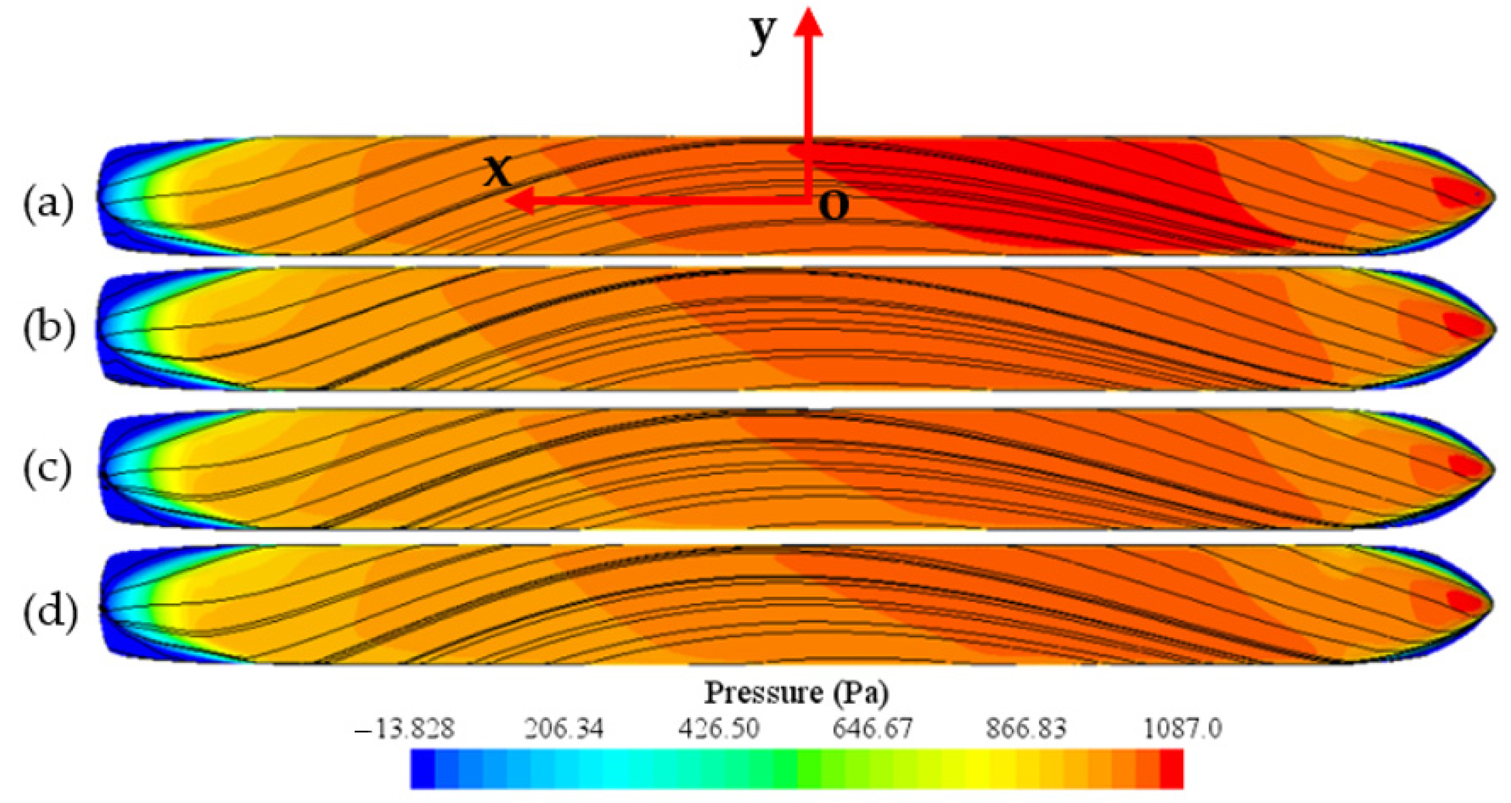
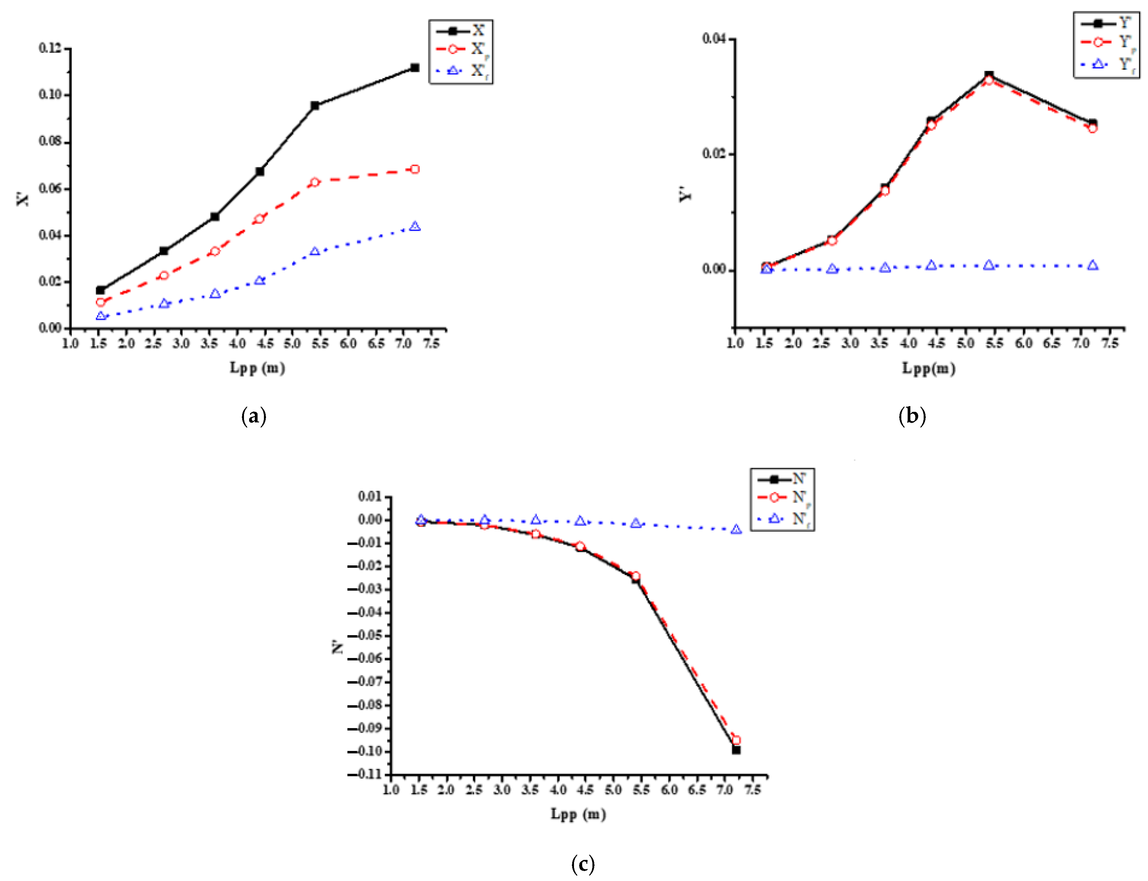
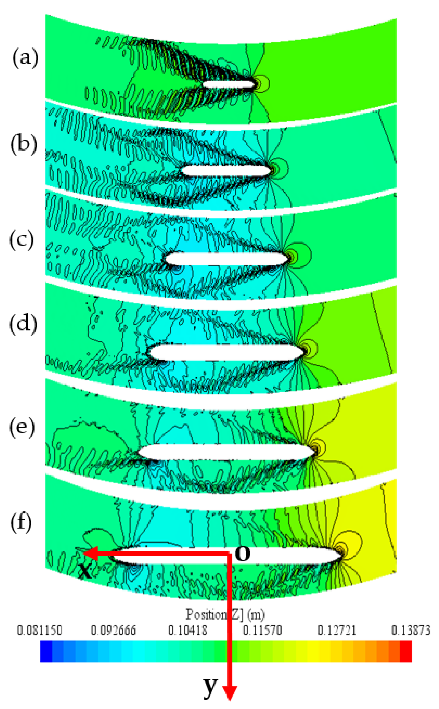
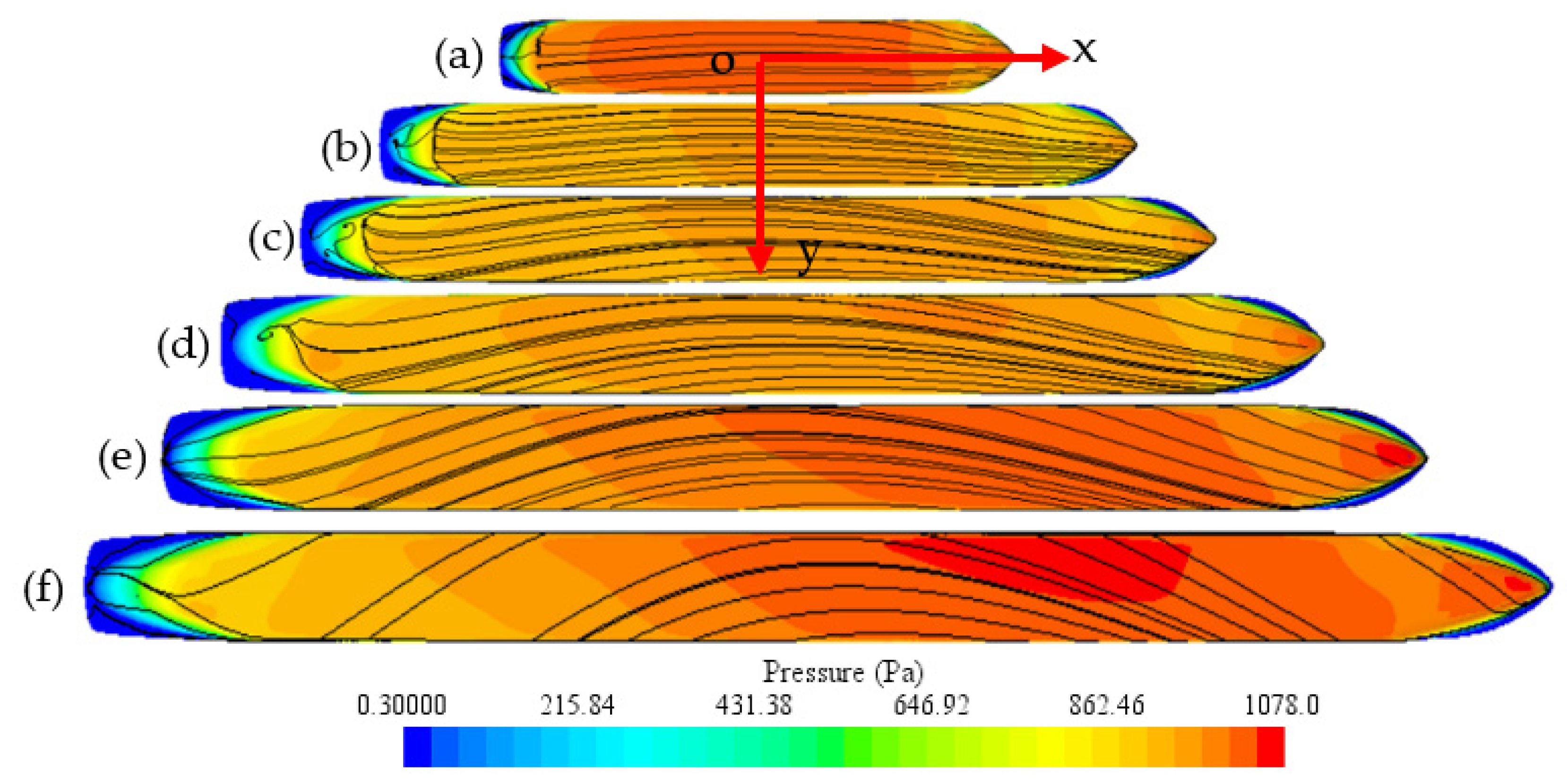
4.3. Effect of Ship Type on Flow Behavior and Hydrodynamic Forces and Moment of the Ship

The curved channels will limit the size of ships that pass the curves. In this section, different inland ship types (different ship length and beam) are selected, such as Péniche Freycinet (classe I), Dortmund-EMS-Kanaal (DEK) (classe III), Rheine Herne Kanaal(RHK) (classe IV), and so on. Among the different ship types, ship length is the most influential factor in narrow bending zones. Thus, this section analyzes the effect brought by ship type (chiefly ship length) on ship hydrodynamics, which is based on the simulations from Config. C in Table 2.

As L_pp grows, $X^{\prime }$ increases more and more rapdily for L_pp < 5.4 m, which is due to the increase in both $X_p^{\prime }$ and $X_f^{\prime }$ (see Figure 14). This is because of the larger contacting area between the ship hull and current during this process. In addition, bow waves generated around the convex bank and stern waves are both becoming less serious.

According to the free surface change at the bow (see Figure 15a–f), free surface elevation around the convex bank is becoming higher than that around the concave bank, whereas the free levels around the concave bank are proximately always the same. Moreover, the water level at the stern nearly keeps constant during this process. $Y^{\prime }$ consequently increases faster for L_pp < 5.4 m. However, the streamline curvature of flow can also be influenced a lot by the change of ship length, and will become extremely larger when the ship is long enough (from Figure 16e,f). Therefore, $Y^{\prime }$ can be noticed decreasing from L_pp = 5.4 m to L_pp = 7.2 m. Owing to the larger curvature of mainstream, there is relatively less part of mainstream flowing through the bottom of the hull, and $X^{\prime }$ also grows slowly from L_pp = 5.4 m to L_pp = 7.2 m as a result.

The free level change mentioned above, combined with the larger curvature of streamlines around the ship in the case of large L_pp (signifying that stronger spriral flow exists) will cause $N^{\prime }$ to increase more and more rapidly as L_pp grows. Therefore, the long ship is more prone to drifting in curved channels. Due to different ship beams of the models, pressure distributed on the ship bottom (see Figure 16) and wave elevation (see Figure 17) around the hull both show a trend of decreasing first and then increasing.

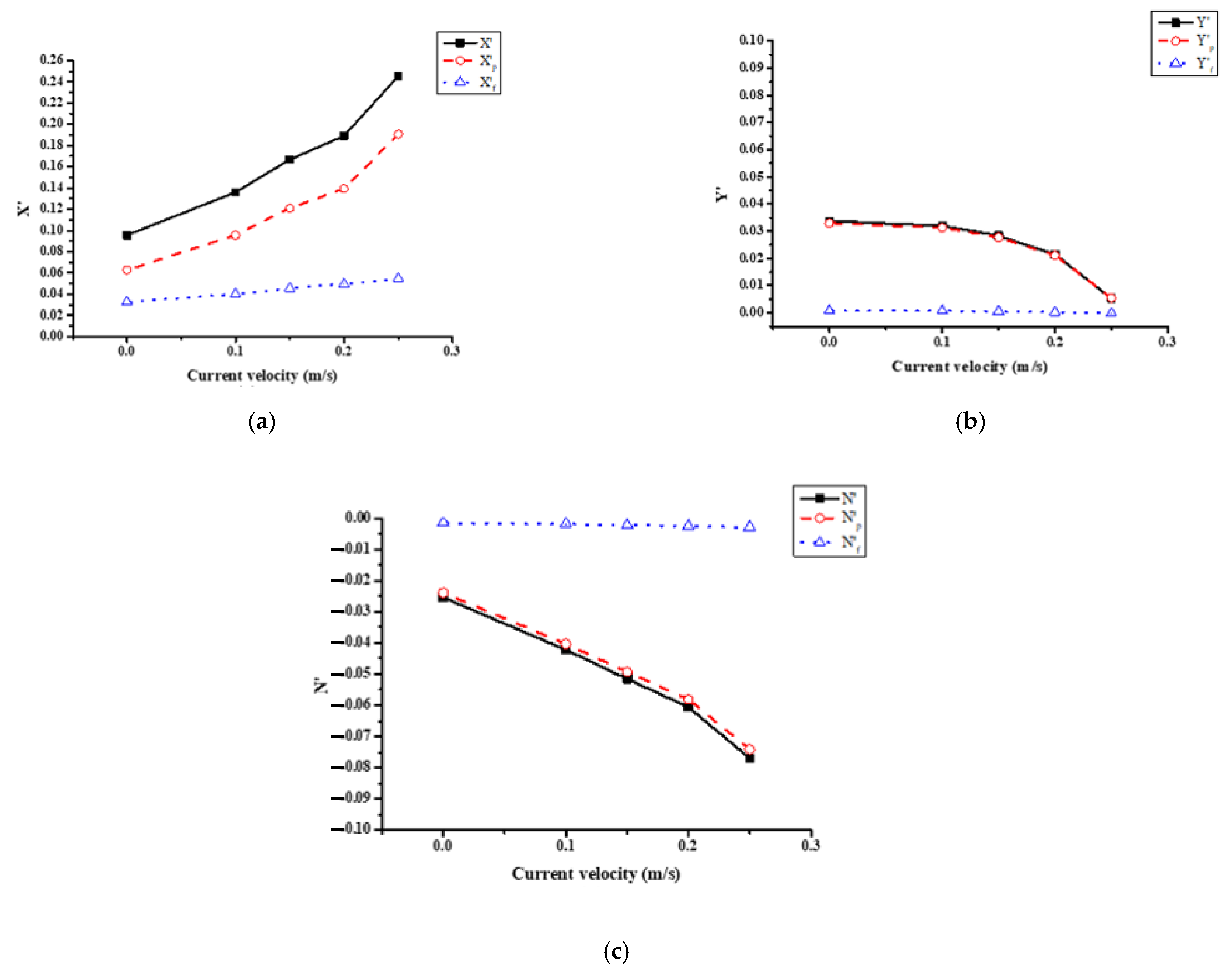
4.4. Current Effect on Flow Behavior and Hydrodynamic Forces and Moment of the Ship

In real rivers, the current normally has a certain speed and can therefore impact the movement and maneuverability of a ship. In this section, the currents with velocities ranging from 0.1 m/s to 0.25 m/s were set at Inlet of the fluid domain, for which the effect by currents can be researched.

$X^{\prime }$ increases faster and faster as V_c (current velocity) grows, which is mostly due to the increase in $X_p^{\prime }$ (see Figure 18a). Currents will obviously cause more resistance to the ship as V_c increases. What should be noticed is that stern waves are obviously becoming more serious during this process; however, bow waves are disappearing due to the hydrolic jump according to Figure 19. At the same time, the pressure distributed around the ship bow is increasing, while conversely, the pressure near the ship stern is decreasing (see Figure 20). So, the increase in V_c will result in a greater hydrostatic pressure difference between the bow and stern. Nevertheless, the curvature of streamlines is hardly affected as function of V_c.

$Y^{\prime }$ decreases slightly for V_c below 0.2 m/s, but it starts decreasing fast after V_c exceeds this critical value (decreasing rate 74.77%). From Figure 19a–e, wave elevation around the concave bank can be noticed gradually higher than that around the convex bank.

$N^{\prime }$ increases fast as Vc grows. Considering the almost unchanged current curvature, a larger yaw moment will be caused when a current with higher velocity passes through the ship hull.

5. Conclusions

In this paper, numerical simulations based on implicit unsteady equations and the realizable K-Epsilon turbulence model were performed to investigate the curvature effect of curved channels on ship hydrodynamics. A verification study via grid convergence analysis according to ITTC in a curved channel was performed to select the most appropriate grid setting, and also validation research in a straight channel validated by experiment results was conducted to prove that the numerical model estimates hydrodynamic forces correctly. A range of specific parameters incorporating channel radius, bank slope angle, ship type, and current speed were selected to study the effects of changes in these parameters on $X^{\prime }$, $Y^{\prime }$, $N^{\prime }$. The results are as follows:

(a) As the channel radius (R) grows, $X^{\prime }$ increases slightly, and $X_p^{\prime }$ is nearly twice as large as $X_f^{\prime }$. There exists a critical R for $Y^{\prime }$. $Y^{\prime }$ increases when R is lower than a critical value, but $Y^{\prime }$ descends after the R exceeds this value (behave as Gaussian form). $N^{\prime }$ decreases fast under a small R, while the decreasing rate is slowing down since the spiral flow is becoming weaker during this process. Hence, special attention should be paid while a ship is navigating in curved channels with a small channel radius, as drift induced by $N^{\prime }$ is extremely easy to occur in this case.

(b) Channel slope angle (β) only affects ship hydrodynamics much at small angles, and $X^{\prime }$, $Y^{\prime }$, $N^{\prime }$ increase as the bank gets steeper. The changes in $X^{\prime }$, $Y^{\prime }$, $N^{\prime }$ all seem more obvious when β is lower than a critical value (50 degrees). After that, the restraining effect of β comes to a limit so that ship hydrodynamics will hardly be influenced by the variance of it.

(c) As the ship length (L_pp) grows, $X^{\prime }$ and $Y^{\prime }$ increase gradually faster for ship length (L_pp) lower than the critical value 5.4 m. However, $X^{\prime }$ starts increasing more slowly, while $Y^{\prime }$ decreases when L_pp exceeds this value. $N^{\prime }$ grows increasingly faster during this process. At the bow, the free surface level on convex bank is becoming increasingly higher, whereas it is almost unchanged on the concave bank. At the stern, the water level keeps nearly the same around both bank sides. Moreover, the curvature of the flow streamlines of long ships can be noticed extremely larger than that of short ships.

(d) As current velocity (V_c) grows, $X^{\prime }$ and $N^{\prime }$ both increase faster and faster. However, $Y^{\prime }$ (with its direction towards concave bank) decreases slightly for V_c lower than a critical value 0.2 m/s, exceeding which $Y^{\prime }$ starts decreasing fast. Pressure at the bow is increasing, while it is decreasing at the stern. A trim by stern is much easier to occur at high V_c. Moreover, the hydrolic jump will arise during this process.

References

1. Eskinazi, S.; Yeh, H. An Investigation on Fully Developed Turbulent Flows in a Curved Channel. J. Aeronaut. Sci. 1956, 23, 23–34. [Google Scholar] [CrossRef]
2. De Vriend, H.J. A Mathematical Model of Steady Flow in Curved Shallow Channels. J. Hydraul. Res. 1977, 15, 37–54. [Google Scholar] [CrossRef]
3. Booij, R. Modelling the flow in curved tidal channels and rivers. In Proceedings of the International Conference on Estuaries and Coasts, Hangzhou, China, 9–11 November 2003. [Google Scholar]
4. Blanckaert, K.; De Vriend, H.J. Nonlinear modeling of mean flow redistribution in curved open channels. Water Resour. Res. 2003, 39, 1375. [Google Scholar] [CrossRef]
5. Kalkwijk, J.P.T.; De Vriend, H.J. Computation of the flow in shallow river bends. J. Hydraul. Res. 1980, 18, 327–342. [Google Scholar] [CrossRef]
6. Blanckaert, K. Flow separation at convex banks in open channels. J. Fluid Mech. 2015, 779, 432–467. [Google Scholar] [CrossRef]
7. Nguyen, V.T.; Nestmann, F. Applications of CFD in Hydraulics and River Engineering. Int. J. Comput. Fluid Dyn. 2004, 18, 165–174. [Google Scholar] [CrossRef]
8. Aseperi, O. Dynamics of Flow in River Bends. Ph.D. Thesis, Colorado State University, Fort Collins, CO, USA, 2018. [Google Scholar]
9. Huang, S.-L.; Jia, Y.-F.; Chan, H.-C.; Wang, S.S.Y. Three-Dimensional Numerical Modeling of Secondary Flows in a Wide Curved Channel. J. Hydrodyn. 2009, 21, 758–766. [Google Scholar] [CrossRef]
10. Maslikova, O.Y.; Gritsuk, I.I.; Debol’Skaya, E.I. The effect of flow velocity distribution on matter transport in a curved channel segment with the effect of moving ships taken into account. IOP Conf. Series Earth Environ. Sci. 2019, 321, 012026. [Google Scholar] [CrossRef]
11. Vujičić, S.; Mohović, R.; Tomaš, I. Methodology for Controlling the Ship’s Path during the Turn in Confined Waterways. Pomorstvo 2018, 32, 28–35. [Google Scholar] [CrossRef]
12. Ai, W.Z.; Gan, X.Z. Analysis on Navigation Reliability of Curved Channel. Appl. Mech. Mater. 2013, 275–277, 2816–2820. [Google Scholar] [CrossRef]
13. Ai, W.; Zhang, H.; Zhu, P.; Chi, H. A Study on Safe Ship Navigation in Curved Bridge Channel. J. Coast. Res. 2020, 109, 121–125. [Google Scholar] [CrossRef]
14. Ai, W.; Zhu, P. Navigation Ship’s Drift Angle Determination Method in Curved Channel. J. Coast. Res. 2020, 109, 181–184. [Google Scholar] [CrossRef]
15. Wang, C.H.; Cheng, X.B. Research on Navigable Ship Model Test in Curved Waterway. Appl. Mech. Mater. 2014, 580–583, 1918–1922. [Google Scholar] [CrossRef]
16. Yang, B.; Kaidi, S.; Lefrançois, E. Numerical investigation of curvature effect on ship hydrodynamics in confined curved channels. In Proceedings of the 9th Conference on Computational Methods in Marine Engineering, Edinburgh, UK, 2–4 June 2021; Volume 1. [Google Scholar] [CrossRef]
17. RoyChoudhury, S.; Dash, A.K.; Nagarajan, V.; Sha, O.P. CFD simulations of steady drift and yaw motions in deep and shallow water. Ocean Eng. 2017, 142, 161–184. [Google Scholar] [CrossRef]
18. Bechthold, J.; Kastens, M. Robustness and quality of squat predictions in extreme shallow water conditions based on RANS-calculations. Ocean Eng. 2020, 197, 106780. [Google Scholar] [CrossRef]
19. Shevchuk, I.; Kornev, N. A study of unsteady hydrodynamic effects in the stern area of river cruisers in shallow water. Ship Technol. Res. 2017, 64, 87–105. [Google Scholar] [CrossRef]
20. Zou, L.; Larsson, L. Computational fluid dynamics (CFD) prediction of bank effects including verification and validation. J. Mar. Sci. Technol. 2013, 18, 310–323. [Google Scholar] [CrossRef]
21. Kaidi, S.; Smaoui, H.; Sergent, P. CFD Investigation of Mutual Interaction between Hull, Propellers, and Rudders for an Inland Container Ship in Deep, Very Deep, Shallow, and Very Shallow Waters. J. Waterw. Port Coastal Ocean Eng. 2018, 144, 04018017. [Google Scholar] [CrossRef]
22. Razgallah, I.; Kaidi, S.; Smaoui, H.; Sergent, P. The impact of free surface modelling on hydrodynamic forces for ship navigating in inland waterways: Water depth, drift angle, and ship speed effect. J. Mar. Sci. Technol. 2018, 24, 620–641. [Google Scholar] [CrossRef]
23. Terziev, M.; Tezdogan, T.; Oguz, E.; Gourlay, T.; Demirel, Y.K.; Incecik, A. Numerical investigation of the behaviour and performance of ships advancing through restricted shallow waters. J. Fluids Struct. 2018, 76, 185–215. [Google Scholar] [CrossRef]
24. Du, P.; Ouahsine, A.; Sergent, P.; Hu, H. Resistance and wave characterizations of inland vessels in the fully-confined waterway. Ocean. Eng. 2020, 210, 107580. [Google Scholar] [CrossRef]
25. Du, P.; Ouahsine, A.; Toan, K.T.; Sergent, P. Simulation of ship maneuvering in a confined waterway using a nonlinear model based on optimization techniques. Ocean Eng. 2017, 142, 194–203. [Google Scholar] [CrossRef]
26. Uncertainty Analysis in CFD Verification and Validation Methodology and Procedures. International Towing Tank Conference (ITTC), September 2017. 7.5-03-01-01, pp.1–13. Available online: https://www.ittc.info/media/8153/75-03-01-01.pdf (accessed on 25 July 2022).
Figure 1. Cross section view of the curved configuration.
Jmse 10 01263 g001
Figure 2. Three-dimensional view of the computational domain, its dimensions, and corresponding boundary conditions (R = 17.72 m).
Jmse 10 01263 g002
Figure 3. Motion illustrations of the ship model in this work.
Jmse 10 01263 g003
Figure 4. Mesh scene of the computational domain (R = 17.72 m). (a) Volume mesh scene of the entire computational domain; (b) Volume mesh scene inside the computational domain.
Jmse 10 01263 g004
Figure 5. Computational domain of the validation simulation.
Jmse 10 01263 g005
Figure 6. Towing tank for the experiments in this paper.
Jmse 10 01263 g006
Figure 7. Plane figure of channel setting in this paper.
Jmse 10 01263 g007
Figure 8. Non–dimensional results of channel radius on ship hydrodynamics. (ac): resistance force, sway force, yaw moment.
Jmse 10 01263 g008
Figure 9. Free surface elevation contour of channel radius variation. (ae): Channel radius from 12.52 m to 34.84 m.
Jmse 10 01263 g009
Figure 10. Pressure contours with streamlines of channel radius variation. (ae): Channel radius from 12.52 m to 34.84 m.
Jmse 10 01263 g010
Figure 11. Non–dimensional results of channel slope angle on ship hydrodynamics (ac): resistance force, sway force, yaw moment.
Jmse 10 01263 g011aJmse 10 01263 g011b
Figure 12. Free surface elevation contours of slope angle variation. (ad): slope angle is 13°, 27°, 50°, 90°, respectively.
Jmse 10 01263 g012
Figure 13. Pressure contours with streamlines of slope angle variation. (ad): slope angle is 13°, 27°, 50°, 90°, respectively.
Jmse 10 01263 g013
Figure 14. Non–dimensional results of ship type on ship hydrodynamics (ac): resistance force, sway force, yaw moment.
Jmse 10 01263 g014
Figure 15. Free surface elevation contours of ship type variation. (af): Lpp = 1.54 m, 2.68 m, 3.6 m, 4.4 m, 5.4 m, 7.2 m corresponding beam = 0.202 m, 0.328 m, 0.38 m, 0.45 m, 0.45 m, 0.45 m.
Jmse 10 01263 g015
Figure 16. Pressure contours with streamlines of ship type variation. (af): Lpp = 1.54 m, 2.68 m, 3.6 m, 4.4 m, 5.4 m, 7.2 m corresponding beam = 0.202 m, 0.328 m, 0.38 m, 0.45 m, 0.45 m, 0.45 m.
Jmse 10 01263 g016
Figure 17. Pressure distribution at bow and stern for ship type variation. (af): Lpp = 1.54 m, 2.68 m, 3.6 m, 4.4 m, 5.4 m, 7.2 m; corresponding beam = 0.202 m, 0.328 m, 0.38 m, 0.45 m, 0.45 m, 0.45 m.
Jmse 10 01263 g017
Figure 18. Non–dimensional results of current velocity on ship hydrodynamics (ac): resistance force, sway force, yaw moment.
Jmse 10 01263 g018
Figure 19. Free surface elevation contours of current velocity. (ae): current velocity = 0 m/s, 0.1 m/s, 0.15 m/s, 0.2 m/s, 0.25 m/s.
Jmse 10 01263 g019
Figure 20. Pressure contours with streamlines of current velocity. (ae): current velocity = 0 m/s, 0.1 m/s, 0.15 m/s, 0.2 m/s, 0.25 m/s.
Jmse 10 01263 g020