Investigation of Energy Losses Induced by Non-Uniform Inflow in a Coastal Axial-Flow Pump

Abstract

A non-uniform velocity profile occurs at the inlet of a coastal axial-flow pump which is placed downstream of the forebay with side-intake. As a result, the actual efficiency and head of the pump is dissimilar to the design parameters, and the lack of the theoretical investigation on the relationship between inflow distortion and energy losses restricts the application of the coastal axial-flow pump in the drainage project. In this paper, the unsteady numerical simulation and entropy production theory are employed to obtain the internal flow structure and quantify energy losses, respectively, with three inflow deflection angles ($\theta$ = 0°, 15°, or 30°). It is reported that the best efficiency point (BEP) shifts to large flow rate with $\theta$ increasing, due to the decline of the velocity component in axial direction at the impeller inlet. Therefore, the total entropy production (TEP) of the coastal axial-flow pump rises with $\theta$ increasing under small flow rates, but it decreases with $\theta$ increasing under large flow rates. The high total entropy production rate (TEPR) in the vicinity of the tailing edge of the impeller and guide vanes rises with $\theta$ increasing, caused by the enhanced wake vortex strength. In addition, the high TEPR area near the inlet of outflow conduit rises with $\theta$ increasing, originated from the improvement of secondary vortices intensity.

1. Introduction

Vertical axial-flow pumps have been extensively applied in drainage projects in coastal cities, due to high flow rate and convenient maintenance measures [1,2,3]. Their hydraulic performance is the key to ensure the normal operation of urban water systems. In general, the hydraulic design of a coastal axial-flow pump is based on a purely axial inflow at the inlet section, i.e., a uniform inflow rate. However, some coastal axial-flow pumps need to be installed along narrow watercourses and the coastal axial-flow pump’s inlet is connected to the forebay with side-intake to reduce its footprint. As a result, the inlet section of the coastal axial-flow pump shows a non-uniform velocity profile in the actual application, which leads to the performance deviations compared with the hydraulic design due to the change of angle between inflow and leading edge in the impeller [4,5]. To develop the application prospects of coastal axial-flow pumps in drainage project, the physical connection between the unstable flow structure induced by non-uniform inflow and energy loss characteristics needs to be established.

In recent years, computational fluid dynamic (CFD) techniques have been increasingly used in the design of water jet pumps [6], centrifugal pumps [7,8], pump-turbines [9], and axial-flow pumps [10]. It can rapidly and accurately capture the details of unsteady flow structures induced by non-uniform inflow levels [11] and predict the pump’s performance [12] under different inflow conditions. Consequently, the investigations of non-uniform inflow characteristics of different pumps present significant advancements. Zheng [13] analyzed the flow structure and pressure pulsation in a mixed-flow pump with non-uniform inflow originated from the geometrical structure of the forebay. He found that the flow stability inside the impeller and guide vanes is susceptible to the inflow condition under small flow rates. The pressure fluctuation intensity near the inlet of impeller and guide vanes rises with the inflow deflection angle increasing. In addition, reactor coolant and water jet pumps are other good examples that illustrate the influence of non-uniform inflow on external characteristic parameters and inner flow field. In reactor coolant pump, the steam-generator simulator can destroy the uniform distribution of velocity at the suction pipe inlet. Long et al. [14] and Wang et al. [15] numerically compared the hydraulic performance and internal flow structure of the reactor coolant pump with a steam-generator simulator and straight pipe. The result shows that non-uniform inflow can lead to the decline of pump head, high radial force of the impeller, and high risk of fatigue failure. Xu et al. [16] reported that the pressure pulsation energy under non-uniform inflow can be decreased by declining the rotation speed such that the reactor coolant pump can operate stably. Since the secondary vortex caused by an adverse pressure gradient at the interface between the suction pipe and steam-generator simulator was the main cause of the non-uniform inflow, Wang et al. [17] designed a rectify baffle to ensure a uniform axial velocity at the interface and significantly enhance the pump performance. In water jet pump, the intake duct can cause low-velocity zones and circumferential vortices in the vicinity of the impeller inlet section, which reduces blade loading and pump head [18]. Therefore, Cao et al. [19] divided the distorted flow filed at the pump inlet into distorted and clean sector regions, and applied the modified parallel compressor theory to achieve a rapid prediction for the pump performance under the non-uniform inflow. Luo et al. [20] also found that the non-uniform inflow not only increases the axial force of the impeller, but also considerably increases the pressure pulsation amplitude near the leading edge owing to the block effect of the circumferential vortex.

The previous studies have extensively focused on the study of the unstable flow induced by the non-uniform inflow and have not explored clearly the physical connection between the inflow distortion and energy transport properties. Energy loss can be divided into mechanical and hydraulic losses. Benefitting from the continuous development of the entropy generation theory [21,22], the local hydraulic losses in pumps can be quantitatively evaluated [23] and calculated using CFD-Post [24]. Researchers can numerically predict the effects of design variables on the entropy production to obtain a useful suggestion for the hydraulic design of pumps. For instance, Wang et al. [25] found that a T-shaped blade of a centrifugal pump significantly drops the total entropy production rate (TEPR) near the suction side of impeller, which improves the pump’s performance. Ji et al. [26] investigated the influence of the tip clearance radius on the energy losses in a mixed-flow pump under stall condition. The results show that the TEPR near the shroud of the impeller and guide vanes rises with the tip clearance radius increasing. Thus, the size of the tip clearance should be controlled as much as possible. Fei et al. [27] reported that the total entropy production (TEP) of impeller in a slanted axial-flow pump declines with an improvement in the net positive suction head (NPSH).

However, the effect of non-uniform inflow on the spatial distribution of energy losses in a coastal axial-flow pump has not been made a thorough inquiry so far. In this paper, the angle between the inflow and normal directions of the pump inlet is defined as the inflow deflection angle $\theta$ to depict the nonuniformity of inflow. The entropy production theory is utilized to visualize and explore the energy losses in a coastal axial-flow pump for various inflow deflection angles ($\theta$ = 0°, 15°, and 30°). The main content of this paper is arranged as follows: Section 2 describes the main design parameters of the object of research, the boundary condition setting of the numerical simulation, and the derivation of the entropy production theory. Section 3 verifies the calculation accuracy by an external characteristics test. Section 4 discusses the effect of the inflow deflection angle on the hydraulic performance and local entropy production rate distribution of each hydraulic component. For the last part, Section 5 summarizes the main findings of this work.

2. Numerical Simulation

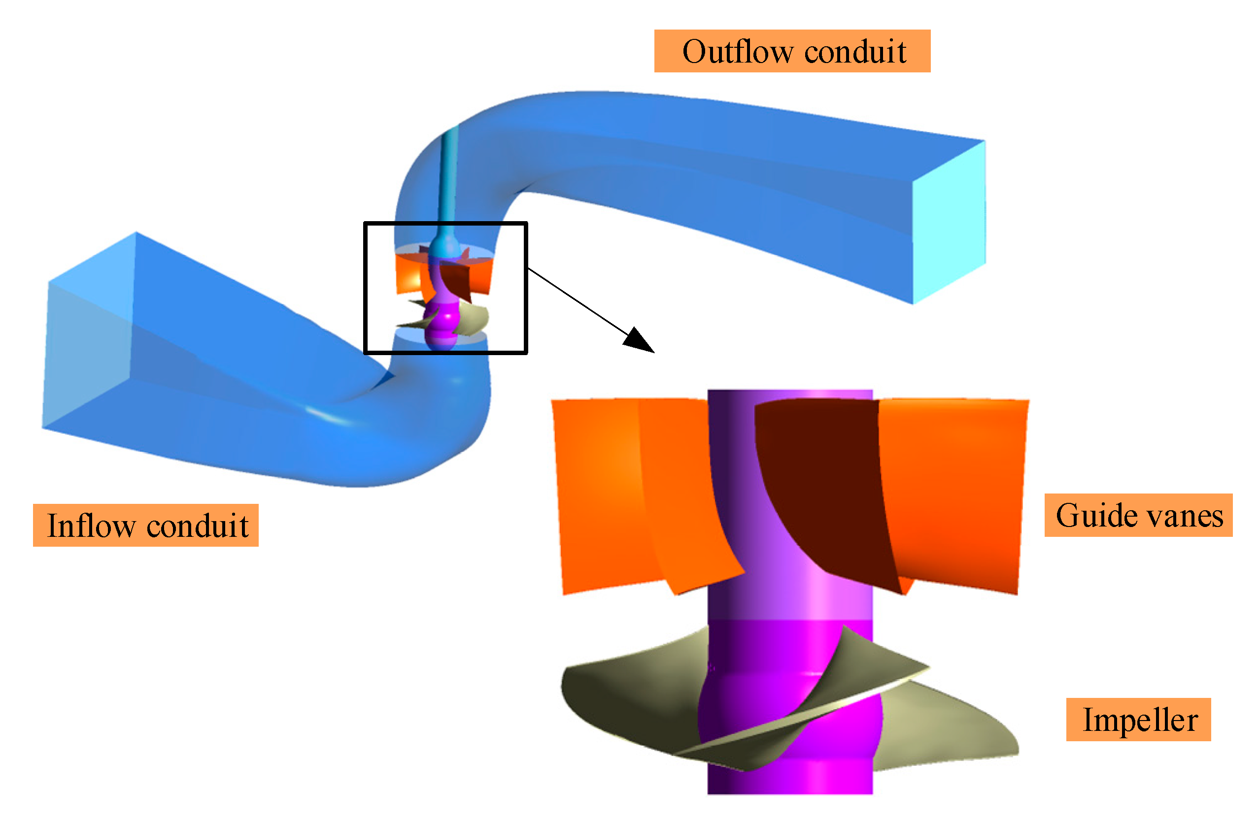
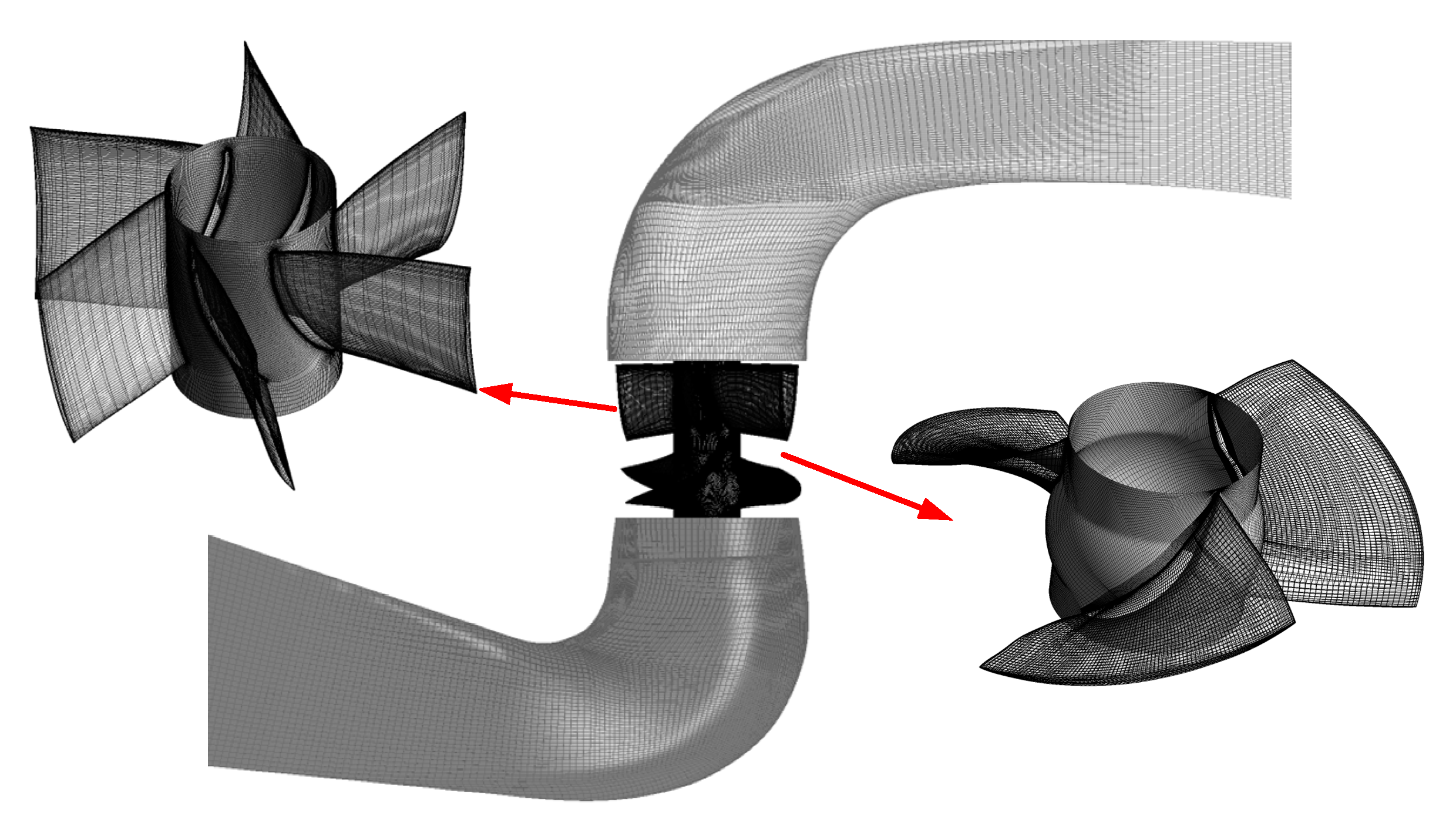
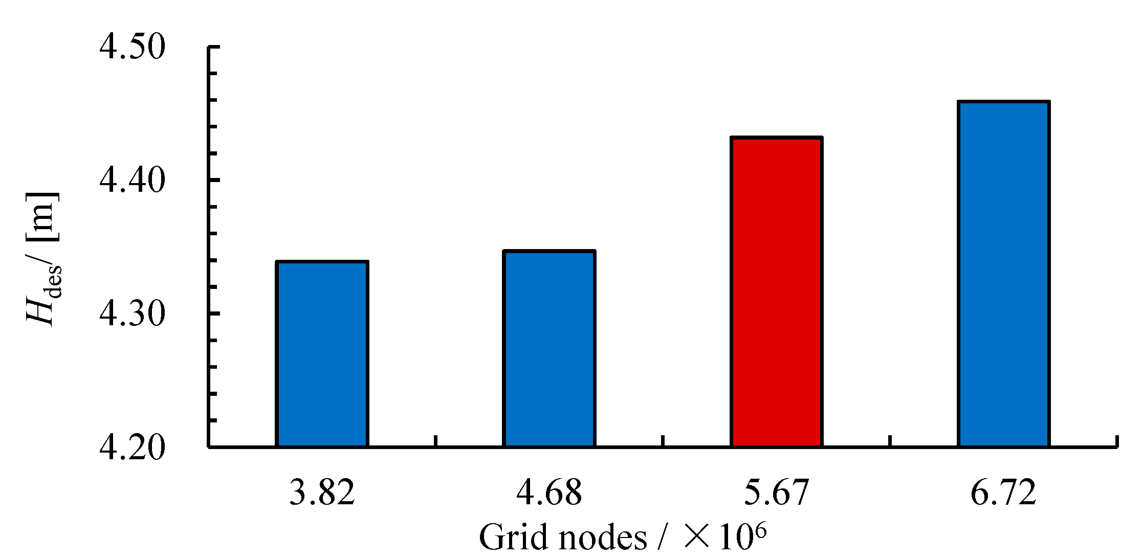
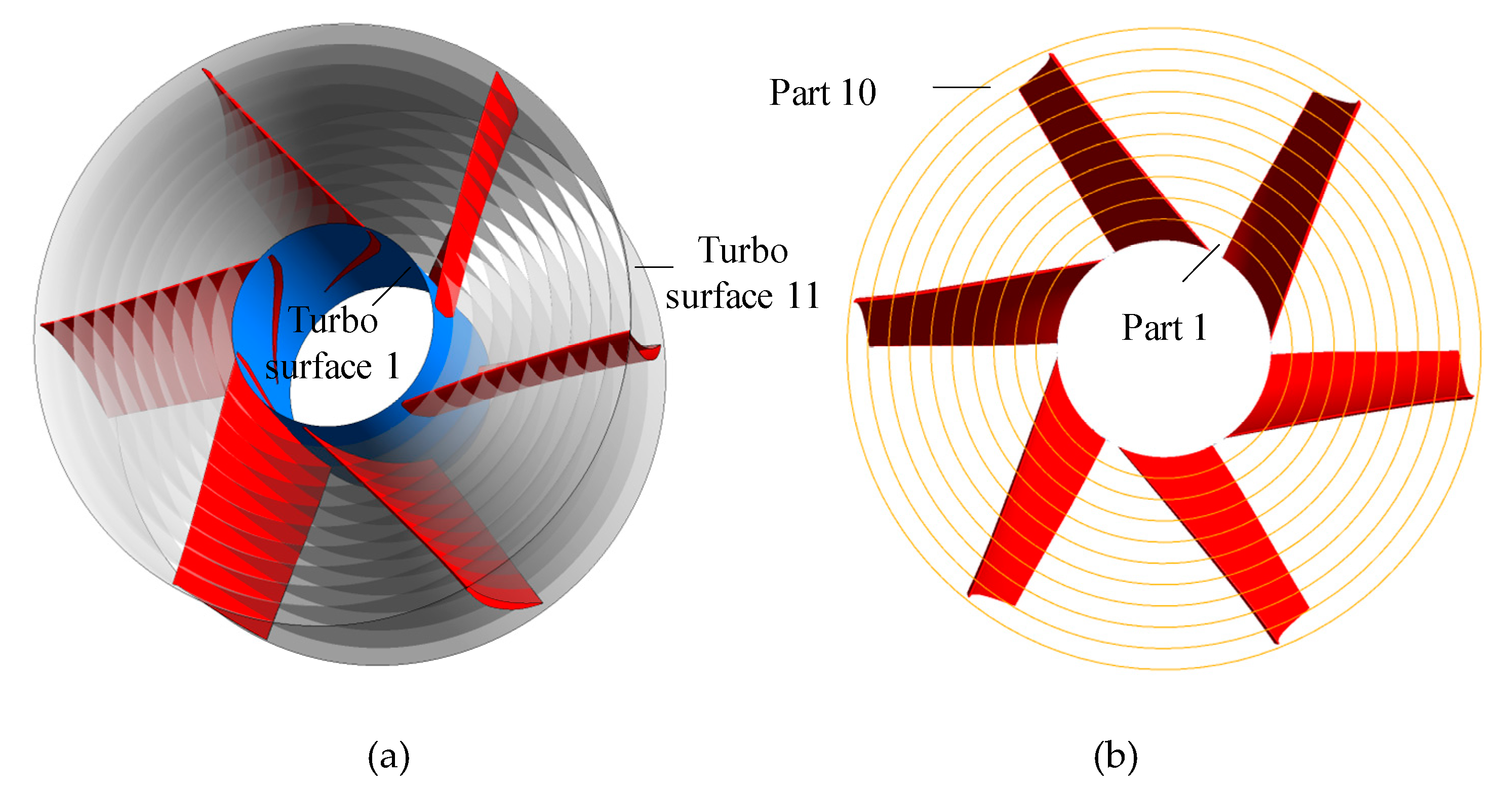
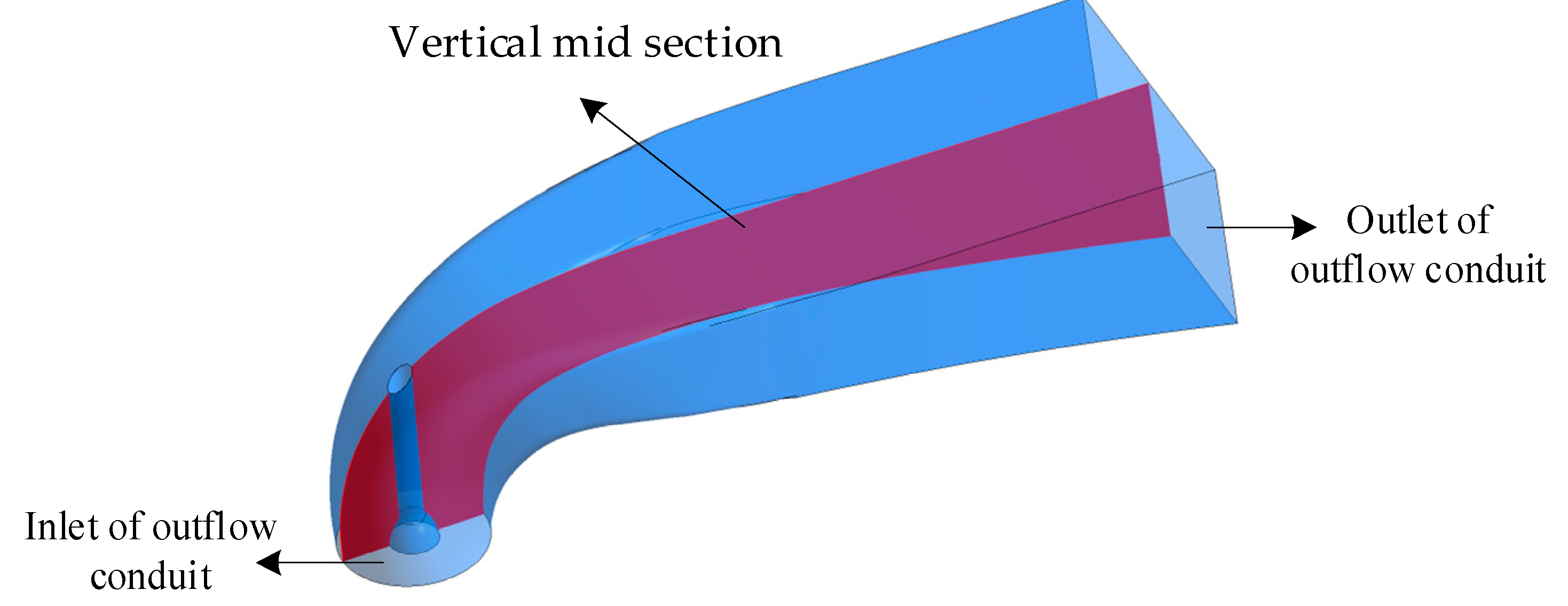
2.1. Three-Dimensional Model and Mesh

A coastal axial-flow pump is divided into inflow conduit, impeller, guide vanes, and outflow conduit as shown in Figure 1. The design head $H_{\mathrm{des}}$, design flow rate $Q_{\mathrm{des}}$, and rotation speed $n$ are 4.4 m, 0.308 m³/s, and 1340 r/min, respectively. The specific speed is 893.4, calculated by $\frac{3.65n{Q}_{\mathrm{des}}{}^{0.5}}{H_{\mathrm{des}}{}^{0.75}}$. The main geometry parameters of impeller and guide vanes are shown in

Table 1. Geometry parameters of impeller and guide vanes.

Parameters	Unit	Value
Impeller
Blade number		3
Impeller diameter	mm	300
Hub diameter	mm	120
Tip clearance radius	mm	0.3
Guide vanes
Vane number		6
Hub dimeter	mm	108
Outlet diameter	mm	325

.

In this work, the hexahedron grids were employed for all calculation domains and the detailed mesh structure can be seen in Figure 2. ICEM CFD was applied to generate the mesh of the inflow conduit, impeller and outflow conduit, while the mesh of guide vanes was produced by TurboGrid. The design head H_des for $\theta$ = 0° was selected as a reference for the mesh refinement as shown in Figure 3. It shows that when the total grid nodes of the coastal axial-flow pump exceed 5,675,561, the relative deviation rate of the design head is less than 0.04%. Therefore, the grid nodes of the inflow conduit, impeller, guide vanes, and outflow conduit were determined as 1,332,635, 1,965,942, 1,226,352, and 1,150,632, respectively. Furthermore, the average Y+ values of the inflow conduit, impeller, guide vanes, and outflow conduit were 5.0, 10.1, 10.8, and 15.9, respectively.

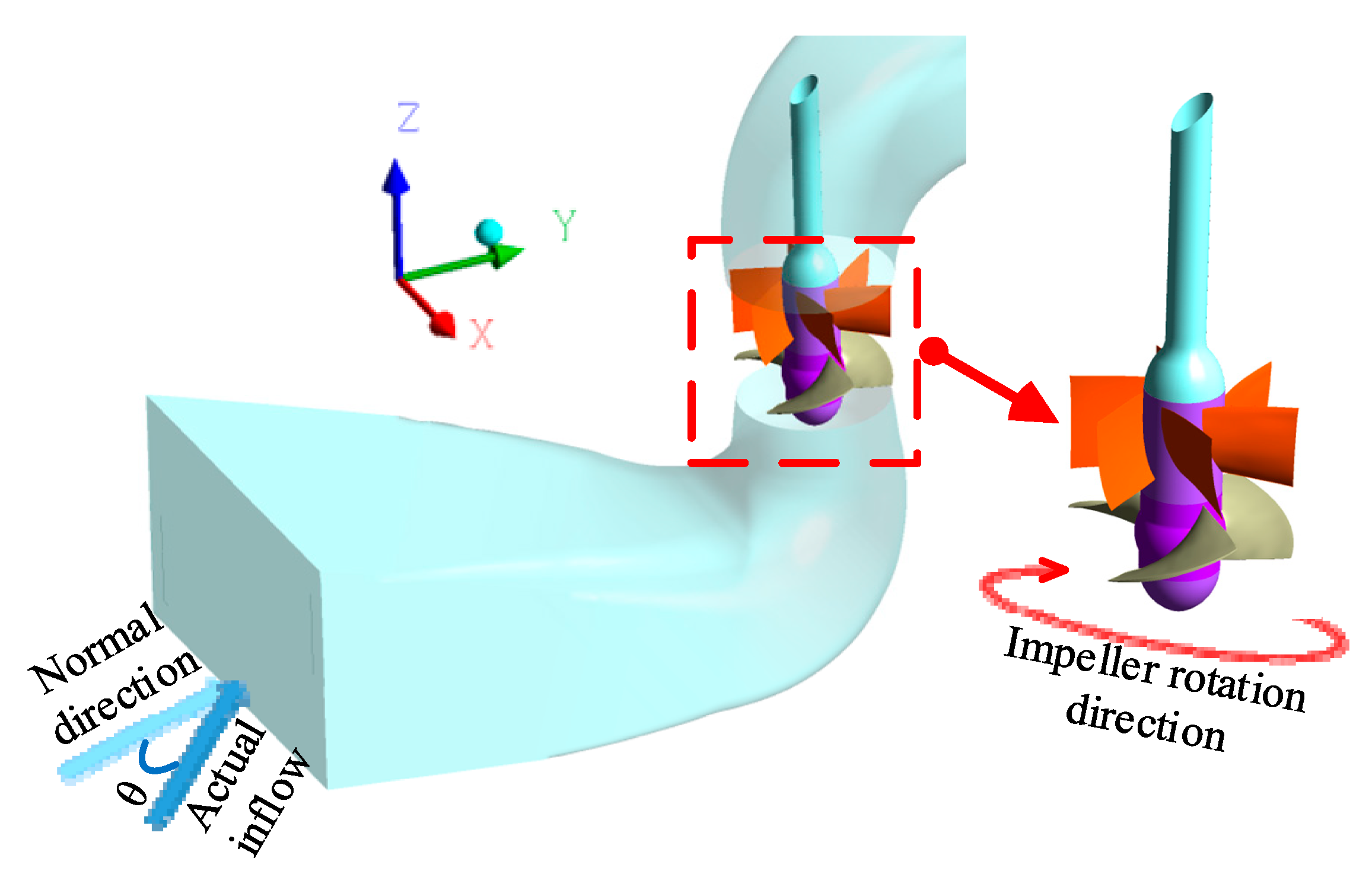
2.2. Governing Equations and Boundary Conditions

In this study, the unsteady Reynolds time-averaged Navier-Stokes equation with an SST k–omega turbulence model was employed to estimate the external characteristic parameters and inner flow field of a coastal axial-flow pump. The steady simulation results were applied as the initial values for the unsteady simulation. The inlet boundary condition was set by velocity inlet. To investigate the effect of inflow distortion, three inflow deflection angles ($\theta$ = 0°, 15°, and 30°) were selected, as shown in Figure 4. The operation flow rate equals actual inflow velocity multiplied by the area of inlet section. The “Opening Pres. And Dirn” was set as outlet boundary condition. The reference pressure and relative pressure were 1 atm and 0 Pa, respectively. The interface condition between guide vanes and outflow conduit was set as “None”. For the steady simulation, the interface conditions between the impeller and stators (inflow conduit and guide vanes) were set as “stage”, which can achieve data transfer between different domains by means of circumferential averaging for the interface. As for the unsteady calculation, the “Transient Rotor Stator” was applied for the interface conditions between the impeller and stators to consider the influence of the relative position of impeller-stator on the internal flow and hydraulic performance, at each time-step. Furthermore, the timestep and total time were 0.000373134 s and 0.447761 s.

2.3. Entropy Production Theory

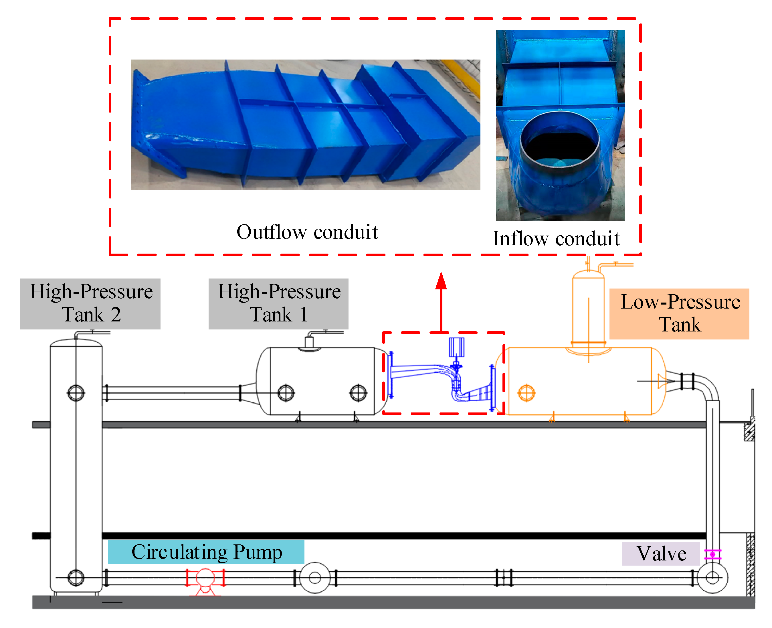
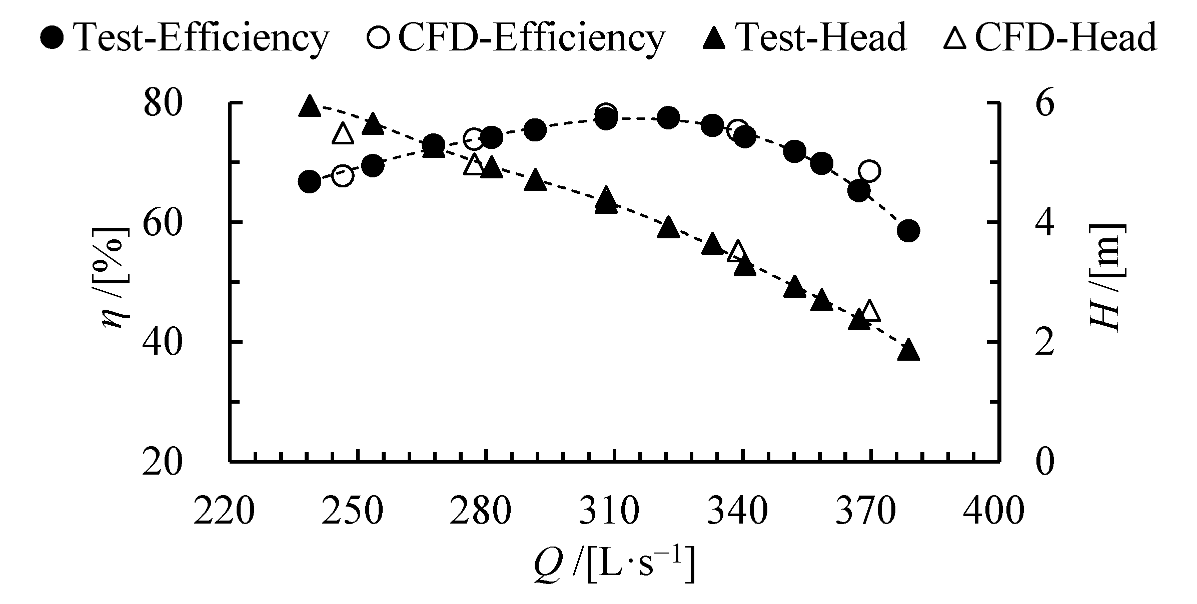
Owing to the presence of viscosity and Reynolds stress in the flow field, part of the mechanical energy of the motor and the total pressure energy in a coastal axial-flow pump will be dissipated as the internal energy (or energy losses) during the pump operation. Entropy, as a parameter of system state, is suitable for describing the internal energy loss. In general, in a coastal axial-flow pump, the flow field is identified as an incompressible and constant temperature. Thus, the entropy production is originated from the dissipation of mechanical energy. Considering that the computational domain is governed by unsteady Reynolds-Averaged Navier–Stokes equations, the entropy production rate caused by the dissipation of mechanical energy $\overline{\left(\frac{\Phi }{T}\right)}$ can be calculated as follows [21,22,23]:

$$\overline{\left(\frac{\Phi }{T}\right)}=S_{{}_{\mathrm{P}\mathrm{R}\mathrm{O}\mathrm{,}\mathrm{D}}}^{\prime }+S_{{}_{\mathrm{P}\mathrm{R}\mathrm{O},\mathrm{I}}}^{\prime }$$

(1)

$$S_{{}_{\mathrm{P}\mathrm{R}\mathrm{O},\mathrm{D}}}^{\prime }=\frac{\mu }{\overline{T}}\left\{2\times \left[{\left(\frac{\partial \overline{u_1}}{\partial x}\right)}^2+{\left(\frac{\partial \overline{u_2}}{\partial y}\right)}^2+{\left(\frac{\partial \overline{u_3}}{\partial z}\right)}^2\right]+{\left(\frac{\partial \overline{u_1}}{\partial y}+\frac{\partial \overline{u_2}}{\partial x}\right)}^2+{\left(\frac{\partial \overline{u_3}}{\partial x}+\frac{\partial \overline{u_1}}{\partial z}\right)}^2+{\left(\frac{\partial \overline{u_2}}{\partial z}+\frac{\partial \overline{u_3}}{\partial y}\right)}^2\right\}$$

(2)

$$S_{{}_{\mathrm{P}\mathrm{R}\mathrm{O},\mathrm{I}}}^{\prime }=\frac{\mu }{\overline{T}}\left\{2\times \left[\overline{{\left(\frac{\partial u_1^{\prime }}{\partial x}\right)}^2}+\overline{{\left(\frac{\partial u_2^{\prime }}{\partial y}\right)}^2}+\overline{{\left(\frac{\partial u_3^{\prime }}{\partial z}\right)}^2}\right]+\overline{{\left(\frac{\partial u_1^{\prime }}{\partial y}+\frac{\partial u_2^{\prime }}{\partial x}\right)}^2}+\overline{{\left(\frac{\partial u_3^{\prime }}{\partial x}+\frac{\partial u_1^{\prime }}{\partial z}\right)}^2}+\overline{{\left(\frac{\partial u_2^{\prime }}{\partial z}+\frac{\partial u_3^{\prime }}{\partial y}\right)}^2}\right\}$$

(3)

where $T$ and $\mu$ are the thermodynamic temperature and dynamic viscosity, respectively. Subscript 1, 2, and 3 stand for the velocity directions of the x, y, and z for the Cartesian coordinate system. $\overline{u}$ and $u^{\prime }$ stands for the time-averaged velocity and velocity fluctuation component. $S_{{}_{\mathrm{P}\mathrm{R}\mathrm{O},\mathrm{D}}}^{\prime }$ represents the entropy production rate originated from the direct dissipation caused by fluid viscous force. $S_{{}_{\mathrm{P}\mathrm{R}\mathrm{O},\mathrm{I}}}^{\prime }$ is the entropy production rate originated from indirect dissipation caused by the velocity fluctuation. $\overline{\left(\frac{\Phi }{T}\right)}$ presents the TEPR.

Solving the unsteady Reynolds-Averaged Navier–Stokes equation cannot obtain the velocity fluctuation components. Therefore, Kock proposed Equation (4) to calculate $S_{{}_{\mathrm{P}\mathrm{R}\mathrm{O},\mathrm{I}}}^{\prime }$ [21,22,23].

$$S_{{}_{\mathrm{P}\mathrm{R}\mathrm{O},\mathrm{I}}}^{\prime }=\frac{\rho \epsilon }{\overline{T}}$$

(4)

where ε is the turbulent dissipation rate.

Finally, the TEP can be estimated as below [21,22,23]:

$$S_{\mathrm{P}\mathrm{R}\mathrm{O},\mathrm{T}}={\displaystyle \underset{V}{\int }(S_{{}_{\mathrm{P}\mathrm{R}\mathrm{O},\mathrm{D}}}^{\prime }+S_{{}_{\mathrm{P}\mathrm{R}\mathrm{O},\mathrm{I}}}^{\prime })dV}$$

(5)

3. Test Validation

In this study, a test for the measurement of the external characteristic parameters in a coastal axial-flow pump was carried out to validate the calculation accuracy and the test bench can be seen in Figure 5. A vertical enclosed structure was applied, which has a two-layer structure. The coastal axial-flow pump, stabilizer tanks, intelligent differential pressure gauges, and torque meters were placed on the upper floor, while electromagnetic flow meters and auxiliary pumps were placed on the lower floor.

Table 2. Main parameters of measuring instrument.

Measurement Instrument	Measurement Items	Maximum Measurement Value	Measurement Uncertainty
Intelligent electromagnetic flowmeter	Flow rate	1800 m3/h	EQ = 0.2%
Intelligent torque and speed sensor	Speed and Torque	200 N·m	EM = 0.1% EN = 0.1%
Intelligent differential pressure transmitter	Head	10 m	EH = 0.1%

presents different main parameters of the measuring instrument. The measurement uncertainties of flow rate and head are E_Q = 0.2% and E_H = 0.1%, respectively. The measurement uncertainties of speed and torque are E_M = 0.1% and E_N = 0.1%, respectively. A less than 0.3% of the system uncertainty of the test bench was determined by $\sqrt{E_Q^2+E_M^2+E_N^2+E_H^2}$.

Figure 6 compares the external characteristic parameters between the CFD results and test data at $\theta$ = 0°. The efficiency curve and head curve of the CFD were similar to that of the test. When $Q\ge 1.0Q_{\mathrm{des}}$, the efficiency and head of CFD were higher than efficiency and head of test, respectively. However, when $Q<1.0Q_{\mathrm{des}}$, the efficiency and head of CFD were slightly lower than efficiency and head of test, respectively. Compared with the efficiency and head of test, the maximum relative errors of the efficiency and head of CFD were less than 5% and 6%, respectively, which verified the reliability of the CFD results.

4. Results and Discussion

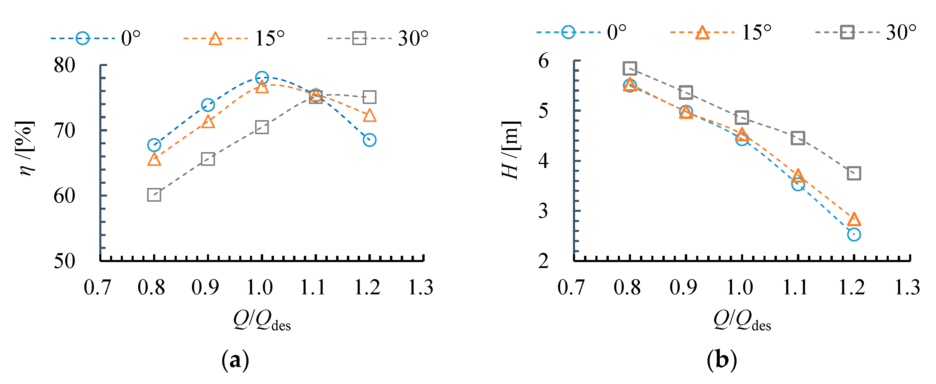
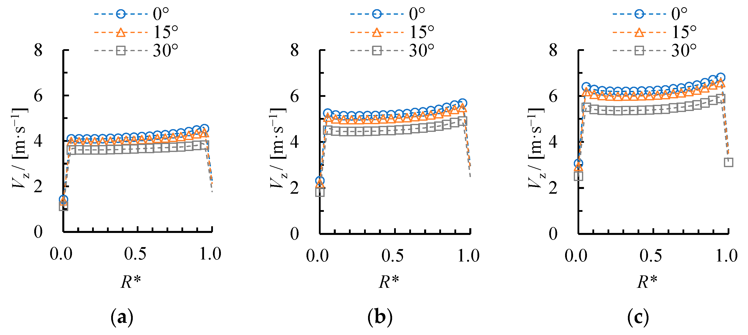
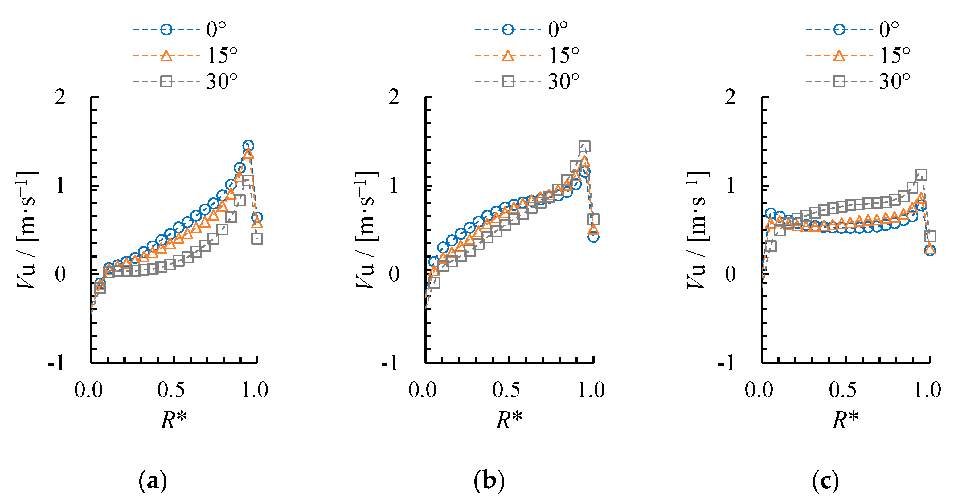
4.1. Pump Performance under Different Inflow Deflection Angles

Figure 7 shows the efficiency and head curves under three $\theta$ values. The pump efficiency decreases with an increase in $\theta$ within Q = 0.8Q_des − 1.1Q_des, but it increases with an increase in $\theta$ within Q = 1.1Q_des − 1.2Q_des. The highest efficiency point shifts to large flow rates as $\theta$ increases. In addition, the pump head declines with an increase in $\theta$.

To clarify the internal relationship between inflow deflection angle, hydraulic performance, and flow pattern at impeller inlet, Figure 8 shows the radial distributions of the axial velocity at impeller inlet under three $\theta$ values. The radial coefficient can be calculated as Equation (6).

$$R^{*}=\frac{R-R_h}{R_{\mathrm{s}}-R_h}$$

(6)

where R_h and R_s denote the hub radius and the shroud radius, respectively. R is the calculated circle radius. The axial velocity first rises and then declines with R* increasing, caused by the wall effect, and it improves with flow rate increase. The axial velocity decreases with $\theta$ increasing, which improves the impeller attack angle. Thus, the highest efficiency point shifts to the larger flow rates and head declines as $\theta$ increases.

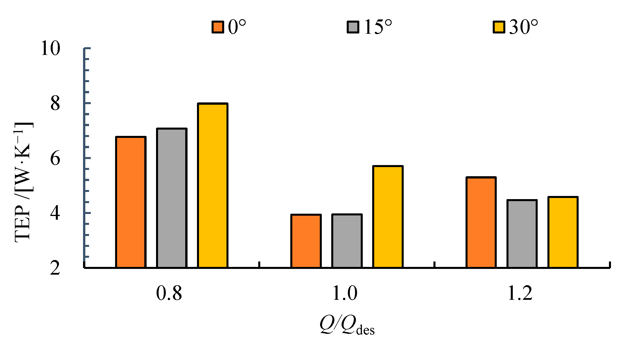
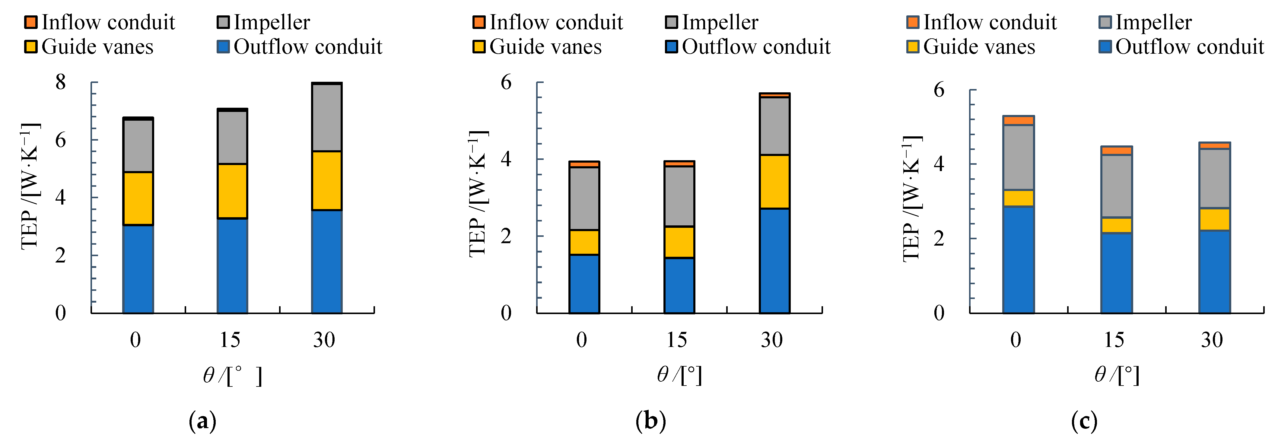
4.2. Distribution of TEP under Different Inflow Deflection Angles

The TEP distribution with three $\theta$ values under different flow rates can be seen in Figure 9. Under 0.8Q_des and 1.0Q_des, TEP increases with an increase in $\theta$. Compared with $\theta$ = 0°, the growth rates of $\theta$ = 30° are 18.0% and 45.1% under 0.8Q_des and 1.0Q_des, respectively. Under 1.2Q_des, TEP first drops and then rises with an increase in $\theta$. Compared with $\theta$ = 0°, the decline rate of $\theta$ = 30° is 13.5%. In addition, the minimum TEP of $\theta$ = 0° and $\theta$ = 15° can be found under 1.0Q_des, and that of $\theta$ = 30° can be found under 1.2Q_des. Under different inflow deflection angles, the flow corresponding to the lowest TEP and the highest efficiency is consistent, which shows that TEP can effectively reflect the impact of the inflow deflection angle on hydraulic performance.

The TEP percentages of the inflow conduit, impeller, guide vanes, and outflow conduit are obtained in the Figure 10. The TEP of the inflow conduit is much lower than that of the impeller, guide vanes, and outflow conduit for each flow rate. Since the circulation of the impeller outflow decreases with the improvement of the flow rate, the TEP proportion of guide vanes declines significantly with the improvement of the flow rate. Under 0.8Q_des, the TEP for the impeller, guide vanes, and outflow conduit increases with $\theta$ increasing. Compared with $\theta$ = 0°, the growth rates with $\theta$ = 30° of the impeller, guide vanes, and outflow conduit are 29.2%, 10.8%, and 16.8%, respectively. Under 1.0Q_des, the influence of $\theta$ on the TEP of the guide vanes and outflow conduit is obvious. Compared with $\theta$ = 0°, the growth rates with $\theta$ = 30° of the guide vanes and outflow conduit are 116.2% and 79.0%, respectively. Under 1.2Q_des, the TEP percentage of the guide vanes is very small, and the TEP of the outflow conduit decreases significantly with an increase in $\theta$. Compared with $\theta$ = 0°, the decline rate with $\theta$ = 30° of the outflow conduit is 22.5%.

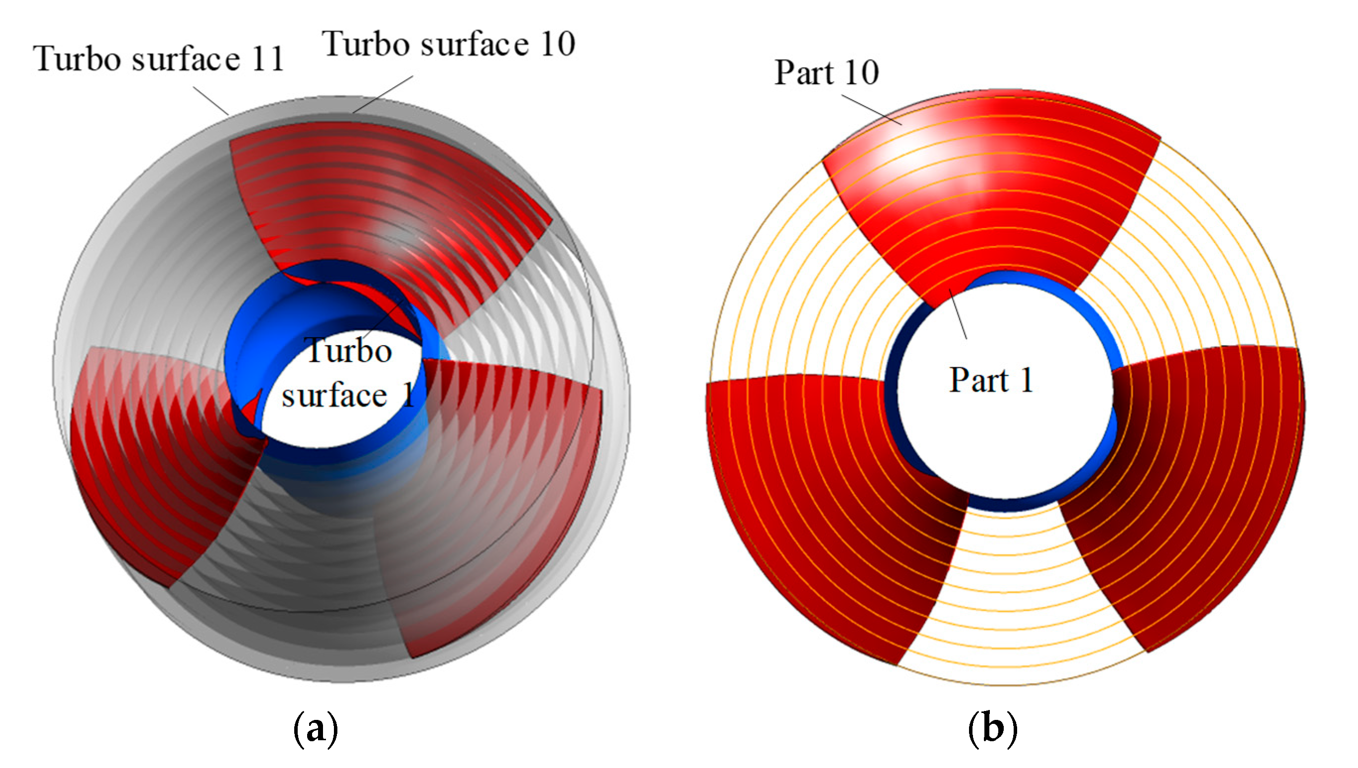
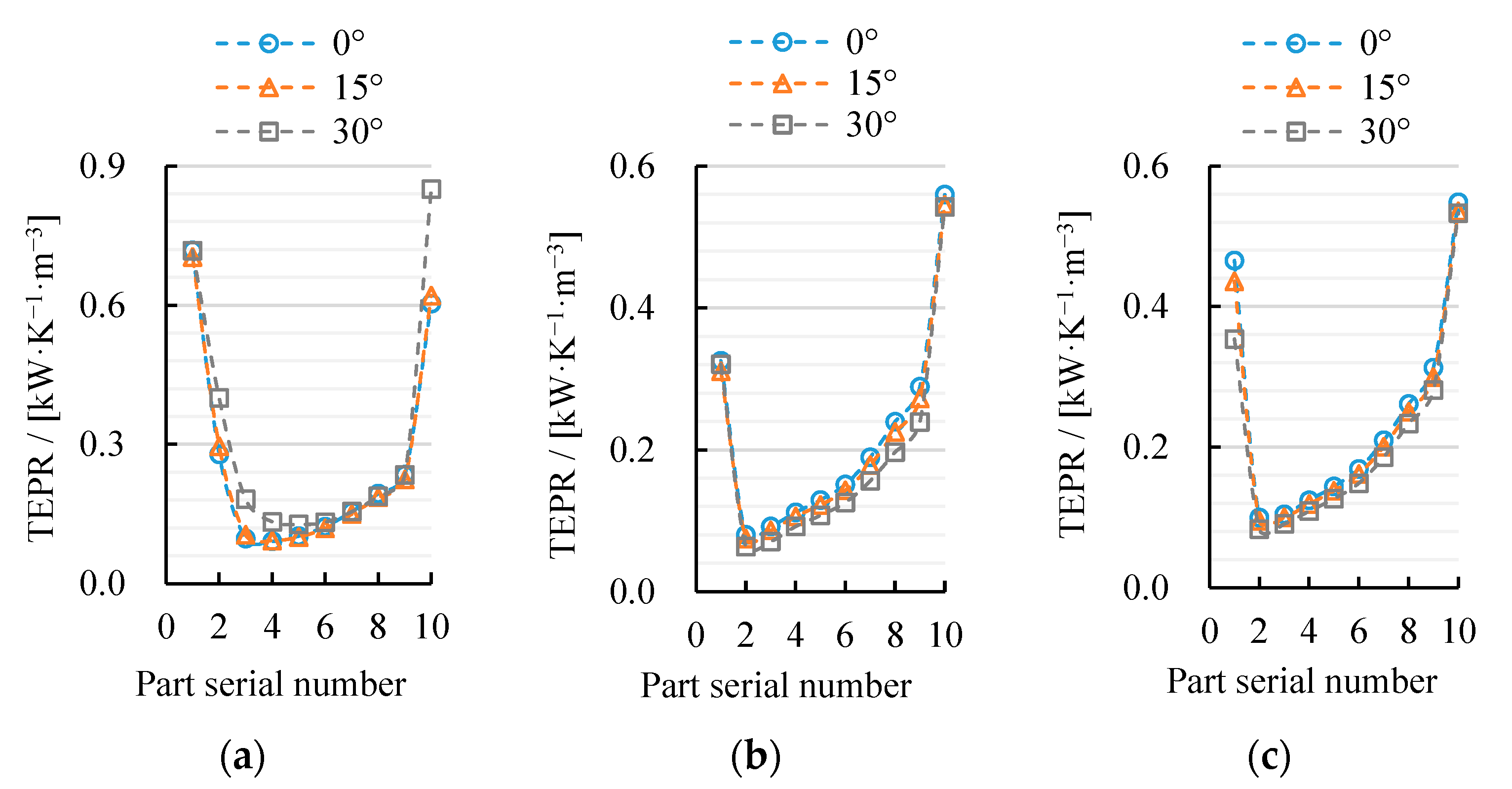
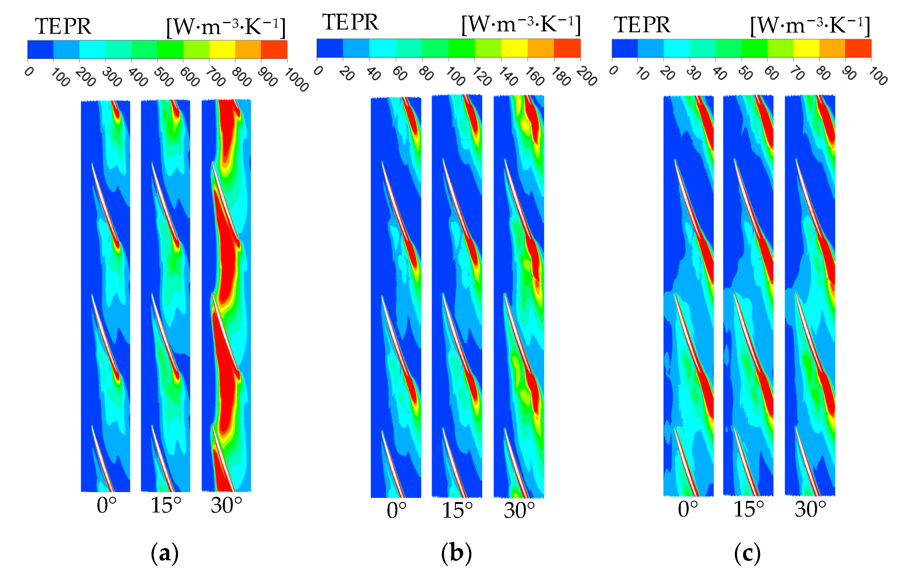
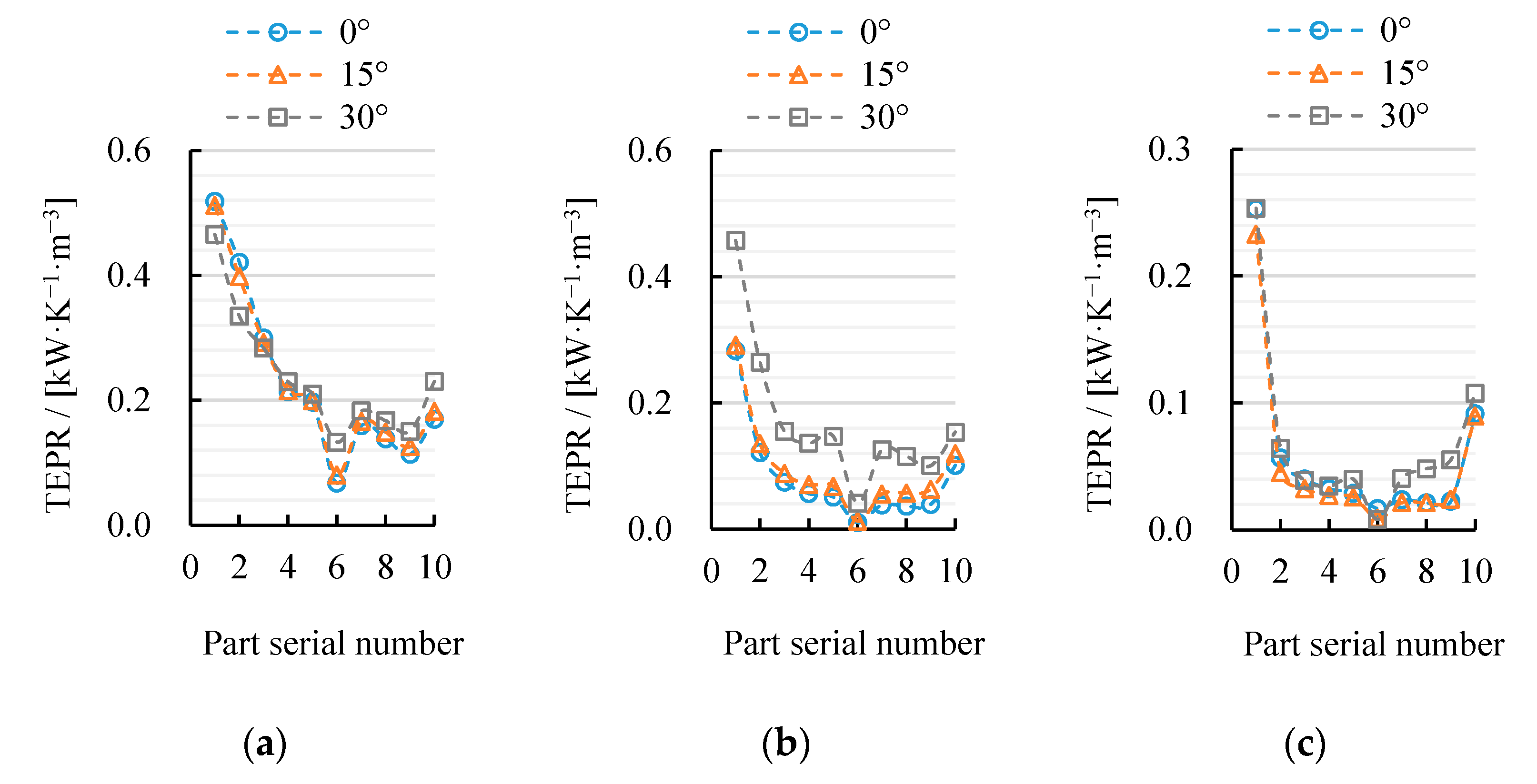
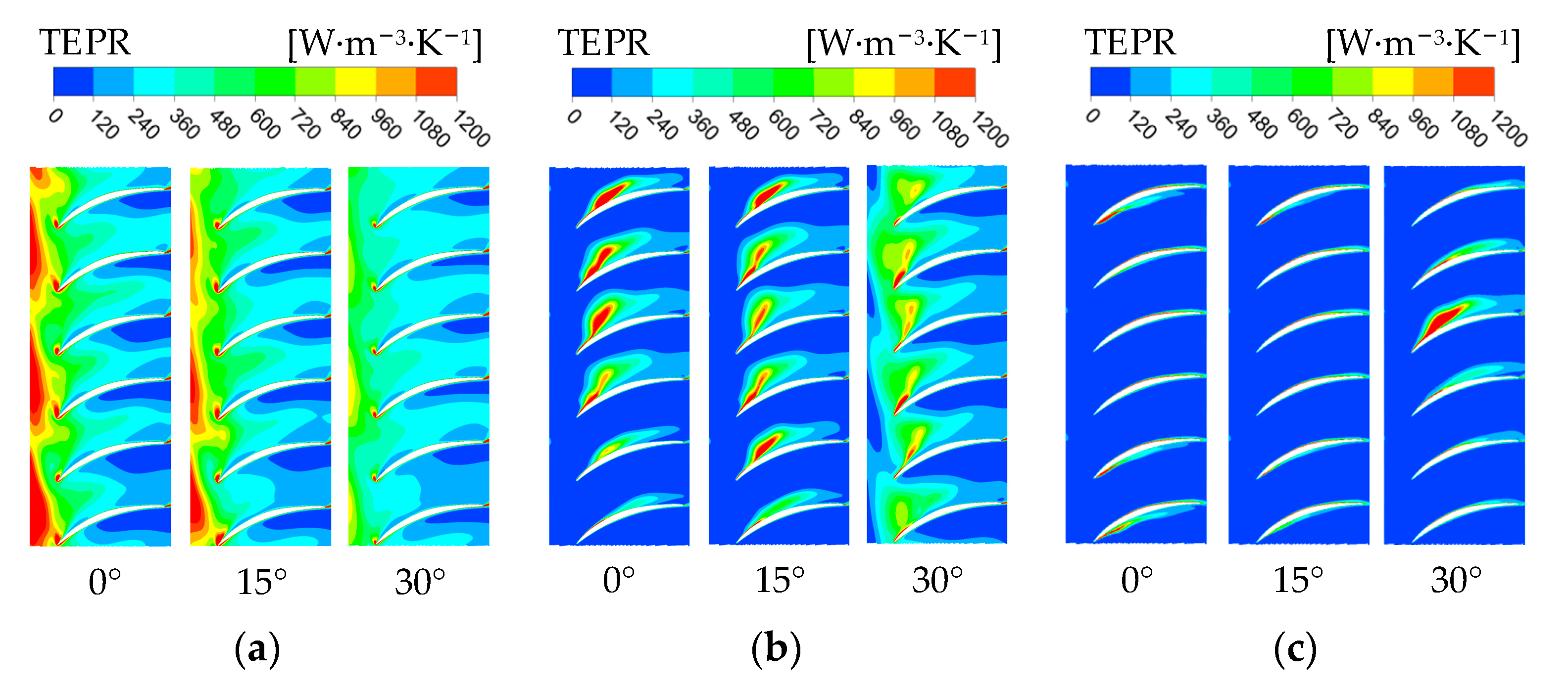
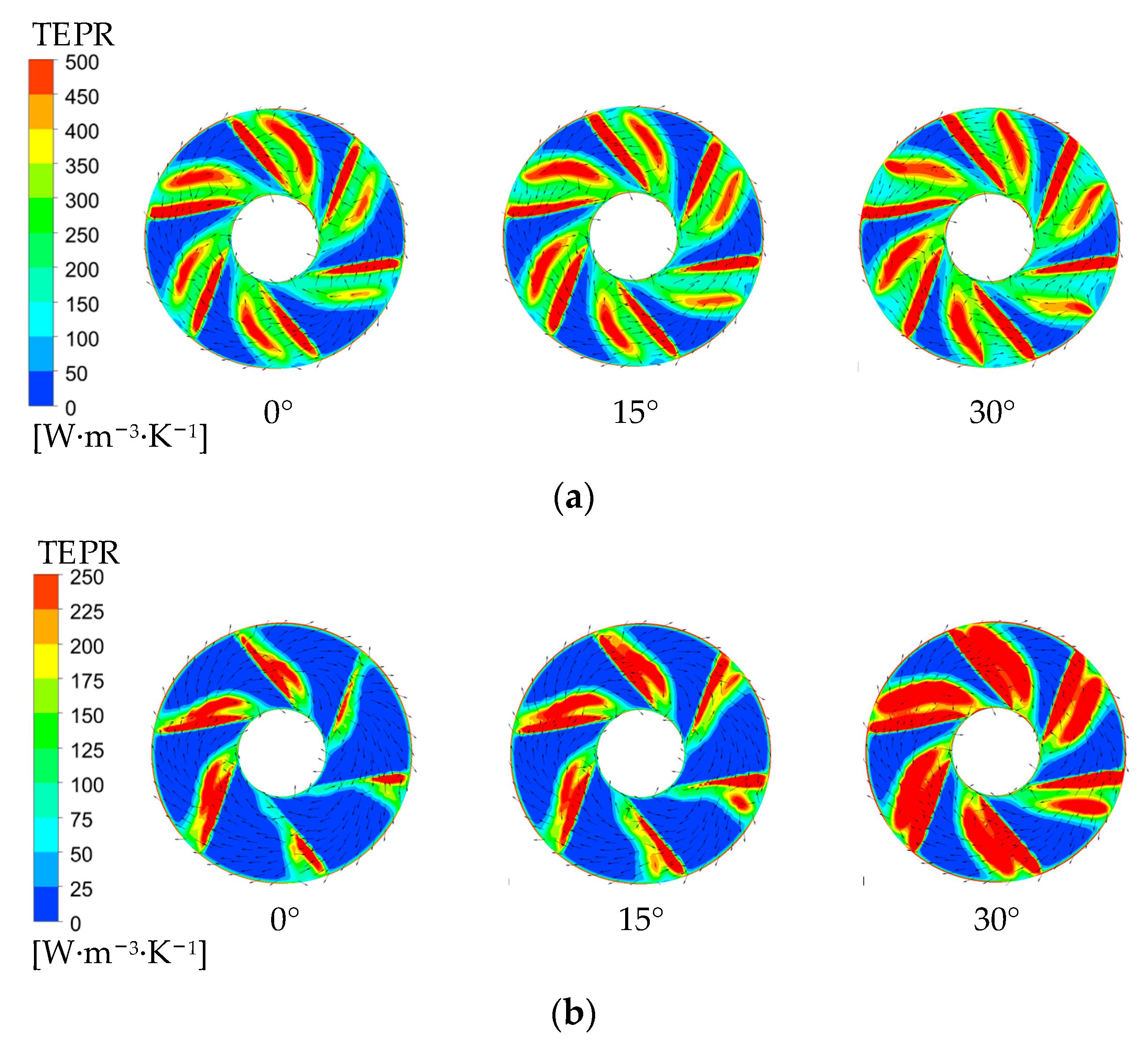
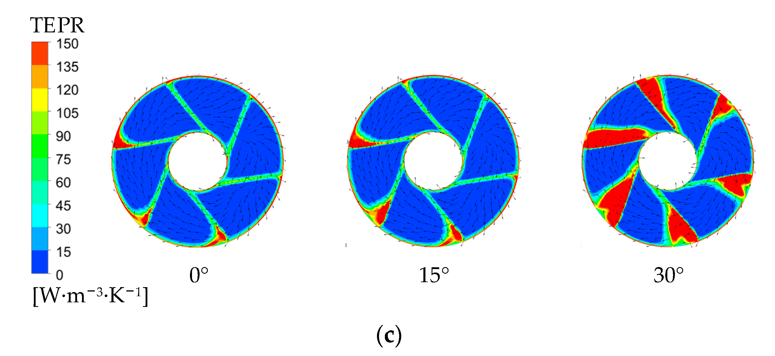
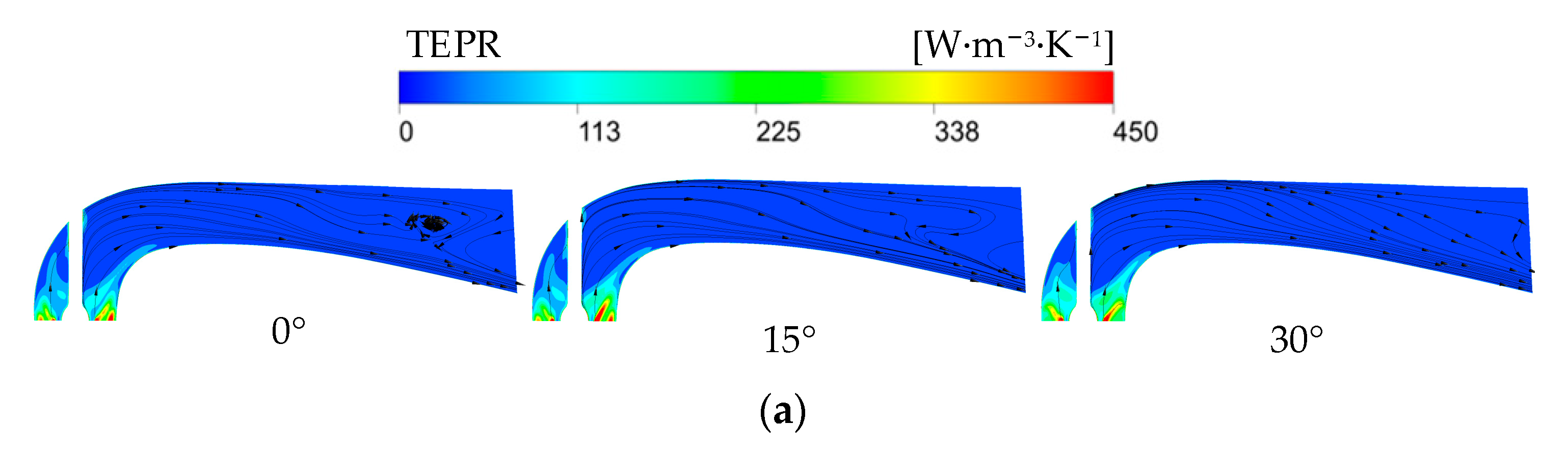
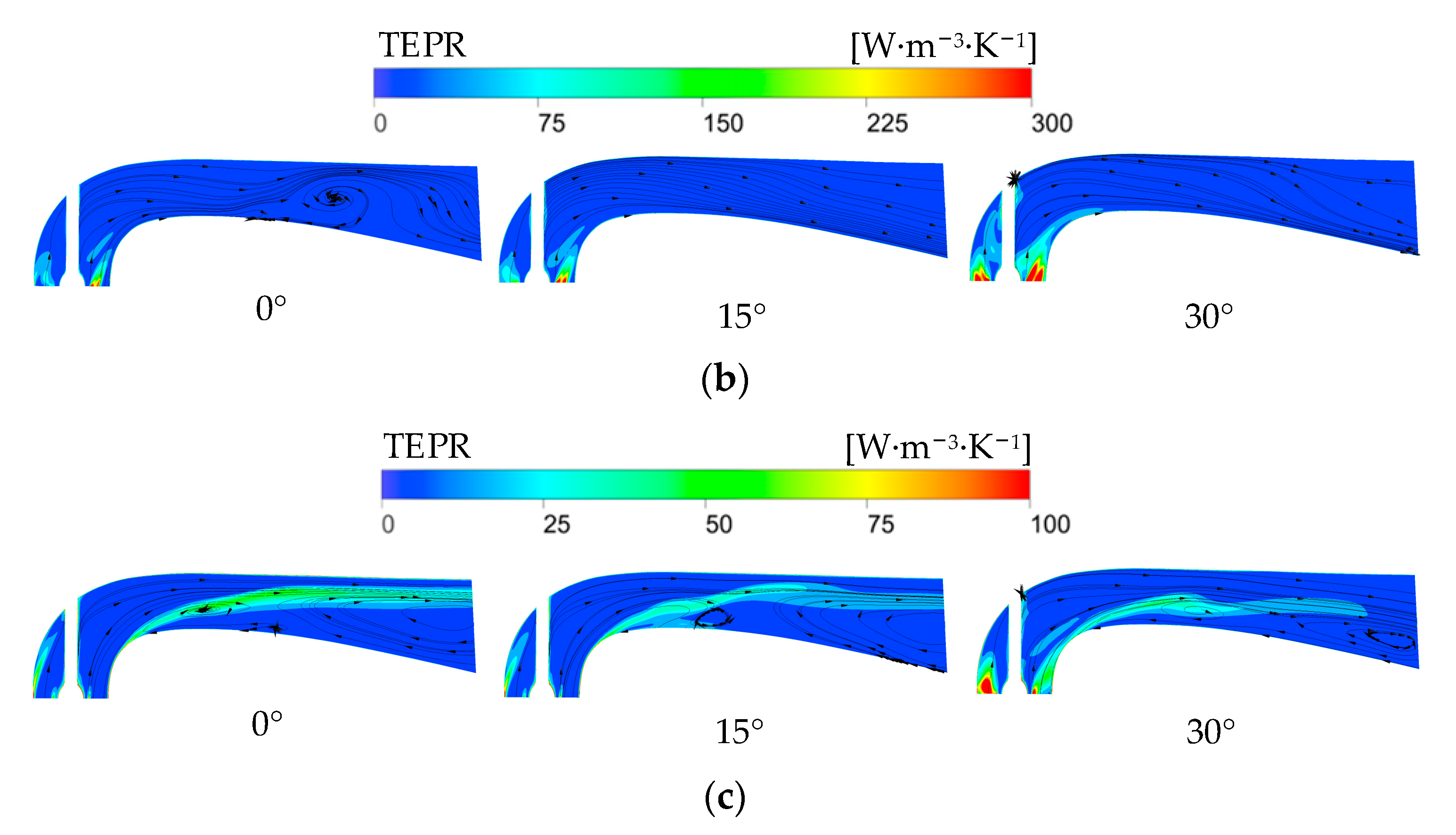
4.3. Distribution of TEPR under Different Inflow Deflection Angles

To obtain the local TEPR in the impeller passage, the impeller passage can be split into 10 parts through 11 turbo surfaces, as can be seen in Figure 11. In this study, R* of turbo surface i was determined by $\left(i-1\right)\times 0.1$. The volume-averaged TEPR of each part in the impeller passage under the three $\theta$ values are found in Figure 12. As a result of the wall effect, the volume-averaged TEPR near hub and shroud is higher than that in other parts. Under 0.8Q_des, the volume-averaged TEPR of Part 2–4 and Part 10 increases obviously with an increase in $\theta$. Compared with $\theta$ = 0°, the relative growth rate of the volume-averaged TEPR of Part 10 with $\theta$ = 30° is 40.8%. Under 1.0Q_des and 1.2Q_des, the volume-averaged TEPR of Part 10 is the largest, caused by tip leakage flow. The volume-averaged TEPR from Part 2 to Part 10 decreases with an increase in $\theta$. Compared with $\theta$ = 0°, the decline rates of the average TEPR of Part 10 with $\theta$ = 30° are 3.1% and 2.8% under 1.0Q_des and 1.2Q_des, respectively.

The TEPR distribution on the turbo surface of impeller passage (R* = 0.95) under three $\theta$ values are obtained in Figure 13. As a result of the decline of attack angle, the flow separation area and TEPR in the vicinity of the suction side decreases with flow rate increasing. The high TEPR near trailing edge can be found caused by the shock effect of the wake vortex on the main stream. In addition, the increase in $\theta$ leads to the enhancement of flow separation and improvement of the high TEPR area in the vicinity of the trailing edge.

The guide vanes passage also can be split into 10 Parts through 11 turbo surfaces to obtain the local TEPR distribution, as can be found in Figure 14. Figure 15 prsents the volume-averaged TEPR in the guide vanes under the three $\theta$. As a result of the wall effect, the volume-averaged TEPR of Part 1 and 10 was obviously higher than that of the other parts. Under 0.8Q_des, the volume-averaged TEPR of Part 6–10 increase with an increase in $\theta$, and the relative increase rate of Part 6 with $\theta$ = 30° is 97.1% compared with $\theta$ = 0°. Under 1.0Q_des, the volume-averaged TEPR of all Part 1–10 increase with an increase in $\theta$, and the relative increase rate of Part 6 with $\theta$ = 30° is 288.5% compared with $\theta$ = 0°. Under 1.2Q_des, the volume average TEPR of Part 7–10 with $\theta$ = 30° is obviously higher than that with $\theta$ = 0°, and the relative increase rate of Part 9 is 143.1%.

Figure 16 shows the local TEPR ditribution on the turbo surface with an R* = 0.1 of the guide vanes. Under 0.8Q_des, there are obvious high TEPRs near the inlet due to the strong impeller-guide vanes interference effect, and high TEPR areas decline with $\theta$ increasing. These results show that an increase in $\theta$ can reduce the impeller-guide vanes interference effect. Under 1.0Q_des, TEPR near the suction side is high originated from flow separation, which shifts to the impeller inlet as $\theta$ increases. Under 1.2Q_des, the fluid flows close to the blade surface, so the high TEPR mainly results from the wall effect of the blade. However, a large area with a high TEPR due to flow separation appears near the suction side when $\theta$ increases to 30°.

The circumferential velocity in the guide vanes outflow has a significant influence on the hydraulic losses in the outflow conduit. Figure 17 denotes the radial distribution of the circumferential velocity located in the guide vanes outlet under three $\theta$ values. Under 0.8Q_des, the circumferential velocity increases from R* = 0 to R* = 0.9, but it decreases from R* = 0.9 to R* = 1.0, originated from the wall effect. The secondary vortex in the outlet section is enhanced by an increase in $\theta$, which results in a block effect and a decline in circumferential velocity. Therefore, the circumferential velocity drops with $\theta$ increasing. Under 1.0Q_des, the circumferential velocity increases from R* = 0 to R* = 0.9, and it decreases from R* = 0.9 to R* = 1.0, respectively. The circumferential velocity increases with an increase in $\theta$ within R* = 0.8–1.0, which indicates that obvious secondary vortex structure near the shroud cannot be found. Under 1.2Q_des, the circumferential velocity increases with an increase in $\theta$ within R* = 0.4–1.0. This phenomenon shows that there is no obvious secondary vortex structure at outlet.

Figure 18 shows the local TEPR distribution in the inlet of the outflow conduit under the three $\theta$ values. Due to the shock effect of secondary vortices on the main stream, there are obviously high TEPR at the inlet, and the positions of these TEPR correspond to the positions of the guide vanes. Furthermore, the high TEPR area drops with flow rate increasing, which indicates that the block effect of secondary vortices declines with flow rate increasing. However, the high TEPR area increases with an increase in $\theta$, which indicates that the intensity of secondary vortices increases with an increase in $\theta$.

The position of vertical mid section of the outflow conduit is shown in Figure 19. Figure 20 depicts the local TEPR distribution and velocity vector in the vertical mid section of the outflow conduit. Due to the influence of residual circulation in the outflow of the guide vanes, high TEPR can be found in the vicinity of the inlet of the outflow conduit with a decrease in TEPR along the direction of inlet to outlet. For 0.8Q_des, the high TEPR area near the inlet improves with $\theta$ rising, resulting from the enhancement of the secondary vortex strength. When the internal fluid passes the corner of the outflow conduit, the flow direction changes, which results in a reverse pressure gradient and a backflow near the outlet. Consequently, the intensity of the vortex structure decreases with an increase in $\theta$. Under 1.0Q_des, the TEPR and backflow intensity decreases, compared with 0.8Q_des. However, the high TEPR area near the inlet increases and the backflow area near outlet declines, as $\theta$ increases. Under 1.2Q_des, TEPR decreases further, but the backflow intensity increases significantly, compared with 0.8Q_des. There is an obvious high TEPR downstream of the corner caused by a large backflow. As the inflow deflection angle increases, the area with a high TEPR near the inlet and downstream of the corner increases and declines with an increase in $\theta$.

5. Conclusions

In this work, the unsteady Reynolds-Averaged Navier–Stokes equation with SST k–omega turbulence model was solved to predict the external characteristic parameters and the unsteady flow field in a coastal axial for three different inflow deflection angles. The effect of the various inflow deflection angles on the hydraulic losses was investigated using the entropy production theory. The main findings were concluded as below:

(1) The axial velocity at the impeller inlet decreases as $\theta$ increases, which results in an improvement in the attack angle. Therefore, the head decreases and the highest efficiency point shifts to large flow rate, as $\theta$ increases. Moreover, the TEP of the coastal axial-flow pump increases with an increase in $\theta$ under 0.8Q_des and 1.0Q_des, but the TEP of the coastal axial-flow pump with $\theta$ = 0° is obviously higher than that with $\theta$ = 15° and 30° under 1.2Q_des.

(2) The TEP inside the impeller increases with an increase in $\theta$ under 0.8Q_des, but it decreases with an increase in $\theta$ under 1.0Q_des and 1.2Q_des. The TEPR near the hub and the shroud is high, originated from the wall effect and tip leakage flow. The high TEPR area near the trail edge rises with $\theta$ increasing.

(3) The TEP inside the guide vanes with $\theta$ = 30° is obviously higher than that with $\theta$ = 0° and 15°. The highest TEPR can be obviously found near the hub. The high TEPR area at the leading edge near the hub decreases with an increase in $\theta$. When $\theta$ increases to 30°, there is a high TEPR near the suction surface under 1.2Q_des.

(4) Under 0.8Q_des and 1.0Q_des, the increase in the inflow deflection angle enhances the strength of the secondary vortex at the inlet of the outflow conduit and the barrier effect, leading to an obvious increase for the TEP inside the outflow conduit with $\theta$ = 30° compared to that with $\theta$ = 0° and 15°.

These results can provide corrective suggestions for theoretical hydraulic design, so that the coastal axial-flow pump can be better applied in practical engineering.

References

1. Xie, C.; Tang, F.; Liu, C.; Yang, F. Model test analysis of impeller selection in large vertical axial flow pumping system. Trans. Chin. Soc. Agric. Mach. 2017, 48, 94–99+131. [Google Scholar]
2. Yang, F.; Zhao, H.; Liu, C.; He, J.; Tang, F. Experiment and analysis on outlet flow pattern and pressure fluctuation in inlet conduit of vertical axial-flow pumping system. Trans. Chin. Soc. Agric. Mach. 2017, 48, 141–146+113. [Google Scholar]
3. Liu, C.; Liang, H.; Yan, J.; Yang, F.; Chen, F.; Yang, H. PIV measurements of intake flow field in axial-flow pump. Trans. Chin. Soc. Agric. Mach. 2015, 46, 33–41. [Google Scholar]
4. Peng, G.; Chen, Q.; Zhou, L.; Pan, B.; Zhu, Y. Effect of blade outlet angle on the flow field and preventing overload in a centrifugal pump. Micromachines 2020, 11, 811. [Google Scholar] [CrossRef]
5. Li, J.; Tang, L.; Zhang, Y. The influence of blade angle on the performance of plastic centrifugal pump. Adv. Mater. Sci. Eng. 2020, 2020, 7205717. [Google Scholar] [CrossRef]
6. Han, W.; Zhang, T.; Su, Y.L.; Chen, R.; Qiang, Y.; Han, Y. Transient Characteristics of Water-Jet Propulsion with a Screw Mixed Pump during the Startup Process. Math. Probl. Eng. 2020, 2020, 5691632. [Google Scholar] [CrossRef]
7. Wei, Q.; Sun, X.; Asaad, Y.S.; Li, C. Impacts of blade inlet angle of diffuser on the performance of a submersible pump. Proc. Inst. Mech. Eng. Part E J. Process Mech. Eng. 2020, 234, 613–623. [Google Scholar]
8. Chen, J.; Shi, W.; Zhang, D. Influence of blade inlet angle on the performance of a single blade centrifugal pump. Eng. Appl. Comput. Fluid Mech. 2021, 15, 462–475. [Google Scholar] [CrossRef]
9. Wang, W.; Tai, G.; Pei, J.; Pavesi, G.; Yuan, S. Numerical investigation of the effect of the closure law of wicket gates on the transient characteristics of pump-turbine in pump mode. Renew. Energy 2022, 194, 719–733. [Google Scholar] [CrossRef]
10. Kan, N.; Liu, Z.; Shi, G.; Liu, X. Effect of Tip Clearance on Helico-Axial Flow Pump Performance at Off-Design Case. Processes 2021, 9, 1653. [Google Scholar] [CrossRef]
11. Cheng, H.; Li, H.; Yin, J.; Gu, X.; Hu, Y.; Wang, D. Investigation of the distortion suction flow on the performance of the canned nuclear coolant pump. In Proceedings of the 2014 ISFMFE-6th International Symposium on Fluid Machinery and Fluid Engineering, Wuhan, China, 22–25 October 2014; pp. 1–6. [Google Scholar]
12. Zhao, G.; Liang, N.; Zhang, Y.; Cao, L.; Wu, D. Dynamic behaviors of blade cavitation in a water jet pump with inlet guide vanes: Effects of inflow non-uniformity and unsteadiness. Appl. Ocean. Res. 2021, 117, 102889. [Google Scholar] [CrossRef]
13. Zheng, Y.; Li, Y.; Zhu, X.; Sun, D.; Meng, F. Influence of asymmetric inflow on the transient pressure fluctuation characteristics of a vertical mixed-flow pump. Proc. Inst. Mech. Eng. Part A J. Power Energy 2022, 09576509221096926. [Google Scholar] [CrossRef]
14. Long, Y.; Dezhong, W.; Yin, J.; Hu, Y.; Ran, H. Numerical investigation on the unsteady characteristics of reactor coolant pumps with non-uniform inflow. Nucl. Eng. Des. 2017, 320, 65–76. [Google Scholar]
15. Wang, Y.; Wang, P.; Tan, X.; Xu, Z.; Ruan, X. Research on the non-uniform inflow characteristics of the canned nuclear coolant pump. Ann. Nucl. Energy 2018, 115, 423–429. [Google Scholar] [CrossRef]
16. Xu, R.; Long, Y.; Wang, D. Effects of rotating speed on the unsteady pressure pulsation of reactor coolant pumps with steam-generator simulator. Nucl. Eng. Des. 2018, 333, 25–44. [Google Scholar] [CrossRef]
17. Wang, Y.; Xu, Z.; Wang, P.; Wang, J.; Ruan, X. Numerical and experimental analysis on the non-uniform inflow characteristics of a reactor coolant pump with a steam generator channel head. Eng. Appl. Comput. Fluid Mech. 2020, 14, 477–490. [Google Scholar]
18. Cao, P.; Wang, Y.; Kang, C.; Li, G.; Zhang, X. Investigation of the role of non-uniform suction flow in the performance of water-jet pump. Ocean. Eng. 2017, 140, 258–269. [Google Scholar] [CrossRef]
19. Cao, P.; Zhu, R. Prediction and Evaluation of Waterjet Pump Performance under Nonuniform Inflow Using Parallel Compressor Theory. Water 2021, 13, 99. [Google Scholar] [CrossRef]
20. Luo, X.; Ye, W.; Huang, R.; Wang, Y.; Du, T.; Huang, C. Numerical investigations of the energy performance and pressure fluctuations for a waterjet pump in a non-uniform inflow. Renew. Energy 2020, 153, 1042–1052. [Google Scholar] [CrossRef]
21. Kock, F.; Herwig, H. Local entropy production in turbulent shear flows: A high-Reynolds number model with wall functions. Int. J. Heat Mass Transf. 2004, 47, 2205–2215. [Google Scholar] [CrossRef]
22. Herwig, H.; Kock, F. Direct and indirect methods of calculating entropy generation rates in turbulent convective heat transfer problems. Heat Mass Transf. 2007, 43, 207–215. [Google Scholar] [CrossRef]
23. Kock, F.; Herwig, H. Entropy production calculation for turbulent shear flows and their implementation in CFD codes. Int. J. Heat Fluid Flow 2005, 26, 672–680. [Google Scholar] [CrossRef]
24. Shen, S.; Qian, Z.; Ji, B. Numerical analysis of mechanical energy dissipation for an axial-flow pump based on entropy generation theory. Energies 2019, 12, 4162. [Google Scholar] [CrossRef]
25. Wang, L.; Lu, J.; Liao, W.; Guo, P.; Feng, J.; Luo, X.; Wang, W. Numerical investigation of the effect of T-shaped blade on the energy performance improvement of a semi-open centrifugal pump. J. Hydrodyn. 2021, 33, 736–746. [Google Scholar] [CrossRef]
26. Ji, L.; Li, W.; Shi, W.; Tian, F.; Agarwal, R. Diagnosis of internal energy characteristics of mixed-flow pump within stall region based on entropy production analysis model. Int. Commun. Heat Mass Transf. 2020, 117, 104784. [Google Scholar] [CrossRef]
27. Fei, Z.; Zhang, R.; Xu, H.; Feng, J.; Mu, T.; Chen, Y. Energy performance and flow characteristics of a slanted axial-flow pump under cavitation conditions. Phys. Fluids 2022, 34, 035121. [Google Scholar] [CrossRef]
Figure 1. Geometry structure of a coastal axial-flow pump.
Jmse 10 01283 g001
Figure 2. Mesh of the coastal axial-flow pump.
Jmse 10 01283 g002
Figure 3. Grid independence analysis.
Jmse 10 01283 g003
Figure 4. Definition of the inflow deflection angle.
Jmse 10 01283 g004
Figure 5. Test bench photo.
Jmse 10 01283 g005
Figure 6. The external characteristic parameters of CFD and test at θ = 0°.
Jmse 10 01283 g006
Figure 7. The (a) efficiency and (b) head curves under three inflow deflection angles.
Jmse 10 01283 g007
Figure 8. The axial velocity at the impeller inlet with three inflow deflection angles under (a) 0.8Qdes, (b) 1.0Qdes, and (c) 1.2Qdes.
Jmse 10 01283 g008
Figure 9. TEP distribution with three inflow deflection angles under 0.8Qdes, 1.0Qdes, and 1.2Qdes.
Jmse 10 01283 g009
Figure 10. TEP percentage of hydraulic components with three inflow deflection angles under (a) 0.8Qdes, (b) 1.0Qdes, and (c) 1.2Qdes.
Jmse 10 01283 g010
Figure 11. The division diagram of (a) turbo surface and (b) part of impeller.
Jmse 10 01283 g011
Figure 12. The volume-averaged TEPR in the impeller with three inflow deflection angles under (a) 0.8Qdes, (b) 1.0Qdes, and (c) 1.2Qdes.
Jmse 10 01283 g012
Figure 13. The TEPR distribution on the turbo surface of the impeller with three inflow deflection angles under (a) 0.8Qdes, (b) 1.0Qdes, and (c) 1.2Qdes. (R* = 0.95).
Jmse 10 01283 g013
Figure 14. The division diagram of (a) turbo surface and (b) part of guide vanes.
Jmse 10 01283 g014
Figure 15. The volume-averaged TEPR in the guide vanes with three inflow deflection angles under (a) 0.8Qdes, (b) 1.0Qdes, and (c) 1.2Qdes.
Jmse 10 01283 g015
Figure 16. The TEPR distribution on the turbo surface of the guide vanes with three inflow deflection angles under (a) 0.8Qdes, (b) 1.0Qdes, and (c) 1.2Qdes. (R* = 0.1).
Jmse 10 01283 g016
Figure 17. The radial distribution of the circumferential velocity of the guide vanes outlet under (a) 0.8Qdes, (b) 1.0Qdes, and (c) 1.2Qdes.
Jmse 10 01283 g017
Figure 18. TEPR distribution in the outlet of guide vanes with three inflow deflection angles under (a) 0.8Qdes, (b) 1.0Qdes, and (c) 1.2Qdes.
Jmse 10 01283 g018aJmse 10 01283 g018b
Figure 19. The position of vertical mid section of the outflow conduit.
Jmse 10 01283 g019
Figure 20. The TEPR distibution and velocity vector in the vertical mid section of the outflow conduit with three inflow deflection angles under (a) 0.8Qdes, (b) 1.0Qdes, and (c) 1.2Qdes.
Jmse 10 01283 g020aJmse 10 01283 g020b