
Empirical Failure Pressure Prediction Equations for Pipelines with Longitudinal Interacting Corrosion Defects Based on Artificial Neural Network


Abstract
:1. Introduction
- Development of failure pressure assessment method for medium- to high-toughness pipeline with longitudinally aligned interacting corrosion defects subjected to internal pressure and axial compressive stress.
- Establishment of a correlation between defect geometry, axial compressive stress, and failure pressure of a medium- to high-toughness pipeline with longitudinally aligned interacting corrosion defects subjected to internal pressure and axial compressive stress.
2. Methodology
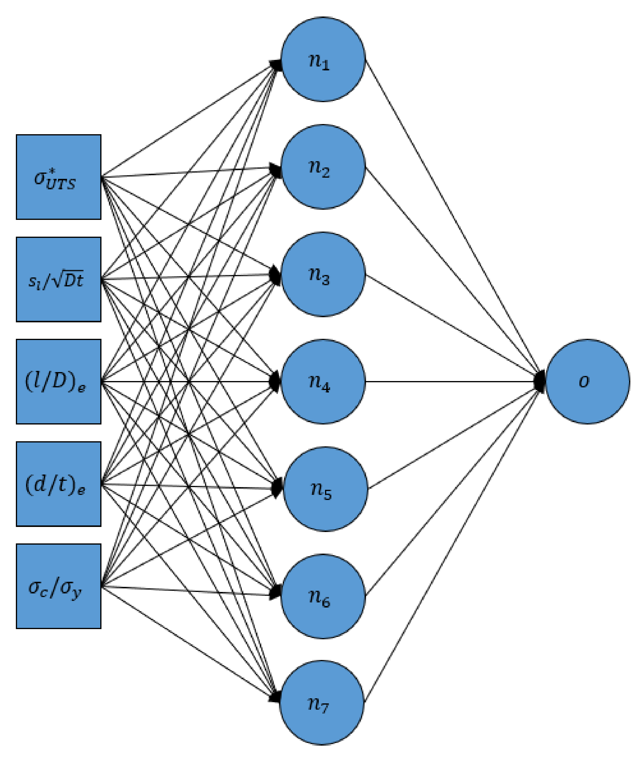
2.1. Development of the Artificial Neural Network
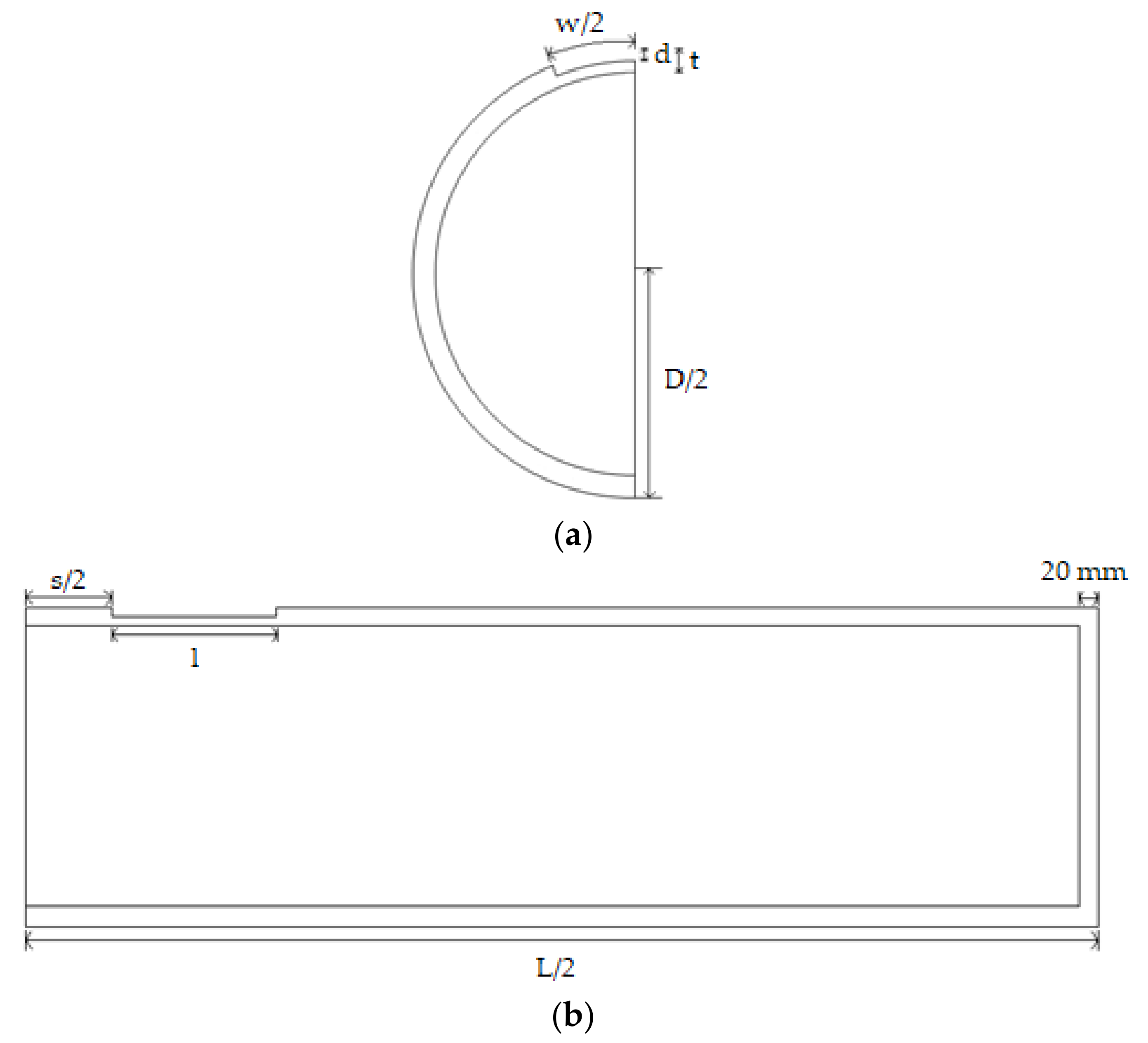
2.1.1. Generation of ANN Training Data
- Isothermal condition (constant temperature throughout the simulation).
- Isotropic and homogenous pipe model (uniform material properties in all directions).
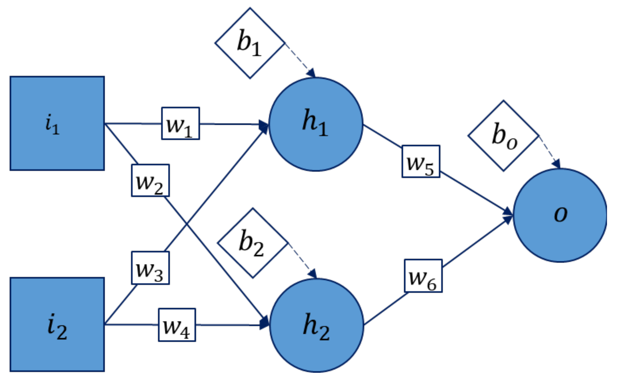
2.1.2. Training of the Artificial Neural Network
2.2. Development of the Empirical Equation
3. Results
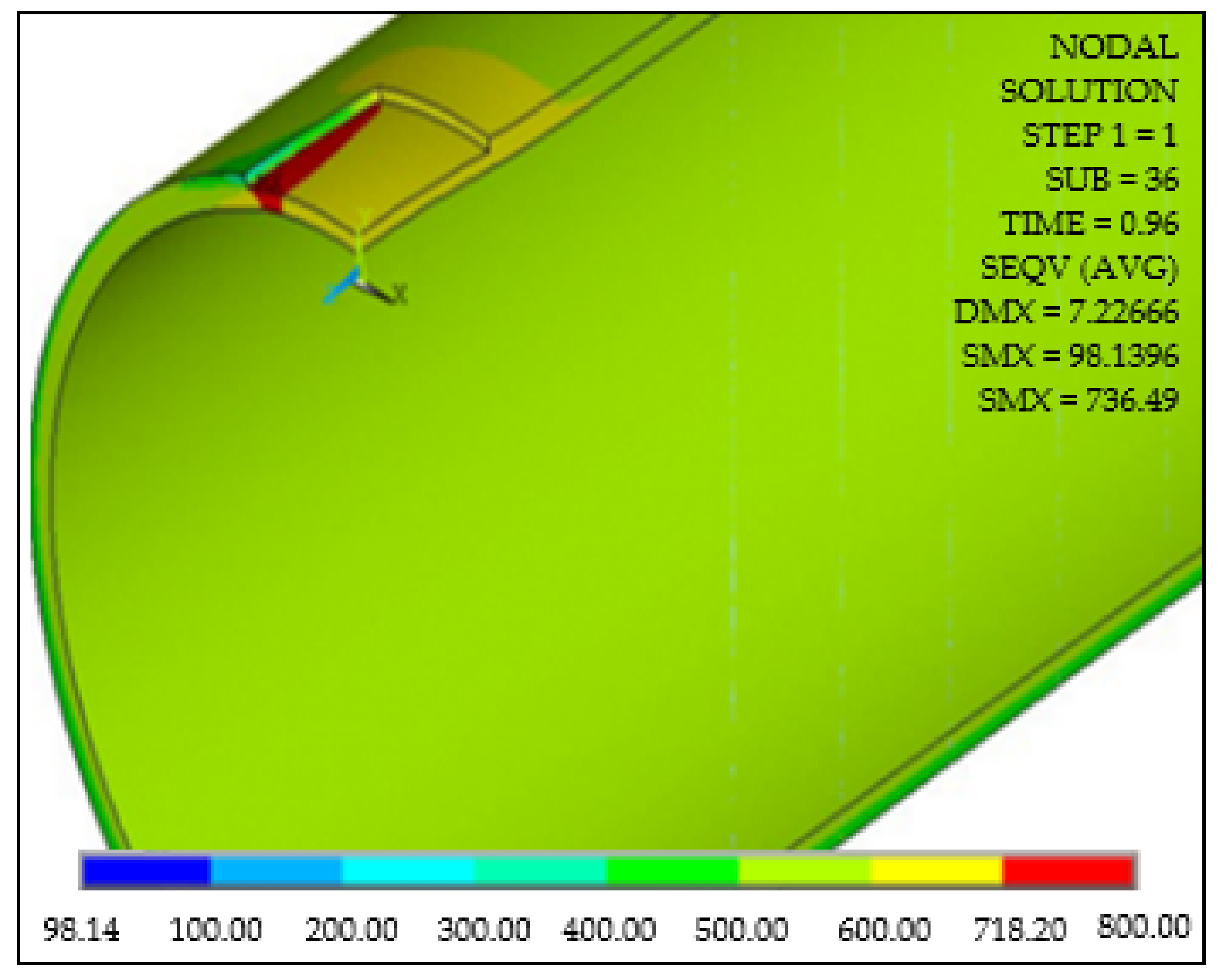
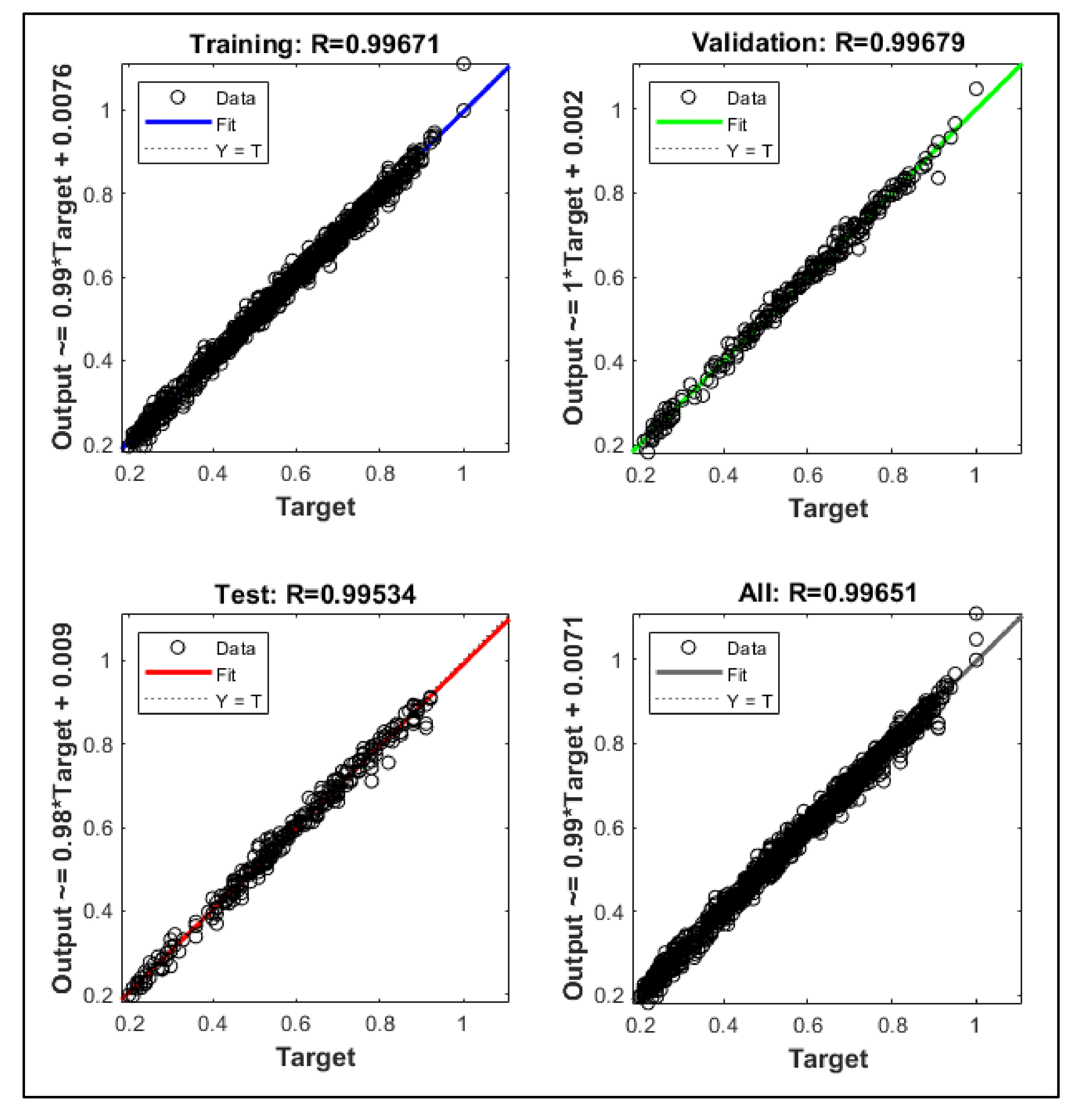
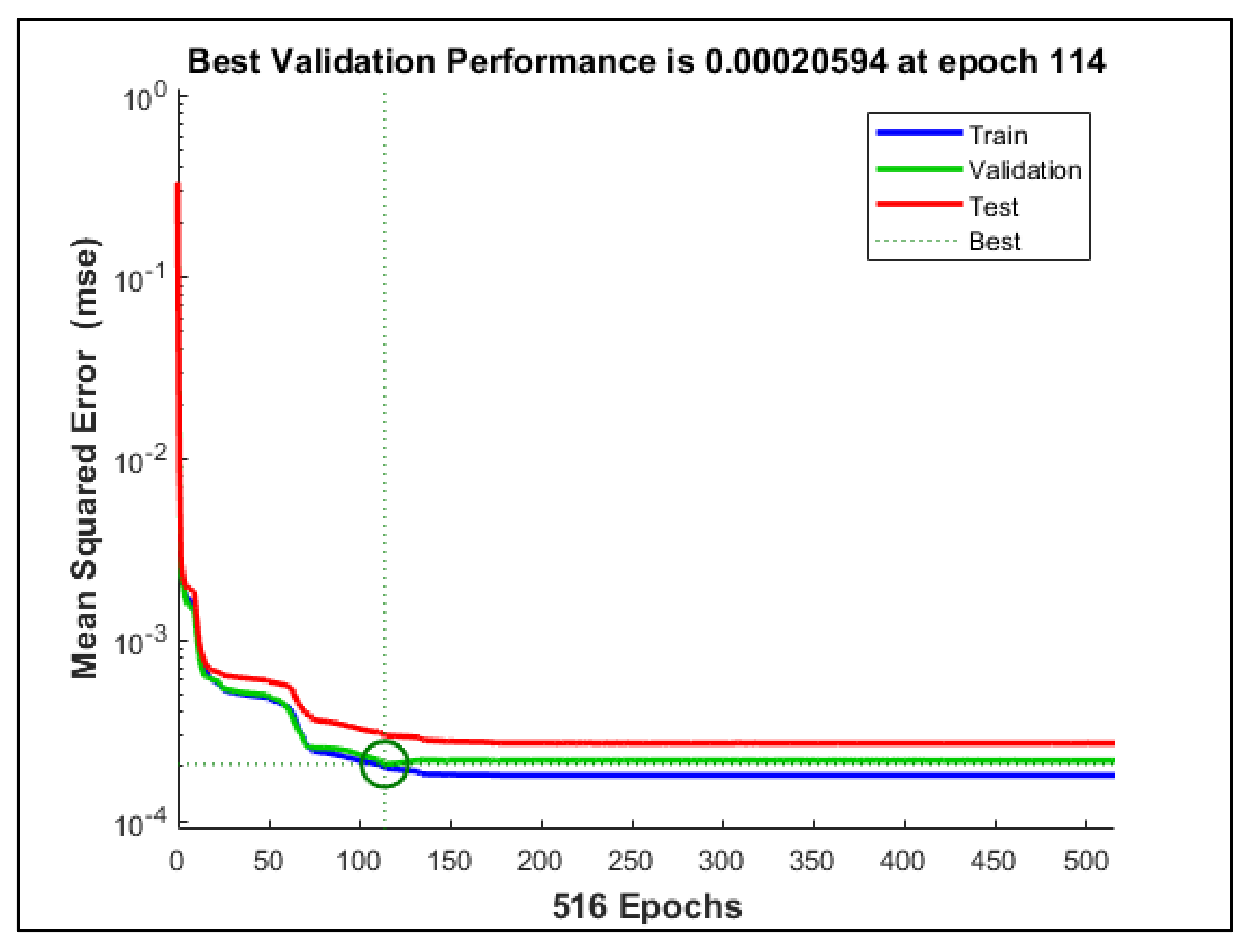
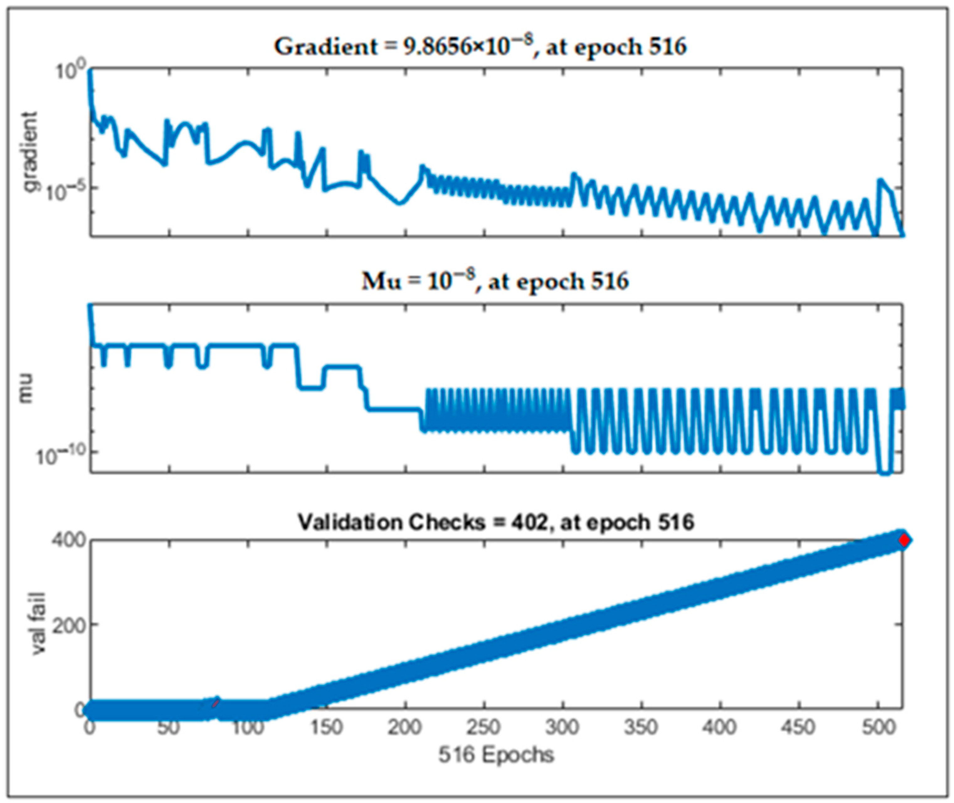
3.1. Development of Artificial Neural Network
3.2. Development of Empirical Equation
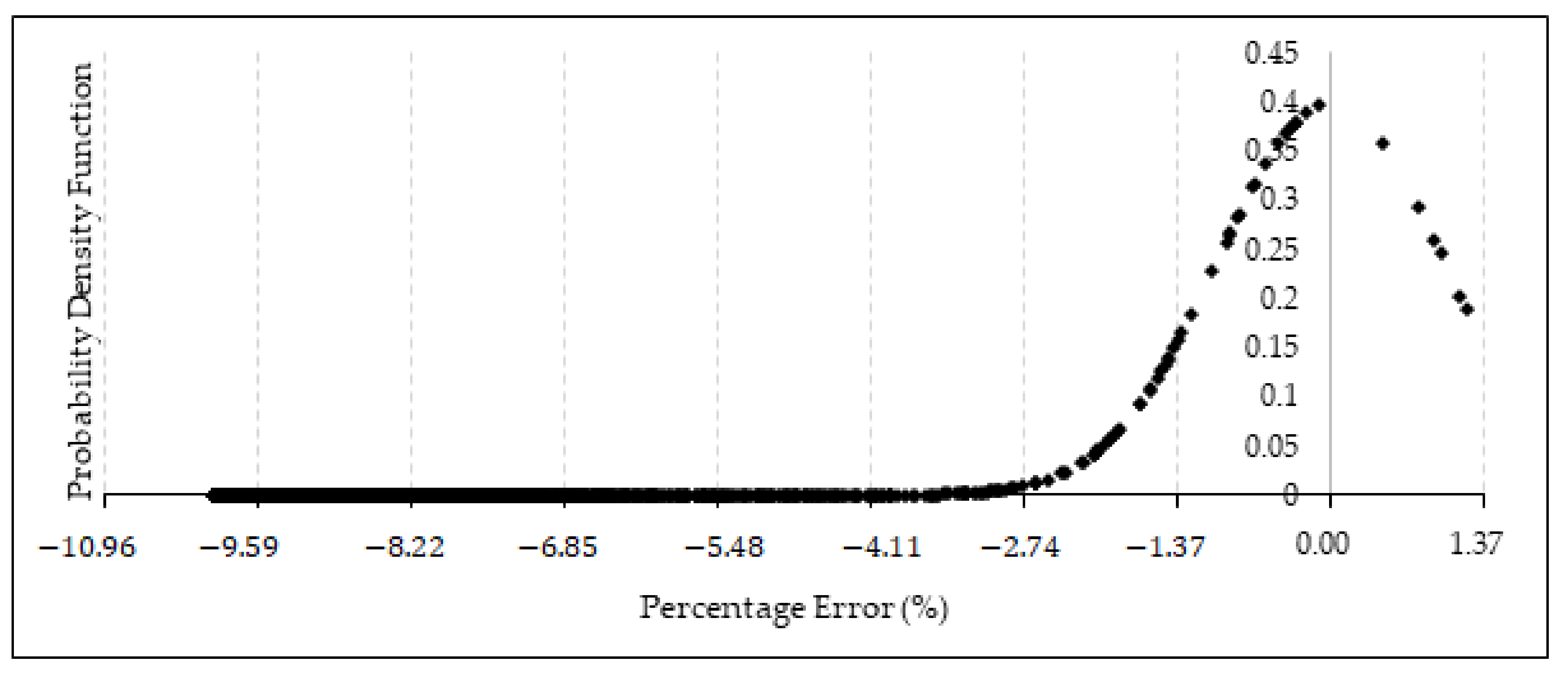
3.3. Evaluation of the Developed Empirical Failure Pressure Assessment Method
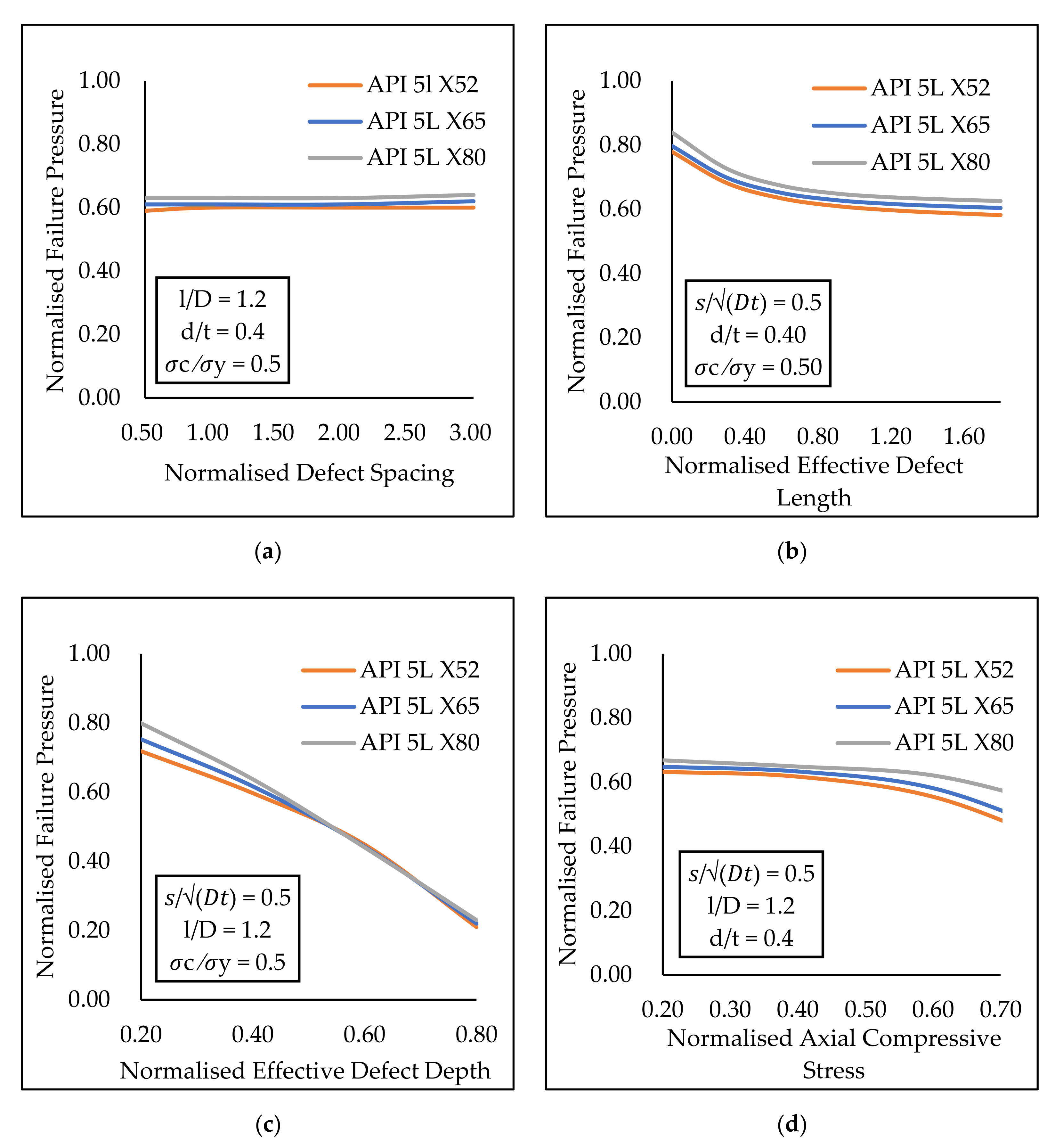
4. Extensive Parametric Studies Using the Developed Empirical Equation
5. Conclusions
Author Contributions
Funding
Institutional Review Board Statement
Informed Consent Statement
Data Availability Statement
Conflicts of Interest
Nomenclature
| Abbreviation | Unit | Description |
| ANN | - | Artificial neural network |
| DOF | - | Degree of freedom |
| FEA | - | Finite element analysis |
| FEM | - | Finite element method |
| mm | Pipe diameter | |
| Pa | Modulus of elasticity | |
| mm | Pipe length | |
| Pa | Pipe failure pressure | |
| - | Normalized pipe failure pressure obtained using the newly developed equation | |
| - | Normalized pipe failure pressure obtained using FEM | |
| Pa | Pipe intact pressure | |
| mm | Defect depth | |
| mm | Effective defect depth | |
| mm | Depth of defect number 1 | |
| mm | Depth of defect number 2 | |
| - | Input parameter value | |
| - | Maximum input parameter value | |
| - | Minimum input parameter value | |
| - | Normalized input parameter value | |
| - | Normalized maximum input parameter value | |
| - | Normalized minimum input parameter value | |
| mm | Defect length | |
| mm | Length of defect number 1 | |
| mm | Length of defect number 2 | |
| - | Neuron in hidden layer | |
| - | Output parameter value | |
| - | Maximum output parameter value | |
| - | Minimum output parameter value | |
| - | Normalized output parameter value | |
| - | Normalized maximum output parameter value | |
| - | Normalized minimum output parameter value | |
| mm | Pipe internal radius | |
| mm | Circumferential defect spacing | |
| mm | Longitudinal defect spacing | |
| mm | Pipe wall thickness | |
| - | Poisson’s ratio | |
| mm | Defect width | |
| Pa | Axial compressive stress | |
| Pa | Ultimate tensile strength | |
| Pa | True ultimate tensile strength | |
| Pa | Yield stress |
References
- Zeinoddini, M.; Arnavaz, S.; Zandi, A.P.; Vaghasloo, Y.A. Repair welding influence on offshore pipelines residual stress fields: An experimental study. J. Constr. Steel Res. 2013, 86, 31–41. [Google Scholar] [CrossRef]
- Shuai, Y.; Zhou, D.C.; Wang, X.H.; Yin, H.G.; Zhu, S.; Li, J.; Cheng, Y.F. Local buckling failure analysis of high strength pipelines containing a plain dent under bending moment. J. Nat. Gas. Sci. Eng. 2020, 77, 103266. [Google Scholar] [CrossRef]
- Zhang, Y.; Shuai, J.; Ren, W.; Lv, Z. Investigation of the tensile strain response of the girth weld of high-strength steel pipeline. J. Constr. Steel Res. 2022, 188, 107047. [Google Scholar] [CrossRef]
- Arumugam, T.; Karuppanan, S.; Ovinis, M. Finite element analyses of corroded pipeline with single defect subjected to internal pressure and axial compressive stress. Mar. Struct. 2019, 72, 102746. [Google Scholar] [CrossRef]
- Lo, M.; Karuppanan, S.; Ovinis, M. Failure Pressure Prediction of a Corroded Pipeline with Longitudinally Interacting Corrosion Defects Subjected to Combined Loadings Using FEM and ANN. J. Mater. Sci. Eng. 2021, 9, 281. [Google Scholar] [CrossRef]
- Kumar, S.D.V.; Karuppanan, S.; Ovinis, M. Failure Pressure Prediction of High Toughness Pipeline with a Single Corrosion Defect Subjected to Combined Loadings Using Artificial Neural Network (ANN). Metals 2021, 11, 373. [Google Scholar] [CrossRef]
- Belachew, C.T.; Ismail, M.C.; Karuppanan, S. Burst strength analysis of corroded pipelines by finite element method. J. Appl. Sci. 2011, 11, 1845–1850. [Google Scholar] [CrossRef]
- Kumar, S.D.V.; Lo, M.; Arumugam, T.; Karuppanan, S. A review of finite element analysis and artificial neural networks as failure pressure prediction tools for corroded pipelines. Materials 2021, 14, 6135. [Google Scholar] [CrossRef]
- Cosham, A.; Hopkins, P.; Macdonald, K.A. Best practice for the assessment of defects in pipelines—Corrosion. Eng. Fail. Anal. 2007, 14, 1245–1265. [Google Scholar] [CrossRef]
- DNV. Recommended Practice DNV-RP-F101. Available online: https://www.dnv.com/oilgas/download/dnv-rp-f101-corroded-pipelines.html#:~:text=This%20recommended%20practice%20(RP)%20provides,combined%20with%20longitudinal%20compressive%20stresses (accessed on 15 April 2022).
- Amaya-Gómez, R.; Sánchez-Silva, M.; Bastidas-Arteaga, E.; Schoefs, F.; Munoz, F. Reliability assessments of corroded pipelines based on internal pressure—A review. Eng. Fail. Anal. 2019, 98, 190–214. [Google Scholar] [CrossRef]
- Arumugam, T.; Kasyful, M.; Mohamad, A.; Saravanan, R. Burst capacity analysis of pipeline with multiple longitudinally aligned interacting corrosion defects subjected to internal pressure and axial compressive stress. SN Appl. Sci. 2020, 2, 1201. [Google Scholar] [CrossRef]
- Benjamin, A.C.; Freire, J.L.F.; Vieira, R.D. Analysis of pipeline containing interacting corrosion defects. A Ser. Appl. Exp. Tech. F. Pipeline Integr. 2007, 31, 74–82. [Google Scholar] [CrossRef]
- Li, F.; Wang, W.; Xu, J.; Yi, J.; Wang, Q. Comparative study on vulnerability assessment for urban buried gas pipeline network based on SVM and ANN methods. Process. Saf. Environ. Prot. 2019, 122, 23–32. [Google Scholar] [CrossRef]
- Silva, R.C.C.; Guerreiro, J.N.C.; Loula, A.F.D. A study of pipe interacting corrosion defects using the FEM and neural networks. Adv. Eng. Softw. 2007, 38, 868–875. [Google Scholar] [CrossRef]
- Xu, W.Z.; Li, C.B.; Choung, J.; Lee, J.M. Corroded pipeline failure analysis using artificial neural network scheme. Adv. Eng. Softw. 2017, 112, 255–266. [Google Scholar] [CrossRef]
- Chen, Y.; Zhang, H.; Zhang, J.; Liu, X.; Li, X.; Zhou, J. Failure assessment of X80 pipeline with interacting corrosion defects. Eng. Fail. Anal. 2015, 47, 67–76. [Google Scholar] [CrossRef]
- Kumar, S.D.V.; Karuppanan, S.; Ovinis, M. An empirical equation for failure pressure prediction of high toughness pipeline with interacting corrosion defects subjected to combined loadings based on artificial neural network. Mathematics 2021, 9, 582. [Google Scholar] [CrossRef]
- Tohidi, S.; Sharifi, Y.; Shari, Y. Thin-Walled Structures Load-carrying capacity of locally corroded steel plate girder ends using artificial neural network. Thin-Walled Struct. 2016, 100, 48–61. [Google Scholar] [CrossRef]
- de Andrade, E.Q.; Benjamin, A.C.; Machado, P.R., Jr.; Pereira, L.C.; Jacob, B.P.; Carneiro, E.G.; Guerreiro, J.N.; Silva, R.C.; Noronha, D.B., Jr. Finite element modeling of the failure behavior of pipelines containing interacting corrosion defects. In Proceedings of the 25th International Conference on Offshore Mechanics and Arctic Engineering—OMAE, Hamburg, Germany, 4–9 June 2006; pp. 315–325. [Google Scholar] [CrossRef]
- Sun, J.; Cheng, Y.F. Assessment by finite element modeling of the interaction of multiple corrosion defects and the effect on failure pressure of corroded pipelines. Eng. Struct. 2018, 165, 278–286. [Google Scholar] [CrossRef]
- ANSYS. ANSYS Theory Reference; ANSYS Inc.: Canonsburg, PA, USA, 2019. [Google Scholar]
- Wang, Y.-L.; Li, C.-M.; Chang, R.-R.; Huang, H.-R. State evaluation of a corroded pipeline. J. Mar. Eng. Technol. 2016, 15, 88–96. [Google Scholar] [CrossRef]
- Wiesner, C.S.; Maddox, S.J.; Xu, W.; Webster, G.A.; Burdekin, F.M. Engineering critical analyses to BS 7910—The UK guide on methods for assessing the acceptability of flaws in metallic structures. Int. J. Press. Vessel. Pip. 2001, 77, 883–893. [Google Scholar] [CrossRef]
- Cronin, D.S.; Pick, R.J. Prediction of the failure pressure for complex corrosion defects. Int. J. Press. Vessel. Pip. 2002, 79, 279–287. [Google Scholar] [CrossRef]
- Terán, G.; Capula-Colindres, S.; Velázquez, J.C.; Fernández-Cueto, M.J.; Angeles-Herrera, D.; Herrera-Hernández, H. Failure pressure estimations for pipes with combined corrosion defects on the external surface: A comparative study. Int. J. Electrochem. Sci. 2017, 12, 10152–10176. [Google Scholar] [CrossRef]
- Bjørnøy, O.H.; Sigurdsson, G.; Cramer, E. Residual Strength of Corroded Pipelines, DNV Test Results. In Proceedings of the Tenth (2000) International Offshore and Polar Engineering Conference, Seattle, DC, USA, 5–10 June 2000; Volume II, pp. 1–7. [Google Scholar]
- Benjamin, A.C.; Freire, J.L.F.; Vieira, R.D.; Diniz, J.L.C.; de Andrade, E.Q. Burst Tests on Pipeline Containing Interacting Corrosion Defects. In Proceedings of the 24th International Conference on Offshore Mechanics and Arctic Engineering (OMAE 2005), Halkidiki, Greece, 12–17 June 2005; pp. 1–15. [Google Scholar]
- Gurney, K. An Introduction to Neural Networks an Introduction to Neural Networks; UCL Press: London, UK, 1997. [Google Scholar]
- Chin, K.T.; Arumugam, T.; Karuppanan, S.; Ovinis, M. Failure pressure prediction of pipeline with single corrosion defect using artificial neural network. Pipeline Sci. Technol. 2020, 4, 10–17. [Google Scholar] [CrossRef]


| Method | Fundamental Equation | Governing Assumption | Material Restriction | Defect Idealization |
|---|---|---|---|---|
| ASME B31G | NG-18 | Failure pressure caused by flow-stress-dependent mechanism | Low toughness | Parabolic or rectangular |
| Modified B31G | NG-18 | Low toughness | Mixed shape | |
| SHELL 92 | NG-18 | - | Rectangular | |
| RSTRENG | NG-18 | Effective area | ||
| DNV RP-F101 | NG-18 | Pipe failure controlled by plastic flow (ultimate tensile strength is the flow stress) | Moderate toughness | Rectangular |
| Method | Advantage | Limitation |
|---|---|---|
| DNV-RP-F101 (most comprehensive) | Most comprehensive code for low- to medium-toughness pipes | Conservative Does not cater for interacting defects subjected to combined loading |
| Finite Element Method | Highly accurate Caters for all material grades and defect orientation | Complex Requires usage of software Time-consuming |
| Artificial Neural Network | Able to process complex nonlinear data Robust | Requires a large dataset for training and development |
| Properties | Pipe Body | Pipe End Cap | ||
|---|---|---|---|---|
| API 5L X52 | API 5L X65 | API 5L X80 | ||
| Modulus of elasticity, | 210.0 GPa | 200.0 TPa | ||
| Poisson’s ratio, | 0.3 | 0.3 | ||
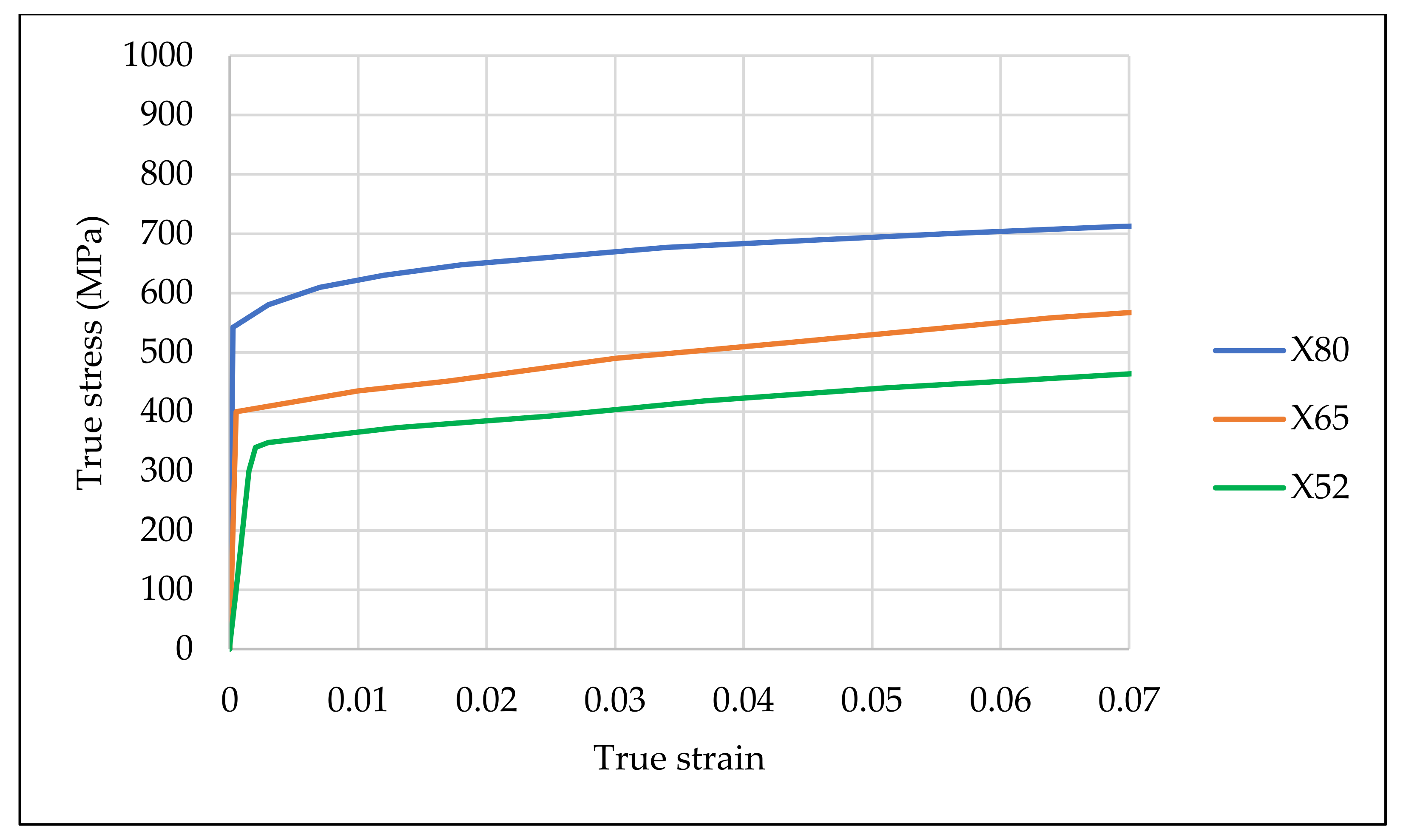
| Yield strength, | 359.0 MPa | 464.0 MPa | 534.1 MPa | - |
| True ultimate tensile strength, | 612.0 MPa | 629.0 MPa | 718.2 MPa | - |
| Input Parameters | Values |
| Outer diameter of pipe, (mm) | 300 |
| Length of pipe, (mm) | 2000 |
| Wall thickness, (mm) | 10 |
| Normalized defect width, | 10 |
| Normalized effective defect depth, | 0.00–0.80 |
| Normalized effective defect length, | 0.00–2.95 |
| Normalized longitudinal defect spacing, | 0.0– 3.00 |
| Normalized longitudinal compressive stress, | 0.00–0.80 |
| Number of Element Layers | |
|---|---|
| 1 | 0.92 |
| 2 | 0.93 |
| 3 | 0.95 |
| 4 | 0.95 |
| 5 | 0.95 |
| Grade | Specimen | d (mm) | l (mm) | w (mm) | σl (MPa) | ||
|---|---|---|---|---|---|---|---|
| X52 [27] | Test 1 | 5.15 | 243 | 154.5 | 0.0 | - | - |
| Test 5 | 3.09 | 162 | 30.9 | 48.0 | - | - | |
| Test 6 | 3.09 | 162 | 30.9 | 84.0 | - | - | |
| X80 [28] | IDTS 2 | 5.39 | 39.6 | 31.9 | - | 0.0 | 0.0 |
| IDTS 3 | 5.32 | 39.6 | 31.9 | - | 20.5 | 0.0 | |
| IDTS 4 | 5.62 | 39.6 | 32.0 | - | 0.0 | 9.9 |
| Specimen | Burst Pressure (MPa) | FEA Failure Pressure (MPa) | Percentage Difference (%) |
|---|---|---|---|
| Test 1 | 23.2 | 22.95 | −1.08 |
| Test 5 | 28.6 | 28.35 | −0.87 |
| Test 6 | 28.7 | 27.00 | −5.92 |
| IDTS 2 | 22.68 | 22.40 | −1.23 |
| IDTS 3 | 20.31 | 20.12 | −0.94 |
| IDTS 4 | 21.14 | 20.62 | −2.46 |
| Model | No. of Neurons in Hidden 1 | R2 Value |
|---|---|---|
| 1 | 1 | 0.9326 |
| 2 | 2 | 0.9358 |
| 3 | 3 | 0.9448 |
| 4 | 4 | 0.9542 |
| 5 | 5 | 0.9865 |
| 6 | 6 | 0.9854 |
| 7 | 7 | 0.9930 |
| 8 | 8 | 0.9929 |
| 9 | 9 | 0.9756 |
| 10 | 10 | 0.9686 |
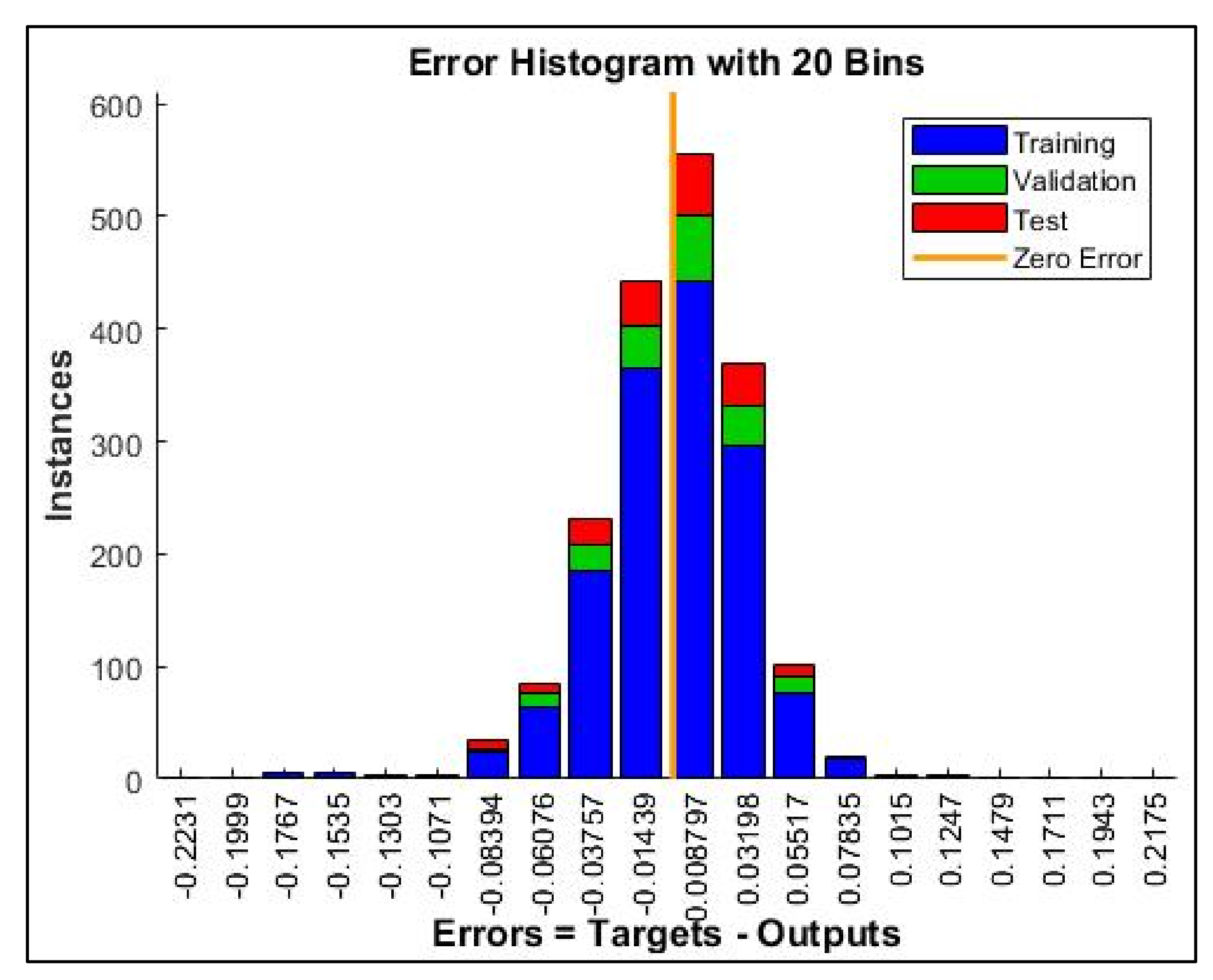
| Phase | R | MSE | RMSE | MAE | MAPE (%) |
|---|---|---|---|---|---|
| Training | 0.9967 | 0.0002 | 0.0141 | 0.0499 | −7.81 |
| Validation | 0.9967 | 0.0002 | 0.0141 | 0.0537 | −6.43 |
| Test | 0.9953 | 0.0003 | 0.0173 | 0.0325 | −5.35 |
| Percentage Difference | |||||||
|---|---|---|---|---|---|---|---|
| 612.0 | 0.00 | 0.45 | 0.20 | 0.25 | 0.80 | 0.73 | −9.21 |
| 612.0 | 0.50 | 0.35 | 0.45 | 0.55 | 0.60 | 0.57 | −4.95 |
| 612.0 | 1.00 | 0.85 | 0.35 | 0.60 | 0.59 | 0.55 | −7.49 |
| 612.0 | 2.00 | 0.40 | 0.35 | 0.25 | 0.75 | 0.69 | −7.43 |
| 612.0 | 2.50 | 1.20 | 0.20 | 0.20 | 0.76 | 0.72 | −5.28 |
| 612.0 | 3.00 | 2.00 | 0.50 | 0.60 | 0.48 | 0.43 | −9.94 |
| 612.0 | 3.50 | 0.35 | 0.45 | 0.55 | 0.64 | 0.59 | −7.51 |
| 612.0 | 3.00 | 0.45 | 0.20 | 0.25 | 0.83 | 0.77 | −7.59 |
| 612.0 | 0.00 | 0.35 | 0.45 | 0.55 | 0.59 | 0.54 | −8.06 |
| 612.0 | 0.50 | 1.60 | 0.50 | 0.10 | 0.52 | 0.47 | −8.97 |
| 612.0 | 1.05 | 2.00 | 0.75 | 0.30 | 0.28 | 0.27 | −4.56 |
| 612.0 | 2.25 | 2.40 | 0.20 | 0.20 | 0.74 | 0.69 | −6.85 |
| 612.0 | 2.50 | 0.45 | 0.20 | 0.25 | 0.82 | 0.76 | -7.40 |
| 612.0 | 3.75 | 2.00 | 0.50 | 0.60 | 0.47 | 0.43 | −8.88 |
| 612.0 | 3.50 | 0.40 | 0.35 | 0.25 | 0.78 | 0.70 | −9.77 |
| 612.0 | 3.00 | 0.35 | 0.45 | 0.55 | 0.65 | 0.59 | −8.80 |
| 612.0 | 0.00 | 0.45 | 0.20 | 0.25 | 0.75 | 0.73 | −3.16 |
| 612.0 | 0.50 | 0.35 | 0.45 | 0.55 | 0.60 | 0.54 | −9.60 |
| 612.0 | 1.00 | 0.85 | 0.35 | 0.60 | 0.58 | 0.54 | −6.91 |
| 629.0 | 2.00 | 1.20 | 0.20 | 0.20 | 0.78 | 0.73 | −6.23 |
| 629.0 | 2.50 | 2.00 | 0.50 | 0.10 | 0.50 | 0.45 | −9.90 |
| 629.0 | 3.00 | 2.00 | 0.50 | 0.60 | 0.35 | 0.34 | −3.32 |
| 629.0 | 3.50 | 0.40 | 0.35 | 0.25 | 0.53 | 0.48 | −8.78 |
| 629.0 | 0.00 | 0.45 | 0.20 | 0.25 | 0.84 | 0.77 | −8.88 |
| 629.0 | 0.50 | 2.40 | 0.75 | 0.30 | 0.27 | 0.26 | −5.20 |
| 629.0 | 1.00 | 0.45 | 0.20 | 0.20 | 0.80 | 0.77 | −3.60 |
| 629.0 | 2.00 | 0.35 | 0.45 | 0.25 | 0.65 | 0.62 | −4.53 |
| 629.0 | 2.50 | 0.85 | 0.35 | 0.55 | 0.58 | 0.55 | −5.30 |
| 629.0 | 3.00 | 2.00 | 0.50 | 0.60 | 0.35 | 0.34 | −3.32 |
| 629.0 | 3.25 | 0.40 | 0.35 | 0.25 | 0.55 | 0.52 | −5.22 |
| 629.0 | 0.00 | 0.40 | 0.35 | 0.25 | 0.70 | 0.69 | −1.69 |
| 629.0 | 0.50 | 1.20 | 0.20 | 0.60 | 0.69 | 0.64 | −7.47 |
| 629.0 | 1.00 | 2.00 | 0.50 | 0.60 | 0.48 | 0.45 | −6.30 |
| 629.0 | 2.00 | 2.40 | 0.75 | 0.20 | 0.23 | 0.22 | −2.61 |
| 629.0 | 2.50 | 0.40 | 0.45 | 0.10 | 0.60 | 0.56 | −6.49 |
| 629.0 | 3.50 | 0.35 | 0.45 | 0.55 | 0.28 | 0.28 | −1.22 |
| 629.0 | 3.00 | 0.45 | 0.20 | 0.25 | 0.66 | 0.61 | −7.57 |
| 629.0 | 0.00 | 0.40 | 0.35 | 0.25 | 0.76 | 0.69 | −9.45 |
| 718.2 | 0.50 | 0.45 | 0.35 | 0.25 | 0.77 | 0.71 | −8.08 |
| 718.2 | 1.00 | 0.35 | 0.20 | 0.55 | 0.79 | 0.76 | −3.72 |
| 718.2 | 2.00 | 0.85 | 0.50 | 0.10 | 0.57 | 0.52 | −8.60 |
| 718.2 | 2.50 | 0.85 | 0.50 | 0.10 | 0.45 | 0.42 | −7.11 |
| 718.2 | 3.00 | 0.40 | 0.35 | 0.25 | 0.45 | 0.45 | −0.35 |
| 718.2 | 0.00 | 2.00 | 0.75 | 0.30 | 0.28 | 0.26 | −5.92 |
| 718.2 | 0.50 | 2.40 | 0.45 | 0.20 | 0.58 | 0.54 | −6.39 |
| 718.2 | 1.00 | 0.40 | 0.35 | 0.25 | 0.76 | 0.71 | −6.64 |
| 718.2 | 2.00 | 0.45 | 0.20 | 0.55 | 0.80 | 0.75 | −6.83 |
| 718.2 | 2.50 | 0.35 | 0.50 | 0.20 | 0.46 | 0.42 | −8.37 |
| 718.2 | 3.00 | 0.40 | 0.35 | 0.25 | 0.45 | 0.45 | −0.35 |
| 718.2 | 2.35 | 0.40 | 0.35 | 0.25 | 0.64 | 0.58 | −9.77 |
Publisher’s Note: MDPI stays neutral with regard to jurisdictional claims in published maps and institutional affiliations. |
© 2022 by the authors. Licensee MDPI, Basel, Switzerland. This article is an open access article distributed under the terms and conditions of the Creative Commons Attribution (CC BY) license (https://creativecommons.org/licenses/by/4.0/).
Share and Cite
Vijaya Kumar, S.D.; Lo, M.; Karuppanan, S.; Ovinis, M. Empirical Failure Pressure Prediction Equations for Pipelines with Longitudinal Interacting Corrosion Defects Based on Artificial Neural Network. J. Mar. Sci. Eng. 2022, 10, 764. https://doi.org/10.3390/jmse10060764
Vijaya Kumar SD, Lo M, Karuppanan S, Ovinis M. Empirical Failure Pressure Prediction Equations for Pipelines with Longitudinal Interacting Corrosion Defects Based on Artificial Neural Network. Journal of Marine Science and Engineering. 2022; 10(6):764. https://doi.org/10.3390/jmse10060764
Chicago/Turabian StyleVijaya Kumar, Suria Devi, Michael Lo, Saravanan Karuppanan, and Mark Ovinis. 2022. "Empirical Failure Pressure Prediction Equations for Pipelines with Longitudinal Interacting Corrosion Defects Based on Artificial Neural Network" Journal of Marine Science and Engineering 10, no. 6: 764. https://doi.org/10.3390/jmse10060764