ANN- and FEA-Based Assessment Equation for a Corroded Pipeline with a Single Corrosion Defect

Abstract

Most of the standards available for the assessment of the failure pressure of corroded pipelines are limited in their ability to assess complex loadings, and their estimations are conservative. To overcome this research gap, this study employed an artificial neural network (ANN) model trained with data obtained using the finite element method (FEM) to develop an assessment equation to predict the failure pressure of a corroded pipeline with a single corrosion defect. A finite element analysis (FEA) of medium-toughness pipelines (API 5L X65) subjected to combined loads of internal pressure and longitudinal compressive stress was carried out. The results from the FEA with various corrosion geometric parameters and loads were used as the training dataset for the ANN. After the ANN was trained, its performance was evaluated, and its weights and biases were obtained for the development of a corrosion assessment equation. The prediction from the newly developed equation has a good correlation value, R² of 0.9998, with percentage errors ranging from −1.16% to 1.78%, when compared with the FEA results. When compared with the failure pressure estimates based on the Det Norske Veritas (DNV-RP-F101) guidelines, the standard was more conservative in its prediction than the assessment equation developed in this study.

1. Introduction

Pipelines are essential components in the continuous supply of natural gas from gas wells to refinery plants and storage facilities. The residual strength assessment of corroded pipelines is an indispensable part of maintaining continuous operation while protecting the environment. Corrosion reduces the wall thickness of pipelines, thereby weakening their strength due to the concentration of stress in the corrosion region [1]. Real corrosion in pipelines often takes the form of irregular geometric shapes, as shown in Figure 1. The complex shapes of corrosion defects discontinue the cylindrical symmetry of pipes, thereby affecting their structural strength [2]. As real corrosion defects are complex and difficult to model and assess due to their asymmetries, they are often simplified into regular shapes, such as parabolic and rectangular shapes.

Numerous assessment standards for evaluating the residual strength of corroded pipelines, such as American Society of Mechanical Engineers (ASME) B31G and Modified B31G, RSTRENG Effective Area, PCORRC, and DNV RP-F101, are widely practiced in the oil and gas industry, to inspect and maintain the operation of pipelines. However, most of these assessment standards are limited to corroded pipelines with a single defect, subjected to internal pressure only. DNV-RP-F101 is the most comprehensive standard out of them, which allows for the assessment of corroded pipelines subjected to combined loadings of internal pressure and longitudinal compressive stress. In subsea or geologically active regions, external loadings, such as external pressure and longitudinal stresses, should be considered. Longitudinal stresses are generally caused by soil movement, the free span of pipelines over seabed depressions or elevations, and large temperature variation between the content of pipelines and their surroundings. Longitudinal compressive stress causes buckling and wrinkling failure, which in turn reduces the residual strength of corroded pipelines when they are subjected to combined loadings [3,4,5].

Both experimental and numerical studies have been carried out to understand the failure of pipelines subjected to the combined loadings of internal pressure and longitudinal stress. Bjørnøy et. al (2000) carried out full-scale burst tests on twelve American Petroleum Institute (API) 5L-X52-grade steel pipelines with artificially created corrosion defects as part of the development of DNV RP-F101 assessment standards for corroded pipelines [6]. Their work revealed the significant effects of the bending moment and axial compressive stress on the residual strength of pressurized corroded pipelines, especially those with deep corrosion defects. Bjørnøy et al.’s work was supported by findings from Chauhan et al. (2009)’s work on high strength pipelines and Halima and Sreekanta (2017)’s studies on X46 corroded steel pipelines [7,8].

Of all the established corrosion assessment standards, DNV RP-F101 is the most comprehensive, as it is the only one that can be used to assess single-defect corroded pipelines subjected to internal pressure and longitudinal compressive stress. However, DNV RP-F101 is conservative in its assessment due to the assumptions and simplifications it involves. Meanwhile, numerical methods have proven to be better than the established standards for assessing the residual strength of corroded pipelines [9]. Numerical methods, such as the finite element method (FEM), were widely employed to verify and validate the failure behaviour and failure pressure of corroded pipelines [10,11,12,13]. They are especially useful for parametric studies with varying corrosion geometries, which would otherwise be too costly to be carried out experimentally. Despite the advantages of FEM, the numerical method is computationally expensive. Comprehensive parametric studies of varying corrosion defect geometry through FEM can be time intensive.

A few studies have used the results from the FEA to develop analytical solutions that can be deployed as quickly as standards and codes while retaining the accuracy of FEM. Buckingham’s π theorem has been used to develop closed-form expression using the results of a parametric study on corroded pipelines with single defects subjected to internal pressure [14,15]. Arumugam et al. (2020) used the theorem to develop new corrosion assessment equations for the failure of single-defect pipes when they are subjected to combined loadings of axial compressive stress and internal pressure [16]. The equations predicted the failure pressure with good margins of error (less than 10%).

With the adoption of machine learning, such as artificial neural networks (ANNs), as prediction tools, a handful of studies have used ANN to predict the failure pressure of corroded pipelines. The ANN models developed from these studies are modeled after a data-driven machine learning framework. The dataset used to train these ANN models was derived from results from experimental work, such as the full-scale burst testing of corroded pipelines, and results from numerical analyses using FEM.

Table 1. Literature on ANN application using FEA dataset to predict failure pressure of corroded pipeline.

Source	Corrosion Type	Loads	Material	ANN Architecture
Silva et al. [17]	Interacting defects (longitudinally and circumferentially aligned)	Internal pressure	X52	Feedforward neural network with backpropagation learning algorithm. (2-3-1).
Xu et al. [18]	Single and interacting defects (longitudinally and circumferentially aligned)	Internal pressure	X80	Feedforward neural network with backpropagation learning algorithm. (4-5-1).
Lu and Liang [19]	Single defects	Internal pressure and axial compressive load	X62, X70, X80	Not specified (4-6-6-1)
Khalajestani et al. [20]	Single defects on elbow	Internal pressure	Low- and mid-strength pipe	Feedforward neural network with Levenberg-Marquardt backpropagation learning algorithm (7-7-14-1)
Khalajestani and Bahaari [21]	Interacting defects on elbow	Internal pressure	Low- and mid-strength pipe	Feedforward neural network with Levenberg-Marquardt backpropagation learning algorithm (8-9-15-1)

shows the literature that used ANN in combination with FEA results to predict the failure pressure of corroded pipelines.

However, the ANN from the studies does not provide the ease of use as a closed-form expression. Tohidi and Sharifi (2016) developed closed-form expression from their ANN to predict the load-carrying capacity of locally corroded steel plate girder ends [22]. Kumar et al. (2021) developed assessment equations for high-strength pipelines with single defects subjected to axial load and internal pressure using ANN and FEA results, while Lo et al. (2021) developed assessment equations for mid-strength pipelines with longitudinally interacting defects subjected to longitudinal compressive stress and internal pressure using ANN and FEA results [23,24]. Their assessment equations showed accurate predictions with errors of less than 10%.

The objective of this paper is to employ ANNs together with the FEM to develop an analytical solution that predicts the failure pressure of corroded mid-strength pipelines with varying single-corrosion-defect geometries subjected to combined loads of internal pressure and longitudinal compressive stress. This paper addresses the conservatism of the standards and codes that are conventionally used to assess corroded pipelines while maintaining the accuracy of the FEA without intensive computation, using an analytical solution developed from ANNs.

2. Materials and Methods

This study uses FEM as a basis for developing a new corrosion assessment equation for steel pipelines with single corrosion defects subjected to both internal pressure and longitudinal compressive stress. The FEM was validated before generating a database of FEA results from selected corrosion geometric parameters and load application. Development of ANNs depends on the dataset used for training; therefore, the ANN model must be tailored to suit the shape (number of features and labels) and size (number of observations) of input dataset. The performance of the trained ANN model was evaluated before its weights and biases were used as a basis for the corrosion assessment equation.

2.1. Finite Element Method

The FEM from T. Arumugam (2020) is reproduced in this paper, with API 5L X65 grade steel pipeline as the material of the study using ANSYS (16.1) Mechanical ANSYS Parametric Design Language (APDL) [16]. The pipe model in this parametric study has an external diameter of $D_e=300 \mathrm{mm}$, a wall thickness of $t=10 \mathrm{mm}$, and a length of $L=2000 \mathrm{mm}$. The complex profile of a real corrosion defect is often idealized into simple shapes, such as rectangular, elliptical, and parabolic in FEM for ease of assessment. The corrosion defect of the model used is rectangular, with varying defect depths, defect lengths, and defect widths, as shown in

Table 2. Parameters of corrosion defect geometries and external load.

Defect Depth		Defect Length		Defect Width		Longitudinal Compressive Stress
d/t	d (mm)	l/D	l (mm)	w/t	w (mm)	${\mathit{\sigma }}_{\mathit{c}}/{\mathit{\sigma }}_{\mathit{y}}$	${\mathit{\sigma }}_{\mathit{c}} \left(\mathbf{MPa}\right)$
0.2	2	0.2	60	2	20	0.2	92.8
0.4	4	0.4	120	6	60	0.4	185.6
0.5	5	0.8	240	10	100	0.5	232.0
0.6	6	1.2	360	14	140	0.6	278.4
0.8	8	1.8	540	18	180	0.8	371.2
						1.0	464.0

. Conventional assessment standards often recommend modeling rectangular defects to assess corroded pipelines for additional levels of conservatism [25]. it is recommended to model a pipe end cap for application of longitudinal compression load, to reduce error between simulation and test results [11]. The varying longitudinal compressive stress is distributed equally onto the end cap, as shown in Table 2.

The symmetry of the rectangular corrosion defect and cylindrical pipe model can be exploited to reduce the computational time in the FEM. It is only necessary to model a quarter model, with appropriate application of boundary conditions, such as loads and constraints, to produce the same outcome as a full model. The dimension of the quarter-pipe model is illustrated in Figure 2, with annotation of its dimension and the areas where the boundary conditions were applied. The internal load (internal pressure) was applied on the internal surface areas of the pipe and the external load (longitudinal compressive stress) was applied on the surface of the end cap, as shown in Figure 3. Timesteps were used to apply the loads incrementally, through ramped loading in ANSYS. For cases of internal load only, the internal pressure was applied in the first and only timestep. For cases of internal load and external load, longitudinal compressive stress was applied incrementally in the first timestep. The internal pressure was applied incrementally in the second timestep, while external load of previous timestep was maintained.

The elements of the pipe body were meshed with hexahedral SOLID185 element in ANSYS. There were eight nodes in the element with three degrees of freedom in x, y, and z directions. The pipe end cap was meshed with higher-order element, SOLID186, which has 20 nodes. The element can tolerate the boundary curvature of pipe end cap without losing accuracy. Solid elements are preferred over shell elements when modeling pipe with corrosion defect. The British Standards Institution recommended at least two-to-four layers of elements to be meshed over the thickness of the pipe for accurate FEM; therefore, six layers of elements were modeled in this study [26]. Multi-point constraint was used to prevent unwanted rigid motion of pipe model when external load of longitudinal compressive stress was applied [16,27,28]. Three nodes near the end cap region and far away from corrosion defect were constrained in all directions, as denoted with triangle symbols in Figure 4. Preliminary analysis showed negligible difference between number of constrained nodes and their position (only in the region at the end of the pipe model, circled) with solution convergence.

A mesh convergence study was performed to identify the optimum mesh layers and computational time with reasonable solution accuracy (less than 10% percentage difference from burst test’s failure pressure). The results were tabulated in

Table 3. Results of mesh convergence study.

No. of Element Layers	$\mathbf{Normalized} \mathbf{Failure} \mathbf{Pressure}, {\mathit{P}}_{\mathit{f}}/{\mathit{P}}_{\mathit{i}}$
1	0.53
2	0.57
3	0.59
4	0.59
5	0.59
6	0.59

. According to the study, the optimum number of layers across the thickness of pipe was three elements. The region of interest was designated with high density of elements. A smaller element size was selected for the region of interest at the corrosion defect. The element size of the pipe model increased gradually when transitioning away from the corrosion defect, as depicted in Figure 3, to halve simulation time without sacrificing solution accuracy.

The Newton–Raphson (NR) method was applied for the static non-linear structural analysis, due to the non-linearity of the API 5L X65 grade steel pipe. Datapoints from the non-linear true stress–strain curve of the pipe (in Figure 5) were used for the SOLID185 elements in ANSYS and shown in

Table 4. Datapoints of X65 true stress–strain inputted into ANSYS.

No.	True Stress (MPa)	True Strain	No.	True Stress (MPa)	True Strain
1	0	0	17	817.28	0.5491
2	465.43	0.0022	18	826.72	0.5910
3	479.87	0.0272	19	836.43	0.6328
4	507.37	0.0461	20	845.72	0.6747
5	548.38	0.0671	21	853.38	0.7166
6	615.55	0.0938	22	861.04	0.7585
7	648.26	0.1301	23	868.01	0.8004
8	678.35	0.1720	24	875.26	0.8422
9	702.41	0.2139	25	882.24	0.8841
10	722.93	0.2558	26	888.80	0.9260
11	741.39	0.2977	27	895.23	0.9679
12	756.43	0.3396	28	900.97	1.0098
13	770.51	0.3815	29	907.26	1.0516
14	783.78	0.4234	30	912.87	1.0935
15	794.99	0.4653	31	919.02	1.1354
16	806.61	0.5072	32	923.28	1.1677

.

The pipe end cap was considered as a rigid body, as its purpose was to transfer longitudinal stress onto the pipe body. To prevent deformation of the end cap when a large load was applied on it, a high stiffness was used.

Table 5. Mechanical properties of API 5L X65 steel pipe.

	Pipe Body (API 5L X65)	Pipe End Cap (Rigid Body)
Modulus of Elasticity, E	210 GPa	210 TPa
Poisson’s ratio, $v$	0.3	0.3
$\mathrm{Yield} \mathrm{Strength}, {\sigma }_y$	464 MPa	-
$\mathrm{Ultimate} \mathrm{tensile} \mathrm{strength}, {\sigma }_u$	563 MPa	-
$\mathrm{True} \mathrm{ultimate} \mathrm{tensile} \mathrm{strength}, {\sigma }_u*$	629 MPa	-

summarizes the mechanical properties of the pipe body and end cap.

The failure criterion adopted for this FEM was based on the work by Choi et al. on the limit load development of corroded X65 gas pipelines [30]. The failure mechanism is dictated by plastic collapse of steel pipe, which occurs when the von Mises stress reaches the reference stress (ultimate tensile strength) across the entire wall thickness, as shown by red contour in Figure 6. In Choi et al.’s work, their reference stress was 80% of the material’s ultimate strength for rectangular-shaped defects and 90% of ultimate strength for elliptical-shaped defects. This paper employed the true ultimate tensile strength (UTS) of X65 grade steel pipe as the reference stress because true UTS provides more accurate results [16,18]. The corresponding applied internal pressure is the failure pressure when the failure criterion is fulfilled.

2.2. Finite Element Method Validation

The FEM was validated with results from full-scale burst tests. Results from full-scale burst test by Kim et al. [31] and Ma et al. [32] were used for validation of FEM on single corrosion defect subjected to internal pressure only. Kim et al. performed their burst test on corroded X65 pipe with a 762 mm outer diameter, 17.5 mm wall thickness, and 2.3 m length pipe specimen enclosed with end caps at pipe ends. Ma et al. compiled results of full-scale burst tests for different grades of corroded pipe, from X42 to X100. The dimensions of X65 pipe in Ma et al.’s dataset is the same as those of the corroded pipes in Kim et al.’s study. Specimens LD and LF were chosen from Kim et al.’s work and No. 61, No. 62, and No. 63 were chosen from Ma et al.’s work for FEM validation, due to their variety of corrosion defect length and corrosion defect depth, respectively. The geometric properties of single corrosion defects chosen for FEM validation are tabulated in

Table 6. Dimension of corrosion defects and applied longitudinal compressive stress of selected specimens for FEM validation.

Specimen	d (mm)	l (mm)	w (mm)	${\mathit{\sigma }}_{\mathit{c}} \left(\mathbf{MPa}\right)$
Validation for internal pressure only.
LD	8.75	50.00	50.00	-
LF	8.75	100.00	50.00	-
No. 61	4.40	200.00	600.00	-
No. 62	8.80	200.00	600.00	-
No. 63	13.10	200.00	600.00	-
Validation for internal pressure and longitudinal compressive stress.
Test 5	3.09	162.00	30.90	48.00
Test 6	3.09	162.00	30.90	84.00

.

The FEM on corroded pipe subjected to both internal pressure and longitudinal compressive stress was validated with results of full-scale burst tests performed by Bjørnøy et al. [6]. The burst tests were conducted on X52 steel pipes with a single corrosion defect on the pipe body with 324-millimeter outer diameter, 10.3-millimeter wall thickness, and 1.0-meter length. Only the material property of the FE models was replaced with API 5L X52 grade steel, while the meshing and boundary conditions remained the same. The parameters of the selected burst tests are shown in Table 6.

The burst tests were modeled with previously proposed FEM framework and material properties were incorporated in elements of the FE model. The results from the FEA are tabulated in

Table 7. Failure pressure from burst tests compared with failure pressure predicted in FEA.

Specimen	Failure Pressure from Burst Tests (MPa)	Failure Pressure Predicted in FEA (MPa)	Absolute Percentage Difference (%)
Validation for internal pressure only.
LD	19.80	20.1	1.50
LF	15.00	15.50	3.67
No. 61	24.11	23.70	1.70
No. 62	21.76	21.30	2.11
No. 63	17.15	17.10	0.29
Validation for internal pressure and longitudinal compressive stress.
Test 5	28.60	29.20	2.10
Test 6	28.70	29.60	3.14

. The difference between failure pressure on burst tests and failure pressure in FEA prediction was relatively small, with a maximum absolute percentage difference of 3.67%.

2.3. Machine Learning and Artificial Neural Network

Machine learning (ML) is a general method of extracting patterns and trends using modern computing [33]. The technique makes predictions or decisions based on given datasets through programmed algorithms. Different ML techniques are used to solve different types of problem, such as regression and classification problems [34]. Predicting failure pressure to assess fitness-of-service of a corroded pipeline is a regression problem. A regression problem is when the desired output is a continuous value, such as failure pressure. Artificial neural networks (ANNs) are a ML technique that is best suited to solving regression problems because of their ability to characterize complex nonlinear relationships in a given dataset [33]. There are different approaches to the application of ML to problems, namely supervised learning, unsupervised learning, and reinforcement learning. The difference between these approaches depends on the level of information given to the computer to learn. In supervised learning, the computer is given most of the available data, which include the input with labeled target output to be trained on. The computer and ML algorithm then map the relationship between input and target output and perform predictions based on the given dataset. Supervised learning is employed. Feed-forward neural network (FFNN) architecture comprising an input layer, hidden layer(s), and an output layer, was selected for this study. When multiple neurons are linked with each other in layers, an artificial neural network is formed. ANNs are based on the universal approximation theory, which states that a simple neural network can approximate continuous functions of given inputs. In this work, ANN algorithm was developed using the results of an FE analysis to derive a new empirical formula for better prediction of residual strength of corroded pipelines subjected to combined loadings.

Every neural network has unique architecture. The number of hidden layers and number of hidden neurons of the network depend on the application of the neural network and training data sample available. Therefore, a tailored ANN development framework was needed for this study. The input and output of the ANN were obtained from the solution of the FEA on corroded X65 pipeline. The data were then cleaned before being feeding into the neural network. A neural network was created with a training algorithm to train on the processed input and target output. The performance of ANN was measured based on the error between predicted output and target output and improved by adjusting its hyperparameters appropriately. The framework to develop ANN algorithm to predict failure pressure of corroded pipeline is illustrated as a flowchart in Figure 7.

An iteration of the training process of the neural network is illustrated in Figure 8, which is a part of the ANN development process flow shown in Figure 7. Typically, in FFNN, inputs are propagated forward through randomly initialized weights to predict the output. A cost function is employed to measure the performance of FFNN by quantifying the error between the predicted output and expected output. Training algorithms, such as backpropagation, are used to update the weights to minimize the cost function. The Levenberg–Marquardt (LM) backpropagation algorithm was used to train FFNN. LM algorithm performs more efficiently compared to other learning rules as it requires less time and epochs for convergence because it uses a second-order convergence rate [35].

After the ANN was trained, its performance was evaluated against part of dataset for validation and testing purposes. The results from FEA were divided into train, validation, and test sets, where the input and target output were randomly divided in the following proportions: 80% for training, 10% for validation, and 10% for testing. Validation and test sets were used to prevent overfitting, which is akin to over-training. As the network began to overfit the datapoints, the error on the validation and test sets increased. The performance of the ANN was evaluated through coefficient of determination (R²), mean squared error (MSE), and mean absolute error (MAE).

$${\mathrm{R}}^2={(\frac{{{\displaystyle \sum }}_{\mathrm{i}=1}^{\mathrm{N}}\left({\mathrm{y}}_{\mathrm{i}} - {\overline{\mathrm{y}}}_{\mathrm{i}}\right)\left({\hat{\mathrm{y}}}_{\mathrm{i}}-{\overline{\hat{\mathrm{y}}}}_{\mathrm{i}}\right)}{\sqrt{{{\displaystyle \sum }}_{\mathrm{i}=1}^{\mathrm{N}}{\left({\mathrm{y}}_{\mathrm{i}}-{\overline{\mathrm{y}}}_{\mathrm{i}}\right)}^2{{\displaystyle \sum }}_{\mathrm{i}=1}^{\mathrm{N}}{({\hat{\mathrm{y}}}_{\mathrm{i}}-{\overline{\hat{\mathrm{y}}}}_{\mathrm{i}})}^2}})}^2$$

(1)

$$\mathrm{MSE}=\frac{1}{\mathrm{N}}{\displaystyle \sum }_{\mathrm{i}=1}^{\mathrm{N}}{\left({\hat{\mathrm{y}}}_{\mathrm{i}}-{\mathrm{y}}_{\mathrm{i}}\right)}^2$$

(2)

$$\mathrm{MAE}=\frac{1}{\mathrm{N}}{\displaystyle \sum }_{\mathrm{i}=1}^{\mathrm{N}}\left|{\mathrm{y}}_{\mathrm{i}}-{\hat{\mathrm{y}}}_{\mathrm{i}}\right|$$

(3)

where ${\widehat{y}}_i$ and $y_i$ are the actual and predicted output values for the ith output, respectively. ${\overline{\widehat{y}}}_i$ and ${\overline{y}}_i$ are the average of actual and predicted output, and N is the number of samples. R², or squared correlation coefficient, is the evaluation of goodness-of-fit for the predicted value against actual value, where R² value of 1.00 corresponds to perfect fit. The MSE is the sum of squared difference between the predictions and actual values. The MAE is the average absolute error between predictions and actual values, which measures the accuracy of the predictions.

Generally, trial-and-error methods are employed to determine the number of hidden layers, and number of hidden neurons. A handful of research studies tried to formulate a one-size-fits all equation to determine the optimum number of hidden neurons. Equation (4) is one of the many equations to calculate number of hidden neurons [36]:

$$N_h=\frac{\left(4p^2+3\right)}{\left(p^2-8\right)}$$

(4)

where $N_h$ is the number of hidden neurons and $p$ is the number of input variables of the network. The calculated number of hidden neurons was used as reference point to prune the hyperparameters of the neural network.

3. Results

3.1. Preliminary Finite Element Analysis

A preliminary study was performed to better understand the failure pressure trends in different geometric parameters of a single corrosion defect. The geometry of the corrosion defect was varied one factor at a time. The tests were prefixed with SDOFAT (Single defect: One factor at a time).

Table 8. FEA on corroded pipeline with single corrosion defect subjected to internal pressure and longitudinal compressive stress, one factor at a time.

Test Models	Defect Parameters			External Load	Normalized Failure Pressure
	d/t	l/D	w/t	${\mathit{\sigma }}_{\mathit{c}}\mathbf{/}{\mathit{\sigma }}_{\mathit{y}}$	FEA	DNV
SDOFAT1	0.2	0.8	10	-	0.82	0.75
SDOFAT2	0.4	0.8	10	-	0.68	0.61
SDOFAT3	0.5	0.8	10	-	0.59	0.53
SDOFAT4	0.6	0.8	10	-	0.49	0.45
SDOFAT5	0.8	0.8	10	-	0.28	0.25
SDOFAT6	0.5	0.2	10	-	0.77	0.75
SDOFAT7	0.5	0.4	10	-	0.68	0.63
SDOFAT8	0.5	1.2	10	-	0.55	0.50
SDOFAT9	0.5	1.8	10	-	0.53	0.47
SDOFAT10	0.5	0.8	2	-	0.57	0.53
SDOFAT11	0.5	0.8	6	-	0.60	0.53
SDOFAT12	0.5	0.8	14	-	0.58	0.53
SDOFAT13	0.5	0.8	18	-	0.57	0.53
SDOFAT14	0.2	0.8	10	0.5	0.75	0.75
SDOFAT15	0.4	0.8	10	0.5	0.64	0.55
SDOFAT16	0.5	0.8	10	0.5	0.56	0.45
SDOFAT17	0.6	0.8	10	0.5	0.46	0.35
SDOFAT18	0.8	0.8	10	0.5	0.26	0.16
SDOFAT19	0.5	0.2	10	0.5	0.69	0.75
SDOFAT20	0.5	0.4	10	0.5	0.62	0.58
SDOFAT21	0.5	1.2	10	0.5	0.53	0.40
SDOFAT22	0.5	1.8	10	0.5	0.52	0.38
SDOFAT23	0.5	0.8	2	0.5	0.56	0.45
SDOFAT24	0.5	0.8	6	0.5	0.57	0.45
SDOFAT25	0.5	0.8	14	0.5	0.54	0.44
SDOFAT26	0.5	0.8	18	0.5	0.53	0.44
SDOFAT27	0.5	0.8	10	0.2	0.58	0.53
SDOFAT28	0.5	0.8	10	0.4	0.57	0.52
SDOFAT29	0.5	0.8	10	0.6	0.53	0.38
SDOFAT30	0.5	0.8	10	0.7	0.46	0.31
SDOFAT31	0.5	0.8	10	0.8	0.37	0.24
SDOFAT32	0.5	0.8	10	0.9	0.2	0.17
SDOFAT33	0.5	0.8	10	1	0.17	0.10
SDOFAT34	0.2	0.8	10	0.8	0.53	0.44
SDOFAT35	0.4	0.8	10	0.8	0.44	0.30
SDOFAT36	0.6	0.8	10	0.8	0.31	0.18
SDOFAT37	0.8	0.8	10	0.8	0.00	0.08
SDOFAT38	0.5	0.2	10	0.8	0.47	0.42
SDOFAT39	0.5	0.4	10	0.8	0.39	0.31
SDOFAT40	0.5	1.2	10	0.8	0.18	0.22
SDOFAT41	0.5	1.8	10	0.8	0.14	0.20
SDOFAT42	0.5	0.8	2	0.8	0.46	0.26
SDOFAT43	0.5	0.8	6	0.8	0.42	0.25
SDOFAT44	0.5	0.8	14	0.8	0.20	0.23
SDOFAT45	0.5	0.8	18	0.8	0.17	0.22

details the defect geometric parameters, applied longitudinal compressive stress, and DNV- and FEA-based failure pressure predictions. The preliminary study included the investigation of the effect of the corrosion defect’s width, as past studies were limited to the effect on the failure pressure of corroded pipelines that were subjected to internal pressure only [37,38].

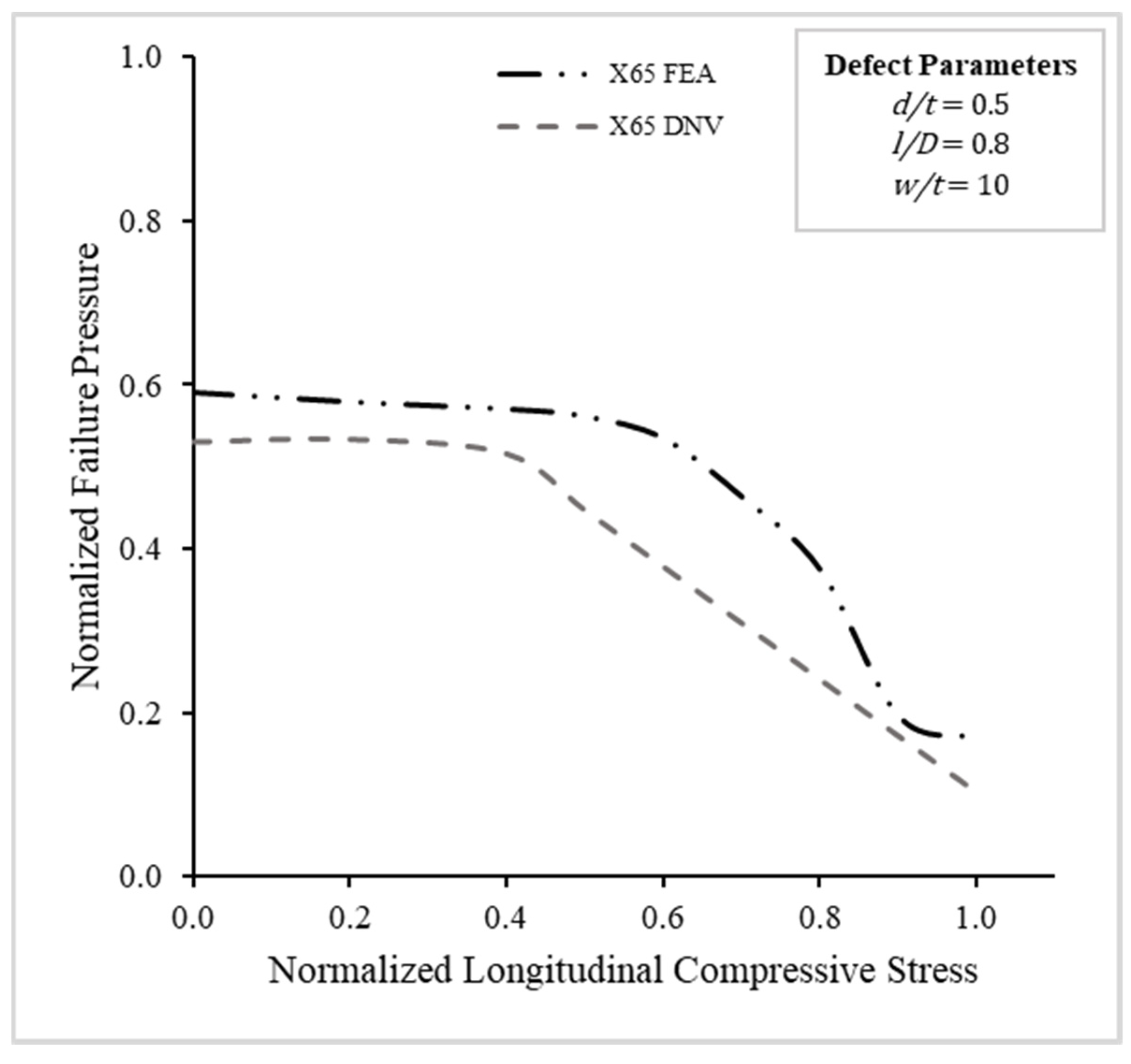
Figure 9 shows the trends in the effects of combined internal pressure and longitudinal compressive stress on the failure pressure obtained from the FEA and DNV calculations of SDOFAT27 to SDOFAT33. Low longitudinal compressive stress (<0.4 ${\sigma }_c/{\sigma }_y$) had a nominal effect on the failure pressure of the corroded pipe in both FEA and DNV. Beyond 0.4 ${\sigma }_c/{\sigma }_y$, the detrimental effect of combined loads on failure pressure was observable in both trendlines. The failure pressure in the DNV trendline decreased linearly, whereas the failure pressure in the FEA trendline decreased exponentially and then plateaued when the external load was over 0.9 ${\sigma }_c/{\sigma }_y$. 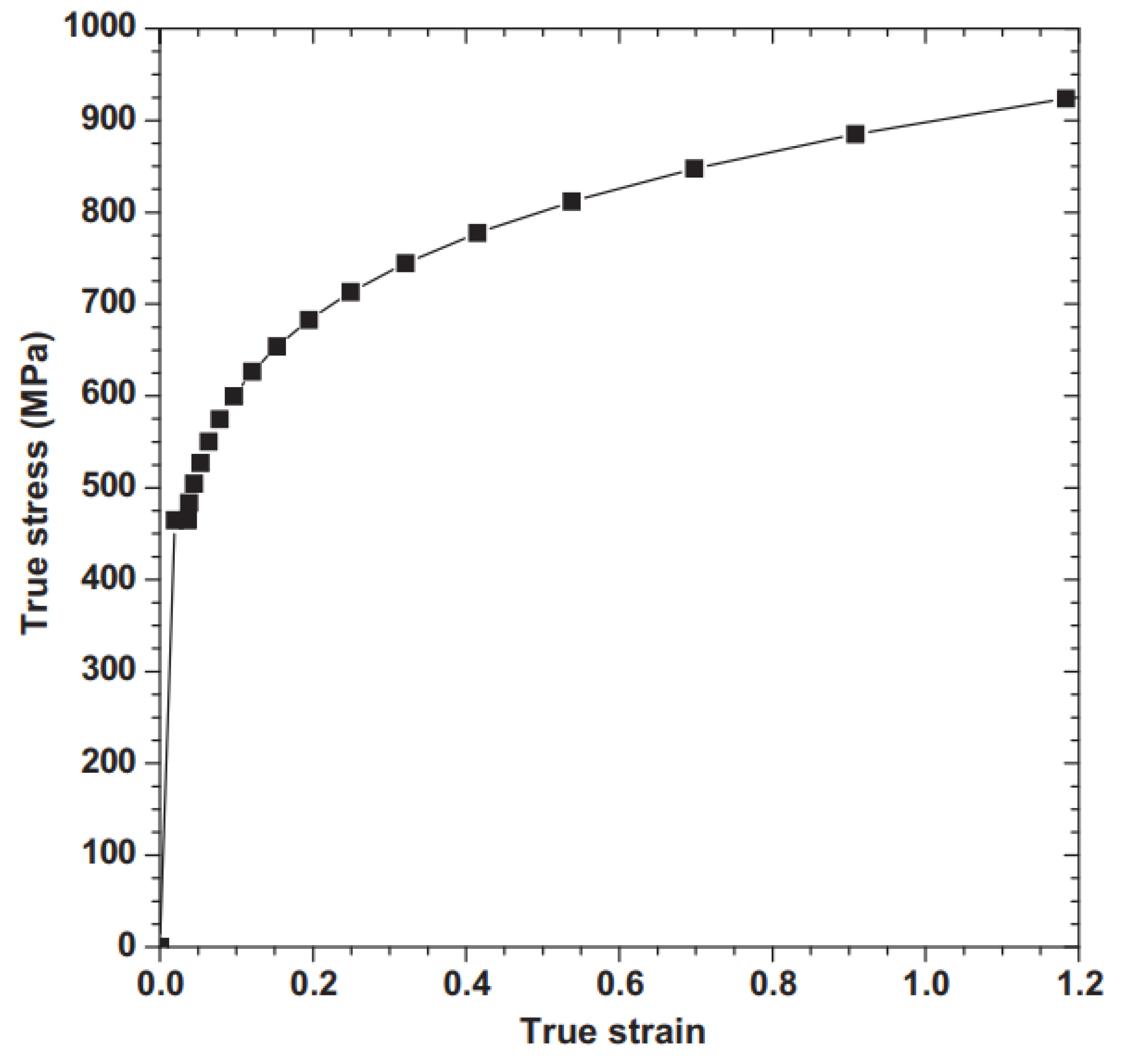The inverse sigmoid shape of the FEA trendline can be explained by the change from elastic deformation to plastic deformation. In elastic deformation, the mechanical work of the external load was converted into elastic strain energy, and, consequently, decreased the failure pressure. By contrast, in plastic deformation, the mechanical work was converted into other types of internal energy absorbed by the steel, such as lattice distortion, dislocation movement, etc. [4]. Therefore, the DNV corrosion assessment method is conservative in its predictions when used for assessing the combined load of internal pressure and longitudinal compressive stress. The mean average percentage difference between the FEA predictions and DNV predictions was 31.33%.

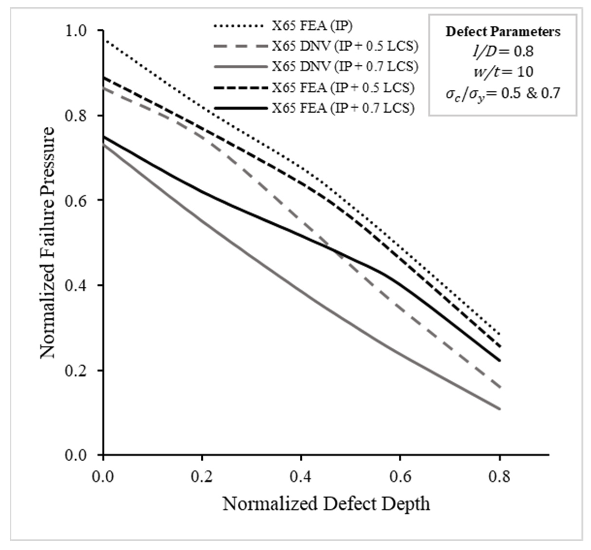
The effect of corrosion defect depth on failure pressure when subjected to combined loads is shown in Figure 10. Longitudinal compressive stresses (LCSs) of 0.5 ${\sigma }_c/{\sigma }_y$ and 0.8 ${\sigma }_c/{\sigma }_y$ were considered to investigate the effects of different external loads on top of defect geometric changes on the failure pressure of X65 pipelines with single corrosion. All the trendlines show the detrimental effects of corrosion defect depth on the failure pressure of corroded pipelines subjected to internal pressure only, as well as on the internal pressure and longitudinal compressive stress. The thinning of the pipe wall thickness decreased the failure pressure, which can be attributed to the reduced ability to resist hoop stress that developed from the internal pressure [1,39,40]. The failure pressure of the X65 FEA (IP + 0.8 LCS) was near zero when the defect depth was 0.8 d/t, due to buckling failure. It is known that longitudinal compressive stress causes buckling failure, especially in corroded pipelines [41] and higher-grade steel. High-toughness steels are more prone to buckling failure due to lower critical compressive stress [42]. The DNV assessment method underestimated the failure pressure when compared with the FEA, with the mean average percentage difference for IP + 0.5 LCS trendlines being 27.04%.

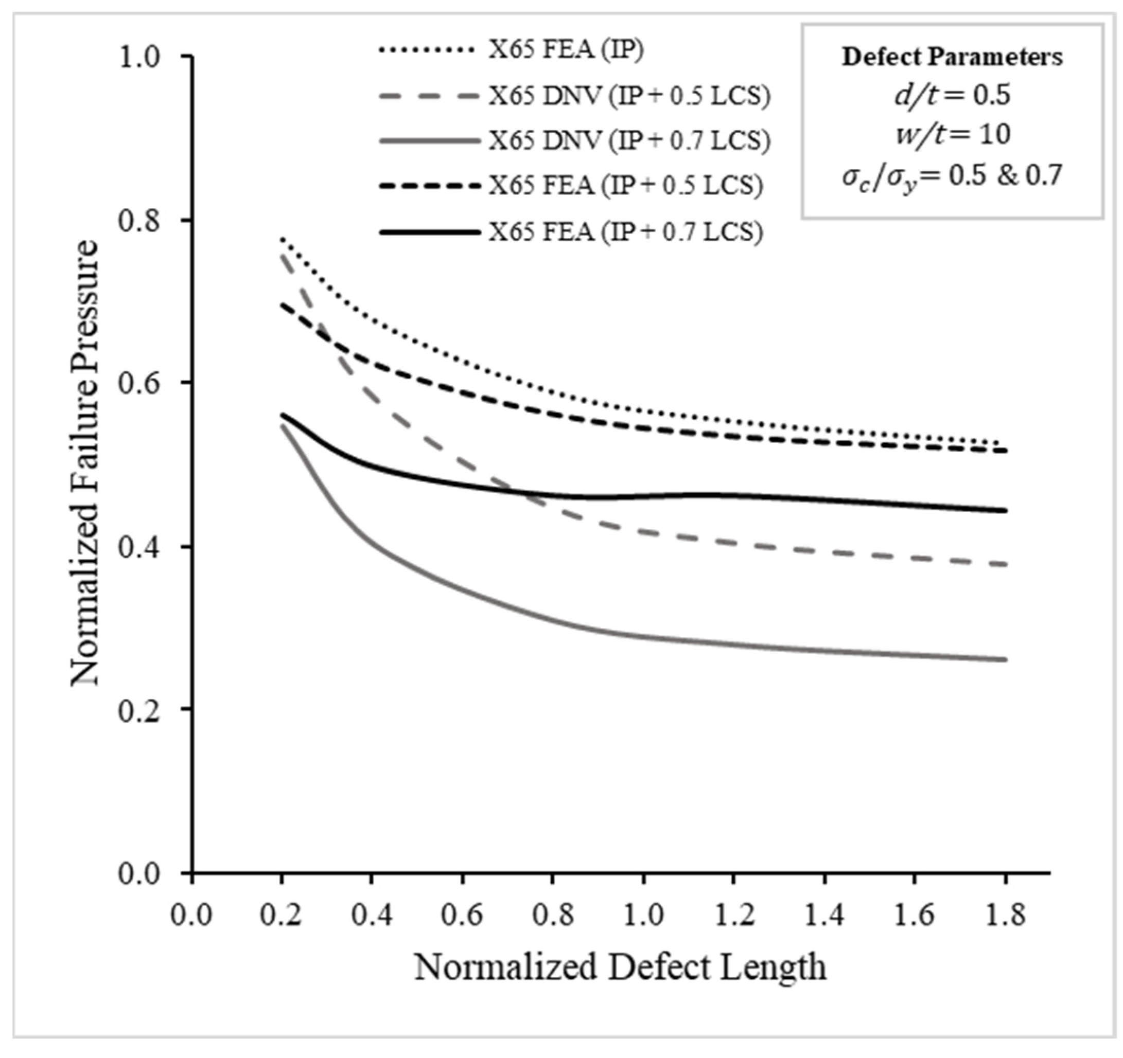
Figure 11 shows the trends in the corrosion defect length against the failure pressure of the corroded pipeline subjected to combined load. An increase in the corrosion defect length reduced the failure pressure up until a critical point, when the normalized defect length was 1.2 l/D, beyond which the failure pressure stayed the same. The result was consistent with past research on for internal pressure only and combined loads [37,39]. The mean average percentage difference between the X65 FEA (IP + 0.5 LCS) predictions and the predictions from its DNV counterpart was 18.73%, which shows the conservative character of the estimations using the DNV assessment method.

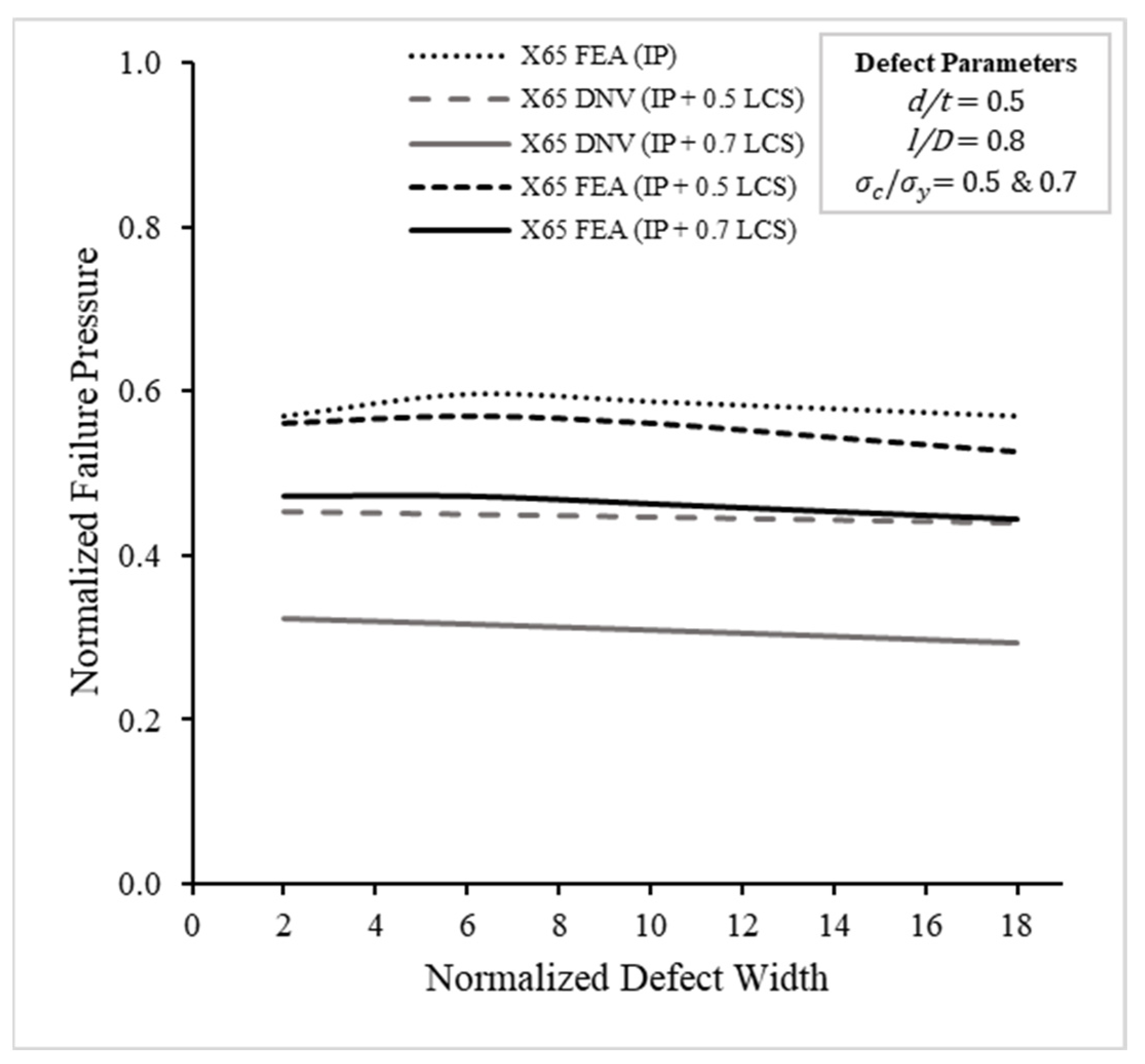
The effect of the corrosion defect width on the failure pressure subjected to internal pressure and longitudinal compressive stress is shown in Figure 12. The general trends pointed to a slight decrease in the failure pressure when the corrosion defect width increased in the circumferential direction, except for the trendline of X65 FEA (IP + 0.8 LCS). The DNV assessment method underestimated the failure pressure when compared with the FEA; the mean average percentage difference for the IP + 0.5 LCS trendlines was 23.6%.

The application of longitudinal compressive stress further exacerbated the decrease in failure pressure, as seen through the comparison of the X65 FEA (IP), X65 FEA (IP + 0.5 LCS), and X65 FEA (IP + 0.8 LCS) trendlines. The difference between no longitudinal compressive stress (LCS), 0.5 ${\sigma }_c/{\sigma }_y$, and 0.8 ${\sigma }_c/{\sigma }_y$ is evident in all three figures. For a normalized defect depth of 0.5 d/t, the normalized defect length of 0.8 l/D, and the normalized defect width of 10 w/t, the percentage difference between the FEA results with no LCS and 0.8 ${\sigma }_c/{\sigma }_y$ is 37.29%, which is a larger difference in failure pressure compared with the percentage difference between no LCS and 0.5 ${\sigma }_c/{\sigma }_y$ (5.08%). This large difference in the decrease in failure pressure over a small increment of LCS was due to the different rate of change, as seen in Figure 7. The rate of change for the failure pressure in the beginning (0 to 0.4 ${\sigma }_c/{\sigma }_y$) was less than −0.09; at 0.5 ${\sigma }_c/{\sigma }_y$ the rate of change was −0.27; and at 0.8 ${\sigma }_c/{\sigma }_y$ the rate of change was at its highest (−1.78). The X65 FEA (IP + 0.8 LCS) trendlines in Figure 11 and Figure 12 both show sudden decreases in failure pressure followed by plateaus when the normalized defect length was 0.8 l/D and the normalized defect width was 10 w/t, respectively. Due to changes from elastic deformation to plastic deformation, teetering near buckling failure, the decrease in failure pressure exhibits an inverse sigmoid-shaped trend, as in Figure 9.

3.2. Further Finite Element Analysis

The preliminary study from the SDOFAT tests proved the conservatism of the DNV assessment method in predicting the failure pressure of corroded pipes when subjected to both internal pressure and longitudinal compressive stress. The previous analyses gave insights into the selection of appropriate parametric bounds for the corrosion defect geometry and longitudinal compressive stress. This study highlighted the significance of the corrosion defect depth ranging from 0.2 d/t to 0.8 d/t. The defect length influenced the failure pressure from 0.2 l/D to 1.2 l/D, until the critical defect length of 1.2 l/D, where the failure pressure plateaued. On the other hand, the preliminary FEA showed that the defect width had minimal influence on the failure pressure; the longitudinal compressive stress ranged from 0.2 ${\sigma }_c/{\sigma }_y$ to 0.7 ${\sigma }_c/{\sigma }_y.$ Longitudinal compressive stresses beyond 0.8 ${\sigma }_c/{\sigma }_y$ were not considered, as the pipeline was at risk of buckling failure and would normally be replaced or changed when the longitudinal compressive stress exceeded 0.6 ${\sigma }_c/{\sigma }_y$. Thus, only longitudinal compressive stress ranging from 0.2 ${\sigma }_c/{\sigma }_y$ to 0.7 ${\sigma }_c/{\sigma }_y$ was considered in further work and the defect width parameter was excluded from further FEAs.

Table 9. FEA on corroded pipeline with single corrosion defect subjected to internal pressure and longitudinal compressive stress.

d/t	l/D	${\mathit{\sigma }}_{\mathit{c}}/{\mathit{\sigma }}_{\mathit{y}}$
		0.2	0.4	0.5	0.6	0.7
0.2	0.2	0.88	0.85	0.79	0.74	0.61
	0.4	0.85	0.82	0.77	0.70	0.59
	0.6	0.84	0.79	0.75	0.68	0.56
	0.8	0.83	0.78	0.74	0.66	0.54
	1.2	0.81	0.77	0.73	0.65	0.53
0.4	0.2	0.80	0.76	0.71	0.67	0.59
	0.4	0.75	0.71	0.68	0.62	0.54
	0.6	0.70	0.68	0.65	0.61	0.53
	0.8	0.68	0.66	0.64	0.60	0.52
	1.2	0.65	0.63	0.62	0.59	0.52
0.5	0.2	0.77	0.73	0.69	0.64	0.56
	0.4	0.67	0.65	0.62	0.58	0.50
	0.6	0.61	0.60	0.58	0.54	0.47
	0.8	0.58	0.57	0.56	0.53	0.46
	1.2	0.55	0.54	0.53	0.52	0.46
0.6	0.2	0.72	0.69	0.66	0.61	0.53
	0.4	0.59	0.57	0.55	0.52	0.45
	0.6	0.53	0.51	0.49	0.47	0.41
	0.8	0.49	0.47	0.46	0.45	0.40
	1.2	0.45	0.45	0.44	0.43	0.39
0.8	0.2	0.58	0.56	0.55	0.52	0.44
	0.4	0.39	0.37	0.36	0.34	0.28
	0.6	0.32	0.30	0.29	0.28	0.24
	0.8	0.28	0.27	0.26	0.25	0.22
	1.2	0.25	0.24	0.24	0.23	0.21

lists the failure pressure values from the FEA predictions of corrosion defect, with full factorial defect geometries according to selected parametric bounds.

3.3. Development of New Assessment Equation Using ANN

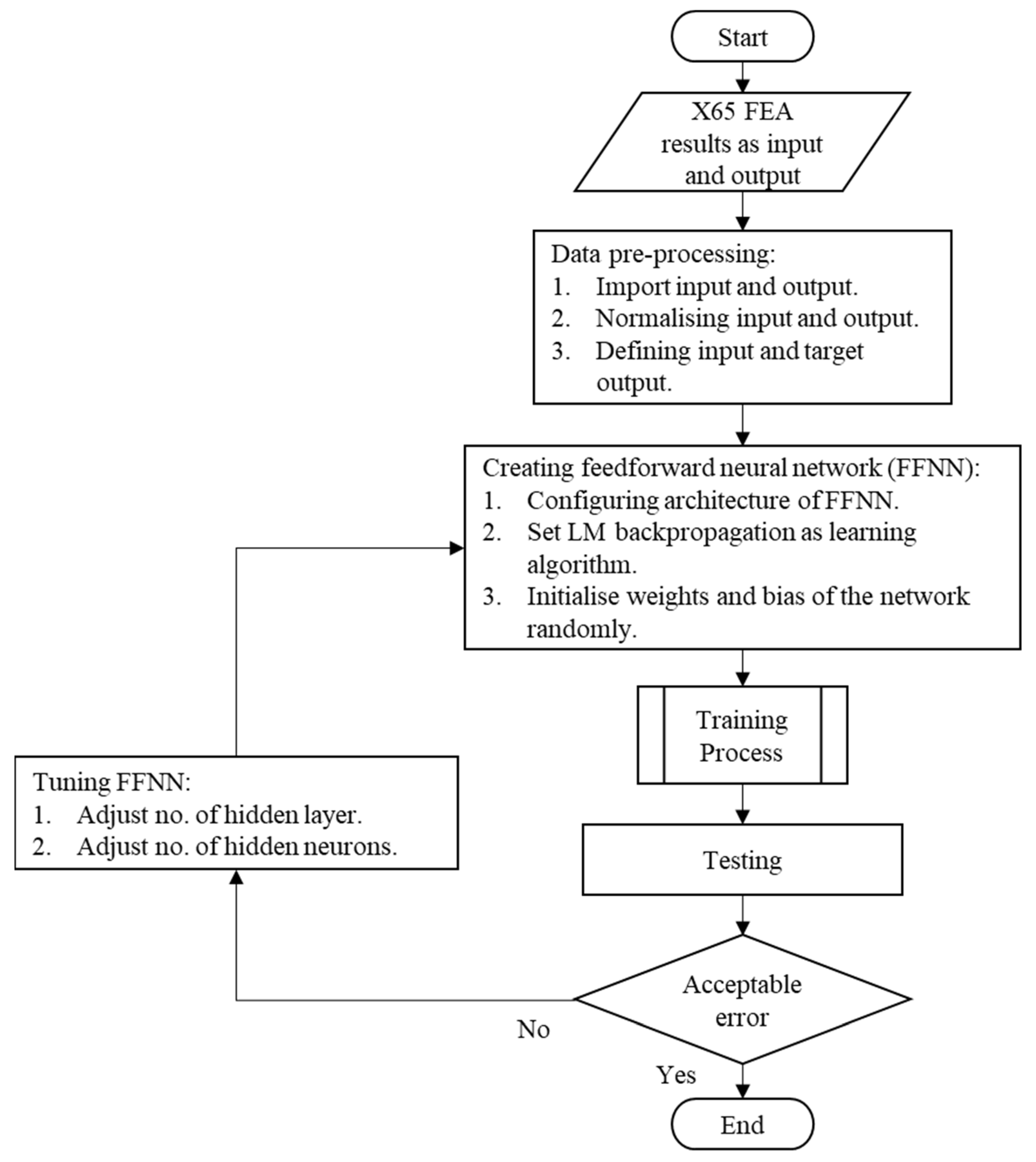
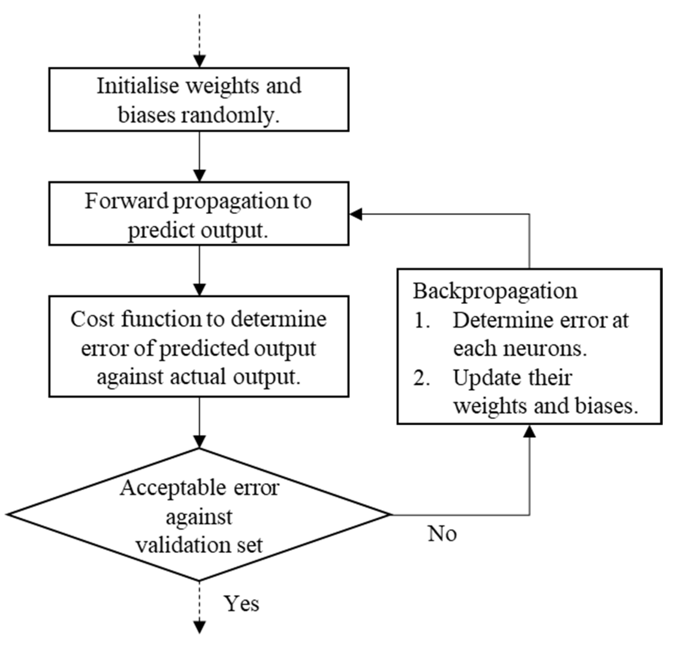
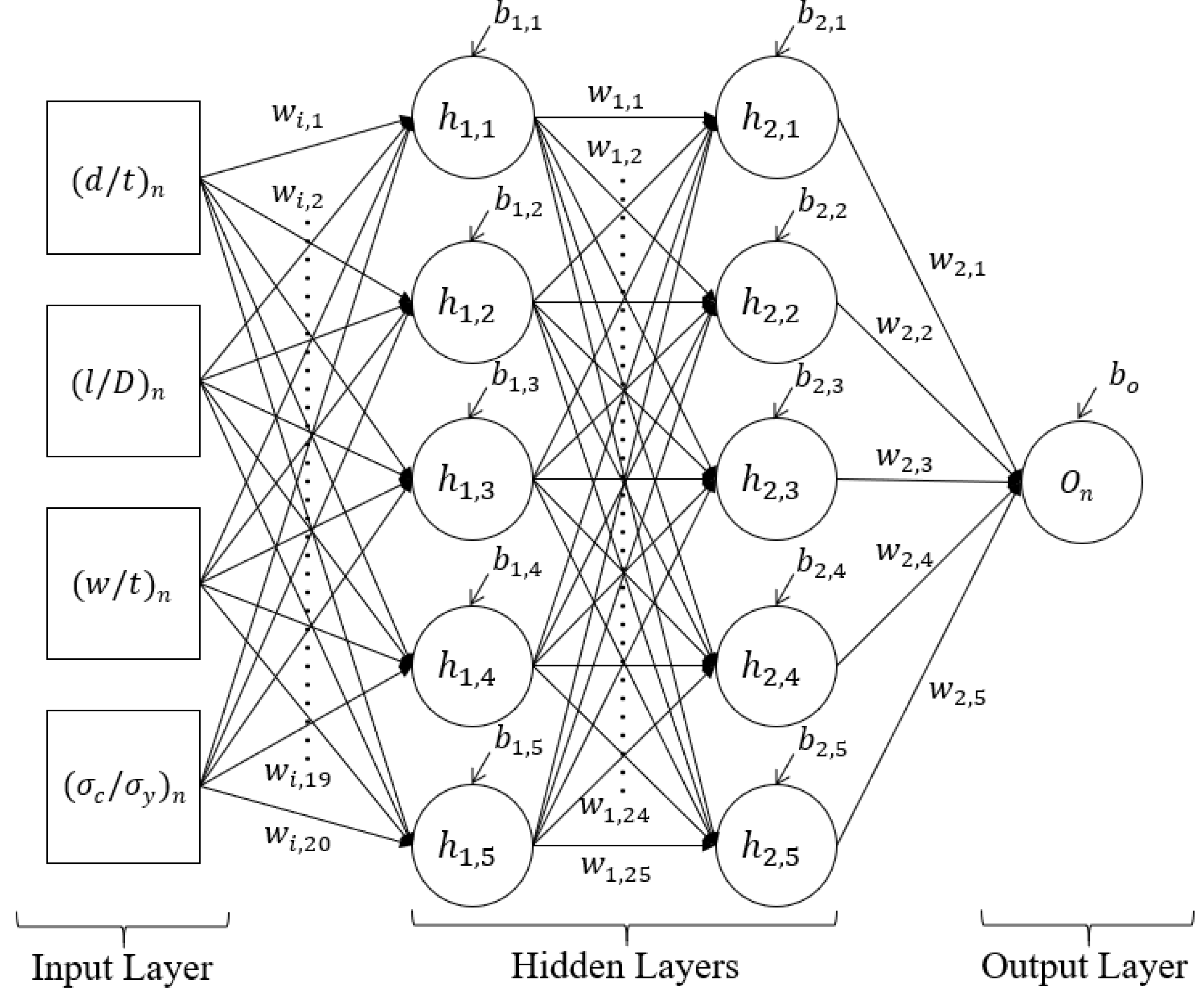
MathWorks MATLAB R2019b was used to develop the ANN model to predict the failure pressure of the corroded pipeline with longitudinal interacting defects. The architecture of the ANN was based on a feedforward neural network (FFNN) with a Levenberg–Marquardt backpropagation training algorithm. The three inputs of the ANN model were normalized corrosion defect depth, $d/t$, normalized corrosion defect length, $l/D$, and normalized axial compressive stress, ${\sigma }_c/{\sigma }_y$. The target output with which the ANN model was trained was the normalized failure pressure, $P_f/P_i$. The network had two hidden layers, with five hidden neurons in each hidden layer. The number of hidden layers and hidden neurons was pruned through trial and error to find the best-performing neural network configuration. A hyperbolic tangent sigmoid transfer function was applied in both hidden layers and a linear transfer function is applied in the output layer.

All 125 sets of data from the further FEA were used for the development of the ANN model and to train the feedforward neural network created. The trained neural network could be expressed in mathematical form to develop a new assessment method to predict the failure pressure of the single-defect corroded pipeline subjected to axial compressive stress. The input and output neurons were normalized $d/t$, $l/D$, ${\sigma }_c/{\sigma }_y$ and $P_f/P_i$ to be in the range of −1 to 1. The normalization of the values, as expressed in Equation (5), unified the values going into the neurons and ultimately improved the predictions of the ANN model:

$${\left(y\right)}_n=\frac{\left(y_{max}-y_{min}\right)\left(x-x_{min}\right) }{\left(x_{max}-x_{min}\right)}+y_{min}$$

(5)

where $y$ is the normalization value ranging from −1 to 1 and $x$ is the denormalization value, with ranges according to its dataset.

The ANN was made of interconnected input neurons, hidden neurons, and output neurons as illustrated in Figure 13. The values of the links between the neurons were weights that either amplified or dampened the input value. The value $w_{i,x}$ denotes weights linking the input layer to hidden layer 1, $h_{1,x}$. The value $w_{1,x}$ denotes weights linking $h_{1,x}$ to hidden layer 2,$h_{2,x}$. The value $w_{2,x}$ denotes weights linking the $h_{2,x}$ to output layer. The biases ($b_{x,x}$) are the constant non-zero values of hidden neurons that were then summed with the product of inputs and weights. The result was then transferred through the transfer function of the neuron as its output. Linear transfer functions were used in the neurons in the input layer and output layer; hyperbolic-tangent sigmoid transfer functions were used in the neurons in the hidden layers.

The connections between the input, output, hidden neurons, and its weights and biases can be expressed in the mathematical form of Equations (6)–(8). After training the ANN with all the datasets, the weights and biases were adjusted for output predictions with the lowest error. The weights and biases of the network were extracted and used in Equations (6)–(8), and they are expressed as follows:

$$\left[\begin{array}{c}{h}_{1,1}\\ h_{1,2}\\ h_{1,3}\\ h_{1,4}\\ h_{1,5}\end{array}\right]=\left[\begin{array}{ccc}0.7632& -0.0274& -0.0574\\ -0.6316& -0.0695& 1.0786\\ 0.4025& -2.0078& -0.394\\ -0.4175& -1.0692& 0.4495\\ -0.2339& -0.2975& -0.4053\end{array}\right]\left[\begin{array}{c}{\left(d/t\right)}_n\\ {\left(l/D\right)}_n\\ {\left({\sigma }_c/{\sigma }_y\right)}_n\end{array}\right]+\left[\begin{array}{c}-0.0301\\ -1.7023\\ -2.7257\\ -0.5119\\ -1.9501\end{array}\right]$$

(6)

$$\left[\begin{array}{c}{h}_{2,1}\\ h_{2,2}\\ h_{2,3}\\ h_{2,4}\\ h_{2,5}\end{array}\right]=\left[\begin{array}{ccccc}0.7682& 0.496& -0.2244& 0.2622& 1.5642\\ 0.9013& -0.0597& 0.3389& 0.8929& -1.4931\\ 0.5611& -2.0144& 0.7029& -0.7315& 8.7401\\ 0.3936& 0.3176& -0.1817& 0.0686& -0.1516\\ -0.9168& -0.1345& -0.3502& -0.7165& -0.6376\end{array}\right]\left[\begin{array}{c}a\left(h_{1,1}\right)\\ a\left(h_{1,2}\right)\\ a\left(h_{1,3}\right)\\ a\left(h_{1,4}\right)\\ a\left(h_{1,5}\right)\end{array}\right]+\left[\begin{array}{c}1.6792\\ -0.5094\\ 5.7444\\ -0.6877\\ -1.5873\end{array}\right]$$

(7)

$$\left[O_n\right]=f\left\{\left[\begin{array}{ccccc}9.6294& 3.7833& -0.428& -20.4331& 6.7248\end{array}\right]\left[\begin{array}{c}a\left(h_{2,1}\right)\\ a\left(h_{2,2}\right)\\ a\left(h_{2,3}\right)\\ a\left(h_{2,4}\right)\\ a\left(h_{2,5}\right)\end{array}\right]+\left[-10.4688\right]\right\}$$

(8)

where $a\left(x\right)$ is hyperbolic tangent sigmoid transfer function

$$a\left(x\right)=\frac{2}{\left(1+e^{-2x}\right)-1} \mathrm{or} \tan \mathrm{h}\left(x\right)$$

(9)

and $f\left(x\right)$ is linear transfer function

$$f\left(x\right)=x$$

(10)

Equations (6)–(8) were developed based on the dataset used to train the neural network. Therefore, they are applicable for parameters within the range of the dataset. However, the equations were shown to be flexible enough to assess the parameters near the range of the dataset from which they were developed, when their performance was tested.

3.4. Development of New Assessment Equation Using ANN

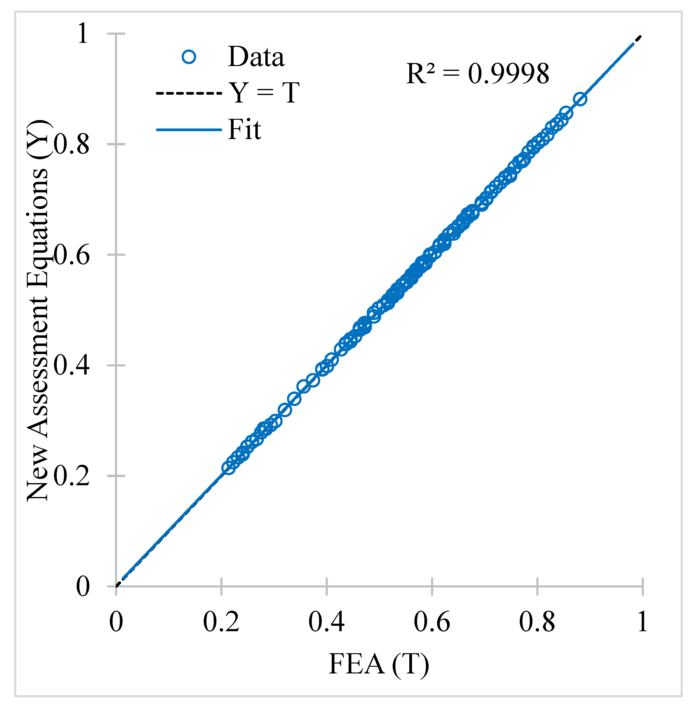
The R² value of the ANN-based corrosion assessment equation was 0.9998, which showed a good correlation between the predictions from the new assessment equation and the FEA results of the single-defect corroded pipe subjected to combined loads of internal pressure and longitudinal compressive stress. When the equations’ predictions were evaluated against the FEA results, the percentage error ranged from −1.16% to 1.78%, with a standard deviation of 0.49. The percentage errors were within acceptable limits (<5%) and the standard deviation of the new assessment equations was lower than in the literature [16]. Figure 14 illustrates the performance of the new assessment equation in a regression plot. The new assessment equations were very accurate, with MSE of 0.00000533 and MAE of 0.00191.

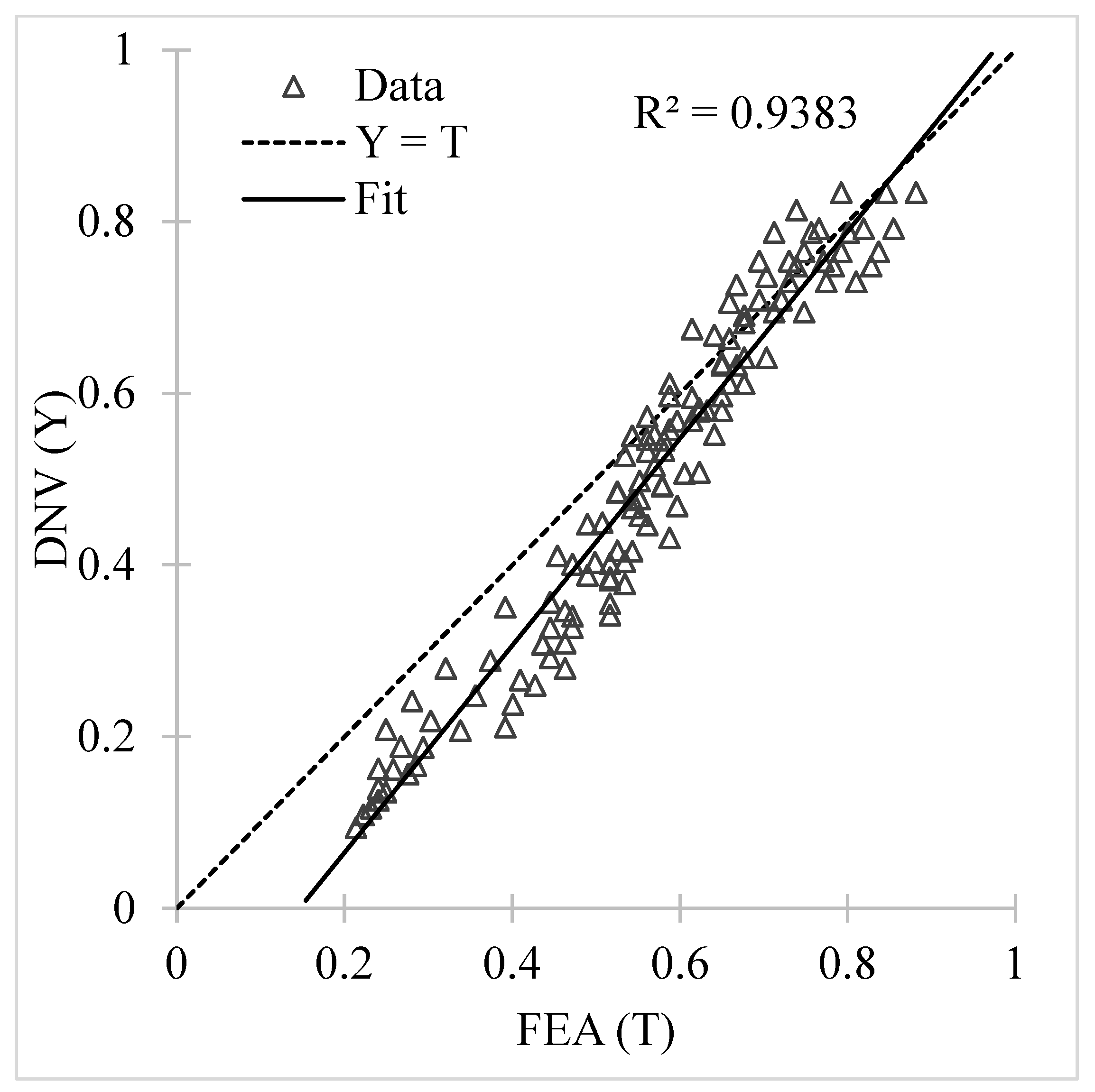
By contrast, the R² value of the DNV assessment method, when evaluated against the FEA results, was 0.9383, with a standard deviation of 15.59. The error percentage between the DNV predictions and the FEA results ranged from −56.03% to 10.56%. Figure 15 shows the regression plot of the DNV predictions and FEA results. The DNV assessment method had a MSE of 0.00739 and MAE of 0.0717. The DNV assessment method tended to be conservative in its prediction when the failure pressure was low, as observed in the regression plot, with percentage differences up to −56.03%. Its standard deviation was far higher than the new assessment equation, by 15.1, which shows the inaccuracy of the DNV method. This conservatism leads to downtime and economic costs in the form of premature maintenance and shutdowns of pipelines.

To ensure the reliability of the new assessment equations, burst test results and a new, unseen FEA dataset were used to validate the method and determine its performance.

Table 10. Failure pressure from burst tests compared with failure pressure predicted by new assessment equations.

Specimen	Failure Pressure from Burst Tests (MPa)	Failure Pressure Predicted in FEA (MPa)	Absolute Percentage Difference (%)
Validation for internal pressure only.
LD	19.80	19.97	0.86
LF	15.00	19.87	33.13
No. 61	24.11	25.43	5.47
No. 62	21.76	21.81	0.23
No. 63	17.15	16.37	4.55
Validation for internal pressure and longitudinal compressive stress.
Test 5	28.60	25.70	10.14
Test 6	28.70	25.70	10.45

shows the burst tests used to validate the FEA previously and

Table 11. Normalized failure pressure prediction using FEA and prediction made by new assessment equations on unseen dataset.

Defect Parameters		External Load	Normalized Failure Pressure		Difference
d/t	l/D	${\sigma }_c/{\sigma }_y$	FEA	New Equations	%
0.1	0.3	0.3	0.8903	0.9283	4.27
0.1	0.3	0.6	0.7300	0.7513	2.91
0.1	0.7	0.3	0.8814	0.8590	−2.54
0.1	0.9	0.3	0.8725	0.8558	−1.92
0.2	0.5	0.32	0.8280	0.8283	0.04
0.2	0.7	0.45	0.7567	0.7689	1.61
0.2	1.15	0.3	0.7924	0.7969	0.57
0.2	1.15	0.6	0.6766	0.6518	−3.66
0.3	0.3	0.3	0.7924	0.8217	3.70
0.3	0.3	0.6	0.6499	0.6846	5.34
0.35	0.7	0.6	0.6232	0.6251	0.30
0.35	1.1	0.35	0.6855	0.6871	0.23
0.35	1.1	0.6	0.6143	0.6152	0.14
0.4	0.5	0.32	0.7122	0.7117	−0.7
0.45	0.7	0.6	0.5698	0.5710	0.22
0.45	1.1	0.6	0.5876	0.5910	0.58
0.55	0.3	0.6	0.5787	0.5841	0.94
0.55	0.5	0.35	0.5787	0.5891	1.80
0.55	1.15	0.6	0.4719	0.4757	0.82
0.7	0.5	0.25	0.4540	0.4453	−1.92
0.7	0.7	0.35	0.3917	0.3875	01.07
0.8	0.2	0.5	0.5609	0.5509	−1.78
0.8	0.3	0.35	0.4630	0.4525	−2.25
0.8	0.3	0.6	0.4184	0.4060	−2.98
0.8	0.7	0.25	0.2938	0.2929	−0.30
0.8	0.7	0.5	0.2760	0.2743	−0.62
0.8	0.7	0.6	0.2582	0.2634	2.01
0.8	1.1	0.25	0.2582	0.2539	−1.66
0.8	1.1	0.35	0.2493	0.2475	−0.71
0.8	1.1	0.5	0.2404	0.2419	0.63

includes the parameters and FEA results of the 30 sets of unseen data. From Table 10, the absolute difference between the failure pressure of burst tests and the predictions by new assessment equations ranged from 0.23% to 33.13%. In Table 11, the new assessment equations are accurate in their estimations of the normalized failure pressure with percentage differences between the FEA and the new equations ranging from −3.66% to 5.34%.

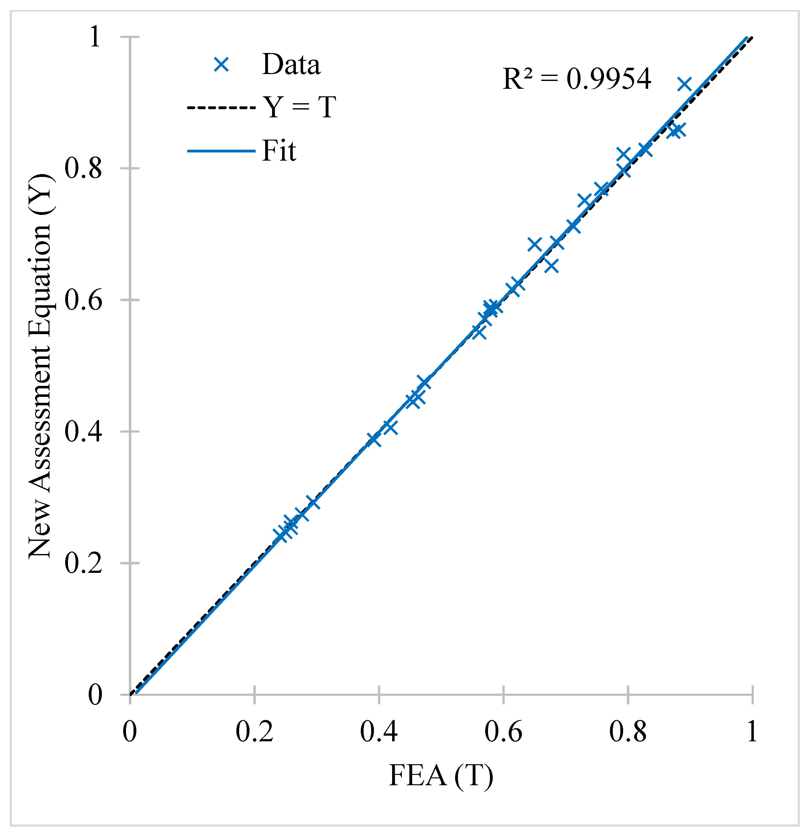
The R² value of the new assessment equations when tested against the unseen dataset was 0.9954, which indicated a good correlation, as shown in Figure 16. The new assessment equations had a MSE of 0.000207 and a MAE of 0.00982.

3.5. Recommendations for New Corrosion Assessment Equation

ANNs rely heavily on the quality of input data to produce accurate and precise predictions. Therefore, more inclusive FEAs could be designed to improve the robustness of the new corrosion assessment equations. Nevertheless, the newly developed assessment equation was more accurate than the DNV, as it was based on an FEM that employs true UTS as the failure criterion. The equation could be used in spreadsheets to predict accurate failure pressure in a short time. However, it is advised to use the equation in conjunction with established standards for corrosion assessment, as the ANN-based assessment equation is based on the material properties, corrosion geometric parameters, and load applications considered in this work. Comprehensive, risk-based integrity management that considers all perspectives is recommended to ensure fitness-of-service.

4. Conclusions

A FEM was developed to simulate single-defect corrosion on a corroded pipeline to predict the failure pressure when the pipeline was subjected to combined loads of internal pressure and longitudinal compressive stress. The true stress–strain values and true UTS of the pipe’s material properties were employed as the FEM failure criteria instead of the engineering values. The FEM was validated by the results of burst tests from past research. From the preliminary FEA study, the defect depth and defect length (up to a critical level) had a significant influence on the failure pressure, while the defect width only had a considerable effect on the failure pressure when the longitudinal compressive stress was greater than 0.7 ${\sigma }_c/{\sigma }_y$. The appropriate ranges for the corrosion geometric parameters and load applications were then chosen for further comprehensive FEAs. The FEA results were used as an input database to train the ANN for the development of a new assessment equation. The weights and biases of the network were extracted to develop an ANN-based corrosion assessment equation, and its performance was compared with the DNV assessment method and validated with an unseen dataset. According to the comparison, the predictions made with the DNV method were more conservative than the predictions based on the new assessment equations. The predictions from the new equations had an R² value of 0.9998, with percentage errors ranging from −1.16% to 1.78%. It is recommended to employ the newly developed assessment equation as a supplement to established standards for the rigorous assessment of corroded pipelines subjected to combined loads.

References

1. Han, C.J.; Zhang, H.; Zhang, J. Failure Pressure Analysis of the Pipe with Inner Corrosion Defects by FEM. Int. J. Electrochem. Sci. 2016, 11, 5046–5062. [Google Scholar] [CrossRef]
2. Cerit, M. Corrosion Pit-Induced Stress Concentration in Spherical Pressure Vessel. Thin Walled Struct. 2019, 136, 106–112. [Google Scholar] [CrossRef]
3. Grigory, S.C.; Smith, M.Q. Residual Strength of 48-Inch Diameter Corroded Pipe Determined by Full Scale Combined Loading Experiments. In Proceedings of the International Pipeline Conference, IPC, Calgary, AB, Canada, 9–13 June 1996; pp. 377–386. [Google Scholar] [CrossRef]
4. Xu, L.Y.; Cheng, Y.F. Reliability and Failure Pressure Prediction of Various Grades of Pipeline Steel in the Presence of Corrosion Defects and Pre-Strain. Int. J. Press. Vessel. Pip. 2012, 89, 75–84. [Google Scholar] [CrossRef]
5. Seyfipour, I.; Bahaari, M.R. Analytical Study of Subsea Pipeline Behaviour Subjected to Axial Load in Free-Span Location. J. Mar. Eng. Technol. 2021, 20, 151–158. [Google Scholar] [CrossRef]
6. Bjørnøy, O.H.; Sigurdsson, G.; Cramer, E. Residual Strength of Corroded Pipelines, DNV Test Results. In Proceedings of the Tenth International Offshore and Polar Engineering Conference, Seattle, WA, USA, 28 May–2 June 2000. [Google Scholar]
7. Chauhan, V.; Swankie, T.; Espiner, R.; Wood, I. Developments in methods for assessing the remaining strength of corroded pipelines. In Proceedings of the CORROSION 2009, Atlanta, GA, USA, 22–26 March 2009; NACE International: Houston, TX, USA, 2009. [Google Scholar]
8. Barbosa, A.; Teixeira, A.; Soares, C.G.; Li, M.; Kang, J.; Sun, L.; Wang, M.; Garbatov, Y. Strength analysis of corroded pipelines subjected to internal pressure and bending moment. In Proceedings of the Progress in the Analysis and Design of Marine Structures, Lisbon, Portugal, 8–10 May 2017; CRC Press: Boca Raton, FL, USA, 2017; pp. 803–812. [Google Scholar] [CrossRef]
9. Belachew, C.T.; Ismail, M.C.; Karuppanan, S. Burst Strength Analysis of Corroded Pipelines by Finite Element Method. J. Appl. Sci. 2011, 11, 1845–1850. [Google Scholar] [CrossRef]
10. Smith, M.Q.; Grigory, S.C. New procedures for the residual strength assessment of corroded pipe subjected to combined loads. In Proceedings of the International Pipeline Conference, IPC, Calgary, AB, Canada, 9–14 June 1996; pp. 387–400. [Google Scholar] [CrossRef]
11. Roy, S.; Grigory, S.; Smith, M.; Kanninen, M.F.; Anderson, M. Numerical Simulations of Full- Scale Corroded Pipe Tests with Combined Loading. J. Press. Vessel Technol. Trans. ASME 1997, 119, 457–466. [Google Scholar] [CrossRef]
12. Mohd, M.H.; Lee, B.J.; Cui, Y.; Paik, J.K. Residual Strength of Corroded Subsea Pipelines Subject to Combined Internal Pressure and Bending Moment. Ships Offshore Struct. 2015, 10, 554–564. [Google Scholar] [CrossRef]
13. Bruère, V.M.; Bouchonneau, N.; Motta, R.S.; Afonso, S.M.B.; Willmersdorf, R.B.; Lyra, P.R.M.; Torres, J.V.S.; De Andrade, E.Q.; Cunha, D.J.S. Failure Pressure Prediction of Corroded Pipes under Combined Internal Pressure and Axial Compressive Force. J. Braz. Soc. Mech. Sci. Eng. 2019, 41, 1–10. [Google Scholar] [CrossRef]
14. Netto, T.A.; Ferraz, U.S.; Estefen, S.F. The Effect of Corrosion Defects on the Burst Pressure of Pipelines. J. Constr. Steel Res. 2005, 61, 1185–1204. [Google Scholar] [CrossRef]
15. Fahed, M.; Barsoum, I.; Alfantazi, A.; Islam, M.D. Burst Pressure Prediction of Pipes with Internal Corrosion Defects. J. Press. Vessel Technol. 2020, 142, 031801. [Google Scholar] [CrossRef]
16. Arumugam, T.; Karuppanan, S.; Ovinis, M. Finite Element Analyses of Corroded Pipeline with Single Defect Subjected to Internal Pressure and Axial Compressive Stress. Mar. Struct. 2020, 72, 102746. [Google Scholar] [CrossRef]
17. Silva, R.; Guerreiro, J.N.C.; Loula, A. A Study of Pipe Interacting Corrosion Defects Using the FEM and Neural Networks. Adv. Eng. Softw. 2007, 38, 868–875. [Google Scholar] [CrossRef]
18. Xu, W.-Z.; Li, C.B.; Choung, J.; Lee, J.-M. Corroded Pipeline Failure Analysis Using Artificial Neural Network Scheme. Adv. Eng. Softw. 2017, 112, 255–266. [Google Scholar] [CrossRef]
19. Lu, L.; Liang, L. Numerical Investigation of Corroded Middle-High Strength Pipeline Subjected to Combined Internal Pressure and Axial Compressive Loading. Energy Sci. Eng. 2021, 9, 798–811. [Google Scholar] [CrossRef]
20. Khalaj Khalajestani, M.; Bahaari, M.R.; Salehi, A.; Shahbazi, S. Predicting the Limit Pressure Capacity of Pipe Elbows Containing Single Defects. Appl. Ocean Res. 2015, 53, 15–22. [Google Scholar] [CrossRef]
21. Khalaj Khalajestani, M.; Bahaari, M.R. Investigation of Pressurized Elbows Containing Interacting Corrosion Defects. Int. J. Press. Vessel. Pip. 2014, 123–124, 77–85. [Google Scholar] [CrossRef]
22. Tohidi, S.; Sharifi, Y. Load-Carrying Capacity of Locally Corroded Steel Plate Girder Ends Using Artificial Neural Network. Thin Walled Struct. 2016, 100, 48–61. [Google Scholar] [CrossRef]
23. Kumar, S.D.V.; Karuppanan, S.; Ovinis, M. Failure Pressure Prediction of High Toughness Pipeline with a Single Corrosion Defect Subjected to Combined Loadings Using Artificial Neural Network (ANN). Metals 2021, 11, 373. [Google Scholar] [CrossRef]
24. Lo, M.; Karuppanan, S.; Ovinis, M. Failure Pressure Prediction of a Corroded Pipeline with Longitudinally Interacting Corrosion Defects Subjected to Combined Loadings Using FEM and ANN. J. Mar. Sci. Eng. 2021, 9, 281. [Google Scholar] [CrossRef]
25. Amaya-Gómez, R.; Sánchez-Silva, M.; Bastidas-Arteaga, E.; Schoefs, F.; Muñoz, F. Reliability Assessments of Corroded Pipelines Based on Internal Pressure—A Review. Eng. Fail. Anal. 2019, 98, 190–214. [Google Scholar] [CrossRef]
26. BS 7910: 2013+ A1: 2015; Guide to Methods for Assessing the Acceptability of Flaws in Metallic Structures. British Standard Institute: London, UK, 2015.
27. Kim, Y.J.; Oh, C.S. Limit Loads for Pipe Bends under Combined Pressure and In-Plane Bending Based on Finite Element Limit Analysis. Int. J. Press. Vessel. Pip. 2006, 83, 148–153. [Google Scholar] [CrossRef]
28. Al-Owaisi, S.S.; Becker, A.A.; Sun, W. Analysis of Shape and Location Effects of Closely Spaced Metal Loss Defects in Pressurised Pipes. Eng. Fail. Anal. 2016, 68, 172–186. [Google Scholar] [CrossRef]
29. Baek, J.H.; Kim, Y.P.; Kim, W.S.; Koo, J.M.; Seok, C.S. Load Bearing Capacity of API X65 Pipe with Dent Defect under Internal Pressure and In-Plane Bending. Mater. Sci. Eng. A 2012, 540, 70–82. [Google Scholar] [CrossRef]
30. Choi, J.B.; Goo, B.K.; Kim, J.C.; Kim, Y.J.; Kim, W.S. Development of Limit Load Solutions for Corroded Gas Pipelines. Int. J. Press. Vessel. Pip. 2003, 80, 121–128. [Google Scholar] [CrossRef]
31. Kim, Y.; Kim, W.; Lee, Y.; Oh, K. The Evaluation of Failure Pressure for Corrosion Defects Within Girth or Seam Weld in Transmission Pipelines. In Proceedings of the 2004 International Pipeline Conference, Calgary, AB, Canada, 4–8 October 2004; ASMEDC: New York, NY, USA, 2004; Volume 1–3, pp. 1847–1855. [Google Scholar] [CrossRef]
32. Ma, B.; Shuai, J.; Liu, D.; Xu, K. Assessment on Failure Pressure of High Strength Pipeline with Corrosion Defects. Eng. Fail. Anal. 2013, 32, 209–219. [Google Scholar] [CrossRef]
33. Nasiri, S.; Khosravani, M.R. Machine learning in predicting mechanical behavior of additively manufactured parts. J. Mater. Res. Technol. 2021, 14, 1137–1153. [Google Scholar] [CrossRef]
34. Dhimish, M.; Holmes, V.; Mehrdadi, B.; Dales, M. Comparing Mamdani Sugeno fuzzy logic and RBF ANN network for PV fault detection. Renew. Energy 2018, 117, 257–274. [Google Scholar] [CrossRef] [Green Version]
35. Hagan, M.T.; Menhaj, M.B. Training Feedforward Networks with the Marquardt Algorithm. IEEE Trans. Neural Netw. 1994, 5, 989–993. [Google Scholar] [CrossRef]
36. Panchal, F.S.; Panchal, M. Review on Methods of Selecting Number of Hidden Nodes in Artificial Neural Network. Int. J. Comput. Sci. Mob. Comput. 2014, 3, 455–464. [Google Scholar]
37. Cosham, A.; Hopkins, P.; Macdonald, K.A. Best Practice for the Assessment of Defects in Pipelines-Corrosion. Eng. Fail. Anal. 2007, 14, 1245–1265. [Google Scholar] [CrossRef]
38. Su, C.L.; Li, X.; Zhou, J. Failure Pressure Analysis of Corroded Moderate-to-High Strength Pipelines. China Ocean Eng. 2016, 30, 69–82. [Google Scholar] [CrossRef]
39. Ahammed, M.; Melchers, R.E. Reliability Estimation of Pressurised Pipelines Subject to Localised Corrosion Defects. Int. J. Press. Vessel. Pip. 1996, 69, 267–272. [Google Scholar] [CrossRef]
40. Oh, C.K.; Kim, Y.J.; Park, C.Y. Effects of Local Wall Thinning on Net-Section Limit Loads for Pipes under Combined Pressure and Bending. Nucl. Eng. Des. 2009, 239, 261–273. [Google Scholar] [CrossRef]
41. Halima, D.; Sreekanta, D. Structural Behavior of Corroded Steel Pipes Subject to Axial Compression and Internal Pressure: Experimental Study. J. Struct. Eng. 2013, 139, 57–65. [Google Scholar] [CrossRef]
42. Li, Y.; Shuai, J.; Jin, Z.L.; Zhao, Y.T.; Xu, K. Local Buckling Failure Analysis of High-Strength Pipelines. Pet. Sci. 2017, 14, 549–559. [Google Scholar] [CrossRef] [Green Version]
Figure 1. Pitting corrosion on a pipeline.
Jmse 10 00476 g001
Figure 2. Dimension of the quarter-pipe model.
Jmse 10 00476 g002
Figure 3. Loads applied on the pipe model.
Jmse 10 00476 g003
Figure 4. Meshed pipe model and constraints imposed.
Jmse 10 00476 g004
Figure 5. True stress–strain curves of X65 steel pipe [29].
Jmse 10 00476 g005
Figure 6. Von Mises stress distribution of a failed corroded pipe with single defect.
Jmse 10 00476 g006
Figure 7. ANN development flowchart.
Jmse 10 00476 g007
Figure 8. Training process of neural network.
Jmse 10 00476 g008
Figure 9. FEA and DNV predictions of normalized failure pressure predictions versus normalized longitudinal compressive stress.
Jmse 10 00476 g009
Figure 10. FEA and DNV predictions of normalized failure pressure predictions versus normalized defect depth with 0.5 and 0.7 normalized longitudinal compressive stress.
Jmse 10 00476 g010
Figure 11. FEA and DNV predictions of normalized failure pressure predictions versus normalized defect length with 0.5 and 0.8 normalized longitudinal compressive stress.
Jmse 10 00476 g011
Figure 12. FEA and DNV predictions of normalized failure pressure predictions versus normalized defect width with 0.5 and 0.8 normalized longitudinal compressive stress.
Jmse 10 00476 g012
Figure 13. Architecture of FFNN model employed.
Jmse 10 00476 g013
Figure 14. Regression plot of normalized failure pressure predicted by the new assessment equations against FEA results.
Jmse 10 00476 g014
Figure 15. Regression plot of normalized failure pressure predicted using DNV method against FEA results.
Jmse 10 00476 g015
Figure 16. Regression plot of normalized failure pressure predicted by the new assessment equations against FEA results of unseen dataset.
Jmse 10 00476 g016