A Flexible Scheduling for Twin Yard Cranes at Container Terminals Considering Dynamic Cut-Off Time

Abstract

Yard handling is an important part of port logistics and affects the overall efficiency of the container port. The yard crane scheduling is affected by various external factors. For example, the dynamic cut-off time makes the release time of yard cranes variable, and the yard crane task arrangement will change frequently, resulting in a lot of computational time. To increase the flexibility of container yard handling, a twin yard cranes scheduling model is established considering the no-crossing constraints and the dynamic cut-off time. A joint scheduling of PSO and local re-scheduling strategy (LRPSO) is put forward to deal with the problem faster and more effectively. Small-scale and large-scale experiments are simulated to verify the performance of the proposed method. Results show that the scheduling method is more efficient.

1. Introduction

In recent years, the growing demand of shipping has had higher requirements on port handlings, and the ability of terminals to respond to emergencies needs to be improved. The container terminal yard undertakes both landing and shipping transportation. The yard crane is one of the important types of transportation equipment in the terminal yard, and its work efficiency directly affects the overall carrying efficiency of the terminal. In each container block, twin yard cranes are generally used for common rail or multi-track cooperation. Usually, the twin yard cranes are identical and move on a common rail, and collisions between them need to be avoided. This indicates that a certain safe distance should be maintained between yard cranes. In addition to internal constraints, yard cranes are often affected by other aspects, such as port congestion (Shanghai Port congestion in 2018, etc.) or sudden health conditions (2019 New Crown Epidemic, etc.) and delays in arrival time of ships. Heuermann, A. et al. [1] proposed a concept about dynamic cut-off time (cut-off time is the latest time a container may be delivered to a terminal for loading to the scheduled container vessel) and also pointed out that it is an influencing factor of yard crane handling that cannot be ignored. To improve the turnover rate of ships, the terminal yard will arrange scheduling in advance, resulting in frequent changes in the yard crane task schedule when the dynamic cut-off time occurs. If the dynamic changes increase, it is often not cost-effective to continue global scheduling. Recalculation often means a lot of time cost in a large-scale scheduling solution. In this paper, the twin yard cranes scheduling considering the dynamic cut-off time and the non-crossing constraints of yard cranes is studied. A joint scheduling of PSO and local re-scheduling strategy (LRPSO), which includes a particle swarm optimization (PSO) algorithm for initial scheduling and a local optimization strategy for re-scheduling, is proposed to shorten the computing time and improve the ability of port to respond to emergencies. Experiment results validate that the proposed method can deal with more dynamic changes at the same time and improve the flexibility of the container yard.

2. Literature Review

Improving the efficiency of container yard in port can effectively shorten the time of ships in port and improve the efficiency of port. Kemme, N. [2] pointed out that, in fact, shipping lines tend to make fewer but bigger calls with their larger vessels, i.e., increasing container volumes have to be transported in short periods of time, thus inducing increasing peak requirements in storage and handling capacity. As an important transit station for container transport at the port, the work arrangement of the container yard at the terminal is generally determined by various factors, such as the cut-off time, port resources arrangement, policy, and other factors. As an important part of the container yard, yard crane scheduling will also be affected by multiple factors.

At present, many researchers have studied the yard crane scheduling. Some researchers are concerned with the internal cross-constraint problem in multiple cranes’ cooperation. Nils, B. et al. [3] provided a classification scheme for crane scheduling problems with crane interference, and in their classification scheme, any crane scheduling problem is described by three basic elements: the terminal layout (including the available cranes), the characteristics of container moving, and an objective to be followed. Ehleiter, A. et al. [4] introduced that by considering the number of cranes, the crane scheduling can be classified as one crane, twin cranes, and triple cranes scheduling problems. Additionally, the crane scheduling problems can also be classified by considering whether the cranes can crossover each other or not. Based on the above classification ideas, this paper reviews some literature about different types of yard crane scheduling.

In the research about yard crane scheduling algorithms, some researchers proposed scheduling solution methods for different yard crane specifications. Amelie, E. et al. [5] proposed a polynomial-time algorithm to solve the twin crane scheduling problem with no-crossing constraints. Zey, L. et al. [6] solved the yard crane scheduling problem by using branch and bound algorithm for triple-crossover-cranes. Zheng, F. et al. [7] considered that the task processing time would change dynamically due to the arrangement of task retrieval and storage in the twin yard cranes scheduling problem with an inter-crane interference constraint. They used heuristics, genetic algorithms, and other methods to solve the problem. Chen, T.C. et al. [8] were concerned with the location problem of the signal transmitting station and the allocation and scheduling. They used modern network communication technology, and proposed a hybrid evolutionary algorithm IAPSO combining immune algorithm and particle swarm algorithm, which could simultaneously determine the number of signal transmission stations and the category of each station. Guo, P. et al. [9] considered the twin cranes scheduling in an automated railway container yard with a handover area, and proposed four FCFS dispatching rules to shorten the overall transportation distance of the yard crane, thereby saving the energy consumption. Lei, D. et al. [10] studied the container dispatch problem in railway container yards, proposed the concept of “dig box coefficient”, and used a multi-stage genetic algorithm considering yard crane storing containers, container sequence of the target position and the working process. Yu, M. et al. [11] proposed a variety of types of iterative-related learning particle swarm optimization (IVLPSO) to solve the quay crane scheduling and avoid the local excessively fast convergence problem of PSO.

Some researchers have also researched different perspectives. Briskorn, D [12] provided a polynomial programming framework for twin cranes scheduling to facilitate subsequent research, and proved that the problem is NP-hard. Zey, L. et al. [13] considered the priority constraints caused by stacking containers in the handover area and provided insights about the placement of the handover area. Ehleiter, A. et al. [4] aimed at improving the efficiency of yard crane scheduling at seaside peak times (when a container ship is berthing), and proposed a heuristic algorithm for two crossover cranes scheduling. Without considering the release time and the deadline of the crane task, the algorithm minimized the completion time of a set of containers storage and retrieval request at seaside peak times. Guvenc, D. et al. [14] proposed a scheduling method for a container yard crane using tabu search algorithm. Gharehgozli, A. et al. [15] studied the crane scheduling problem under a new entry and exit mode of multi-containers, and proposed a three-stage solution method and a heuristic algorithm to solve the problem. Kizilay, D. et al. [16] comprehensively integrated the port container terminal problem, considering the joint optimization of quay crane allocation and scheduling, yard crane allocation and scheduling, yard location allocation, and yard truck allocation and scheduling. Zhou, C.H. et al. [17] considered the cooperation problem between the yard crane and other terminal carrying equipment, and established a mixed scheduling problem model.

In a word, it is found that PSO and other heuristic algorithms have been widely used to solve the yard crane scheduling problem, but these methods have low flexibility. When the release times of crane tasks are randomly changed by liner cut-off time or other factors, they cannot meet the flexibility requirements of today’s port. Some researchers may have discussed this issue, such as Zheng, F. et al. [7], who considered the change in the processing time of the yard crane task, but the release time of the task was regarded as static. It is necessary to take the task release time as a dynamic variable to improve the flexibility of twin yard cranes scheduling with no-crossing constraints. This paper takes the dynamic release time into consideration and builds a mathematical model for it. Then, a joint scheduling method consisting of PSO and local re-scheduling algorithm is designed, and its effectiveness and efficiency are validated by experiments. A global strategy algorithm and PSO are used for comparison experiments. Conclusions are made in the end.

3. Twin Yard Cranes Scheduling Model with Dynamic Cut-Off Time

3.1. Problem Statement

Usually, there are two identical yard cranes per block, called twin cranes. For these twin cranes, no-crossing constraints should be taken into consideration. The cranes can never occupy the same bay and therefore cannot cross each other. In addition, a safety distance constraint should be satisfied. The two cranes are called crane 0 and crane 1.

There are some assumptions: (1) Yard cranes move along the bay dimension with a constant speed. (2) Containers enter or leave the container block through the handover points (HP) of the block, and there is one HP at each end of the yard block. (3) Crane 0 moves along bay 0 ~ $ba{y}_{max}-1$ and crane 1 moves along bay 1 ~ $ba{y}_{max}$ when there is no-crossing constraint, where $ba{y}_{max}$ denotes the bay with the maximum number. (4) Set bay 0 and $ba{y}_{max}$ are the initial locations of cranes 0 and 1.

The crane spreader which moves along the row dimension loads and unloads containers along the tiers dimension. No interference is deemed to occur between the two yard cranes spreaders.

The crane task is divided into three stages: sliding, waiting, and handling, as shown in Figure 1. During sliding, the crane moves from the current position to the target position; during waiting, the crane waits and starts to handle until the task is released; during handling, the crane loads or unloads the container. The crane finishes one task after the above three stages. Each job of a yard crane consists of two tasks, one task for loading and the other for unloading.

Each yard crane has an initial task list, and an example is shown in

Table 1. An example of initial task.

Task	Handling			Release Time
	Bay	Row	Time
0	0	0	0	0
1	3	0	3	4
2	1	4	4	0
3	2	3	2	6
4	0	3	2	0
5	0	0	0	0

. Referring to Amelie, E. et al. [5], a dummy start and a dummy end task are set at the beginning and end of the crane task list, respectively. The dummy tasks’ target locations are set as the initial locations of the yard crane. The “Release Time” represents the task release time of the yard crane; the current task can only be executed after the task release time. In Table 1, “Task” represents the crane task number; “Bay” and “Row” represent the target location of the crane and its spreader, respectively; “Time” represents the handling time consumed by crane, and “Release time” represents the release time of the task.

Crane movements (e.g., detours) that are not part of direct handling are listed in the information row of the task list. Next, the information row will be sorted by the task starting time. This is different from other research on yard crane scheduling, whose results generally consist of the initial crane task list and the detour scheduling of the crane [5,6,7]. The advantages of the information row in this paper are not only that the final result can be fully reflected in the task list after continuous updating, but also that the presentation of the task list is more convenient for future optimization and algorithm expansion. The presentation of the results in this paper will be described in detail in Section 5.

3.2. Mathematical Formulation

3.2.1. Basic Notations

Decision variables and input Parameters are described in

Table 2. Descriptions of decision variables.

Decision Variables	Description
F	Completion time
i	Task sequence number, $i \in \left. [1,N\right]$
${\tau }_i^k$	Time consumed by crane k to process task i
${\tau }_i^k:p$	Sliding time of crane k when processing task i
$b_t^k$	Bay location of crane k at time t
$j_i^k$	Task i handled by crane k
$j_e^k$	Dummy end task of crane k
$j_i^k:ST$	Start time of crane k to process task i
$j_i^k:Wait$	Waiting time of crane k when processing task i

and

Table 3. Descriptions of input parameters.

Input Parameters	Description
J	Total number of crane tasks
N	Total number of tasks, $N\ge 2J$
k	Crane number, $k\in \left\{0,1\right\}$
$j_i^k:Bay$	Target bay location of crane k to handle task i
$j_i^k:Row$	Target row location of crane k to handle task i
$j_i^k:Rd$	Release time of crane k to process task i
$j_i^k:T$	Working time of crane k to process task i

, respectively.

3.2.2. Mathematical Model

The objective function is to minimize the maximum completion time of the yard crane tasks, as shown in Equations (1) and (2).

$$\min F$$

(1)

$$F=\max \left({\displaystyle \sum }_1^N{\tau }_i^0,{\displaystyle \sum }_1^N{\tau }_i^1\right)$$

(2)

The constraint module includes three parts: the task completion time constraint, the task constraint, and the no-crossing and safety distance constraint. They are detailed as follows:

$${\tau }_i^k:p=\max \left(\begin{array}{c}\left(\left|j_i:Bay-j_{i-1}:Bay\right|\right),\\ \left(\rho \left|j_i:Row-j_{i-1}:Row\right|\right)\end{array}\right)$$

(3)

$$j_i^k:wait=\left\{\begin{array}{c}{j}_{i+1}^k:Rd-j_i^k:ST-{\tau }_i^k:p-j_i^k:T,j_{i+1}^k:Rd\\ \ge j_i^k:ST+{\tau }_i^k:p+j_i^k:T\\ 0,\mathrm{others}\end{array}\right.$$

(4)

$${\tau }_i^k={\tau }_i^k:p+j_i^k:wait+j_i^k:T$$

(5)

$$j_i^k:ST=j_{i-1}^k:ST+{\tau }_{i-1}^k$$

(6)

$$F=\max \left(j_e^0:ST,j_e^1:ST\right)$$

(7)

$$j_i^k:ST\ge j_i^k:Rd$$

(8)

$$b_t^k=\left\{\begin{array}{c}\begin{array}{c}{j}_{i-1}^k:Bay+sgn\left(j_i:Bay-j_{i-1}:Bay\right)\times \\ \left|t-j_{i-1}:ST\right|,t\in \left(j_i^k:ST,j_i^k:ST+{\tau }_i^k:p\right]\\ j_i^k:Bay,t\in \left. [j_i^k:ST+{\tau }_i^k:p,j_{i+1}^k:ST\right)\end{array}\end{array}\right.$$

(9)

$$b_t^0\le b_t^1-1$$

(10)

$$0\le b_t^0\le ba{y}_{max}-1$$

(11)

$$1\le b_t^1\le ba{y}_{max}$$

(12)

Equations (3) and (4) give the calculation method of sliding time and waiting time of crane k when processing task i, respectively. It is assumed that the speed of the crane in bay is $\rho$ times that of the crane spreader in row. In Equation (5), the task timeline of the yard crane is composed of three parts: the sliding time, the waiting time, and the handling time of the task. It is easy to deduce Equation (6) from Equations (2)–(4), and Equation (6) shows that the current task completion time is the start time of the next task. Thus, the makespan of the whole crane tasks is equal to the start time of the crane dummy end task, as shown in Equation (7).

Equation (8) indicates that the start time of the task is later than the release time of the task. Equation (9) indicates that the completion time of the task will be later than the deadline, where $sgn\left(x\right)$ is the sign function. Equation (10) defines the safety distance between the yard cranes to be at least one bay; Equations (11) and (12) define the moving range of crane 0 and 1 to be bay 0 to $ba{y}_{max}-1$ and bay 1 to $ba{y}_{max}$, respectively.

4. Joint Scheduling of PSO and Local Re-Scheduling

4.1. Joint Scheduling Idea

From Section 2, heuristic algorithms such as PSO have been applied many times to yard crane scheduling problems; however, these studies have not considered the dynamic variables. When the cut-off time changes, the yard crane tasks’ release times will change accordingly. The initial scheduling no longer meets the demand. If the global algorithm is used to re-schedule the current yard crane tasks, it will cost a lot of time. When the yard crane tasks changes frequently, especially, the time cost will increase greatly. Therefore, it is not efficient to use a global scheduling method to solve the yard crane scheduling problem considering dynamic cut-off time. A local re-scheduling method joint with PSO initial scheduling called LRPSO in the paper is used to solve the problem. The PSO initial scheduling ensures that the initial solution is optimal or close to optimal. Then, the local re-scheduling strategy is used to deal with the frequently changing yard crane tasks, so as to reduce the overall solution time on the basis of ensuring that the solution is optimal or close to optimal.

4.2. PSO for Initial Scheduling

Some researchers use the PSO characteristics of rapid convergence to solve the scheduling problem, and have confirmed the advantages of PSO method for many scheduling problems [18,19,20]. PSO is used in this paper to solve the initial scheduling as a whole, so as to ensure that the final results are optimal or nearly optimal. The velocity and position are normally updated by the following:

$$v_{i+1}=w{v}_i+c_1{r}_1\left(pbes{t}_i-p_i\right)+c_2{r}_2\left(gbest-p_i\right)$$

(13)

$$p_{i+1}=p_i+v_{i+1}$$

(14)

where

$v_i$: Velocity of particle at i-th iteration,

$w$: Inertia weight,

$c_1$: Cognitive coefficient,

$c_2$: Social coefficient,

$r_1$, $r_2$: Random numbers in (0, 1), regenerated in each iteration

$pbes{t}_i$: Local best position of particle

$gbest$: Global best position of swarm

$p_i$: Position of particle

In PSO solving, there are no changes in the release time of yard crane tasks. The algorithm steps are described in Algorithm 1.

Algorithm 1: The Algorithm Steps

Step 1. Initialize the task parameters. Step 2. Assign tasks to the yard cranes according to the task information, randomly generate task scheduling sequences after allocation, then generate initial scheduling particles based on continuous integer task sequence. Step 3. According to the set initial number of particle swarms, generate the corresponding number of scheduled particles and initial swarm parameters: particle position, local optimal position, global optimal position, global optimal value, and particle velocity. Step 4. Perform particle swarm iteration. Step 5. Stop the iteration when the set number of iterations is met, otherwise turn to Step 4. Step 6. End.

4.3. Local Re-Scheduling for Dynamic Cut-Off Time

Although an optimal or nearly optimal result has already been scheduled for the initial static crane task list, re-scheduling is still needed according to the constraints of the crane scheduling model when some task release times change. It will be time-consuming if the global solution method is directly used, and it is obviously not cost-effective. Therefore, based on the static initial optimal scheduling, a sort of local re-scheduling is proposed to solve this problem, so that the solving range is local.

The task types and its corresponding task number are set in

Table 4. Task type and its number.

Task Type	Task Number
The actual task	j
Originally planned task	j*
Detour task of crane 0	−2
Detour task of crane 1	−1
Local re-scheduling of crane 0	−3
Local re-scheduling of crane 1	−4

. Local re-scheduling of crane 0 is used to ensure that no new cross problem will appear in local adjustments. Local re-scheduling of crane 1 represents a detour task to avoid new interferences between yard cranes.

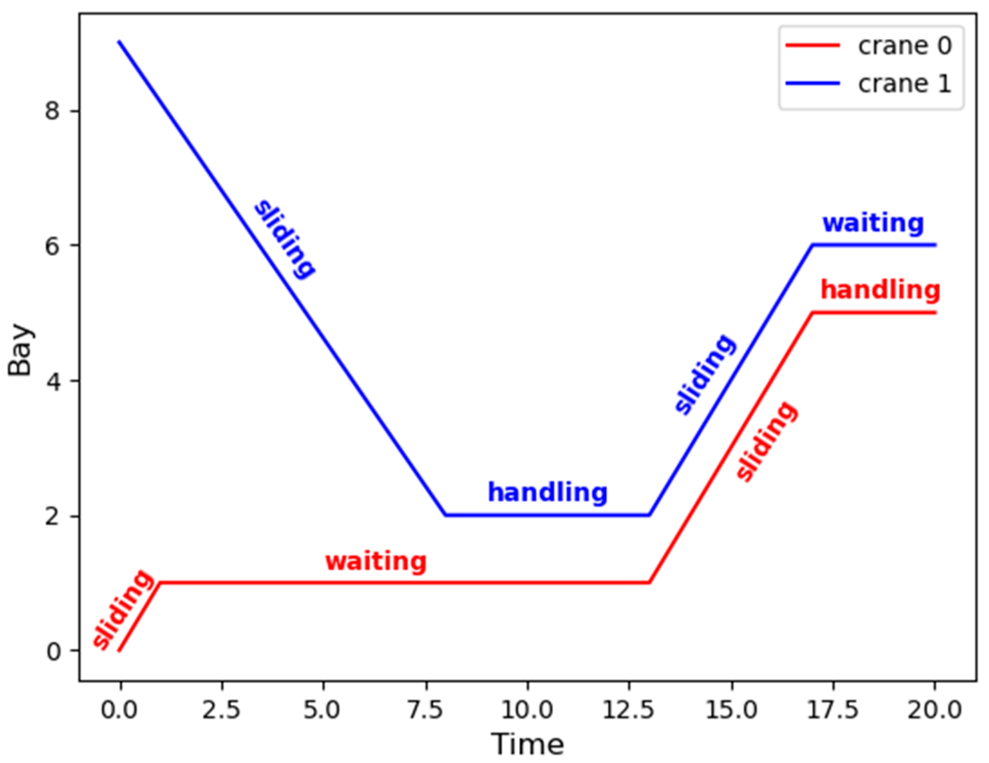
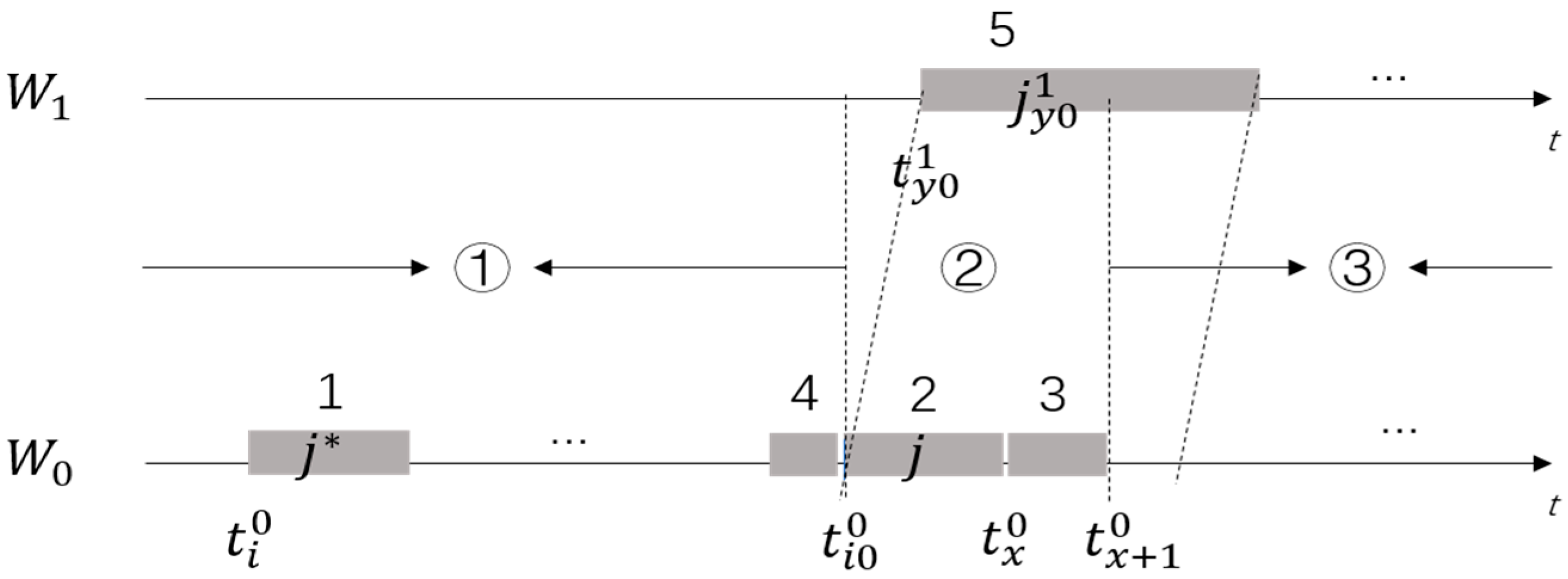
Assume that the task release time of task I of yard crane 0 changes, as shown in Figure 2, which is a time-domain diagram of local re-scheduling strategy. In Figure 2, “W₀” and “W₁” represent the initial scheduling timelines of cranes 0 and 1, respectively. Labels 1 to 5 are the specific time periods on the timeline “W₀” and “W₁” that need to be partially rescheduled. The gray part on the timeline represents the time occupancy of the corresponding task.

Label 1 corresponds to the original handling period of task i, and $t_i^0$ represents the original $j_i^0:ST$ on the timeline. Label 2 corresponds to the new handling period of task i after rescheduling, which meets the constraint of release time. Label $t_{i0}^0$ indicates the time when task i needs to be re-inserted. After the insertion, the new number for task i is i₀. Then, the time period 1 would become a no-handling period of crane 0 to avoid increasing interference (crane 0 waits after reaching the destination position while the spreader does not move).

The time period of label 3 ensures that yard crane 0 returns to the target location of task $j_{i0-1}^0$ when the newly inserted task is handled. During $t_{x }^0$ ~ $t_{x+1}^0$, yard crane 0 will move to the target location of task $j_{i0-1}^0$.

After the local re-scheduling of labels 1 to 3 is completed, add detour task to yard crane 0 if there is interference at label 3. Additionally, there will be a local re-scheduling task at label 4, in which the yard crane 0 gives way to yard crane 1 until yard crane 1 completes the current task. In this way, there are no other changes for yard crane 0 except that the locations of labels 2, 3, and 4 are changed. It makes the non-crossing constraints between the yard cranes satisfied in the time period at the time period marked ① in Figure 2.

Label 5 corresponds to the detour task of yard crane 1. Finally, yard crane 1 will return to the initial location, that is, the starting location of task $j_{y0}^1$. The detour task time is determined by the extension time of yard crane 0. It keeps yard crane free of interference at the time periods of labels ② and ③. By means of above steps, a new scheduling is obtained based on the original optimal scheduling.

As mentioned above, the algorithm starts from a static initial optimal scheduling. It is assumed that the release time of crane 0 task i is delayed, $j_i^0:Rd\to j_i^0:R{d}^{*}$. The steps of the algorithm are described in Algorithm 2:

Algorithm 2: The Algorithm Steps

Step 1. Find the insertion point i0. Take the minimum value of i0, $i_0\in \left\{i_0=e-1\right\}\cup min\{j_{i0}^0:Rd>0\cap j_i^0:R{d}^{*}\ge j_{i0}^0:ST\}$. If $i_0\le i$, turn to step 5; otherwise, turn to the next step. Step 2. Insert task i ($i\in \{j_i^0:Job=j\}$) into position of task i0 in the task list. Revalue $j_{e-1}^0:Rd=j_i^0:R{d}^{*}$,$j_i^0:Job=$−3. If $i_0=e-1$, turn to step 4; otherwise, turn to the next step. Step 3. As label “$j_{x-1}^0$” and label “$j_{i0-1}^0$” are shown in Figure 2, if $j_{x-1}^0:Bay\ne j_{i0-1}^0:Bay$, insert a task $j_x^0$ into task x in the task list, set $j_x^0:Bay=j_{i0-1}^0:Bay$, $j_x^0:Row=j_{i0-1}^0:Row$, $j_x^0:Job=-4$, and set the remaining parameters to zero. If $j_{x-1}^0:Bay=j_{i0-1}^0:Bay$, turn to the next step. Step 4. As label “y0” shown is in Figure 2, get the value of y0, $y_0\in \left\{y_0=e-1\right\}\cup min\left\{j_{y0}^1: ST\ge j_{i0}^0 \right\}$. When there is interference between crane 0′s whole tasks and crane 1′s tasks 0 to $j_{y0-1}^1$, crane 0 makes way. Crane 1 gives way to the bay 9 of the yard, and returns to the initial position $j_{y0-1}^1:Bay$ at the end of the detour. The time it takes for crane 1 to give way is equal to the delay of crane 0. Then, insert the detour task for crane 1 into task y0 in the task list of crane 1. Step 5. Update the release time of task i, $j_i^0:Rd=j_i^0:R{d}^{*}$. Step 6. End.

5. Computational Experiments

5.1. Parameter Setting

The size of each yard is set to bay ∈ [0, 9], row ∈ [0, 5] (the yard data refer to the parameters of Qingdao Xinqianwan automated terminal). Yard crane ∈ {0,1}. The particle swarm size is set to 10, the weight is 0.729, the cognitive coefficient and the social coefficient are 1.494, and the number of iterations is 50.

It adopts MacBook Pro 13 (from Apple, Cupertino, CA, USA) with 2.3 GHz quad-core Intel Core i5 processor, 8 GB 2133 MHz LPDDR3 memory, and the programming language is Python 3.8 (from Python Software Foundation, Wilmington, DE, USA).

5.2. The Effectiveness Experiments

Randomly generate a task group with 20 tasks, as shown in

Table 5. Initial tasks.

Task	Bay	Row	Time	Release Time
1	1	2	4	0
2	5	3	4	0
3	6	1	4	0
4	1	3	4	0
5	4	4	2	0
6	5	2	4	0
7	2	1	4	0
8	7	2	1	0
9	8	3	4	0
10	7	4	3	0
11	8	1	6	0
12	1	2	4	0
13	6	3	4	0
14	2	3	3	0
15	6	4	2	0
16	4	3	4	0
17	5	2	4	0
18	7	1	4	0
19	2	4	1	0
20	8	4	2	0

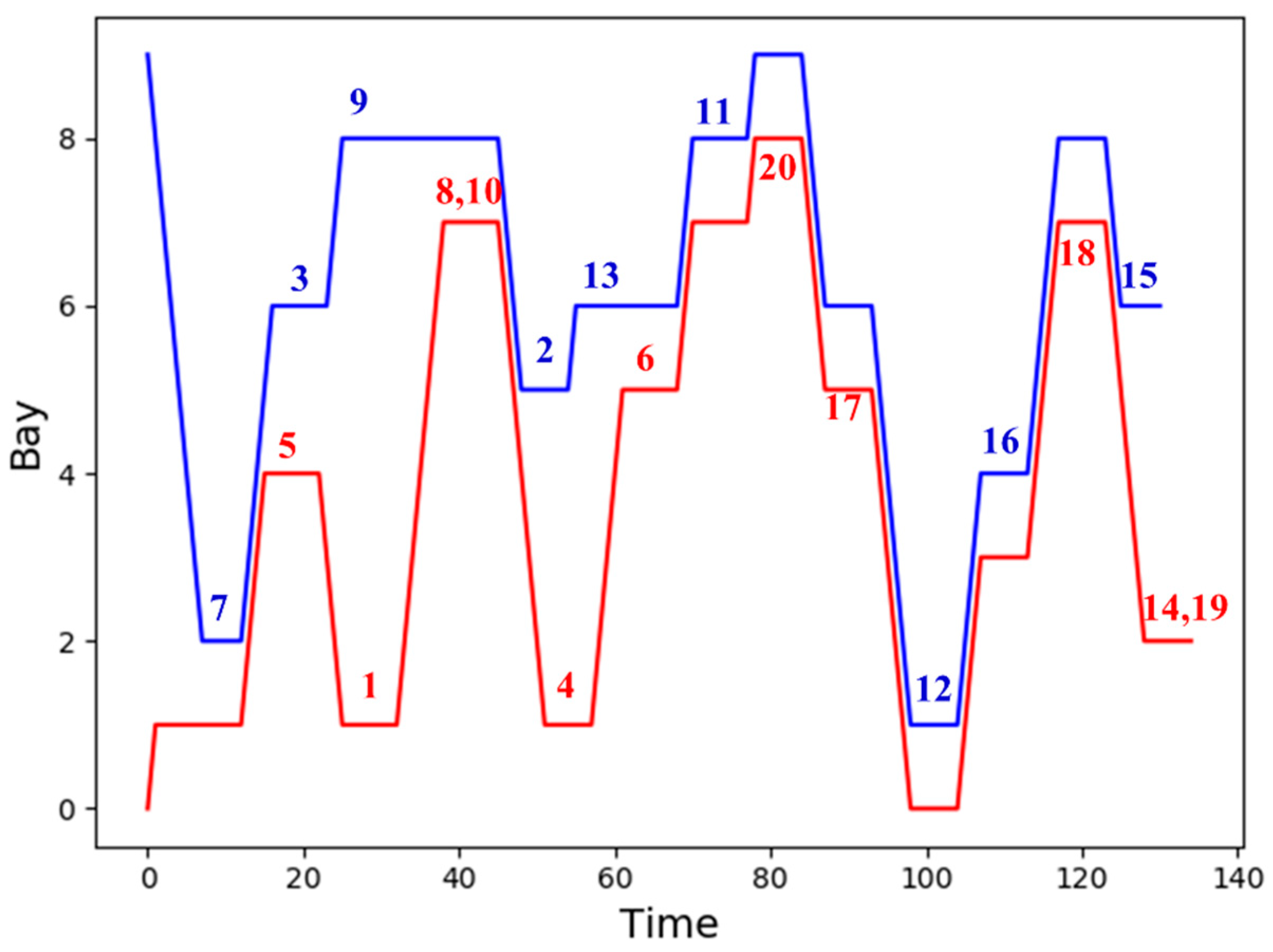
. In the table, the representations of “Task”, “Bay”, “Row”, “Time”, and “Release Time” are the same as those in Section 3.1. The particle swarm algorithm is used to find the initial global solution. Firstly, the algorithm generates scheduling particles according to the task information provided in Table 5. The scheduling particles include the task allocation of yard cranes 0 and 1, the scheduling sequence, and the priority of each yard crane task. Then, the particle swarm algorithm is used to obtain an optimal or near-optimal solution. The best result obtained by PSO is shown in Figure 3. Figure 3 gives a spatiotemporal diagram of yard cranes 0 (red line) and 1 (blue line). The horizontal axis represents the time, and the vertical axis represents the bay location of the yard crane. All tasks’ numbers are displayed in the figure according to their handling time and bay locations. The red/blue number indicates that the task was handled by crane 0/1. It can be seen that there is no collision between yard cranes 0 and 1; that is, the algorithm can obtain a solution that meets the constraints.

Table 6. Tasks’ release time renewal.

Number	Bay	Row	Time	Release Time
1	1	2	4	27
2	5	3	4	17
3	6	1	4	35
4	1	3	4	11
5	4	4	2	48
6	5	2	4	20
7	2	1	4	55
8	7	2	1	14
9	8	3	4	28
10	7	4	3	14
11	8	1	6	30
12	1	2	4	43
13	6	3	4	10
14	2	3	3	23
15	6	4	2	19
16	4	3	4	61
17	5	2	4	48
18	7	1	4	19
19	2	4	1	13
20	8	4	2	32

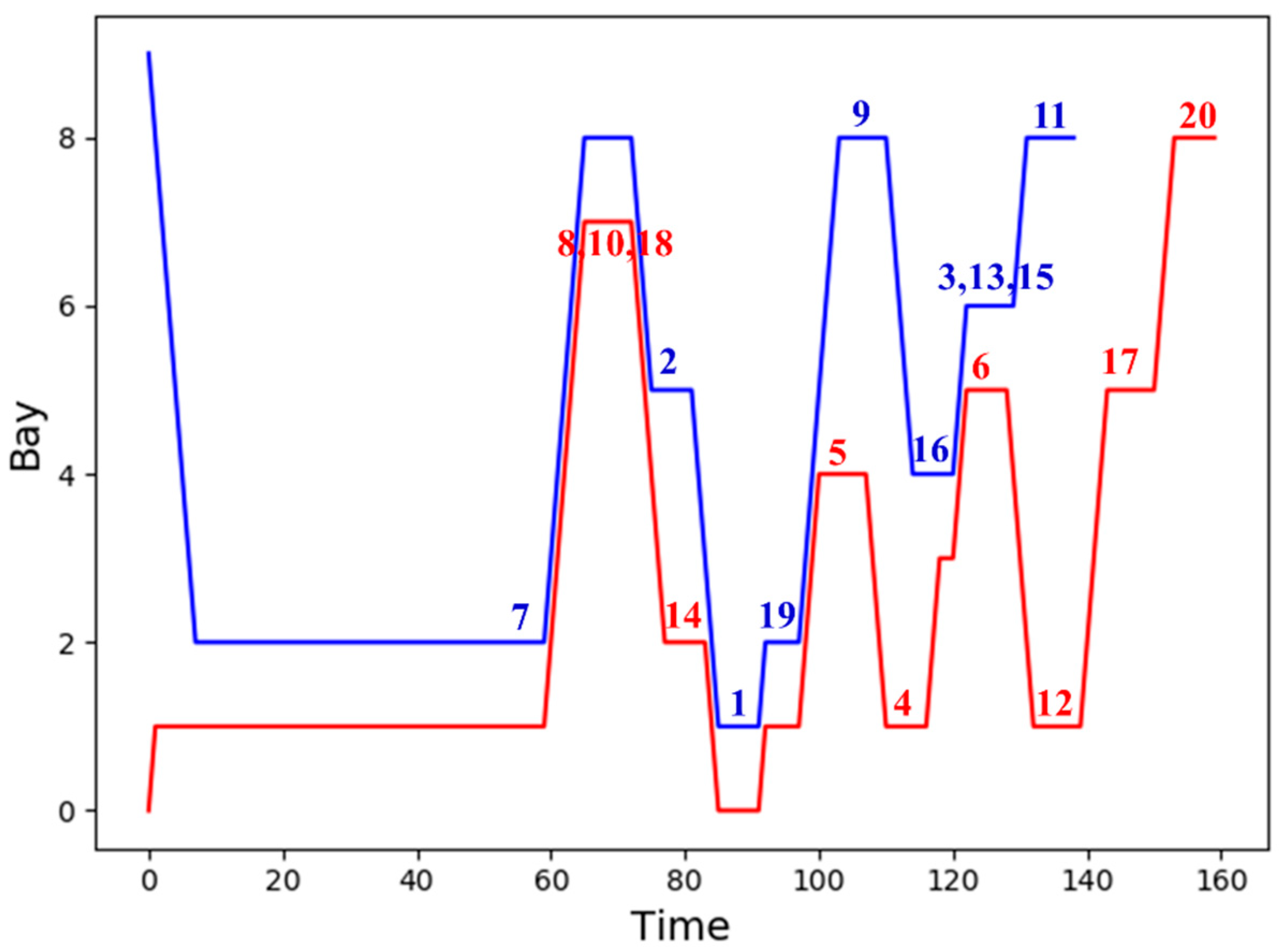
shows the changes in the “Release Time” of Table 5. Figure 4 shows the results obtained by LRPSO in Table 6. Same as Figure 3, the task numbers are displayed in the figure. From Figure 4, it can be seen that all tasks are handled after their release time, and the overall completion time becomes longer after the task release time changes. The yard cranes complete all tasks without collisions, so LRPSO meets the constraints.

It can be seen that the joint scheduling method including PSO and local re-scheduling is effective.

5.3. Simulation Comparison

Simulation experiments are carried out for different task scales and different task release time ranges (variation ranges). The compared algorithms are global strategy algorithm and PSO algorithm. After the release time of tasks changed, the global strategy algorithm always re-solves the fitness value (completion time) according to the original optimal plan. The PSO algorithm re-solves iteratively according to the new tasks.

In each set of simulation experiments, the PSO algorithm is first used to generate an initial optimal planning solution. Then, the release time of some tasks in the original task group are randomly changed according to the variation range, and three algorithms are used to solve the dynamic task group. Finally, the performance of the algorithms is compared in terms of calculation time and fitness value results.

Comparison results are given in

Table 7. Simulation comparison data.

N	Variation Range	CPU Time (s)			Completion Time
		LRPSO	Global Strategy	PSO	LRPSO	Global Strategy	PSO
500	5%	0.5	2.1	626.3	5058	5983	5021
	15%	0.2	2.5	646.2	5682	6389	5613
	25%	0.8	2.3	651.3	5467	6526	5481
	50%	1.1	2.6	677.5	7907	6596	6234
	75%	1.4	2.3	689.3	6533	6549	6399
1000	5%	1.1	4.4	1292.4	8795	13,318	11,731
	15%	1.5	4.7	1260.3	9895	13,052	12,249
	25%	1.6	4.9	830.9	10,770	12,972	12,373
	50%	2.1	4.3	840.9	13,843	13,299	12,602
	75%	2.9	4.2	858.3	16,050	13,170	12,869
1500	5%	1.6	6.4	1366.4	8651	13,120	11,413
	15%	1.8	6.5	1163.5	9288	11,482	11,230
	25%	2.1	6.5	1345.7	10,105	11,515	11,586
	50%	2.8	6.6	1325.5	12,133	12,113	11,820
	75%	3.7	6.5	1344.1	14,194	12,149	11,884
2000	5%	2.2	8.7	1833.5	11,339	14,962	14,164
	15%	2.8	9.1	1766.6	12,167	15,253	14,954
	25%	3.4	8.8	1759.5	15,841	22,105	21,564
	50%	5.4	9.0	1736.3	18,800	18,217	18,243
	75%	8	9.0	1985.5	23,309	18,537	18,303

, where “N” represents the total number of tasks; “variation range” refers to the variation range of the overall tasks’ release time, “0” means that there is no change, and “100%” means that all the tasks’ release time are changed. “CPU Time” represents the calculation time of algorithms in seconds, and the recorded results are kept to one decimal place.

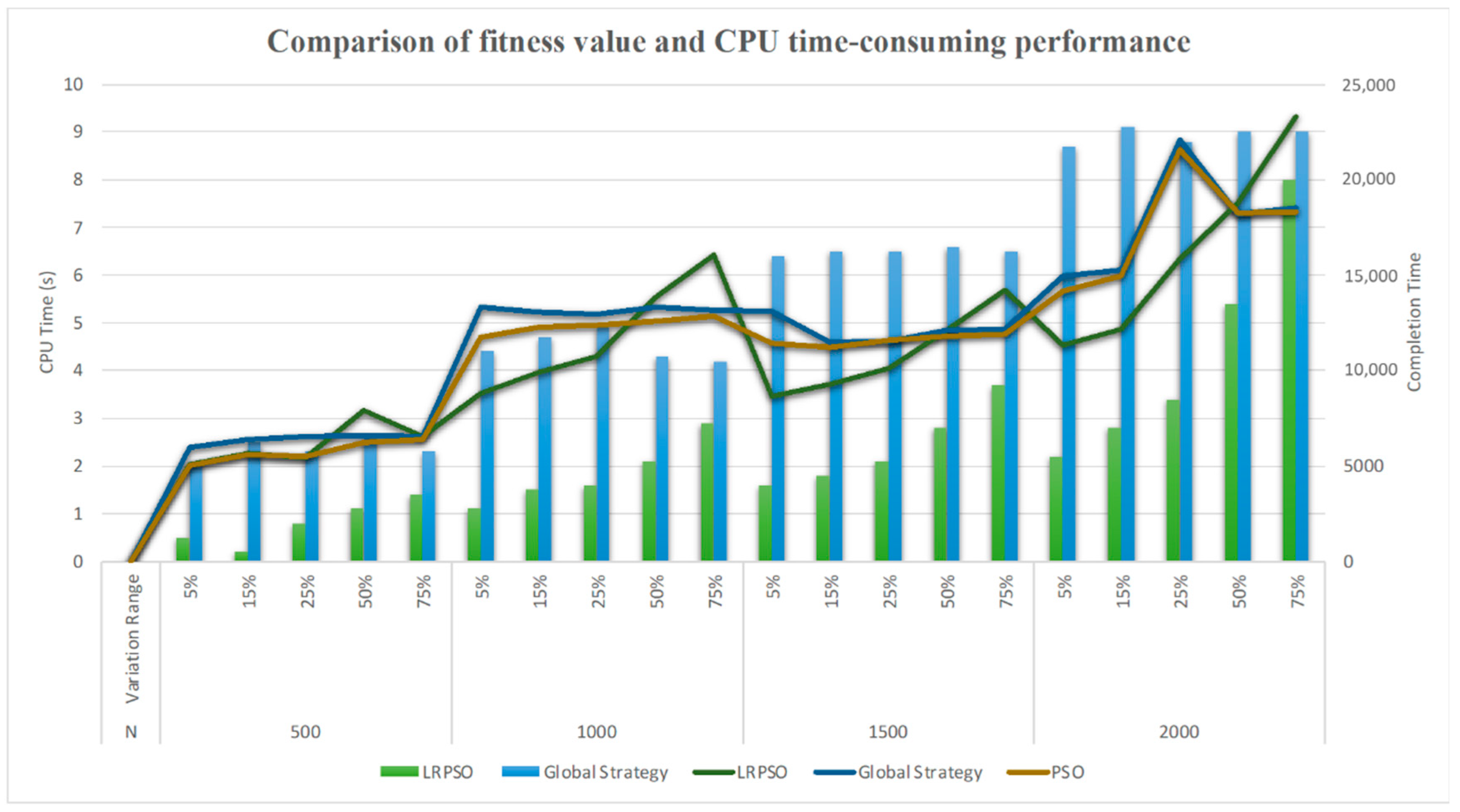
Figure 5 summarizes the CPU time and the solution results of LRPSO, global strategy algorithm, and PSO algorithm under different task scales based on the data in Table 7. The histogram shows the CPU time, and the line graph shows the fitness values. Since the CPU time of PSO far exceeds that of the other two algorithms, it is not shown. On the whole, as the task scale increases, the solution time of each algorithm increases. The CPU time of the LRPSO is much shorter than other two algorithms. When the release time variation range is less than 50%, the solutions of the LRPSO are better than other algorithms. Under the same task scale, the solution time of the LRPSO increases with the increase of the task variation range. As the task scale increases, the trend of time spent and solution results shows obvious regularity: when the release time variation range exceeds 50%, the increase rate of the solution time and fitness value solution results is accelerated, and the slope becomes steeper. It can be seen that the performance of the LRPSO is better than other algorithms within the release time variation range of 50%. When the release time variation range exceeds 50%, the performance of the LRPSO is greatly reduced compared with other algorithms and is no longer applicable.

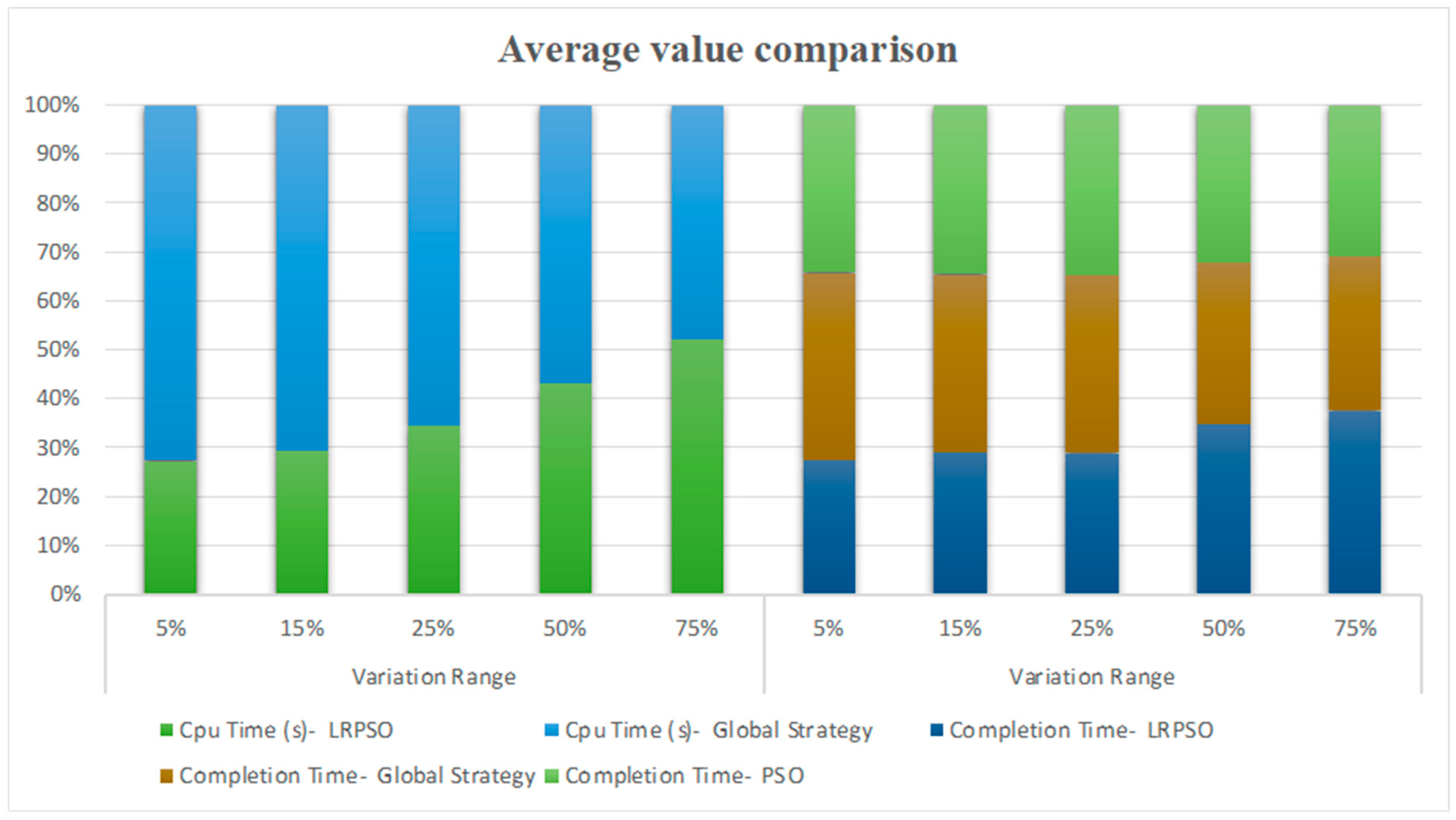
Figure 6 shows the average CPU time and average solutions of each algorithm under different release time variation ranges. In the figure, the left half shows the CPU time comparison, and the right half shows the completion time comparison. The same is shown with Figure 5: since the average CPU time of PSO far exceeds that of the other two algorithms, it is not shown. It can be seen that when the release time variation range does not exceed 50%, the LRPSO has a better performance.

From the comparison results, it can be seen that the LRPSO can be applied to large-scale dynamic yard crane scheduling with a release time variation range less than 50%.

6. Conclusions

Aiming at improving the flexibility of the terminal yard, this paper studies the twin yard cranes scheduling problem, considering the dynamic cut-off time and no-crossing constraint. The dynamic cut-off time makes the release time of the yard crane variable, and the yard crane task arrangement will change frequently, resulting in a lot of computing time. To decrease the computing time and improve the terminal yard efficiency, a joint scheduling strategy of PSO and local re-scheduling is proposed. This solution method is proved to be effective and practical, and it is easier to be optimized and extended. The contributions of this paper are as follows: (1) a twin yard cranes scheduling model is built considering environment variables, which is closer to reality; (2) a local re-scheduling strategy joint with PSO is proposed, which can improve the adaptability of yard crane scheduling to environmental variables and other influencing factors. The experiment results show that LRPSO has better performance compared with the global strategy and PSO in the large-scale scheduling with the release time variable variation range less than 50%.

We will use more scheduling methods for comparison in future research, such as polynomial-time, heuristics, genetic algorithms, and so on. Another further study is to set both task release time and task processing time as dynamic variables. Furthermore, we will also concentrate on optimizing the schedule of the initial retrieval and storage of yard cranes, taking container storage scheduling of the yard into consideration, and optimizing the cooperation of automated guided vehicles and yard cranes.