
Corrosion Prediction Models in the Reinforcement of Concrete Structures of Offshore Wind Farms


Abstract
:1. Introduction
2. Materials and Methods
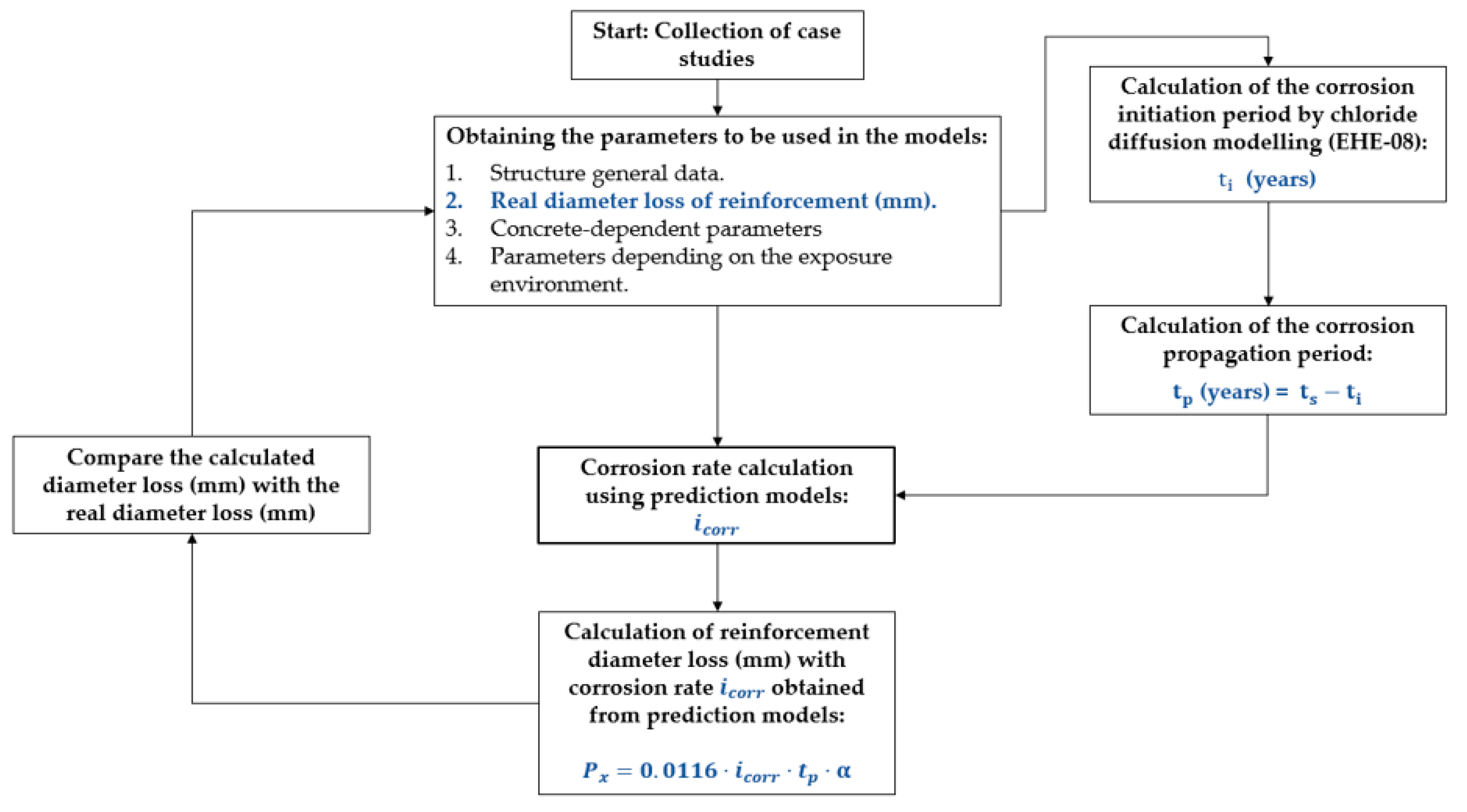
2.1. General Methodology
2.2. Systematic Analysis of Corrosion Prediction Models
2.2.1. Chloride Diffusion Model
2.2.2. Corrosion Rate Calculation Models
Liu and Weyers (1998)
Vu and Stewart (2000)
Li (2004 a)
Li (2004 b)
Kong et al. (2006)
New Empirical Model (Lu et al., 2019)
3. Case Study Description
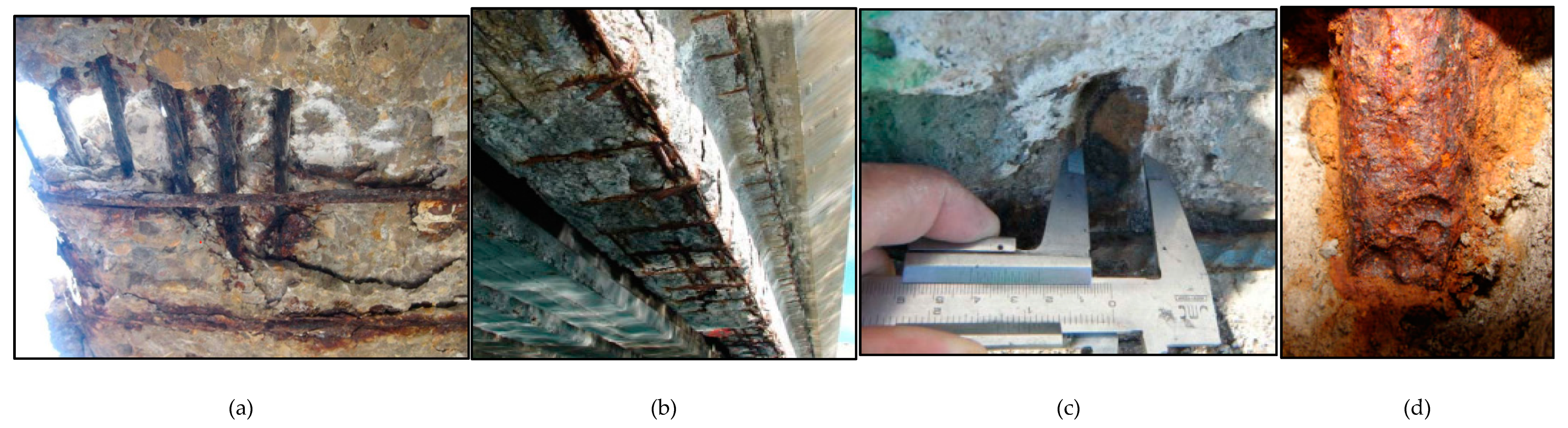
3.1. Selection of Case Studies
- Concrete-dependent: chloride concentration at reinforcement position, w/c ratio, concrete cover, and compressive strength of concrete.
- Exposure environment of the structure: temperature and relative humidity.
3.2. Model Parameters
3.2.1. Concrete-Dependent Parameters
- Porosities between 12–14%, a w/c ratio of 0.45 to 0.50 is established.
- Porosities between 14–16%, a w/c ratio of 0.55 to 0.60 is established, although the latter value (0.60) can lead to even somewhat higher porosity values.
3.2.2. Parameters Depending on the Exposure Environment
4. Results
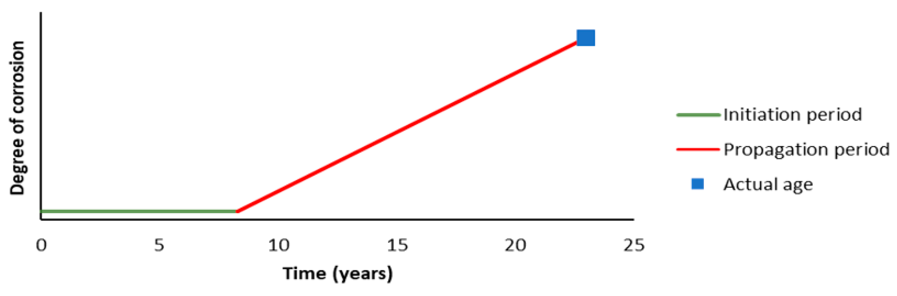
4.1. Propagation Period
4.2. Calculation of Diameter Loss
4.2.1. Liu & Weyers (1998)
4.2.2. Vu and Stewart (2000)
4.2.3. Li (2004 a)
4.2.4. Li (2004 b)
4.2.5. Kong et al. (2006)
4.2.6. New Empirical Model (Lu et al., 2019)
5. Discussion
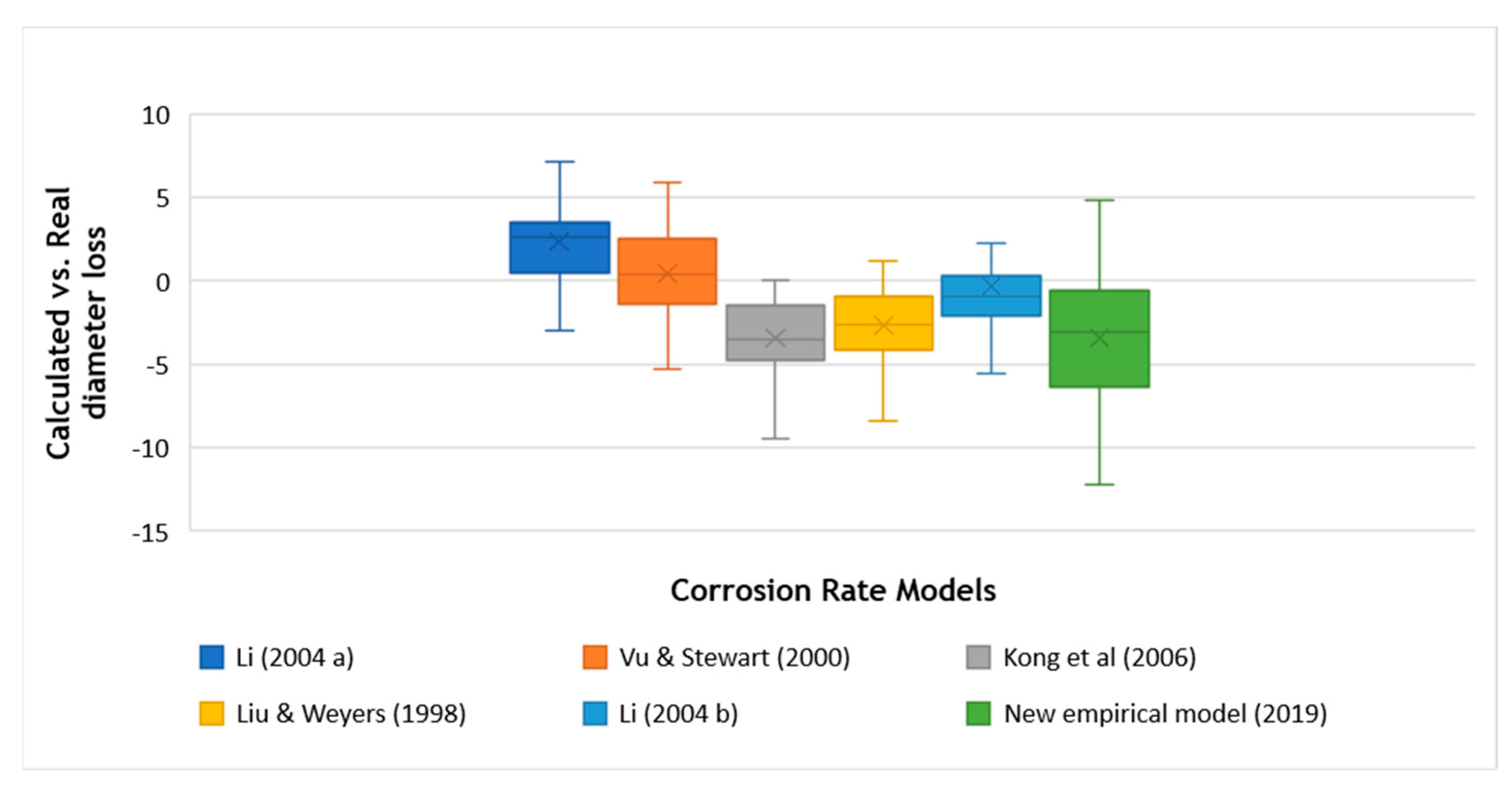
5.1. Comparison of Model Results
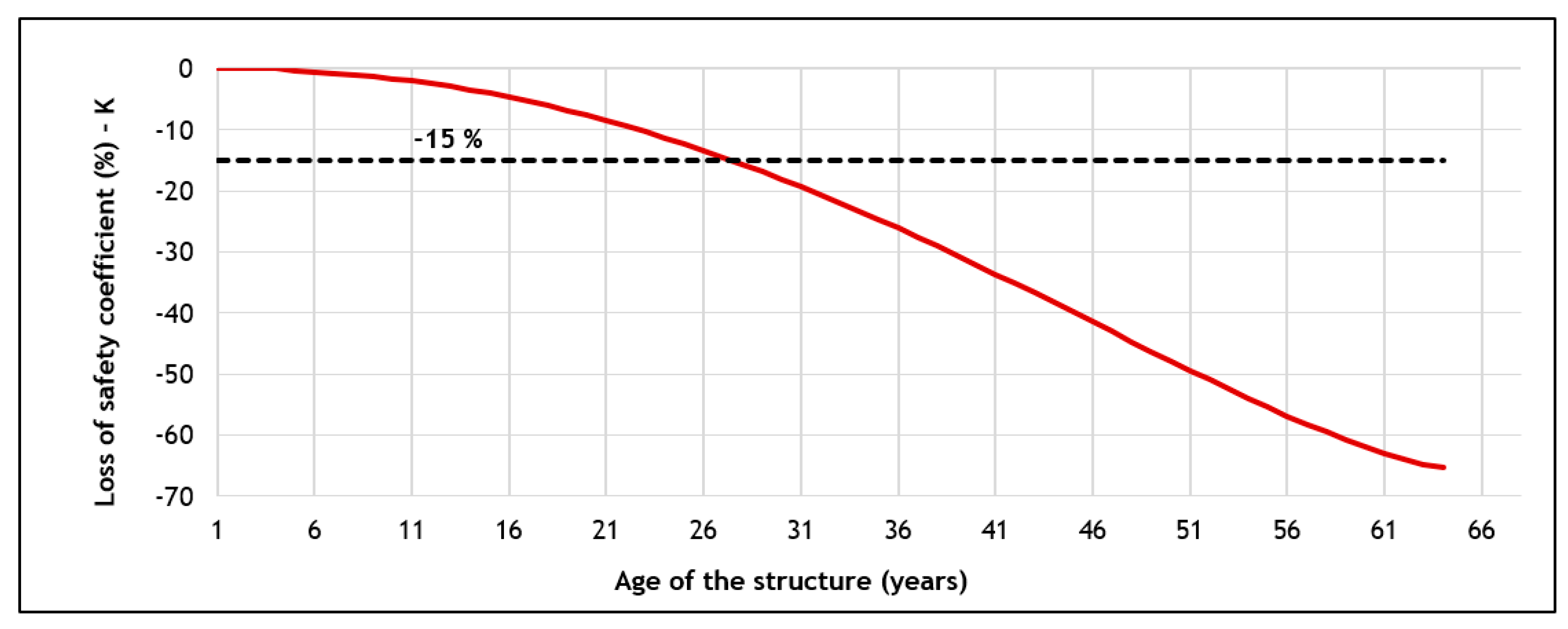
5.2. Potential Applications
6. Conclusions
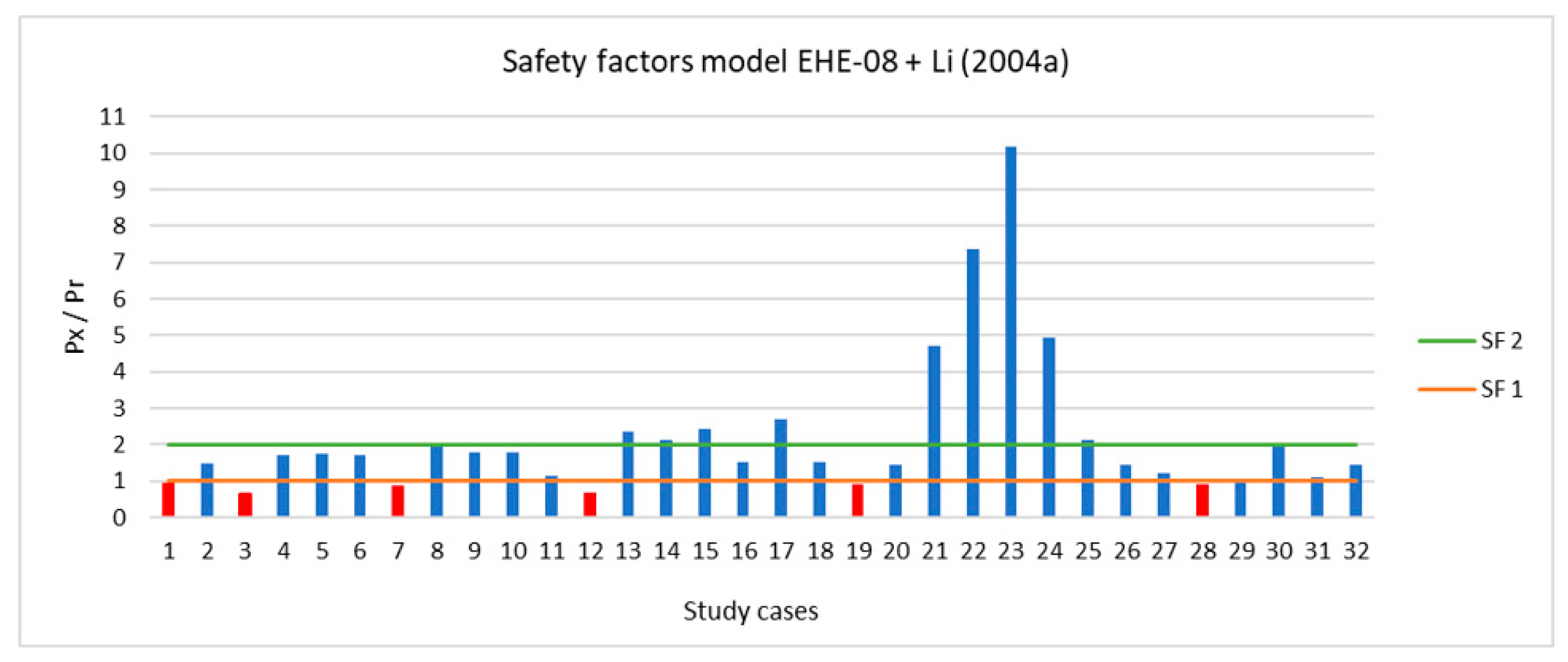
- In more than 75% of the 32 case studies, the application of the chloride diffusion model of the EHE-08 and the corrosion rate calculation model of Li (2004 a) has resulted in similar diameter loss values when compared to real reinforced and prestressed concrete structures that have been affected by active corrosion processes. The calculated diameter loss results promise reasonable safety coefficients, with a minimum value of 1.73, and the average safety factor of 1.98. This means that the diameter loss value calculated through the models is twice as high as the actual diameter loss.
- The combination of the EHE-08 diffusion model and the Vu and Stewart (2000) corrosion rate calculation model is the next best performer in diameter loss. In this case, the median is zero, which means that the combination of models has approximately the same probability of success as failure in a case study.
- The combination of the EHE-08 chloride diffusion model and the other corrosion rate calculation models: Liu and Weyers (1998), Li (2004 b), Kong et al. (2006), and New Empirical Model (Lu et al., 2019) has not obtained satisfactory results. The calculated reinforcement diameter losses were generally much lower in practically all cases, with the combination with the model of Kong et al. (2006) giving the worst results.
- The application of the EHE-08 diffusion model with none of the corrosion rate calculation models proposed, has proved satisfactory results in the case studies of prestressed and post-tensioned concrete structures analyzed as part of the whole sample. Again, the model of Li (2004 a), together with the chloride diffusion model of the EHE-08, gave the best results in this aspect.
- A tool for rapidly estimating the section loss of reinforcement in offshore concrete structural elements as a function of time provides offshore wind farm operators with a cost-effective approach for planning their maintenance strategies and the optimisation of material costs and human resources. This is essential, considering the exponential expansion of OWF’s, which will only be compatible if this type of proposal contributes to the reduction of O&M costs, and where reinforced concrete will continue to be represented.
Author Contributions
Funding
Institutional Review Board Statement
Informed Consent Statement
Data Availability Statement
Acknowledgments
Conflicts of Interest
References
- Ramírez, L.; Brindley, G. Offshore Wind Energy: 2021 Mid-Year Statistics. 2021. Available online: Windeurope.org (accessed on 10 November 2021).
- Lee, J.; Zhao, F. Global Offshore Wind Report 2021. 2021. Available online: http://www.gwec.net/global-figures/wind-energy-global-status/ (accessed on 10 November 2021).
- International Renewable Energy Agency. Renewable Energy Statistics 2021. 2021. Available online: https://www.irena.org/publications/2021/March/Renewable-Capacity-Statistics-2021 (accessed on 10 November 2021).
- European Union. Regulation (EU) 2021/1119 of the European Parliament and of the Council of 30 June 2021 Establishing the Framework for Achieving Climate Neutrality and Amending Regulations (EC) No 401/2009 and (EU) 2018/1999 (‘European Climate Law’). 2021. Available online: https://eur-lex.europa.eu/legal-content/EN/TXT/PDF/?uri=CELEX:52019DC0640&from=EN (accessed on 10 November 2021).
- European Commission. In-Depth Analysis in Support of the Commission Communication Com (2018) 773: A Clean Planet for all A European Long-Term Strategic Vision for a Prosperous, Modern, Competitive and Table of Contents. 2018. Available online: https://knowledge4policy.ec.europa.eu/publication/depth-analysis-support-com2018-773-clean-planet-all-european-strategic-long-term-vision_en (accessed on 10 November 2021).
- European Commission. Guidance Document on Wind Energy Developments and EU Nature Legislation. 2020. Available online: https://ec.europa.eu/environment/nature/natura2000/management/docs/wind_farms_en.pdf (accessed on 15 October 2021).
- Fraile, I.K.D.; Vandenberghe, A.; Klonari, V.; Ramirez, L.; Pineda, I.; Tardieu, P.; Malvault, B. Getting Fit for 55 and Set for 2050. 2021. Available online: https://windeurope.org/intelligence-platform/product/getting-fit-for-55-and-set-for-2050/# (accessed on 10 November 2021).
- Johnston, B.; Foley, A.; Doran, J.; Littler, T. Levelised cost of energy, A challenge for offshore wind. Renew. Energy 2020, 160, 876–885. [Google Scholar] [CrossRef]
- Mone, C.; Stehly, T.; Maples, B.; Settle, E. 2017 Cost of Wind Energy Review. 2017. Available online: https://www.nrel.gov/docs/fy18osti/72167.pdf (accessed on 15 March 2021).
- Crabtree, C.J.; Zappalá, D.; Hogg, S.I. Wind energy: UK experiences and offshore operational challenges. Proc. Inst. Mech. Eng. Part A J. Power Energy 2015, 229, 727–746. [Google Scholar] [CrossRef] [Green Version]
- BVG. Associates. Value Breakdown for The Offshore Wind Sector. 2010. Available online: https://www.gov.uk/government/uploads/system/uploads/attachment_data/file/48171/2806-value-breakdown-offshore-wind-sector.pdf (accessed on 12 April 2021).
- Miedema, R. Offshore Wind Energy Operations & Maintenance Analysis. Research Thesis, Hogeschool Van Amsterdam, Amsterdam, The Netherlands. 2012. Available online: http://sciencecentre.amccentre.nl/studies/Thesis_Robert_Miedema.pdf (accessed on 15 March 2021).
- Wu, X.; Hu, Y.; Li, Y.; Yang, J.; Duan, L.; Wang, T.; Adcock, T.; Jiang, Z.; Gao, Z.; Lin, Z.; et al. Foundations of offshore wind turbines: A review. Renew. Sustain. Energy Rev. 2018, 104, 379–393. [Google Scholar] [CrossRef] [Green Version]
- Sánchez, S.; López-Gutiérrez, J.S.; Negro, V.; Esteban, M.D. Foundations in offshore wind farms: Evolution, characteristics and range of use. Analysis of main dimensional parameters in monopile foundations. J. Mar. Sci. Eng. 2019, 7, 441. [Google Scholar] [CrossRef] [Green Version]
- Esteban, M.D.; Matutano, C. Offshore Wind Foundation Design: Some Key Issues. J. Energy Resour. Technol. 2015, 137, 1–6. [Google Scholar] [CrossRef]
- Fernández, R.P.; Pardob, M.L. Offshore concrete structures. Ocean Eng. 2013, 58, 304–316. [Google Scholar] [CrossRef]
- Esteban, M.D.; López-Gutierrez, J.-S.; Negro, V. Gravity-Based Foundations in the Offshore Wind Sector. J. Mar. Sci. Eng. 2019, 7, 64. [Google Scholar] [CrossRef] [Green Version]
- Trust, T.C. Offshore Wind Industry Review of GBS. 2015. Available online: https://prod-drupal-files.storage.googleapis.com/documents/resource/public/Offshore_wind_industry_review_of_Gravity_Based_Structures_REPORT.pdf (accessed on 20 December 2021).
- Esteban, M.D.; Couñago, B.; López-gutiérrez, J.S.; Negro, V.; Vellisco, F. Gravity based support structures for offshore wind turbine generators: Review of the installation process. Ocean Eng. 2015, 110, 281–291. [Google Scholar] [CrossRef]
- Rodrigues, S.; Restrepo, C.; Kontos, E.; Pinto, R.T.; Bauer, P. Trends of offshore wind projects. Renew. Sustain. Energy Rev. 2015, 49, 1114–1135. [Google Scholar] [CrossRef]
- WindEurope—The Voice of the Wind Energy Industry. Available online: https://windeurope.org/ (accessed on 16 December 2021).
- Mathern, A.; von der Haar, C.; Marx, S. Concrete support structures for offshore wind turbines: Current status, challenges, and future trends. Energies 2021, 14, 1995. [Google Scholar] [CrossRef]
- ELISA—Elican Project. Esteyco. Available online: https://www.esteyco.com/proyectos/elisa-elican-project/ (accessed on 16 December 2021).
- James, R.; Ros, M.C. Floating Offshore Wind: Market and Technology Review. Carbon Trust 2015, 439. [Google Scholar] [CrossRef]
- International Renewable Energy Agency (IRENA). Innovation Outlook: Offshore Wind. Available online: https://www.irena.org/publications/2016/oct/innovation-outlook-offshore-wind (accessed on 12 December 2021).
- DNV GL. DNVGL-ST-0126: Support Structures for Wind Turbines. 2018. Available online: https://rules.dnvgl.com/docs/pdf/DNVGL/ST/2018-07/DNVGL-ST-0126.pdf (accessed on 15 May 2021).
- ACI Committee 222. Protection of Metals in Concrete Against Corrosion. In Aci 222R-01; ACI: Farmington Hills, MI, USA, 2001; pp. 1–41. [Google Scholar]
- EC Innovation Programme; Andrade, C.; Izquierdo, D. A Validated Users Manual for Assessing the Residual Service Life of Concrete Structures. Madrid. 2001. Available online: https://www.ietcc.csic.es/wp-content/uploads/1989/02/manual_contecvet_ingles.pdf (accessed on 20 October 2021).
- Feliu, S.; Andrade, C. Manual: Inspección de Obras Dañadas por Corrosión de Armaduras. In Acor; IETCC: Madrid, Spain, 1989; pp. 1–122. [Google Scholar] [CrossRef]
- Odriozola, M.Á.B. Corrosión de las Armaduras del Hormigón Armado en Ambiente Marino: Zona de Carrera de Mareas y Zona Sumergida. Ph.D. Thesis, Universidad Politécnica de Madrid, Madrid, Spain, 2007. [Google Scholar]
- Pruckner, F. Diagnosis and Protection of Corroding Steel in Concrete. Ph.D. Thesis, Norwegian University of Science and Technology Faculty of Engineering Science and Technology Department of Structural Engineering, Trondheim, Norway, November 2002. [Google Scholar]
- Ciolko, A. Nondestructive Methods for Condition Evaluation of Prestressing Steel Strands Nondestructive Methods for Condition Evaluation of Prestressing Steel Strands in Concrete Bridges Final Report Phase I: Technology Review; Prepared for National Cooperative Highway Research Program; no. July 2015; NCHRP: Washington, DC, USA, 1999.
- Liu, L.; Fu, Y.; Ma, S.; Huang, L.; Wei, S.; Pang, L. Optimal scheduling strategy of O&M task for OWF. IET Renew. Power Gener. 2019, 13, 2580–2586. [Google Scholar] [CrossRef]
- Shafiee, M. Maintenance logistics organization for offshore wind energy: Current progress and future perspectives. Renew. Energy 2015, 77, 182–193. [Google Scholar] [CrossRef]
- Lu, Z.H.; Lun, P.Y.; Li, W.; Luo, Z.; Li, Y.; Liu, P. Empirical model of corrosion rate for steel reinforced concrete structures in chloride-laden environments. Adv. Struct. Eng. 2019, 22, 223–239. [Google Scholar] [CrossRef]
- Tutti, K. Corrosion of Steel in Concrete. Swedish Cement and Concrete Research Institute. 1982. Available online: http://www.cbi.se/viewNavMenu.do?menuID=317&oid=857 (accessed on 15 May 2021).
- García, S.F. Corrosión De Armaduras En El Hormigón Armado En Ambiente Marino Aéreo. Ph.D. Thesis, Universidad Poltécnica de Madrid, Madrid, Spain, 2016. Available online: https://oa.upm.es/39374/1/Susana_Fernandez_Garcia.pdf (accessed on 16 April 2021).
- Comisión Permanente del Hormigón. Instrucción de Hormigón Estructural (EHE-2008). 2011. Available online: http://www.ponderosa.es/docs/Norma-EHE-08.pdf (accessed on 20 December 2021).
- Helland, S.; Aarstein, R.; Maage, M. In-field performance of North Sea offshore platforms with regard to chloride resistance. Struct. Concr. 2010, 11, 15–24. [Google Scholar] [CrossRef]
- Markeset, G.; Mytdal, R. Modelling of Reinforcement Corrosion in Concrete-State of the Art. 2008. Available online: http://smartpipe.com/upload/Byggforsk/Publikasjoner/coin-no7.pdf (accessed on 22 February 2021).
- Bertolini, L.; Elsener, B.; Pedeferri, P.; Redalli, E.; Polder, R. Corrosion of Steel in Concrete. Prevention, Diagnosis, Repair; Wiley: Hoboken, NJ, USA, 2013. [Google Scholar]
- Zhang, D.; Zeng, Y.; Fang, M.; Jin, W. Service life prediction of precast concrete structures exposed to chloride environment. Adv. Civ. Eng. 2019, 2019, 3216328. [Google Scholar] [CrossRef]
- Liu, Y. Modeling time-to-corrosion cracking in chloride contaminated reinforced concrete structures. ACI Mater. J. 1999, 96, 611–613. Available online: https://trid.trb.org/view/514367 (accessed on 15 April 2021).
- Yu, B.; Yang, L.; Wu, M.; Li, B. Practical model for predicting corrosion rate of steel reinforcement in concrete structures. Constr. Build. Mater. 2014, 54, 385–401. [Google Scholar] [CrossRef]
- Gjørv, O.E. Durability Design of Concrete Structures in Severe Environments; Routledge: Abingdon-on-Thames, UK, 2014. [Google Scholar]
- Ministerio de Obras Públicas. Instrucción para el Proyecto y la Ejecución de Obras de Hormigón en Masa o Armado (EH-88); Ministerio de Obras Públicas: Madrid, Spain, 1988.
- Ministerio de Obras Públicas. Instrucción para el Proyecto y Ejecución de Obras de Hormigón, 1st ed.; Ministerio de Obras Públicas: Santander, Spain, 1939; Volume 1.
- Agencia Estatal de Meteorología—AEMET. Gobierno de España. Available online: http://www.aemet.es/es/portada (accessed on 18 December 2021).
- Hurtado, M.A. Corrosion Bajo Tension De Alambre de Acero Pretensado en Medios Neutros con HCO3 y Alcalinos con SO4. Ph.D. Thesis, Universidad Complutense Madrid, Madrid, Spain, 1993. [Google Scholar]
- Khalifeh, A. Stress Corrosion Cracking Damages. In Failure Analysis; InTech Open: London, UK, 2019. [Google Scholar] [CrossRef] [Green Version]


| Structure Typology | Location | Material | Construction Year 1 | Study Year 2 | Structural Element 3 | |
|---|---|---|---|---|---|---|
| 1 | Concrete lighthouse | Canary Islands, Spain | Reinforced concrete | 1976 | 2014 | Main structure |
| 2 | Viaduct 1 | Castilla-León, Spain | Prestressed concrete | 1972 | 2007 | Beam |
| 3 | Reinforced concrete | Pile 2 | ||||
| 4 | Reinforced concrete | Pile 3 | ||||
| 5 | Reinforced concrete | Pile 6 | ||||
| 6 | Bridge 1 | Catalonia, Spain | Reinforced concrete | 1974 | 2019 | Beam |
| 7 | Viaduct 2 | Castilla-León, Spain | Post-tensioned concrete | 1972 | 2007 | Beam |
| 8 | Reinforced concrete | Beam | ||||
| 9 | Reinforced concrete | Pile 3 | ||||
| 10 | Reinforced concrete | Pile 6 | ||||
| 11 | Post-tensioned concrete | Beam | ||||
| 12 | Reinforced concrete | Pile 5 | ||||
| 13 | Pier 1 | Vizcaya, Spain | Reinforced concrete | 1949 | 2012 | Beam 15 |
| 14 | Reinforced concrete | Pile 22 | ||||
| 15 | Reinforced concrete | Beam 24 | ||||
| 16 | Reinforced concrete | Pile 26 | ||||
| 17 | Reinforced concrete | Beam 28 | ||||
| 18 | Quay 1 | Tarragona, Spain | Reinforced concrete | 1998 | 2016 | Beam C-1 |
| 19 | Reinforced concrete | Beam C-2 | ||||
| 20 | Reinforced concrete | Beam C-3 | ||||
| 21 | Pier 2 | Canary Islands, Spain | Reinforced concrete | 1977 | 2014 | Beam 1 |
| 22 | Reinforced concrete | Beam 2 | ||||
| 23 | Reinforced concrete | Beam 3 | ||||
| 24 | Prestressed concrete | Beam 4 | ||||
| 25 | Viaduct 3 | Murcia, Spain | Reinforced concrete | 1991 | 2014 | Pile 9 |
| 26 | Reinforced concrete | Pile 20 | ||||
| 27 | Reinforced concrete | Beam 6 | ||||
| 28 | Reinforced concrete | Beam 12 | ||||
| 29 | Viaduct 4 | Ciudad Real, Spain | Reinforced concrete | 1980 | 2016 | Pile 8 |
| 30 | Reinforced concrete | Pile 11 | ||||
| 31 | Reinforced concrete | Beam 7 | ||||
| 32 | Prestressed concrete | Beam 7 |
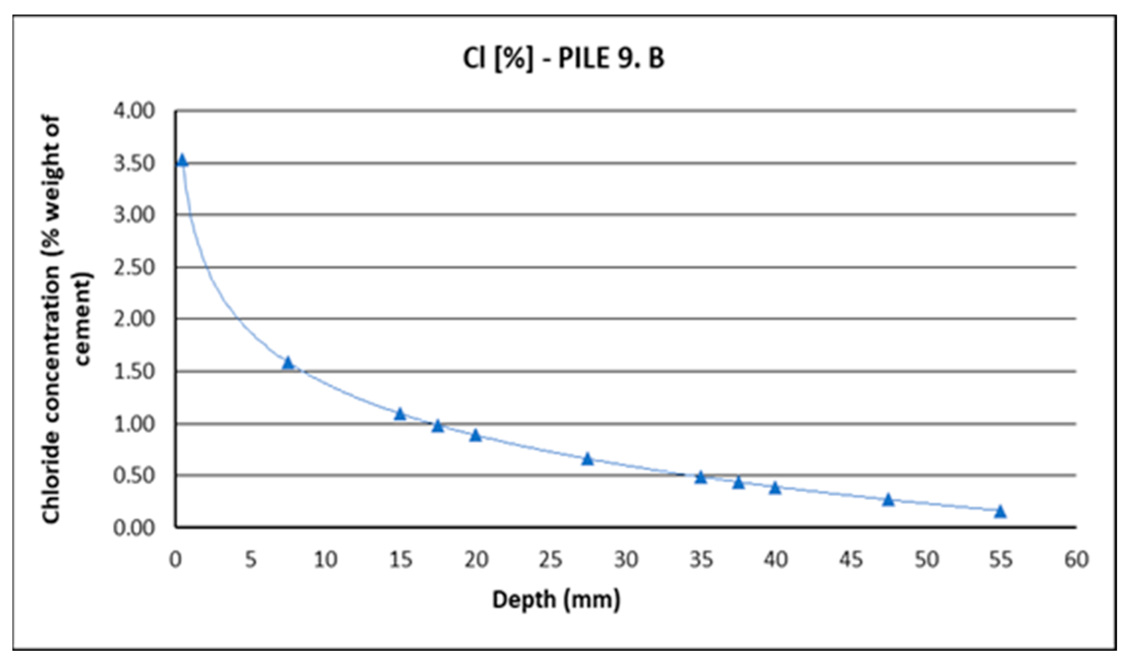
| Structural Elements | Sample Designation and Location | Chloride Content (%) at Each | ||
|---|---|---|---|---|
| Depth (mm) | ||||
| 0–15 | 20–35 | 40–55 | ||
| VIADUCT PILES | T-32 Pile 2 | 0.08 | 0.08 | 0.08 |
| T-33 Pile 2 | 0.49 | 0.20 | 0.14 | |
| T-34 Pile 3 | 0.57 | 0.39 | 0.26 | |
| T-35 Pile 3 | 2.20 | 1.93 | 0.38 | |
| T-41 Pile 3 | 1.65 | 0.46 | 0.41 | |
| T-23 Pile 2 | 0.62 | 0.42 | 0.23 | |
| T-38 Pile 2 | 3.05 | 2.82 | 0.70 | |
| T-39 Pile 1 | 1.99 | 1.70 | 0.57 | |
| Calculation of the Initiation Period (Years) | ||
|---|---|---|
| Parameter | Source | Data |
| Concrete Cover | Structure documentation | 40 mm |
| Service life of the structure | Structure documentation | 23 years |
| Cement type | Structure documentation | CEM I |
| Porosity | Structure documentation | 13.4% |
| w/c ratio | Based on porosity | 0.5 |
| Table A.9.4 (EHE-08) | 1.58 × 10⁻¹¹ m2/s | |
| Section 1.2.2.2 (EHE-08) | 0.0767 years | |
| n | Section 1.2.2.2 (EHE-08) | 0.5 |
| (% weight cement) | Chloride profiles | 3.53 |
| (% weight cement) | EHE-08 recommendation | 0.6 |
| (% weight cement) | EHE-08 recommendation | 0.4 |
| Reinforcement diameter | Structure documentation | 25 mm |
| (Equation (4)) | 13.88 | |
| Initiation period | (Equation (3)) | 8.30 years |
| Nº | ts (Years) | Initiation Period ti (Years) | Propagation Period tp (Years) = ts–ti |
|---|---|---|---|
| 1 | 38 | 11.39 | 26.61 |
| 2 | 35 | 18.60 | 16.40 |
| 3 | 35 | 3.95 | 31.05 |
| 4 | 35 | 3.49 | 31.51 |
| 5 | 35 | 4.40 | 30.60 |
| 6 | 45 | 11.81 | 33.52 |
| 7 | 35 | 7.14 | 27.86 |
| 8 | 35 | 2.79 | 32.21 |
| 9 | 35 | 3.11 | 31.89 |
| 10 | 35 | 3.11 | 31.89 |
| 11 | 35 | 8.89 | 26.11 |
| 12 | 35 | 3.55 | 31.45 |
| 13 | 63 | 2.84 | 60.16 |
| 14 | 63 | 7.36 | 55.64 |
| 15 | 63 | 8.09 | 54.91 |
| 16 | 63 | 6.87 | 56.13 |
| 17 | 63 | 12.09 | 50.91 |
| 18 | 18 | 9.54 | 8.46 |
| 19 | 18 | 10.15 | 7.85 |
| 20 | 18 | 9.82 | 8.18 |
| 21 | 37 | 10.90 | 26.10 |
| 22 | 37 | 15.87 | 21.13 |
| 23 | 37 | 9.11 | 27.89 |
| 24 | 37 | 17.86 | 19.14 |
| 25 | 23 | 16.63 | 6.37 |
| 26 | 23 | 8.30 | 14.70 |
| 27 | 23 | 5.23 | 17.77 |
| 28 | 23 | 5.71 | 17.29 |
| 29 | 36 | 24.02 | 11.98 |
| 30 | 36 | 10.18 | 25.82 |
| 31 | 36 | 10.42 | 25.58 |
| 32 | 36 | 9.17 | 26.83 |
| Nº | Real Diameter Loss Pr (mm) | Diameter Loss Liu & Weyers Px (mm)-Equation (2) | Safety Factor Px/Pr |
|---|---|---|---|
| 21 | 1.20 | 1.493 | 1.24 |
| 22 | 0.60 | 0.856 | 1.43 |
| 23 | 0.60 | 1.788 | 2.98 |
| 24 | 0.80 | 1.281 | 1.60 |
| Nº | Real Diameter Loss Pr (mm) | Diameter Loss Liu & Weyers Px (mm)-Equation (2) | Safety Factor Px/Pr |
|---|---|---|---|
| 6 | 5.10 | 9.408 | 1.84 |
| 3 | 4.00 | 4.988 | 1.25 |
| 4 | 4.00 | 4.667 | 1.17 |
| 5 | 4.00 | 5.511 | 1.38 |
| 8 | 3.60 | 3.884 | 1.08 |
| 13 | 6.25 | 11.575 | 1.85 |
| 14 | 5.00 | 7.157 | 1.43 |
| 16 | 9.00 | 11.534 | 1.28 |
| 17 | 5.00 | 9.469 | 1.89 |
| 18 | 1.00 | 1.486 | 1.49 |
| 19 | 1.50 | 2.105 | 1.40 |
| 20 | 1.00 | 3.200 | 3.20 |
| 21 | 1.20 | 5.373 | 4.48 |
| 22 | 0.60 | 6.462 | 10.77 |
| 23 | 0.60 | 6.027 | 10.05 |
| 24 | 0.80 | 3.396 | 4.25 |
| 26 | 0.50 | 4.083 | 8.17 |
| 29 | 2.10 | 2.155 | 1.03 |
| Nº | Real Diameter Loss Pr (mm) | Diameter Loss Li (2004) Px (mm)-Equation (2) | Safety Factor Px/Pr |
|---|---|---|---|
| 6 | 5.10 | 7.540 | 1.48 |
| 3 | 4.00 | 6.903 | 1.73 |
| 4 | 4.00 | 7.022 | 1.76 |
| 5 | 4.00 | 6.788 | 1.70 |
| 8 | 3.60 | 7.202 | 2.00 |
| 9 | 4.00 | 7.119 | 1.78 |
| 10 | 4.00 | 7.119 | 1.78 |
| 11 | 5.00 | 5.650 | 1.13 |
| 13 | 6.25 | 14.736 | 2.36 |
| 14 | 5.00 | 12.179 | 2.44 |
| 15 | 6.25 | 13.278 | 2.12 |
| 16 | 9.00 | 13.615 | 1.51 |
| 17 | 5.00 | 13.480 | 2.70 |
| 18 | 1.00 | 1.505 | 1.50 |
| 20 | 1.00 | 1.446 | 1.45 |
| 21 | 1.20 | 5.648 | 4.71 |
| 22 | 0.60 | 4.420 | 7.37 |
| 23 | 0.60 | 6.099 | 10.16 |
| 24 | 0.80 | 3.939 | 4.92 |
| 25 | 2.00 | 2.893 | 1.45 |
| 26 | 0.50 | 1.071 | 2.14 |
| 27 | 3.00 | 3.612 | 1.20 |
| 29 | 2.10 | 2.274 | 1.08 |
| 30 | 2.70 | 5.578 | 2.07 |
| 31 | 5.00 | 5.518 | 1.10 |
| 32 | 4.00 | 5.831 | 1.46 |
| Nº | Real Diameter Loss Pr (mm) | Diameter Loss Liu and Weyers Px (mm)–Equation (2) | Safety Factor Px/Pr |
|---|---|---|---|
| 12 | 10.00 | 11.270 | 1.13 |
| 13 | 6.25 | 12.885 | 2.06 |
| 15 | 6.25 | 21.462 | 3.43 |
| 16 | 9.00 | 7.287 | 1.19 |
| 17 | 5.00 | 10.697 | 1.46 |
| 18 | 1.00 | 1.311 | 1.31 |
| 21 | 1.20 | 1.637 | 2.21 |
| 22 | 0.60 | 1.325 | 2.91 |
| 23 | 0.60 | 1.749 | 1.75 |
| 24 | 0.80 | 1.094 | 1.37 |
| Nº | Real Diameter Loss Pr (mm) | Diameter Loss New Model Px (mm) | Safety Factor Px/Pr |
|---|---|---|---|
| 18 | 1.00 | 1.118 | 1.12 |
| 20 | 1.00 | 1.031 | 1.03 |
| 21 | 1.20 | 2.199 | 1.83 |
| 22 | 0.60 | 1.389 | 2.31 |
| 23 | 0.60 | 2.558 | 4.26 |
| 24 | 0.80 | 1.901 | 2.38 |
| 26 | 0.50 | 0.571 | 1.14 |
| Corrosion Rate Model | Number of Positive Cases | Study Case |
|---|---|---|
| Liu & Weyers (1998) | 1 | 24 |
| Kong et al. (2006) | 0 | 0 |
| Vu & Stewart (2000) | 1 | 24 |
| Li (2004 a) | 3 | 11, 24, 32 |
| Li (2004 b) | 1 | 24 |
| New Empirical Model (Lu et al., 2019) | 1 | 24 |
Publisher’s Note: MDPI stays neutral with regard to jurisdictional claims in published maps and institutional affiliations. |
© 2022 by the authors. Licensee MDPI, Basel, Switzerland. This article is an open access article distributed under the terms and conditions of the Creative Commons Attribution (CC BY) license (https://creativecommons.org/licenses/by/4.0/).
Share and Cite
Vázquez, K.; Rodríguez, R.R.; Esteban, M.D. Corrosion Prediction Models in the Reinforcement of Concrete Structures of Offshore Wind Farms. J. Mar. Sci. Eng. 2022, 10, 185. https://doi.org/10.3390/jmse10020185
Vázquez K, Rodríguez RR, Esteban MD. Corrosion Prediction Models in the Reinforcement of Concrete Structures of Offshore Wind Farms. Journal of Marine Science and Engineering. 2022; 10(2):185. https://doi.org/10.3390/jmse10020185
Chicago/Turabian StyleVázquez, Kerman, Raúl Rubén Rodríguez, and M. Dolores Esteban. 2022. "Corrosion Prediction Models in the Reinforcement of Concrete Structures of Offshore Wind Farms" Journal of Marine Science and Engineering 10, no. 2: 185. https://doi.org/10.3390/jmse10020185