An Improved Ship Weather Routing Framework for CII Reduction Accounting for Wind-Assisted Rotors

Abstract

With the increasingly strict regulations for the energy-saving and emission-reduction technology of ships, minimizing fuel cost and thus reducing the carbon intensity index (CII) is one of the most critical issues in the design and operation of merchant ships. More recently, many wind-assisted devices, such as rotors, wind sails, etc., have been investigated and designed to utilize renewable wind energy. With the equipment of wind-assisted rotors, the optimization of ship routes becomes more important because the effect of this wind-assisted device highly depends on the local wind field along the shipping route. In this paper, an improved ship weather routing framework based on the A* algorithm has been proposed to determine the optimal ship route and ship operations with wind-assisted rotors. The proposed framework effectively utilizes different sources of data, including ship design, weather forecasting and historical sailing information, to produce a better estimation of fuel consumption under the effect of sea states. Several improvements on the classic A* algorithm, including directed searching and three-dimensional extension, are proposed to improve the routing effect and efficiency. Finally, the proposed method was applied to test cases of a VLCC operating from China to the Middle East and the results show that the total fuel consumption could be reduced compared to the minimum distance route.

1. Introduction

Due to the increasing attention on ocean environment protection, many measures have been put forward to reduce greenhouse gas emissions, improve energy efficiency and reduce fuel consumption. The Maritime Environment Protection Committee (MEPC) in International Maritime Organization (IMO) at MEPC 78 (June 2022) has discussed and adopted a series of guidelines [1,2,3,4] for short-term measures, including the revised Ship Energy Efficiency Management Plan (SEEMP) and the Carbon Intensity Indicator (CII) coefficient revision. CII is a new method to measure CO₂ emissions from ship operations. In terms of ship operations, CII will be used as an indicator to characterize the actual operational energy efficiency level of ships. In addition, as an indicator of the operational carbon intensity of ships, CII will also be used to measure whether shipping greenhouse gas emissions meet the requirements of the IMO preliminary strategy. After the enforcement of these rules, the attained CII of a ship will be calculated based on the data collected throughout the previous calendar year, and the CII grade for the current year shall be determined based on the CII discount rate. The CII grades are A–E, and ships that have received grade E for one year or grade D for three consecutive years must propose a plan to improve their grade and record it in SEEMP.

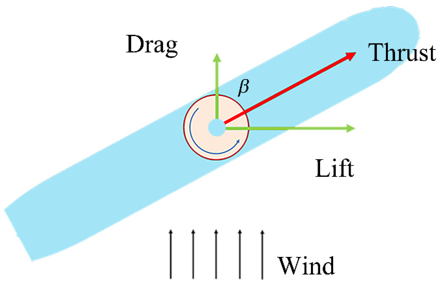
In recent decades, various new concepts of Energy Saving Devices (ESDs) and innovative hull forms have been developed in improving the overall propulsion efficiency to meet the increasingly restrictive EEDI requirements [2]. As the traditional efforts on hydrodynamic energy saving is gradually reaching their limit, some innovative Energy-Saving Devices such as wind-assisted rotors and wind sails were adopted and equipped on ship decks to produce additional thrust. These types of ESDs are more dependent on the weather condition, thus the selection of ship routes will directly affect the effectiveness of these devices.

Ship weather routing is an efficient way to help improve the ship’s operational efficiency and reduce the shipping cost from the view of an economic long-term voyage. The underlying purpose of this economical ship routing is to establish the optimum path and operational profile for the long-distance voyage, as the shortest route is not always the fastest or the most economical way due to the effect of various sea states. Traditionally, the ship’s route is determined by the captains based on their experience and personal capability. This could be improved with advanced technologies included in the Integrated Bridge System such as Electronic Chart Display and Information Systems (ECDISs) which could obtain real-time weather forecasts data, display ship and environment information and provide route planning [5]. There are numerous methods, programs and software that have been developed and equipped on ships in operation. The core algorithms for these methods could be simply divided into two categories [6]: cell-based methods and cell-free methods. The cell-based methods require a discretization of the sea chart and generate the ship’s path by searching the discrete cells. The most widely used cell-based methods are the A* algorithm [7,8] and the Dijkstra algorithm [7]. The latter one is the most classic path-routing algorithm based on graph theory and the A* algorithm is an advanced version of the Dijkstra algorithm that introduces the greedy property to improve the searching efficiency. For better speed planning in weather routing, a 3D Dijkstra optimization algorithm [9] was also proposed to generate globally optimal ship routes that encounter less harsh offshore environments and reduce fuel consumption. Some other modifications are also proposed to improve different applications such as greenhouse gas emission control [10]. Cell-free methods are derived from the classical routing practices in navigation. The main idea of the currently developed cell-free method derives from the classical way of ship routing based on conventional paper charts such as the isochrone method. For example, the classic isochrone method [11] proposed by Hanssen and James could determine an economical route but has some difficulty with voyages with many obstacles. Some improvement [8] has been made to solve this problem and was extensively applied to the simultaneous determination [6] of ship routes. Recently, an improved method [10] that considered the advantages and disadvantages of both cell-based methods and cell-free methods was proposed to improve the cell-based path planning algorithm for the generation of optimal weather routes. Meanwhile, comprehensive software for ship weather routing is designed [12] where the wave condition is taken as the optimization objective, and the A* algorithm is used to achieve the optimal route generation. On the other hand, the cell-free method is not confined by the discretization of a sea chart and could make a continuous search of all directions and positions. Roh overviewed the most widely used ship-routing methods and proposed an improved version with the consideration of obstacles [13]. The 3D dynamic programming algorithm [14] is also a cell-free method that could generate an optimal path and speed profile. In addition to the above two categories, many studies transform the weather route-planning problem into an optimization problem for solving. In study [15], a ship meteorological route path-optimization algorithm based on a multi-objective genetic algorithm was proposed by considering ship characteristics and rough weather conditions. With the minimization of total voyage time and total fuel consumption as the optimization objective, the optimal route and speed are realized. Some evolutional methods such as the improved ant colony algorithm were introduced to improve the convergence speed and avoid the local optimum for a ship’s weather path generation [16]. The result shows that the optimized route planned by the algorithm can avoid dangerous areas in the term of the voyage and ensure the safety of the ship at sea. In addition, based on the original fractional order particle swarm optimization algorithm, the new coefficients of the fractional order velocity update formula are improved to avoid falling into local optimization [17]. On this basis, the ship weather route of a VLCC tanker is optimized with the minimum fuel consumption.

Another important issue in weather routing is the estimation of total fuel consumption (TFOC) among sea states. As the performance of the ship changes with sea states, the total resistance will increase in severe sea states with high waves, and thus, ship speed will reduce with the same engine power compared with still water conditions. Additionally, with the equipment of wind-assisted rotors, the rotor system will produce a favorable thrust in sea states with a strong side wind. The estimation of total fuel consumption should consider both wave-added resistance [18,19] and rotor-added thrust [20] and then help to generate the most efficient path and operation file. The TFOC could be estimated according to theory-based or practice-based methods [6]. Roh [8] established a method for estimating fuel consumption by calculating the horsepower compensation due to a bad sea state following the theory-based method of ISO 15016 [21]. On the other hand, Lee et al. utilize a practice-based method with past ship-operation data. This is an easy-to-use way with the help of a nonlinear multiple regression model. In recent years, with the development of big data, artificial intelligence technologies and machine learn-based methods have been widely used in ship fuel consumption estimation. Many studies have applied the black box model of neural network to the prediction of shipping fuel consumption [22,23,24,25,26,27]. Based on the noon report data and automatic monitoring data, such as support vector machine, random forest, extra tree regression and artificial neural networks, and concluded that random forest and extra tree had the best prediction performance [22]. Similarly, BP neural network, deep belief network, K-nearest neighbor, decision tree and support vector regression were used to establish ship fuel consumption prediction models, and the applicability and advantages of these algorithms were explained in detail [24]. Taking wind speed, draft, water velocity, rudder angle and ship speed as input parameters, an artificial neural network model could be applied for fuel consumption prediction based on the measured sailing data [25]. Additionally, methods combining artificial neural networks and multiple regression are widely used to estimate the power and fuel consumption of ships [26], and it could better realize the real-time prediction and is more adaptive to possible changes in the ship environment. In addition, a more systematical forecasting framework [27] for ship fuel consumption based on the least absolute shrinkage and selection operator regression algorithm is a new trend.

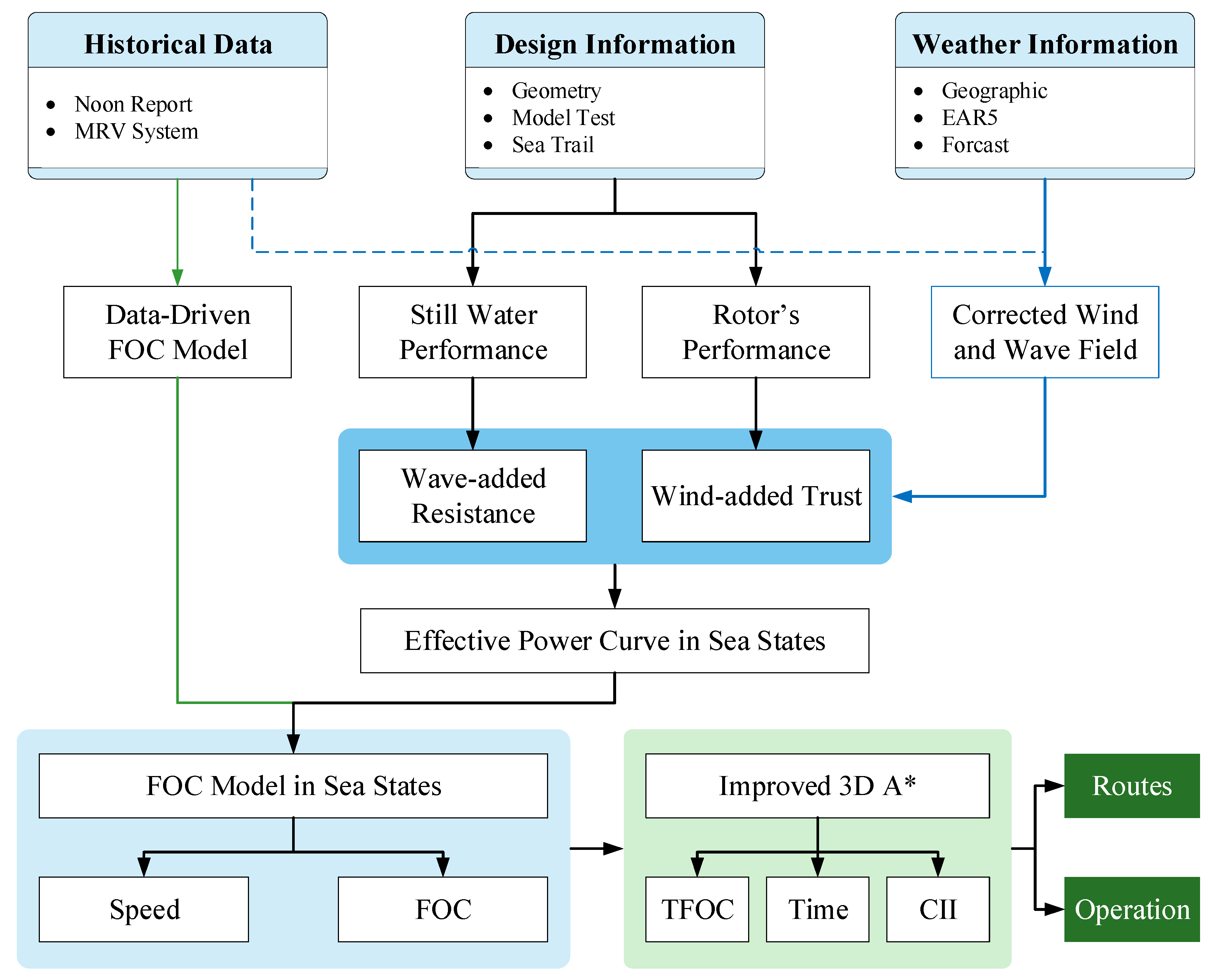
In this paper, an improved ship weather routing framework towards low carbon shipping and CII reduction is proposed based A* algorithm and complex FOC estimation models. This article is organized as follows: Section 2 gives the main methodology, including data-acquisition, improvement of the classic A* algorithm and estimation methods for fuel consumption and CII. A detailed analysis based on a VLCC ship from China to the Middle East is provided in Section 3 to illustrate the effect of the proposed methods. In Section 4, a short conclusion is presented and a plan for future research is given.

2. Methodology

2.1. Problem Definition

For the navigation of ocean-going commercial vessels, the theoretically shortest path is the great circle route from spherical trigonometry. For better sailing decisions in complicated natural geographical environments, weather conditions and dynamic navigation circumstances, improved routing strategy and decision-making software shall be developed, incorporating the control of novel energy-saving devices such as wind-assisted rotors.

The main task of improved weather routing in this article is to find the optimal path and optimal operation profile based on weather information, the ship’s basic design performance and historical sailing data of similar ships. The optimal path consists of a series of ship heading and voyages, and the operation profile should give the suggested ship speed (or main engine RPM) in every voyage. Compared to the conventional ship routing problem, there are some changes with the consideration of wind-assisted rotors. Rotors’ air-dynamic properties should be included in the estimation of TFOC and dynamic CII which highly depend on ship heading and wind direction. The resultant operation profiles should contain the direction and speed of the rotors’ rotation. Therefore, the improved weather-routing method in this paper consists of three basic parts:

• Acquisition and the pre-process of the environment and ship information.
• Estimation of the ship’s fuel consumption and CII considering wind-assisted rotors.
• Optimization of the ship’s path and operational profile.

With sufficient environment data and the appropriate TFOC estimation model, the weather-routing problem could be defined as an optimization problem with object functions, design variables and constraints. As shown in Equation (1) the objective function is the TFOC of the whole voyage which depends on the design variables including route R, ship speeds V_S and rotor spinning ratio $\alpha$.

$$\mathrm{Minimize} \mathrm{TFOC} \left(R,V_s, \alpha \right)$$

(1)

$$\mathrm{Subject} \mathrm{to} \left\{\begin{array}{l}{t}_{estimated}-t_{required}\le 0\\ Q\le Q_{max}\\ {\theta }_{i-1}-\sigma <{\theta }_i<{\theta }_{i-1}+\sigma \end{array}\right.$$

(2)

where $Q$ is the shaft torque of ship and $Q_{max}$ represents the maximum torque limited by the main engine, which depends on ship types and the selection of the main engine; $\theta$ is the rudder angle and $\sigma$ refers to the change limitation of the rudder angle.

Three additional constraints are applied in this study including required voyage time, maximum torque and heading angle change. First, the ship should arrive at the destination before the latest time, that is the $t_{estimated}$ should be less than the $t_{required}$. Then, in case of safety, the torque of the main engine should not exceed the security boundary according to the standard. In addition, the change of heading angle is constrained to a limited degree $\sigma$.

Compared with previous studies, the estimation of TFOC should consider the effect of wind-assisted rotors. The additional thrust generated by rotors in a positive wind environment could compensate for the energy lost due to bad sea states. Thus, the optimal rotation speed of rotors should be selected in every ship voyage and their effect on TFOC should be considered. Additionally, it should be noted that the solution to the weather-routing problem is a long-term and large-scale path planning and operation optimization problem. Thus, the simultaneous effect of the ship’s motion on rotors or rotors’ effect on the ship’s acceleration of motion is not considered in this paper. The whole framework provided in Figure 1 is based on the statistical perspective with a small-scale effect filtered all over the voyage.

2.2. Data Acquisition and Pre-Processing

As shown in Figure 1, an efficient weather-routing system requires the ship’s design information and weather information for path planning and voyage optimization. Additionally, if any historical sailing data is available for the current ship or similar ships, the data-driven method could be used to improve the FOC and CII estimation for better routing.

2.2.1. Ship’s Design Information

For a ship with wind-assisted rotors, the basic ship design information consists of the ship’s calm water resistance, propulsion performance, main engine profile and rotor’s air dynamic performance. The ship’s resistance and propulsion performance could be obtained from the towing tank test and the rotor’s air dynamic performance comes from the wind tunnel test or a numerical simulation for different designs. These basic design data could provide a baseline for the estimation of fuel consumption and the effect of energy saving from wind-assisted rotors in complex ocean environments.

In this paper, a Very Large Crude Carrier (VLCC) with complete model test data, sea trail data and noon report data on sailing is under investigation. The principal dimensions of the ship and wind-assisted rotors are listed in

Table 1. Principal dimensions of the VLCC.

Items	Description	Value
$L_{PP}$ [m]	Length between the perpendiculars	332.6
B [m]	Beam	60
T [m]	Design draft	20.5
$\nabla$[m3]	Displacement	318,250.3
Nrotor	Number of rotors	6
Drotor [m]	Diameter of rotor	5
Hrotor [m]	Height of rotor	30

. Six wind-assisted rotors with a height of 30 m and a diameter of 5 m were designed for this ship. The ship’s performance in calm water including effective power and delivery power is achieved by model test from the towing tank of China Ship Scientific Research Center (as shown in Figure 2). Figure 3 gives the openwater performance curve of the propeller along with the lift and drag coefficients of wind-assisted rotors according to our numerical simulation. Thus, the powering change in real sea state due to waves and winds could be calculated by our prediction model and the overall fuel oil consumption could be obtained according to the SFOC curve (Figure 2) of the main engine.

2.2.2. Weather Information

Weather routing needs the ocean geographic and ocean weather information to optimize the best route path and operation profile. The geographic data could be obtained from the ECDIS system or other electronic chart data sources. As a cell-based path-planning method will be used in this paper, a rasterization step is, firstly, performed with variable grid resolution to generate computational mesh for the routing algorithm. As shown in Figure 4, a grided mesh is generated according to the given longitudinal and latitudinal resolution. If the center of each grid cell locates in the polygon of land or an island, this cell will be labeled 0 or labeled 1 which means it is accessible for ships. It could be figured out that the resolution of the grid will affect the resultant path from P0 to Pn and this weakness will be reduced by improving the resolution of the grid. Figure 5 shows the computational grid generated from a real geographic map with a spatial resolution of 0.1° for both longitudinal and latitudinal directions.

The ocean climate and weather information including the wave, wind and current is another essential prerequisite for weather routing, along with geographical information. For better routing, both real-time weather forecast data and historical climate re-analysis data are required for modeling and optimization. In this paper, the most recent and widely used reanalysis dataset ERA5 from the European Center for Medium-range Weather Forecasts (ECMWF) is used. ERA5 is the fifth generation ECMWF atmospheric reanalysis of the global climate covering the period from January 1950 to the present and could provide an hourly estimation of a large number of atmospheric, land and oceanic climate variables, including 10 m wind speed, 10 m wind direction, mean wave height, mean wave direction and mean wave period. The weather data acquired from ECMWF is coarse and will be interpolated to the computational grid worldwide to compute wind- and wave-added resistance and FOC in path planning (Figure 6). As can be seen in Figure 7, the significant wave height and wind distributions on the north Pacific Ocean for three continuous days from 1 November 2020 have obvious differences. Thus, instantaneous real-time path planning and voyage optimization shall be performed day-by-day to predict, assimilate and optimize the route.

2.2.3. Historical Sailing Information

Historical sailing data, such as on-board monitoring data or noon report data, is an important complement for hydrodynamic modeling, FOC modeling and data calibration. Ideally, all required on-board data should be correctly and timely monitored through distributed sensors for a highly intelligent ship. However, the most available historical sailing data for ships in operation is the noon report data collected every day at noon artificially or automatedly. Thus, the noon report data is not continuous data that reflect the hourly change of sea states and the ship’s response.

The most useful data for modeling and navigation is the navigational data and main engine’s data, including the ship’s speed over ground, trajectory, main engine speed, power and fuel consumption. Additionally, the weather information, including the wave, wind and current, could be utilized as a reference because only rough directions and levels are provided based on meteorological stations or even human observation which is not very credible.

Figure 8 shows a VLCC’s noon report data of a single voyage from the port of Basrah, Iraq to Zhoushan, China. Variables such as ship speed and main engine RPM have an instantaneous value at 12:00 am every day and variables like fuel consumption and traveling distance have a cumulated amount from 12:00 am the last day. As shown in Figure 9, the main engine power is linearly related to the third power of RPM which is consistent with the model test. However, the relationship between cumulated fuel consumption and RPM is hard to identify. This is mainly because, at every record time, the main engine RPM may change between noon yesterday to the current. The variable weather conditions could have a large effect on the overall fuel consumption.

2.3. Improved A* Algorithm for Ship Weather Routing

The A* algorithm is one of the most popular graph search algorithms that finds the shortest path from the starting point to the target point in a mapped area. A* was developed in 1968 to combine formal approaches such as the Dijkstra algorithm and heuristic approaches like Best-First-Search (BFS). When utilizing the A* algorithm to generate an optimal route for a ship’s operation, a mapped area was, firstly, introduced by discretizing the sea chart. Figure 4 illustrates the representation of sea and land with discrete cells. Then, the path from starting point (P0) to the arrival point (Pn) is represented by a series of connecting lines between cell centers.

The classic A* algorithm used for path routing could not be directly used for the weather-routing problem with both optimal route search and operation optimization tasks. Previous researchers solved this problem by regarding the two tasks separately. They performed path searching with a fixed-speed state and then modify the speed on the path to achieve the optimal operation profile (Park and Kim, 2015; Joo et al., 2012; Bang and Kwon, 2014).

2.3.1. Directed Route Searching

The original route searching strategy of the classic A* algorithm was modified to improve efficiency with higher physical realizability. At each time step, the accessible neighborhoods for next step searching are defined by a vector set $\mathsf{\Omega }$ which consisted of N displacement vectors. In our version, $\mathsf{\Omega }$ will be updated in the real-time path searching according to the ship’s current heading direction instead of a constant vector set for 4 or 8 directions. That is, $\mathsf{\Omega }$ is a function of spatial location X and time t.

$$\mathsf{\Omega }\left(x,t\right)=C^n\cap F\left(\Psi ,\delta ,V\right)$$

(3)

where $C^n$ is the classical constant searching region depending on the layer number n which defines the search range at each step. $F\left(\Psi ,\delta ,V\right)$ is the variable searching region depending on the ship’s heading direction Ψ, rudder angle $\delta$ and ship speed $V$.

As shown in Figure 10, assume that there is a move from P_n to P_n+1 based on the heading direction and the motion characteristics of the vessel. $F\left(\Psi ,\delta ,V\right)$ is defined as a fan-shaped region by searching radius r and heading angel’s changing interval [a, b]. The change of heading angle β must belong to the available range which is determined by the maneuverability of the ship. Regarding the numerical implementation, grid cells in the fan-shaped region will be selected to perform a unit Boolean operation with a constant region $C^n$. For example, assume that n = 1 and radius r = 1.5$\mathrm{\Delta }$, where $\mathrm{\Delta }$ is the grid size, the resultant $\mathsf{\Omega }$ (green cells) and its related directions could be achieved as shown in Figure 11b. A nonsymmetric interval [a, b] is acceptable in situations where the ship’s maneuverability is affected by sea states. Figure 11c,d give the search result with and without obstacles.

2.3.2. Three-Dimensional A* for Speed Optimization

In previous studies, the shortest route planning and speed optimization are always separate steps in weather routing. For ships sailing in severe sea states with wind-assisted rotors, the overall performance of ship and related fuel consumption has a strong relationship with ship speed. In this paper, we would like to incorporate speed optimization with path planning task so that two tasks could be fulfilled in one framework with synchronized evaluation of fuel consumption and CII to achieve the best result. Thus, another improvement is to extend the A* algorithm to a three-dimensional one and the 3rd dimension is defined as ship speed (Figure 12).

As shown in Figure 13, the operation optimization task could be directly achieved by searching the optimal calm water ship speed (equivalent to main engine power). The accessible searching region in speed direction is also predefined to constraints the speed variation. When the optimal route and main engine power are obtained, the operation profile could be achieved by simply interpolating the ship performance curves.

2.3.3. Cost Function and Heuristic Function

As A* is a graph traversal and path-search algorithm which is formulated in terms of a weighted graph, the most important part of its application to different scenarios is to formulate the cost function and heuristic function to be minimized. Specifically, A* selects the optimal path that minimizes

$$f\left(n\right)=\mathrm{g}\left(n\right)+h\left(n\right)$$

(4)

where g(n) is the cost function which defines the cost of the path from the start node to the nth node; $h\left(n\right)$ is a heuristic function that estimates the cost of the optimal path from the current node to the end.

Both the cost function and heuristic function are problem specific. The cost function reflects the real cost from the start node while the heuristic function is an estimation of the future based on the specific greedy strategy. The efficiency of A* will highly depend on the candidate-searching region (defined in the last sub-section) and the selection of the heuristic function. Generally, the Manhaton distance or Euclidean distance are the most widely used for cost function and heuristic function in a shortest path searching problem. For the weather-routing problem in the real world, the Euclidean distance is more appropriate to construct the basis of these two functions. Additionally, modifications based on the TFOC estimation and CII computation are introduced to find the optimal route with a reduction in TFOC and CII.

The cost function with the effect of the sea state is expressed as

$$\left\{\begin{array}{l}g\left(n+1\right)=g\left(n\right)+\mathrm{\Delta }g \\ \mathrm{\Delta }{g}^n=H_w\left(n\right)\mathrm{\cdot }\sqrt{{\left(x_{n+1}-x_n\right)}^2+{\left(y_{n+1}-y_n\right)}^2}\end{array}\right.$$

(5)

where $\mathrm{\Delta }g$ represents the change of ship cost (FOC or CII) in every sailing segment from node n to $n+1$, and $H_w\left(n\right)$ is the state effect coefficient in this sailing segment related to the wave, wind and the resultant engine RPM.

Similarly, the heuristic function is

$$h\left(n\right)=\overline{H_w}\cdot \sqrt{{\left(x_n-x_d\right)}^2+{\left(y_n-y_d\right)}^2}$$

(6)

where $\overline{H_w}$ is the estimated average state effect from the current node to the end related to the predicted wave, wind and resultant engine RPM. Both $H_w\left(n\right)$ and $\overline{H_w}$ are computed in the routing process based on the specific TFOC model and CII computation method described as follows.

2.4. TFOC Estimation and CII Computation

As shown in Figure 1, the resistance change due to sea states could be estimated based on the wave-added resistance, wind resistance and rotor-added thrust. Assuming that the sea state has negligible effect on the self-propulsion factors but has an influence on the propeller’s open water efficiency due to the variation on propeller loading, the reduction in propulsion efficiency could be obtained following the recommendation of ISO 15016. Then, we could have the effective power curve in sea states and the resultant ship speed with a given engine power.

2.4.1. Effect of Wave and Wind

The severe sea state has a negative effect on ship performance due to the wave-added resistance. The resultant ship speed could be reduced, and thus additional power is required to compensate for the speed lost. On the other hand, some sea state with strong side-wind could help the wind-assisted rotors to produce positive thrust and then compensates for the wave-added resistance. With environment information (mainly wave and wind), ship information (ship geometry, engine information and performance curves from experiments) and given operations (ship heading, engine power and rotor speed), we could obtain the wave-added resistance by the 2D strip theory [28], the wind resistance according to an empirical formula (Equation (7)) and the rotor-added thrust by a pre-calculated dataset. Then, the resultant ship speed in the real sea state could be achieved by a calculation code of the ship speed loss coefficient proposed and verified by Wei et al. [12]. The error of estimated speed loss coefficient is less than 3% compared to the experiment result according to their work.

$$R_{wind}=\frac{1}{2}\rho C_x{V}_R^{2}A/1000$$

(7)

where $\rho$ refers to the air density, $C_x$ is the wind resistance coefficient, V_R is the relative wind speed and $A$ is the projected area above the water surface.

2.4.2. Effect of Wind-Assisted Rotors

The rotor-added thrust is produced by the magus effect which generates a sidewise force on a spinning cylindrical when there is relative motion between the spinning body and the fluid (air). The mechanism of the wind-assisted rotors is illustrated in Figure 14. Thus, the thrust on the ship could be calculated by Equation (8).

$${\mathrm{C}}_T={\mathrm{C}}_L\cdot \sin \beta -{\mathrm{C}}_D\cdot \cos \beta$$

(8)

where ${\mathrm{C}}_L$ is the lifting coefficient, ${\mathrm{C}}_D$ is the drag coefficient, ${\mathrm{C}}_T$ is the thrust coefficient and $\beta$ refers to the relative wind angle. All the coefficients are normalized by 1/2$\rho v^{2}S$, where $\rho$ is the density of air, V is the relative speed of wind and S is the projected area of the rotor.

The ${\mathrm{C}}_L$ and ${\mathrm{C}}_D$ rely on the spinning ratio of the rotor which is defined as $\alpha =\frac{\mathsf{\Omega }{D}_{rotor}}{2V}$, where $\mathsf{\Omega }$ is the rotating speed of the rotor and $D_{rotor}$ refers to the rotor diameter. Based on Equations (8) and (9) the correlation between the thrust coefficient and the spinning ratio could be pre-calculated by the CFD method.

$$\left\{\begin{array}{l}{\mathrm{C}}_L=\frac{L}{0.5\rho v^{2}A}\\ {\mathrm{C}}_D=\frac{D}{0.5\rho v^{2}A}\end{array}\right.$$

(9)

RANS solver with SST $k-\omega$ model was applied in this study according to our previous work of Hu et al. [13], where detail information of CFD method, mesh strategy and verification study could be found. Based on the lifting and drag coefficient computed by RANS solver shown in Figure 3 the optimal spinning ratio could be selected with the maximum rotor-added thrust, as shown in Figure 15.

2.4.3. Neural Network Modeling for Real-Time Routing

As the algorithm searches over 100 thousand possibilities in a single optimization procedure, the time consumption of running the 2-D strip program in real-time with the optimization algorithm is unacceptable. Therefore, we introduced a meta-model method based on an artificial neural network to make a fast prediction of wave-added resistance and the resultant ship speed. The dataset for Artificial Neural Network (ANN) training was prepared considering all the possible experienced sea states with the 2-D strip program.

Table 2. Required training data for ANN modeling.

Category	Items	Definition
Training Input	Hwave	Wave height
	Twave	Wave period
	θwave	Wave-approach angle
	Vwind	10 m wind speed
	θwind	Wind-approach angle
	P	Engine Power
Training Output	Vsref	Reference ship speed in calm water
	Vsw	Resultant ship speed in sea state
	Rw	Wave-added resistance
	Ra	Wind resistance

shows the input and output data for the supervised training of the ANN model. A physics-informed Latin Hypercube Sampling method was adopted to generate the pre-calculation samples which means that the input variables are not independent but adaptively sampled according to the distribution of weather forecast data. Over 32,000 sets of training data were pre-calculated with the 2D strip program and ship speed loss calculation so that we could utilize an artificial neural network to build the relationship between the environment information and the resultant ship speed in real sea states. The ANN model consists of 5 hidden layers with a sigmoid activation function and 3 output layers with linear activation function. Figure 16 shows the validation of the trained ANN model on a short route in the west–north Pacific Ocean. The result shows that the physics-informed way of sampling could significantly improve the performance of the ANN model. The minor variation of speed due to sea states change could be captured by the model.

2.4.4. Estimation of Real-Time Fuel Consumption and CII

With given ship power, the resultant ship speed in real sea state could be obtained. Then, the total fuel consumption could be achieved by Equation (10),

$$TFOC={\displaystyle \sum }_{i=1}^{N}SFOC\left(P_i\right)\cdot P_i\cdot t_i={\displaystyle \sum }_{i=1}^N\frac{SFOC\left(P_i\right)\cdot P_i\cdot L_i}{V_i}$$

(10)

where N is the number of voyage segments, $P_i$ and $t_i$ is the averaged engine power and the duration time in every segment. As sailing time $t_i=\frac{L_i}{V_i}$, the sea state effect coefficients $H_w$ equals to

$$H_w\left(n\right)=\frac{SFOC\left(P_n\right)\cdot P_n}{V_n}$$

(11)

where $V_n$ is the average ship speed in node n on computational grid and $P_n$ is its corresponding engine power. As described in our improved A* algorithm, the reference calm water ship speed is selected as an optimization variable and its corresponding engine power is calculated from the ship’s speed–power curve.

According to the CII Guidelines G1 [27], the attained annual operational CII of individual ships is calculated as the ratio of the total mass of CO₂ (M) emitted to the total transport work (W) undertaken in a given calendar year, as follows:

$$Attained CII=M/W$$

(12)

The total mass of CO₂ is the sum of CO₂ emissions (in grams) from all the fuel oil consumed on board a ship in a given calendar year, as follows:

$$M=\sum F{C}_j\times C_{Fj}$$

(13)

where j is the fuel oil type; $F{C}_j$ is the total mass (in grams) of consumed fuel oil of type in the calendar year; $C_{Fj}$ represents the fuel oil mass to CO₂ mass conversion factor for fuel oil type, in line with those specified in the 2018 Guidelines on the method of calculation of the attained Energy Efficiency Design Index (EEDI) for new ships [28], and may be further amended. In case the type of fuel oil is not covered by the guidelines, the conversion factor should be obtained from the fuel oil supplier supported by documentary evidence, detailed information could be found in the MEPC guidelines.

For the weather-routing problem, the supply-based transport work (W) can be taken as a proxy in the absence of data in actual transport work. The transport work is calculated as the product of a ship’s capacity (C) and the distance traveled ($D_t$) according to the MPEC guidelines, that is

$$W=C\cdot D_t$$

(14)

3. Applications

The optimization method proposed in this paper was applied to the VLCC test case. In the route optimization procedure, the increase in ship resistance in the sea state will certainly change the powering curve and thus, lead to the reduction in ship speed while the existence of the rotor system will compensate for this.

We simulate the ship-routing problem for a VLCC from China to the Middle East for oil trade. This route makes its way through the East China Sea, the South China Sea, Singapore, the Indian Ocean and the Strait of Hormuz. A typical characteristic ff the Indian Ocean route is the strong side-wind which is positive to the wind-added rotors. Similarly, five routes were generated by the proposed algorithm with different weather, power and rotor considerations. To analyze the effect of different method combinations, 30 cases for every combination are simulated based on different dates of departure to achieve a statistical result of routing. The meaning of the keywords for different method selections in column 2 of

Table 3. Averaged routing results for 30 cases per method combination.

NO	Method Combination	TFOC	Voyage Time	CII
MC1	Shortest Route	100%	100%	100%
MC2	Weather	95.39%	100.47%	93.11%
MC3	Weather, Speed Optimization	84.78%	108.51%	82.53%
MC4	Weather, Speed Optimization, Rotors	80.37%	101.9%	78.63%

are listed for better understanding:

• Shortest Route: Only the shortest path searching based on the Euclidean distance is applied;
• Weather: Weather routing considering the effect of the wave and wind;
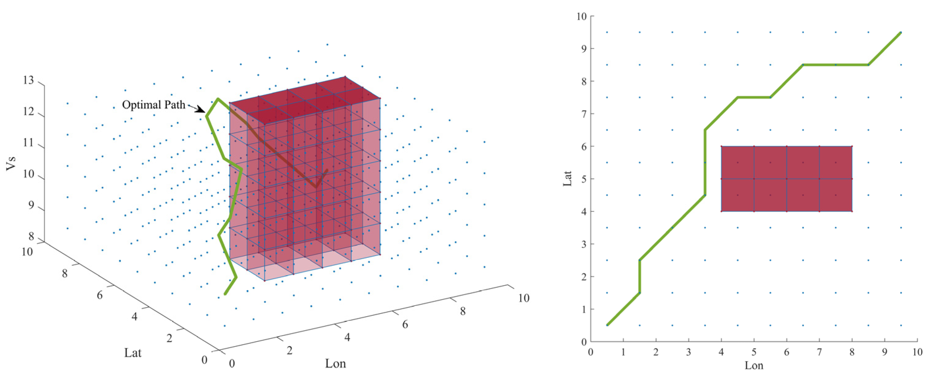
• Speed Optimization: The 3D A* algorithm is activated to optimize the engine delivery power to achieve the optimal ship speed;
• Rotors: The effect of wind-assisted rotors is considered.

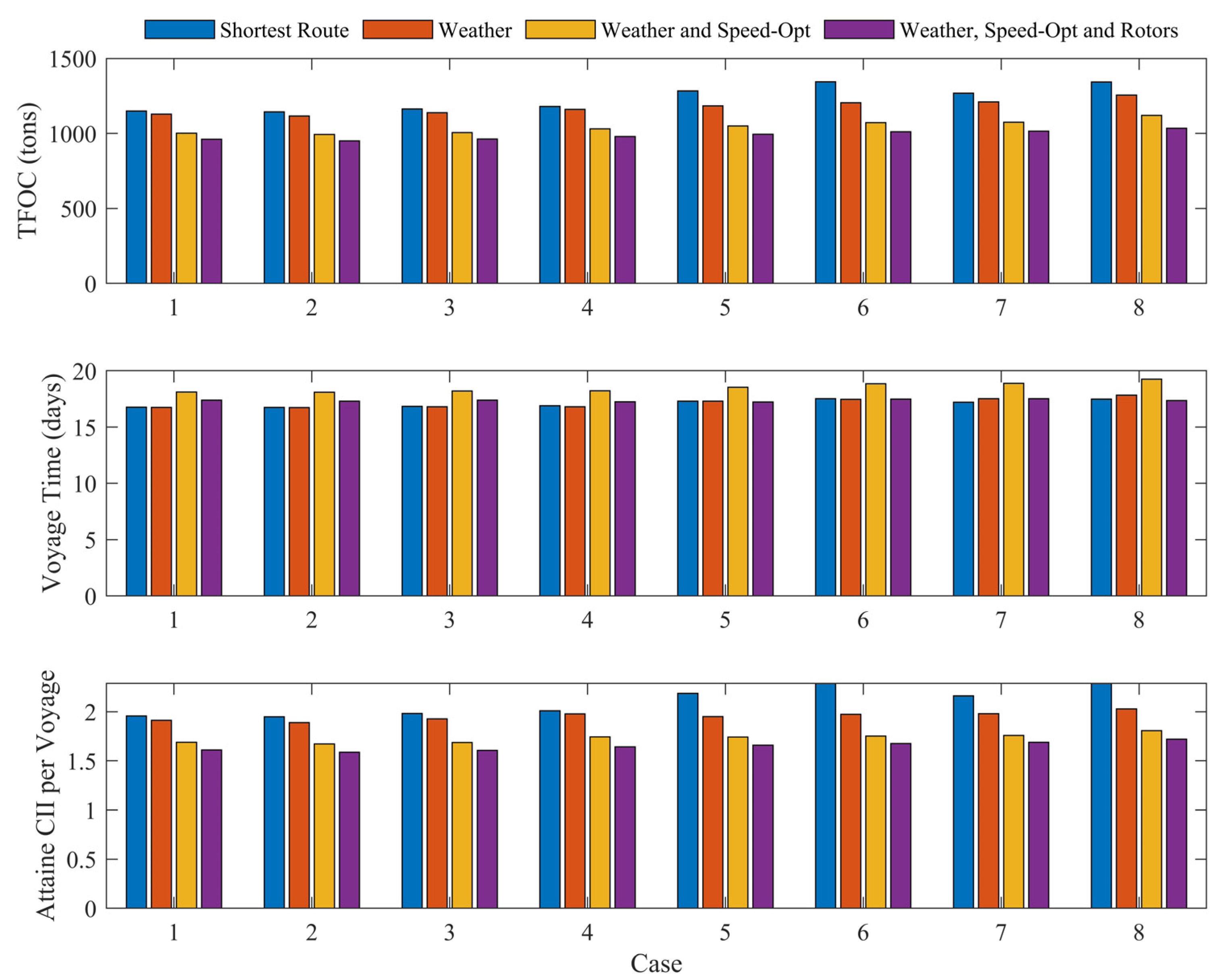
Table 3 summarizes the averaged routing results over 30 cases per method and object combination and the results of eight selected cases are shown in Figure 17. It could be figured out that weather routing could provide a 4.61% reduction in TFOC and a 8.89% reduction in CII on this voyage with almost the same voyage time. Further, the speed optimization in a preassigned range could provide a 10.61% additional reduction in TFOC and 10.58% of CII, respectively. On this basis, with the help of wind-assisted rotors, the joint optimization of routes, speed and rotor operation speed could contribute an additional 4.41% reduction in TFOC and 3.90% of CII. As shown in Figure 17, for different cases with different ocean weather conditions, the fuel consumption, voyage time and attained CII have great differences but the contributions from different routing techniques are similar. Due to the third power relationship between the ship’s speed and delivery power, speed optimization always contributes the most part to the TFOC and CII reduction and always leads to a lower average speed, and thus a longer voyage time.

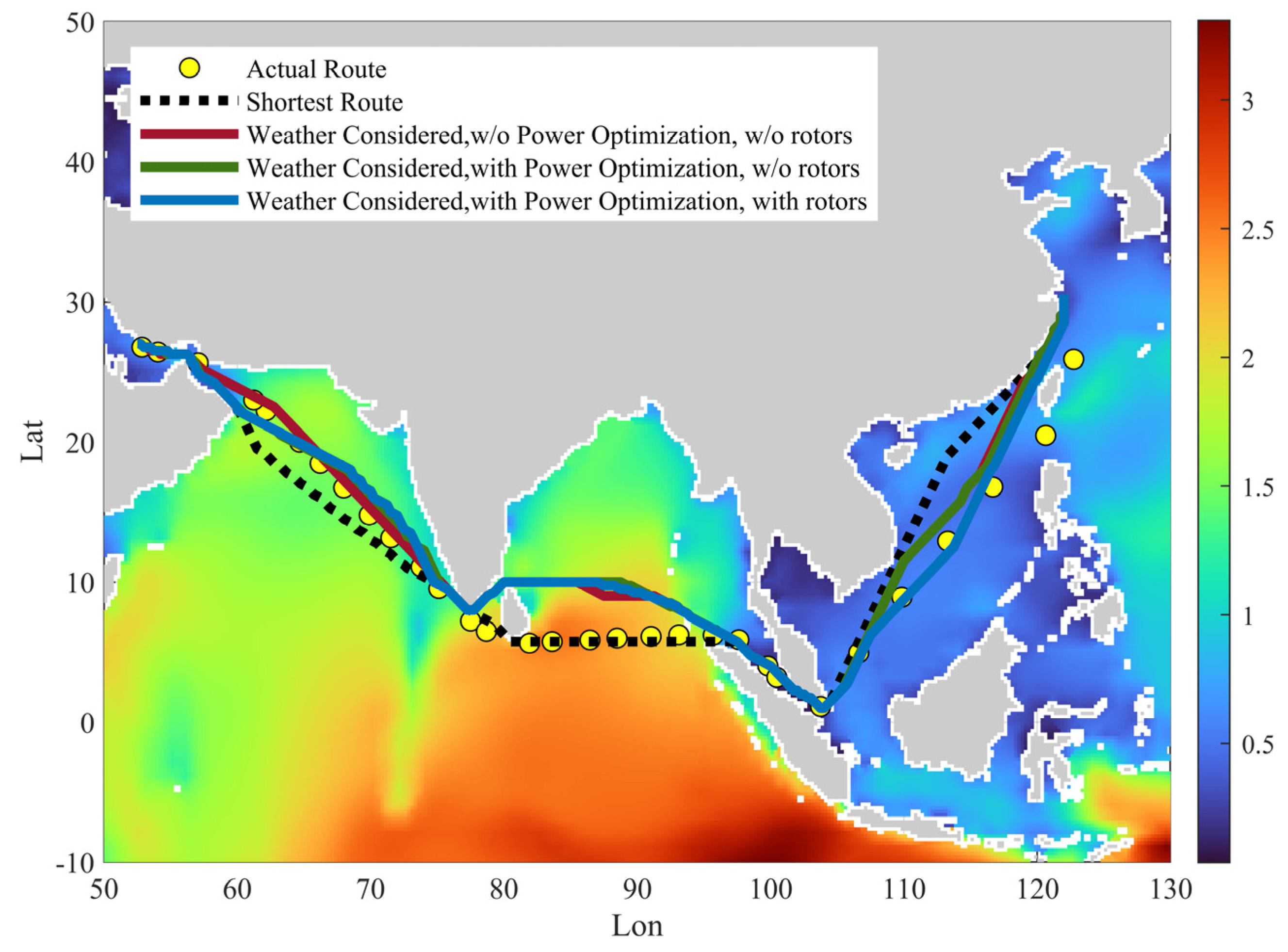
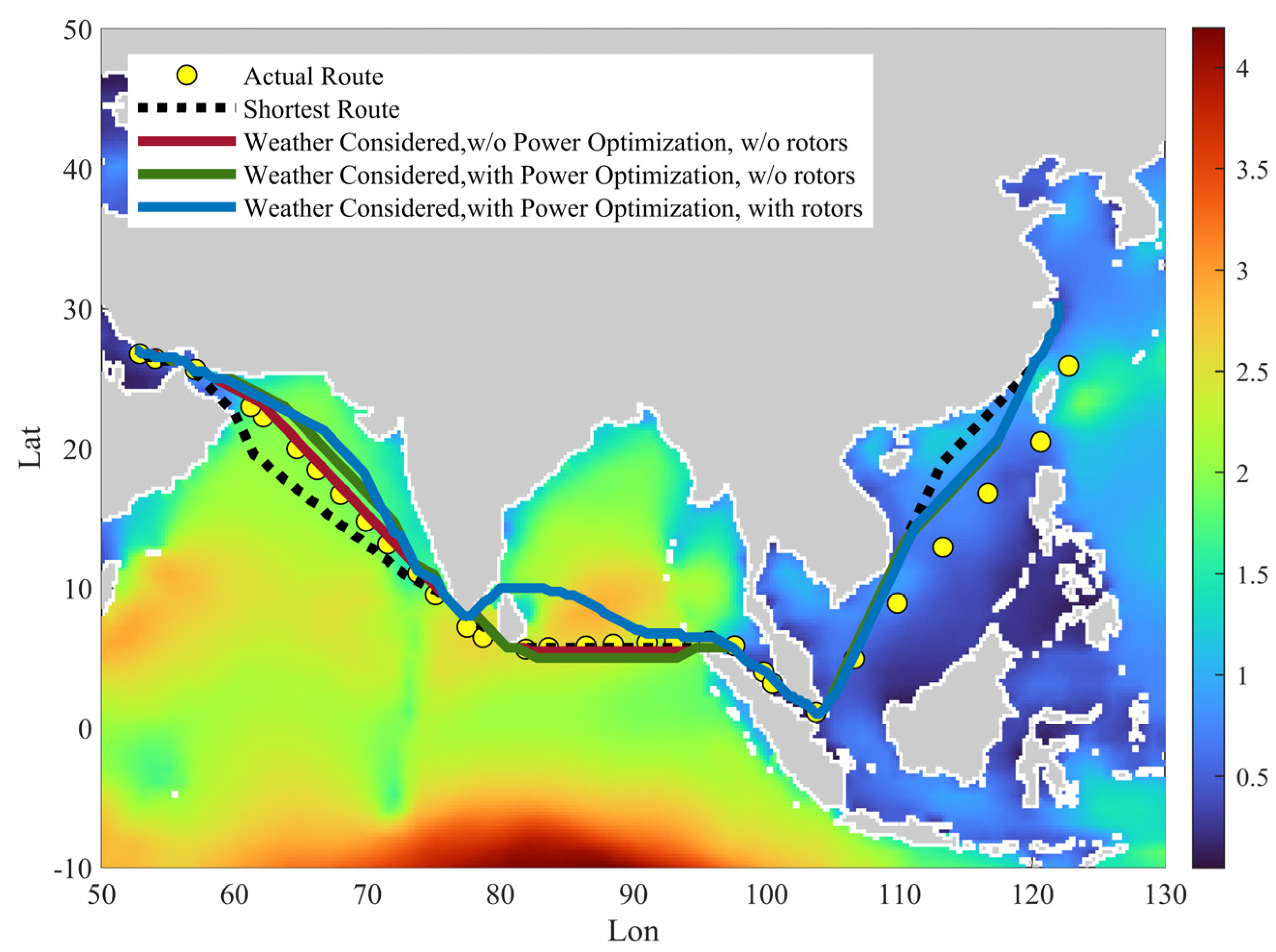
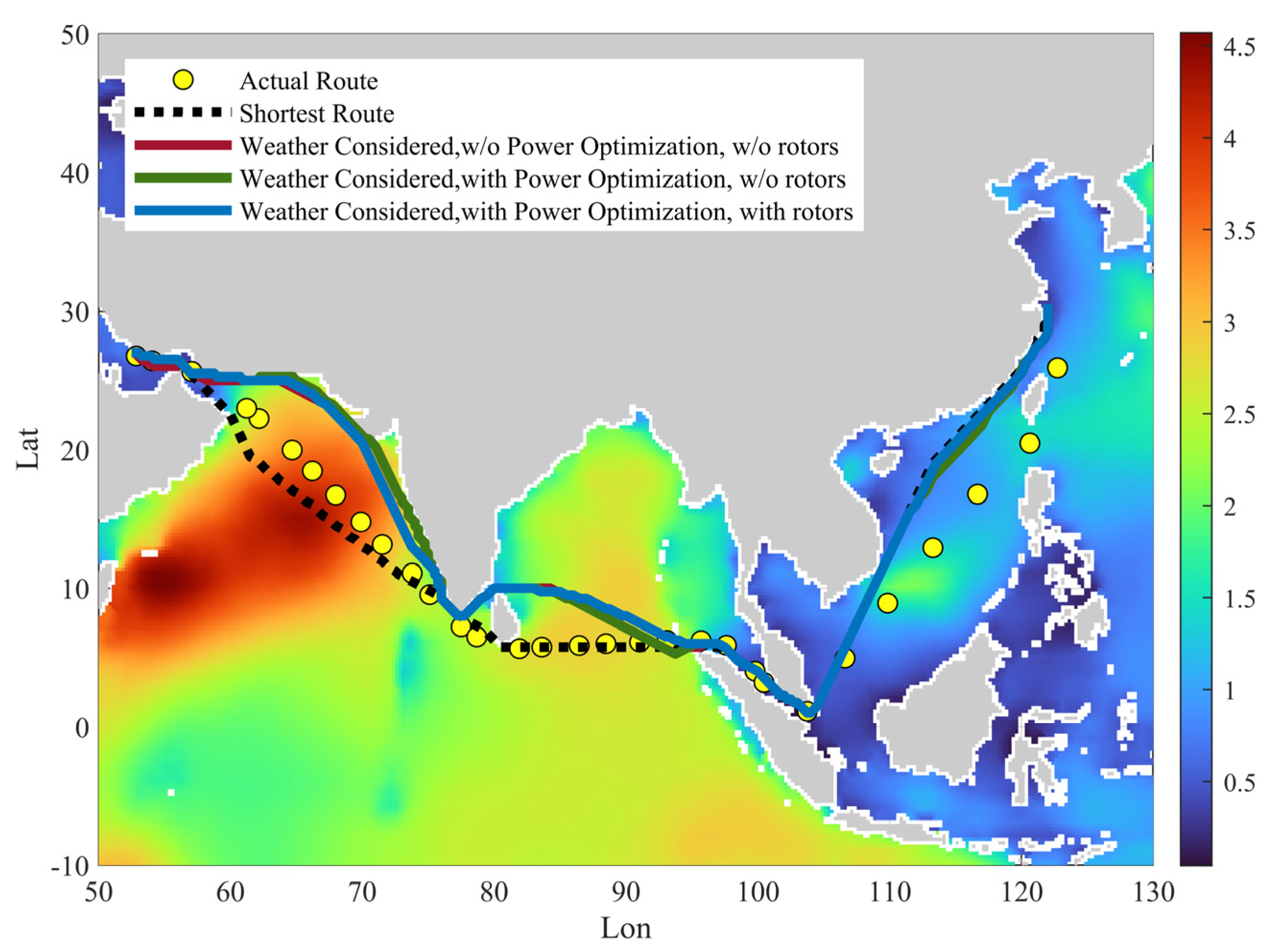
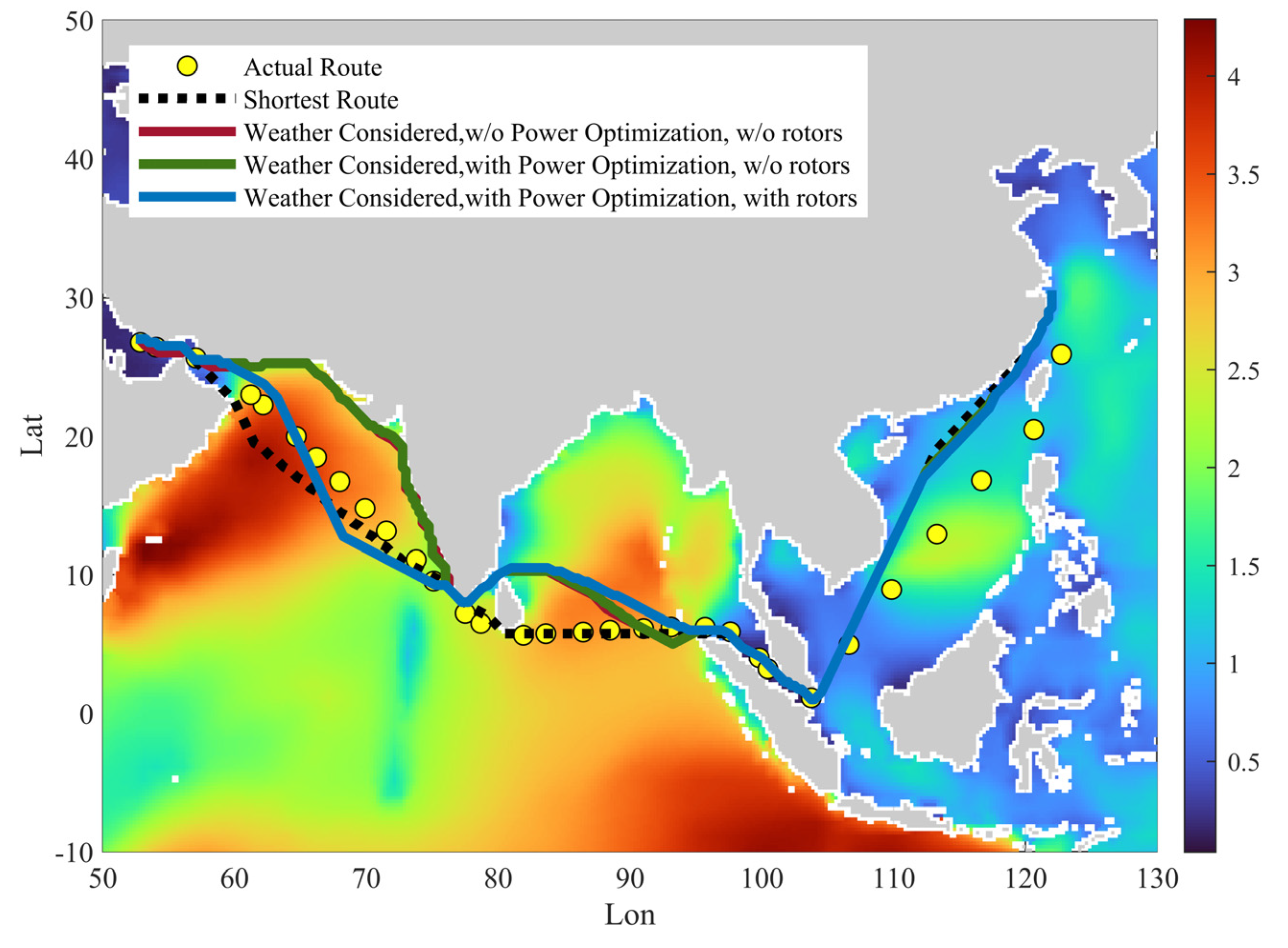
Four typical cases (1, 4, 6, 8) are selected to illustrate the difference of the resultant routes in geographic maps (Figure 18, Figure 19, Figure 20 and Figure 21). Considering the effect of s realistic ocean weather, the optimized routes will differ greatly from the simple shortest route especially for routes with speed optimization and rotors. The routes from weather routing could automatedly avoid severe sea conditions to achieve lower fuel consumption. For relatively mild sea states, like case 1 (Figure 18), the results from three different weather-routing strategies (MC2, MC3 and MC4) show similar routes. Usually, ships with wind-assisted rotors prefer to pass through some slightly rough seas to achieve a more beneficial side-wind for larger thrust from rotors (as shown in Figure 19 and Figure 21). When it meets a wide range of high ocean waves, the proposed method could plan routes to avoid additional fuel consumption.

4. Conclusions

An efficient and improved weather routing framework towards low-carbon shipping and CII reduction was proposed based on ocean weather forecast information and ship information considering the effect of an innovative energy-saving device: the wind-assisted rotor.

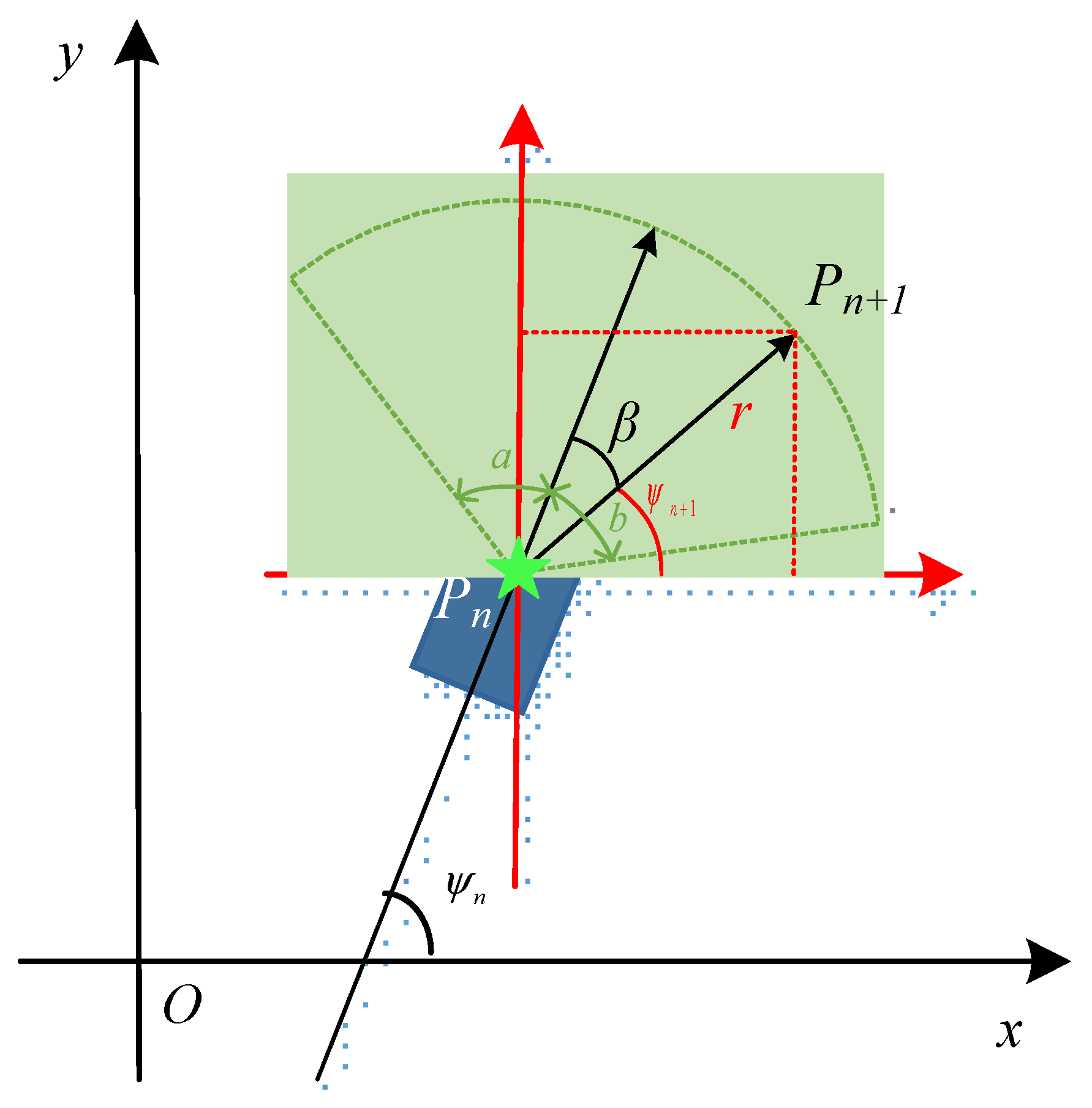
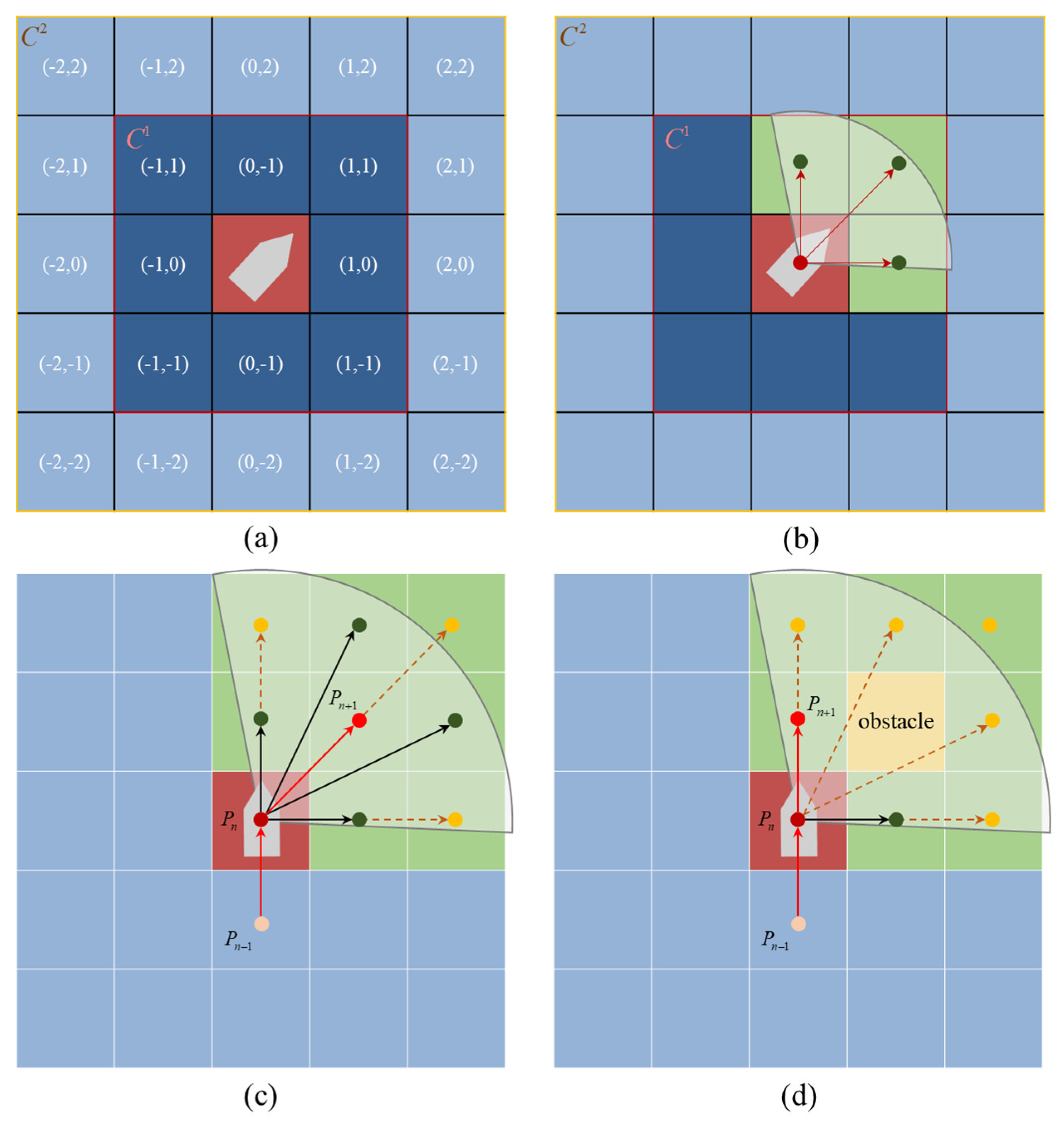
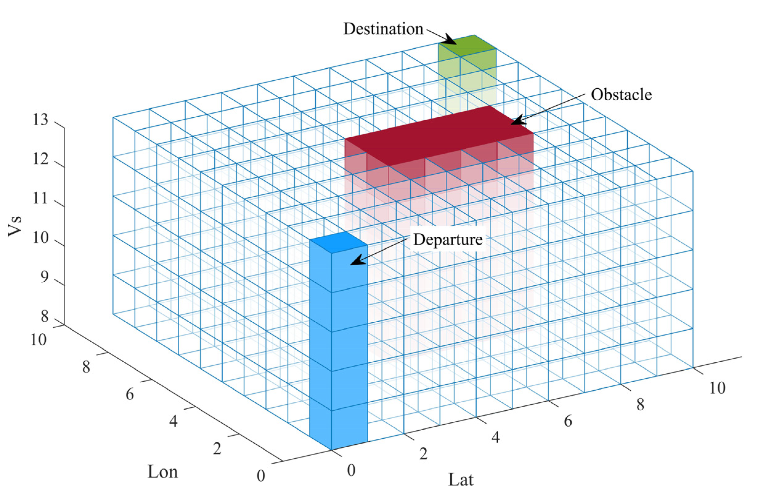
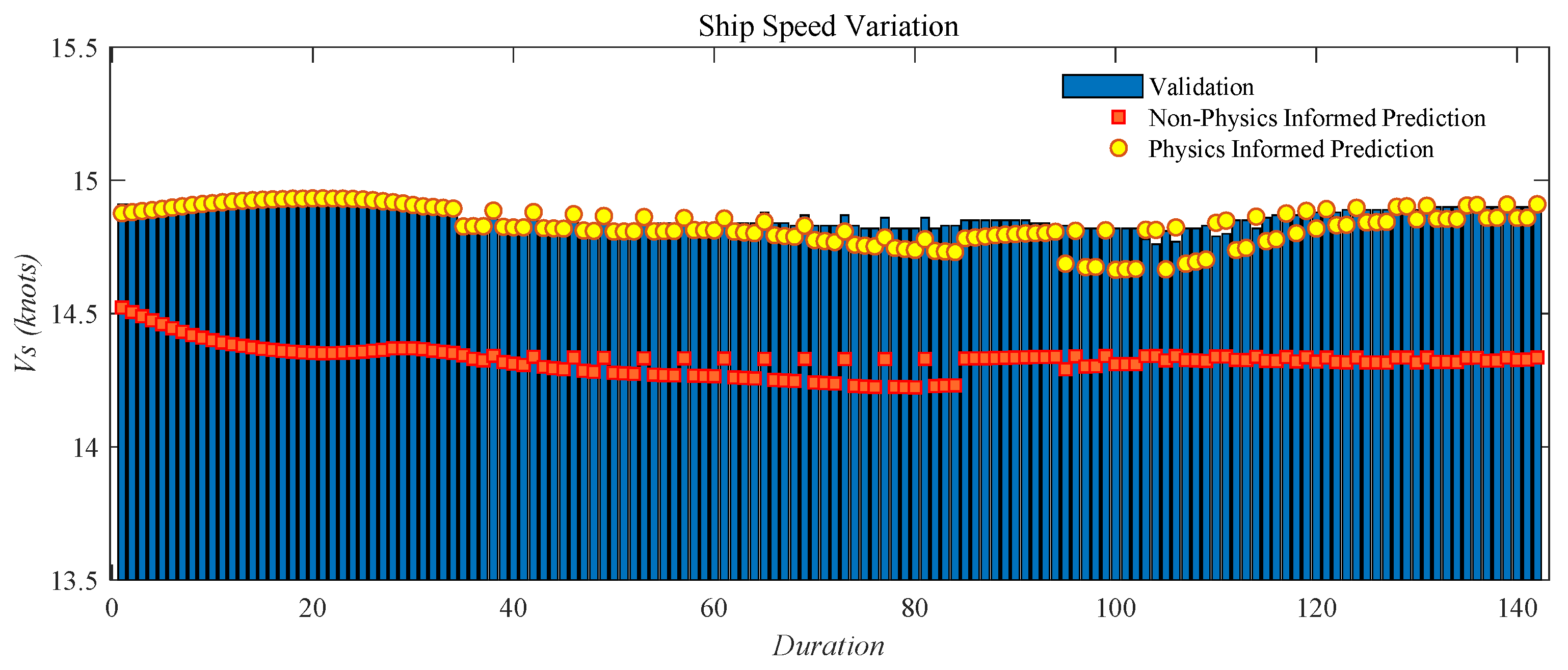
An improved A* algorithm including directed route searching and 3D capacity was presented in this paper with an enhancement of the searching range, searching efficiency and good incorporation with the operation optimization such as engine power and rotor speed. Additionally, based on historical ship report data, towering tank results and high-fidelity theory-based method for wave-added resistance and the air dynamic of wind-assisted rotors, a data-driven model for fast prediction of total fuel consumption was proposed and validated which could effectively replace the real-time calculation of the ship’s performance in a real sea state. The attained CII could be estimated, along with the routing task, to help monitor the carbon intensity of the current ship state.

The results show that the proposed method could generate optimized ship routes according to the local sea environment and the response of the ship. Compared to the shortest route, different combinations of routing methods could achieve the optimized route considering sea states that result in a reduction in TFOC, according to the sailing simulation for different cases. Statistically, weather routing, speed optimization and wind-assisted rotors could produce a 4.61%, 10.61% and 4.41% reduction in the total fuel consumption, respectively, in a single route from China to the Middle East and a similar reduction in the attained CII. The result shows that commercial ships, especially with environmentally dependent energy-saving devices such as rotors, could benefit a lot from proper weather routing and operation optimization.

With a joint optimization of ship speed, a higher energy saving could be achieved by economically modifying the engine power. The wind-assisted rotors could significantly provide a positive thrust and amplify the effect of route and operation optimization. In the Indian Ocean, wind-assisted rotors could have significant energy-saving possibilities for voyages with strong side-wind. The result proved that, with the proposed method, a more adaptive and economic solution for ship operation could be obtained, especially for ships with wind-assisted rotors.

In this paper, we proposed a general framework including the optimization method, TFOC estimation and route-generation procedure for economic ship routing and ship operation. It needs to be acknowledged that the analysis and simulations performed in this paper provide an ideal environment for the ship’s operation. It ignored the conditions when desired operations, such as the speed governing of the main engine and the driving motors of rotors, could not be achieved ideally. Additionally, the effect of wind-assisted rotors could be affected by the local properties of winds, waves, the ship’s motion and rudders. In the future, with more widespread applications of this kind of energy-saving device and more actual sailing data, the estimation could be more accurate for better routing.

In the future, more realistic models for the estimation of TFOC and safety should be considered to improve the engineering applicability of the current method. Additional objective functions should be tested in the economic ship-routing practice and the method should serve as state-of-the-art software for ships in operation. More detailed information from electronic sea charts and weather forecasts should be considered and more realistic demands from ship captains should be fully considered.

References

1. IMO. Resolution MEPC.352(78)—2022 Guidelines on Operational Carbon Intensity Indicators and the Calculation Methods (CII Guidelines, G1); IMO: London, UK, 2022. [Google Scholar]
2. IMO. Resolution MEPC.308(73)—2018 Guidelines on the Method of Calculation of the Attained Energy Efficiency Design Index (EEDI) for New Ships; IMO: London, UK, 2018. [Google Scholar]
3. IMO. Resolution MEPC.353(78)—2022 Guidelines on the Reference Lines for Use with Operational Carbon Intensity Indicators (CII Reference Lines Guidelines, G2); IMO: London, UK, 2022. [Google Scholar]
4. IMO. Resolution MEPC.338(76)—2021 Guidelines on the Operational Carbon Intensity Reduction Factors Relative to Reference Lines (CII Reduction Factors Guidelines, G3); IMO: London, UK, 2021. [Google Scholar]
5. Perera, L.P.; Soares, C.G. Collision risk detection and quantification in ship navigation with integrated bridge systems. Ocean Eng. 2015, 109, 344–354. [Google Scholar] [CrossRef]
6. Lee, S.M.; Roh, M.I. Method for a simultaneous determination of the path and the speed for ship route planning problems. Ocean Eng. 2018, 157, 301–312. [Google Scholar] [CrossRef]
7. Park, J.; Kim, N. Two-phase approach to optimal weather routing using geometric programming. J. Mar. Sci. Technol. 2015, 20, 679–688. [Google Scholar] [CrossRef]
8. Roh, M.I. Determination of an economical shipping route considering the effects of sea state for lower fuel consumption. Int. J. Nav. Archit. Ocean Eng. 2013, 5, 246–262. [Google Scholar] [CrossRef] [Green Version]
9. Wang, H.; Mao, W. A Three-Dimensional Dijkstra’s algorithm for multi-objective ship voyage optimization. Ocean Eng. 2019, 186, 106131. [Google Scholar] [CrossRef]
10. Gkerekos, C.; Lazakis, I. A novel, data-driven heuristic framework for vessel weather routing. Ocean Eng. 2020, 197, 106887. [Google Scholar] [CrossRef]
11. Hanssen, G.L.; James, R.W. Optimum ship routing. J. Navig. 1960, 13, 253–272. [Google Scholar] [CrossRef]
12. Ma, D.; Ma, W. Method for simultaneously optimizing ship route and speed with emission control areas. Ocean Eng. 2020, 202, 107170. [Google Scholar] [CrossRef]
13. Grifoll, M.; Borén, C. A comprehensive ship weather routing system using CMEMS products and A* algorithm. Ocean Eng. 2022, 255, 111427. [Google Scholar] [CrossRef]
14. Zaccone, R.; Figari, M. Energy efficient ship voyage planning by 3d dynamic programming. J. Ocean Technol. 2017, 12, 49–71. [Google Scholar]
15. Li, M.; Wang, S. Multi-Variable-Multi-Objective Optimization of Ship Routes under Rough Weather Condition. J. Navig. China 2020, 43, 14–19. [Google Scholar]
16. Zhang, G.; Wang, H. Application of improved multi-objective ant colony optimization algorithm in ship weather routing. J. Ocean Univ. China 2021, 20, 45–55. [Google Scholar] [CrossRef]
17. Du, W.; Li, Y. Ship weather routing optimization based on improved fractional order particle swarm optimization. Ocean Eng. 2022, 248, 110680. [Google Scholar] [CrossRef]
18. Hermans, A.J. Added Resistance by Means of Time-Domain Models in Seakeeping. J. Ship Res. 2005, 49, 252–262. [Google Scholar] [CrossRef]
19. Liu, S.; Papanikolaou, A. Prediction of added resistance of ships in waves. Ocean Eng. 2011, 38, 641–650. [Google Scholar] [CrossRef]
20. Hu, J.-P.; Wang, Y.-X. The dynamic Performance of a Rotating Frustum of a cone. In Proceedings of the Sixth International Symposium on Marin Propulsors, Rome, Italy, 26–30 May 2019. [Google Scholar]
21. ISO/DIS 15016; Guidelines for the Assessment of Speed and Power Performance by Analysis of Speed Trial Data. ISO: Geneva, Switzerland, 2002; pp. 1–45.
22. Gkerekos, C.; Lazakis, I. Machine learning models for predicting ship main engine Fuel Oil Consumption: A comparative study. Ocean Eng. 2019, 188, 106282. [Google Scholar] [CrossRef]
23. Zhang, C.; Zhang, D. Data-driven ship energy efficiency analysis and optimization model for route planning in ice-covered Arctic waters. Ocean Eng. 2019, 186, 106071. [Google Scholar] [CrossRef]
24. Wang, K.; Xu, H. Analysis of intelligent prediction method of ship energy consumption based on machine learning. Ship Eng. 2020, 42, 87–93. [Google Scholar]
25. Yin, Z.; Xu, J. Ship oil consumption optimization based on sailing data. Ship Eng. 2019, 41, 100–104. [Google Scholar]
26. Farag, Y.B.A.; Ölçer, A.I. The development of a ship performance model in varying operating conditions based on ANN and regression techniques. Ocean Eng. 2020, 198, 106972. [Google Scholar] [CrossRef]
27. Wang, S.; Ji, B. Predicting ship fuel consumption based on LASSO regression. Transp. Res. Part D Transp. Environ. 2018, 65, 17–824. [Google Scholar] [CrossRef]
28. Wei, J.-F.; Chen, J.-P. The study on the calculation method of ship speed loss coefficient (fw) considering added resistance in short waves. Chin. J. Hydrodyn. 2013, 28, 144–150. [Google Scholar]
Figure 1. Scheme of the proposed weather-routing framework.
Jmse 10 01979 g001
Figure 2. Ship’s speed/power trail performance (left) and main engine’s SFOC curve (right).
Jmse 10 01979 g002
Figure 3. Propeller’s open water performance (left) and rotor’s air dynamic performance (right).
Jmse 10 01979 g003
Figure 4. Discretization of geographic information.
Jmse 10 01979 g004
Figure 5. Geographic map and its computational grid for weather routing.
Jmse 10 01979 g005
Figure 6. Significant wave height interpolated to computational grid worldwide.
Jmse 10 01979 g006
Figure 7. Significant wave height and wind field of north Pacific Ocean for three continuous days.
Jmse 10 01979 g007
Figure 8. Noon report data of a VLCC’s voyage in 2019.
Jmse 10 01979 g008
Figure 9. Relationship of main engine rpm with power and FOC.
Jmse 10 01979 g009
Figure 10. Variable searching region depending on the current ship status.
Jmse 10 01979 g010
Figure 11. Illustration of the calculation of searching region. (a) Representation of navigable area; (b) Route searching region; (c) Available nodes without obstacle; (d) Available nodes with obstacle.
Jmse 10 01979 g011
Figure 12. Three-dimensional A* algorithm for speed optimization.
Jmse 10 01979 g012
Figure 13. Illustration of optimal path searching result in 3D (left) and 2D projection (right).
Jmse 10 01979 g013
Figure 14. Mechanism of wind-assisted rotors.
Jmse 10 01979 g014
Figure 15. Maximum thrust at different relative wind angle with corresponding optimal spinning ratio.
Jmse 10 01979 g015
Figure 16. Validation of ANN prediction of resultant ship speed.
Jmse 10 01979 g016
Figure 17. Results of TFOC, voyage time and the attained CII for different cases.
Jmse 10 01979 g017
Figure 18. Result for ship weather routing for Case 1.
Jmse 10 01979 g018
Figure 19. Result for ship weather routing for Case 4.
Jmse 10 01979 g019
Figure 20. Result for ship weather routing for Case 6.
Jmse 10 01979 g020
Figure 21. Result for ship weather routing for Case 8.
Jmse 10 01979 g021