Wave Motion and Seabed Response around a Vertical Structure Sheltered by Submerged Breakwaters with Fabry–Pérot Resonance

Abstract

This paper presents the results from a numerical simulation study to investigate wave trapping by a series of trapezoidal porous submerged breakwaters near a vertical breakwater, as well as the seabed response around the vertical breakwater. An integrated model, based on the volume-averaged Reynolds-averaged Navier–Stokes (VARANS) equations is developed to simulate the flow field, while the dynamic Biot’s equations are used for simulating the wave-induced seabed response. The reflection of the wave energy over the submerged breakwaters, caused by the vertical breakwater, can be reserved, indicating that the existence of the submerged breakwaters in the front of the vertical breakwater can either provide shelter or worsen the hazards to the vertical breakwater. Numerical examples show two different modes under the Fabry–Pérot (F–P) resonance condition of the wave transformation, namely the wave reflection (Mode 1) and the wave trapping (Mode 2). The distance between the submerged breakwaters and the vertical breakwater, is a key parameter dominating the local hydrodynamic process and the resultant dynamic stresses around the vertical breakwater. The numerical results indicated that more submerged breakwaters and a higher porosity of submerged breakwaters will obviously dissipate more wave energy, and hence induce a smaller wave force on the rear vertical breakwater and liquefaction area around the vertical breakwater.

1. Introduction

Breakwaters are commonly used to shelter the coastlines or harbors, by dissipating and reflecting the incoming waves. Meanwhile, the existence of breakwaters may significantly affect the wave motion and its associated seabed response around the structures. Nowadays, permeable or impermeable submerged breakwaters are usually constructed in front of a seawall or caisson breakwater, to reduce the wave forces acting on the vertical wall [1]. Because of the lower crown, the submerged breakwaters have the advantages of low construction costs, early wave breaking, and the effective reduction of the wave height on the lee side, and they do not obstruct the sea-view.

Water waves propagating from offshore to near-shore zones may experience various transformations, such as diffraction, refraction, reflection, and shoaling, induced by the variation of the bottom topography or the interaction with structures [2]. The reflection by the multiple bars can be amplified when the surface wavelength is two times larger than that of the sand bar wavelength, which is called the Bragg resonance [3,4,5]. From the point of view of engineering practices [6], the wave reflection by the sand bars has been considered as a good measure to protect the shoreline and coastal structures. Extensive studies have been conducted to extend this concept to multiple submerged breakwaters [7,8,9,10,11,12,13]. A common subject discussed in those studies, is on the scattering of waves by multi-arrayed submerged breakwaters in an open channel, and the outgoing wave energy is assumed to be dissipated, completely.

In the field, there is always some reflection from rear structures, owing to the incomplete dissipation by the breaking or frictional effect. With the reflected wave from the rear side re-entering the submerged breakwaters’ field, the wave transformation becomes more complicated. A numerical simulation [14] and analytical analysis [15,16] were conducted to examine the effect of the partial reflection, from the rear side on the Bragg resonance. In these studies, the wave field was assumed to be the inviscid and irrotational fluid, transforming across the impermeable periodic structure. The frontal submerged breakwaters and the rear reflector work as two reflective mirrors in the Fabry–Pérot (F–P) cavities, which are widely used in optics, quantum physics, and astronomy. Waves entering the cavity undergo multiple reflections between the submerged breakwaters. Unlike the traditional F–P cavities used in optics without considering the dissipation, the incoming water wave energy is decomposed into three parts, while the partial energy is reflected back and the rest is dissipated or trapped between structures. Based on the long wave theory and energy dissipation of the permeable structures, Terrett et al. [17] and Chwang [18] investigated the wave trapping by a porous wall with a solid backwall. They concluded that the reflection coefficient reached its lowest value when the distance $S,$ between the porous plate and a vertical wall, was equal to an integer multiple of the quarter of the wave length L, namely,$S/L=n/4;n=1,3,5,\dots$, and the porous structure lost its wave damping efficiency for $n=2,4,6,\dots$ Recently, Behera and Khan [6] used a multi-domain boundary element method to investigate the wave energy attenuation caused by the double trapezoidal porous structures near a porous wall. Their results indicated that the double trapezoidal structures in the presence of the porous seawall were the effective configuration, in terms of reducing the wave force acting on the vertical wall. However, their investigation was under the assumption of the linear wave theory, and completely ignored the nonlinear wave-wave interaction. Unlike the study on the existence of the trapped mode, discussed in the aforementioned studies, the emphasis of this study is to analyze the effect of the F–P resonance on the wave transformation and trapping, and to evaluate the stability of the rear structure and seabed around the coastal structures.

There have been extensive experimental and numerical studies on the wave-induced seabed response around marine structures [19,20,21,22,23]. By applying a boundary element method (BEM) and a finite element method (FEM) model, Mizutani and Mostafa [24] investigated the nonlinear wave-induced seabed instability around coastal structures. Hur et al. [25] studied the flow characteristics in the permeable structure and the sandy seabed. They found that the flow within the seabed was dominated by the laminar flow effect. Based on the assumption of the negligible effect of the poro-elastic deformations on the wave transformation, Zhang et al. [26] developed a one-way coupling model, combining the volume-averaged Reynolds-averaged Navier–Stokes (VARANS) equations for the wave field and Biot’s consolidation equations for the seabed. Their results indicated that the seabed response around the permeable submerged breakwaters was highly dependent on the process of the wave propagation and soil characteristics. The one-way coupling model is further enhanced to include the inertial forces associated with the soil skeleton by the “$u_s-p_s$” ($u_s$ is soil displacement; $p_s$ is pore pressure) approximation [13], to describe the wave motion and its induced seabed response. It turned out that the wave amplitude largely decreased at the back side of the structures, owing to the Bragg reflection. However, all of these previous studies have only focused on the multiple permeable structures in an open channel. A study on the seabed response beneath multiple permeable submerged breakwaters in a closed-end channel, is still not available.

Recently, a series of submerged breakwaters have been used to shelter the rear structure on the Hainan coast, in China. To ensure the sufficient water area, the rear structure adopted the vertical form, which was expected to effectively reflect the wave back to the frontal submerged breakwaters. For such kinds of breakwater arrangements, however, it is not clear how the F–P resonance affects the wave transformation and trapping, and thus the stability of the rear vertical structure. This motivates this study. The plan of this paper is as follows. The effectiveness of this one-way coupling method will be discussed in Section 2. The mathematical formulations and the POROus model for the wave-seabed-structure interaction version II (PORO-WSSI II), are also briefly presented in Section 2, in which the VARANS equations are used for the wave sub-model, and the dynamic Biot theory is then used for the porous seabed sub-model. The PORO-WSSI II model proposed by Zhang et al. [13] is further developed to include a wide range of porous flow from the laminar, transitional, and fully turbulent flows. The model validation is presented in Section 3 by using the laboratory experiments of Cho et al. [11] and Tsai and Lee [27]. The details of the wave trapping under the F–P resonance condition are given in Section 4, in which two modes about the wave transformation are defined. Meanwhile, the effects of the wave periods, and structure properties (number and porosity of the submerged breakwaters, the phase of the rear breakwater reflection, relative to that of the submerged breakwaters) on the wave transformation, and the stability of the rigid breakwater, are discussed. Finally, the conclusions are summarized in Section 5.

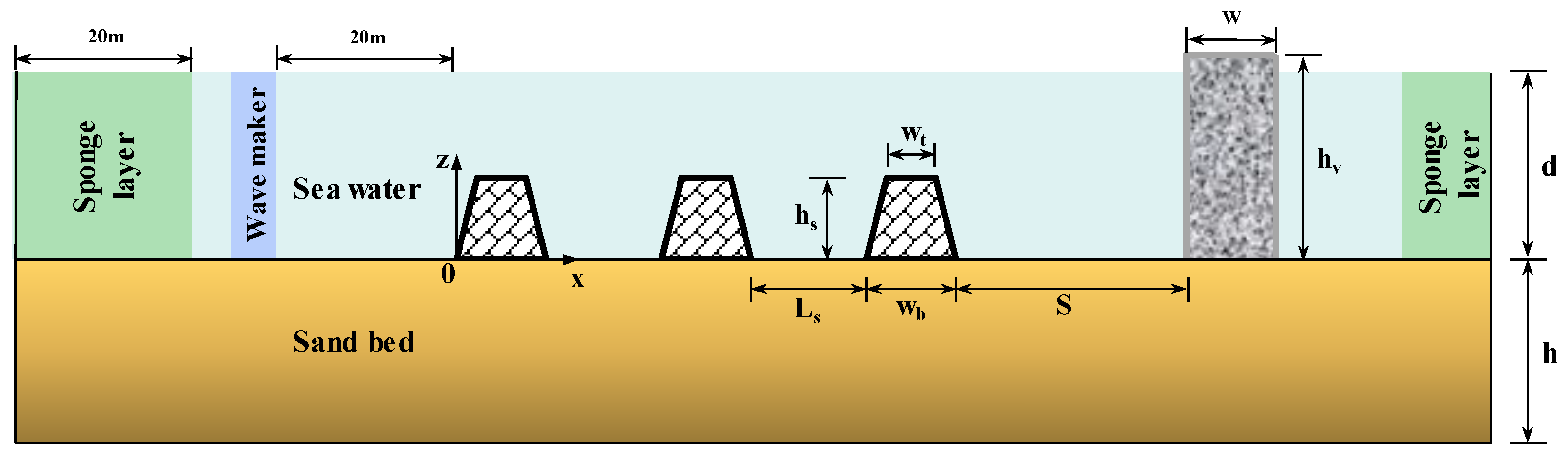
2. Numerical Model

In this study, the model PORO-WSSI II [13] is enhanced to simulate the wave-seabed-structure interaction. In this one-way coupling model, the small deformation and percolation in the seabed are assumed not to affect the wave transformation. Due to the dissipation of the wave energy, the Reynolds number (Re) of the flow inside the rear submerged breakwaters is much smaller than that in the frontal breakwater. In the study of Zhang et al. [13], the inner and outer flows of the porous breakwater are described by the VARANS equations, while the porous flow model only consider the resistance force in the laminar and fully turbulent flow regimes. Therefore, the main feature of the proposed model is the inclusion of a wider range of flow regimes. To account for the dynamic mechanical behaviors of the structures and the seabed, the dynamic Biot model is adopted. The pressure calculated from the VARANS model will be used as the seabed boundary condition in the dynamic Biot model.

It is well known that the wave transformation is highly dependent on the soil dynamic response to the wave loading. Unlike the viscous dissipation generated by the deformation of the silty seabed, the primary mechanism of the wave energy dissipation in the sandy seabed is the friction within the porous structure [28]. Therefore, it is reasonable to ignore the influence of the seabed deformation on the wave transformation. The details of this one-way integrating procedure can be found in Zhang et al. [26] and will not be repeated here.

2.1. Wave Sub-Model

For a turbulent flow, all of the flow variables represented by $\phi$ are decomposed into time average term $\overline{\phi }$ and the turbulent terms ${\phi }^{\prime }$ as well as into the ensemble-intrinsic volume average ${\langle \overline{\phi }\rangle }^f$. Thus, the turbulent flow field is governed by the following VARANS equations [29]:

$$\frac{\partial \langle \overline{u_i}\rangle }{\partial x_i}=0$$

(1)

$$\frac{1+C_A}{n}\frac{\langle \partial \overline{u_i}\rangle }{\partial t}+\frac{\langle \overline{u_j}\rangle }{n}\frac{\partial }{\partial x_j}\frac{\langle \overline{u_i}\rangle }{n}=-\frac{1}{{\rho }_f}\frac{\partial {\langle \overline{p}\rangle }^f}{\partial x_i}+\frac{1}{n{\rho }_f}\frac{\partial \langle \overline{{\tau }_{ij}}\rangle }{\partial x_j}-\frac{1}{n^2}\frac{\partial \langle \overline{u_i^{\prime }{u}_j^{\prime }}\rangle }{\partial x_j}-f_{Di}$$

(2)

where $u_i$ is the flow velocity (written as $u_i=\left(u,v\right)$ for simplicity); $x_i$ is the Cartesian coordinate; $t$ is the time, ${\rho }_f$ is the density of the fluid; $p$ is the pressure; ${\tau }_{ij}$ is the viscous stress tensor of the mean flow; $g_i$ is the $i$th component of the gravitational acceleration; $n$ is the porosity of the porous material; $c_A=0.34\left(\left(1-n\right)/n\right)$ denotes the added mass coefficient;$\langle \overline{u_i^{\prime }{u}_j^{\prime }}\rangle$ is Darcy’s volume averaged Reynolds stress that can be obtained by solving the modified $\kappa -\epsilon$ ($\kappa$ is the kinetic energy and $\epsilon$ is the dissipation rate of the kinetic energy) equations and the nonlinear eddy viscosity model [30]; “〈⬚〉” and “${\langle ⬚\rangle }^f$” stand for Darcy’s volume averaging operator and the intrinsic averaging operator.

In the VARANS model, the drag force $f_{Di}$ is resulted from the spatial perturbation of the velocity and pressure, which can be simulated as following [31]:

$$f_{Di}=\frac{3}{4}{C}_D\frac{1-n}{n^3}\frac{1}{d_{50}}{u}_c\langle \overline{u_i}\rangle$$

(3)

where $C_D$ is the drag force coefficient; $d_{50}$ is the equivalent mean diameter of the porous material, and the instantaneous horizontal wave orbital velocity $u_c$ can be estimated by $u_c=\sqrt{\langle \overline{u_i}\rangle \langle \overline{u_i}\rangle }$. It is obvious that in the free fluid region, i.e., $n=1$ and $c_A=f_{Di}=0$, the VARANS equations return to the original RANS equations. In this study, the empirical formula of the drag coefficient for a single smooth sphere $C_{Ds}$ given by Fair [32], is employed:

$$C_{Ds}=\frac{24}{\mathrm{Re}}+\frac{3}{\sqrt{\mathrm{Re}}}+0.34$$

(4)

where $\mathrm{Re}=\left|U\right|d_{50}/\upsilon$ with $U$ being a typical velocity scale and $\upsilon$ being the fluid viscosity.

In Equation (4), the first term means the conventional linear friction force for the flow with a small $\mathrm{Re}$, the other terms are the correction terms of the friction force for the transitional flow, and for the fully turbulent flow (large $\mathrm{Re}$), the nonlinear drag coefficient can be approximated as a constant $C_{Ds}=0.34$. To account for other effects, i.e., the influence of the pore shape, wetted surface, tortuosity factor, and path length [33], the final form of $C_D$ is corrected as [32]:

$$C_D=C_1\frac{24}{\mathrm{Re}}+\left(C_2\frac{3}{\sqrt{\mathrm{Re}}}+0.34C_3\right)\left(1+\frac{7.5}{\mathrm{KC}}\right)$$

(5)

where $\mathrm{KC}=u_{c}T/\left(n{d}_{50}\right)$. To obtain the values of the empirical coefficients $C_1$, $C_2,$ and $C_3$, we consider a one dimensional (1D) steady flow in sand, described as the following:

$$-\frac{1}{{\rho }_f}\frac{\partial p}{\partial x}=AU+B\sqrt{\left|U\right|}U+C\left|U\right|U$$

(6)

where

$$A=18C_1\frac{1-n}{n^3}\frac{\upsilon }{d_{50}^2}; B=2.25C_2\frac{1-n}{n^3}\frac{{\upsilon }^{1/2}}{d_{50}^{3/2}};\mathrm{and}C=0.255C_3\frac{1-n}{n^3}\frac{1}{d_{50}}$$

(7)

It is interesting to find that if the empirical coefficients $C_1=\frac{100}{9}\left(1-n\right)$, $C_2=0,$ and $C_3=4.3$ are adopted, Equation (6) shows the same expression with the model, proposed by Liu et al. [34]. Considering the transitional term, the modified values of $C_1=5$ and $C_3=2$ are used in this study. The range of $C_2,$ suggested by Lin and Karunarathna [35], is from 1.8 to 4.2. Therefore, $C_2=2$ is adopted in this study.

2.2. Seabed Sub-Model

In this study, an unsaturated porous seabed is assumed to be hydraulically isotropic (with the same permeability $K$ in all directions), and the flow inside the seabed obeys Darcy’s law. As such, the dynamic Biot equations (the so-called “$u_s-p_s$” approximation, $u_s$ is the soil displacement in the horizontal direction; $p_s$ is the pore pressure) proposed by Zienkiewicz et al. [36], are used to describe the dynamic seabed response around the structures. The acceleration, due to the soil motion, is considered in the present seabed sub-model, while the relative acceleration, due to the pore fluid, is ignored. The governing equations are:

$${\nabla }^2{p}_s-\frac{{\gamma }_w{n}_s{\beta }_s}{K}\frac{\partial p_s}{\partial t}+{\rho }_f\frac{{\partial }^2{\epsilon }_s}{\partial t^2}=\frac{{\gamma }_w}{K}\frac{\partial {\epsilon }_s}{\partial t}$$

(8)

$$\frac{\partial {\sigma }_x^{\prime }}{\partial x}+\frac{\partial {\tau }_{xz}}{\partial z}=\frac{\partial p_s}{\partial x}+\rho \frac{{\partial }^2{u}_s}{\partial t^2}$$

(9)

$$\frac{\partial {\tau }_{zx}}{\partial x}+\frac{\partial {\sigma }_z^{\prime }}{\partial z}+\rho g=\frac{\partial p_s}{\partial z}+\rho \frac{{\partial }^2{w}_s}{\partial t^2}$$

(10)

where $w_s$ is the soil displacement in the vertical direction; $p_s$ is the pore pressure; ${\gamma }_w$ is the unit weight of the pore water; $n_s$ is the soil porosity; ${\sigma }_x^{\prime }$ and ${\sigma }_z^{\prime }$ are the effective normal stresses in the horizontal and vertical directions, respectively; ${\tau }_{xz}$ is the shear stress; $\rho ={\rho }_f{n}_s+{\rho }_s\left(1-n_s\right)$ is the average density of the porous seabed; ${\rho }_s$ is the soil density; $K$ is Darcy’s permeability; ${\epsilon }_s$ is the volume strain; and ${\beta }_s$ is the compressibility of the pore fluid; defined as:

$${\epsilon }_s=\frac{\partial u_s}{\partial x}+\frac{\partial w_s}{\partial z} \mathrm{and}{\beta }_s=\frac{1}{K_w}+\frac{1-S_r}{P_{w0}}$$

(11)

where $K_w$ is the bulk modulus of the pore water (taken as $2\times {10}^9\mathrm{N}/{\mathrm{m}}^2$); $S_r$ indicates the saturated degree of the seabed; $P_{w0}$ is the absolute water pressure.

The effective stress and strain of the solid matrix are determined by Hooke’s law:

$${\sigma }_x^{\prime }=2G\left[\frac{\partial u_s}{\partial x}+\frac{{\mu }_s}{1-2{\mu }_s}{\epsilon }_s\right]$$

(12)

$${\sigma }_z^{\prime }=2G\left[\frac{\partial w_s}{\partial z}+\frac{{\mu }_s}{1-2{\mu }_s}{\epsilon }_s\right]$$

(13)

$${\tau }_{xz}={\tau }_{zx}=G\left[\frac{\partial u_s}{\partial z}+\frac{\partial w_s}{\partial x}\right]$$

(14)

where $G$ is the shear modulus; and ${\mu }_s$ is Poisson’s ratio. The shear modulus $G$ of the soil generally varies with the static normal effective stress in the sandy seabed [37]:

$$G=C_g{p}_a\frac{{\left(e_r-e\right)}^2}{1+e}{\left(\frac{{\sigma }_0}{p_a}\right)}^{n_g}$$

(15)

where, $C_g$ and $n_g$ are nondimensional soil parameters and are respectively taken as 612 and 0.439 for the sand [38]; $p_a$ is the air pressure; $e_r=2.17$ for the sand particles ranging from round to angular in shape [37]; $e$ is the void ratio of the sandy soil; and ${\sigma }_0$ is the initial mean normal effective stress, defined as:

$${\sigma }_0=\frac{{\sigma }_1+2{\sigma }_3}{3}$$

(16)

in which ${\sigma }_1$ and ${\sigma }_3$ are the maximum and the minimum principal effective stresses, respectively. In this study, the seabed sub-model is solved by the finite-element method.

2.3. Boundary Conditions

Appropriate boundary conditions are required to solve the governing equations. In the wave sub-model, the two-phase volume of fluid (VOF) method [39] is used to track the water-air interface and the zero-stress condition is adopted on the mean free surface by neglecting the effect of the air flow (${\tau }_{ij}=0$). On the seabed surface, a no-slip boundary condition is imposed for the mean flow field ($u_i=0$). For the turbulence field, the log-law distribution of the mean tangential velocity in the turbulent boundary layer is applied in the grid point immediately above the sea floor. The zero-gradient boundary conditions are also imposed for both the turbulent kinetic energy $\kappa$ and its dissipation rate $\epsilon$ on the free surface (i.e., $\partial \kappa /\partial \overrightarrow{n}=\partial \epsilon /\partial \overrightarrow{n}=0$). To run for a sufficiently long time until the waves reach the quasi-steady state, a combination of the numerical sponge layers and the radiation boundaries are used at the two lateral sides.

In the geotechnical module, on the seabed surface, it is assumed that the vertical effective normal stress ${\sigma }_z^{\prime }$ and the shear stress ${\tau }_{xz}$ are negligible, compared to the large amplitude wave pressure in this study, while the pore pressure $p_s$ is equal to the dynamic wave pressure $p_d,$ calculated from the VARANS model:

$$p_s=p_d, \mathrm{and}{\sigma }_z^{\prime }={\tau }_{xz}=0 \mathrm{at}z=0$$

(17)

The bottom of the seabed is considered to be impermeable and rigid, while the soil displacement and the normal gradient pore pressure are specified as zero:

$$\frac{\partial p_s}{\partial z}=0, \mathrm{and}{u}_s=w_s=0 \mathrm{at}z=-H_s$$

(18)

The structure can move freely, whereas the pressure imposed by the wave impact is applied perpendicularly to the outer surface of the structure. At the soil-structure interface, a no-slip condition for the soil displacement is imposed.

2.4. Numerical Scheme

In the numerical model, the same discretization of the uniform $\Delta x=0.01 \mathrm{m}$ and $\Delta z=0.005 \mathrm{m},$ is used for both validations and the present simulations in the wave sub-mode. In the soil model, the optimal triangular FEM meshes were generated by the COMSOL software with a maximum element size scaling factor 0.02, to control the maximum allowed element size, in this study. Both the Courant-Friedrichs-Lewy condition, (19) and the diffusive limit condition, (20) were adopted to obtain the automatically adjustable time interval, to obtain the computational stability.

$$\Delta t\le {\alpha }_1\underset{}{\min }\left(\frac{\Delta x}{{\left|u\right|}_{\max }},\frac{\Delta z}{{\left|v\right|}_{\max }}\right)$$

(19)

$$\Delta t\le {\alpha }_2\frac{1}{2\left(\upsilon +{\upsilon }_t\right)}{\left[\frac{1}{1/{\left(\Delta x\right)}^2+1/{\left(\Delta z\right)}^2}\right]}^{1/2}$$

(20)

where ${\left|u\right|}_{\max }$ and ${\left|v\right|}_{\max }$ are the maximum flow velocities, and the empirical coefficients are ${\alpha }_1=\frac{3}{10}$ and ${\alpha }_2=\frac{2}{3}$, in this study.

3. Model Validation

To validate the proposed numerical model, two available laboratory experiments, conducted by Cho et al. [11] and Tsai and Lee [27], are used. The configurations of the laboratory experiments are shown in Figure 1, Figure 2 and Figure 3, respectively.

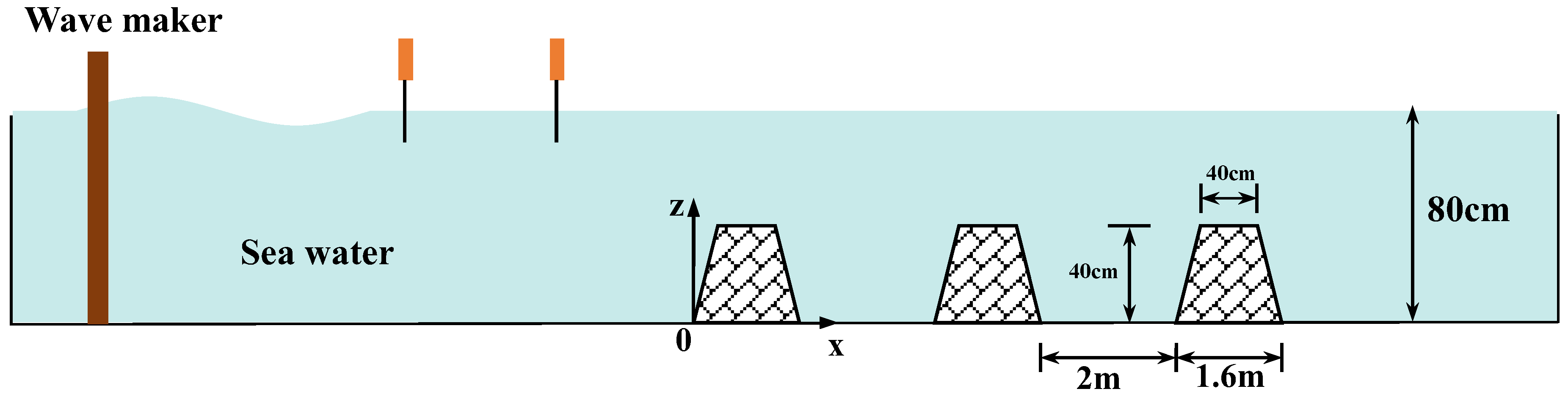
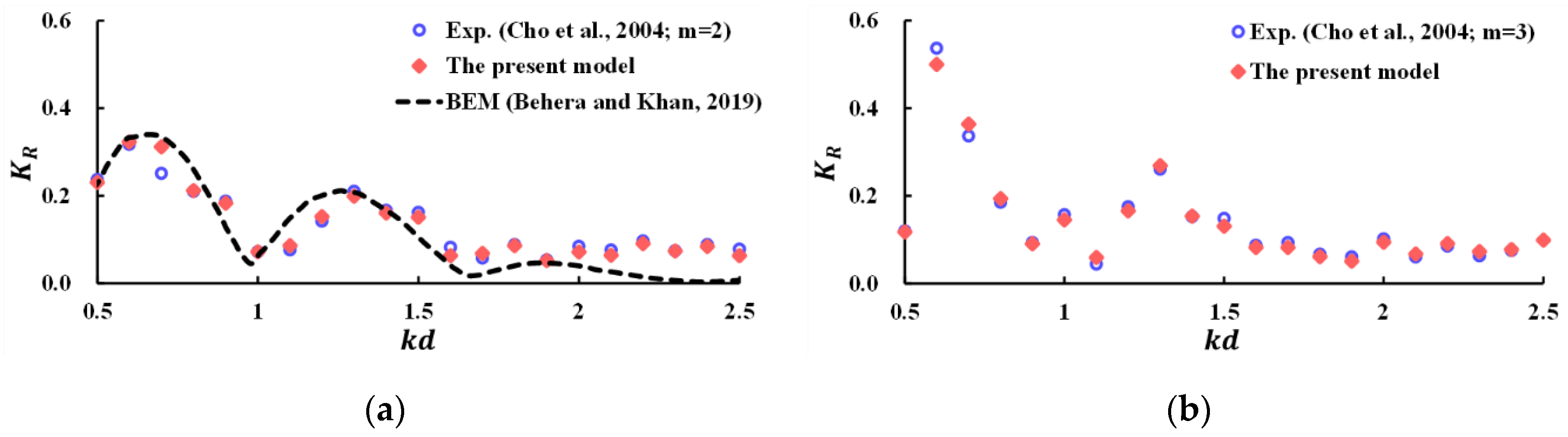
3.1. Validation for the Wave Reflection

The results evaluated for the reflection coefficient ($K_R$) in the present study, using the VOF numerical scheme, are compared with the experimental measurements by Cho et al. [11]. In the laboratory experiments, the periods of incident waves were 1.14~3.73 s and the incident wave height was 0.04 m. The numerical boundary element method (BEM) results with an assumption of the linear wave theory, by Behera and Khan [6], who investigated the wave attenuation, due to the multi-arrayed trapezoidal submerged breakwaters, are also used for comparison. In this example, the reflection coefficients are determined by the measurements of the two wave gauges, installed in front of the submerged breakwaters. The separation of the incident and the reflected waves are carried out by the method of Goda and Suzuki [40]. Figure 2 shows the comparison of the simulated and measured reflection coefficient $K_R$ for the different breakwater numbers. There are some discrepancies between the experimental and the BEM of Behera and Khan [6], especially when the period of the incident wave is short (e.g., $kd>1.5$; where k is the wave number and d is the still water depth). It is seen that, with the consideration of the non-linear effect, the reflection coefficient predicted in this study generally agrees well with the measurements.

Figure 2 shows that the reflection coefficient is highly dependent on the wave period and has an oscillation variation with kd. For $m=2$ ($m$ denotes the number of the submerged breakwater), the reflection coefficient reaches a maximum $K_R=0.32$ at $kd=0.6$ and a second peak $K_R=0.20,$ corresponding to the sub-resonance occurring at $kd=1.3$. At $kd=1.0,$ the submerged breakwaters have little effect on the reflection. The reflection coefficient of the three arrays ($m=3$) shows a similar resonance period but the magnitude of the reflection coefficient is larger than those for two breakwaters $(e.g.K_R=0.50$ at $kd=0.6)$. The small wave energy is reflected back at $kd=1.1$ for m=3. When the period of the incident wave is short $\left(kd>1.5\right)$, the non-linearity is more important than the Bragg resonance [12].

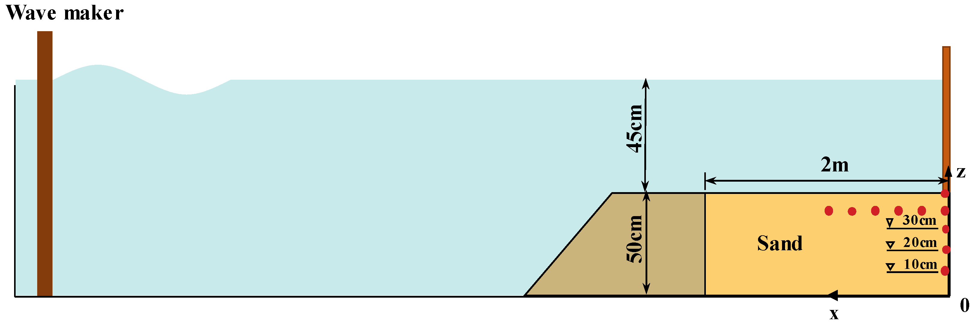
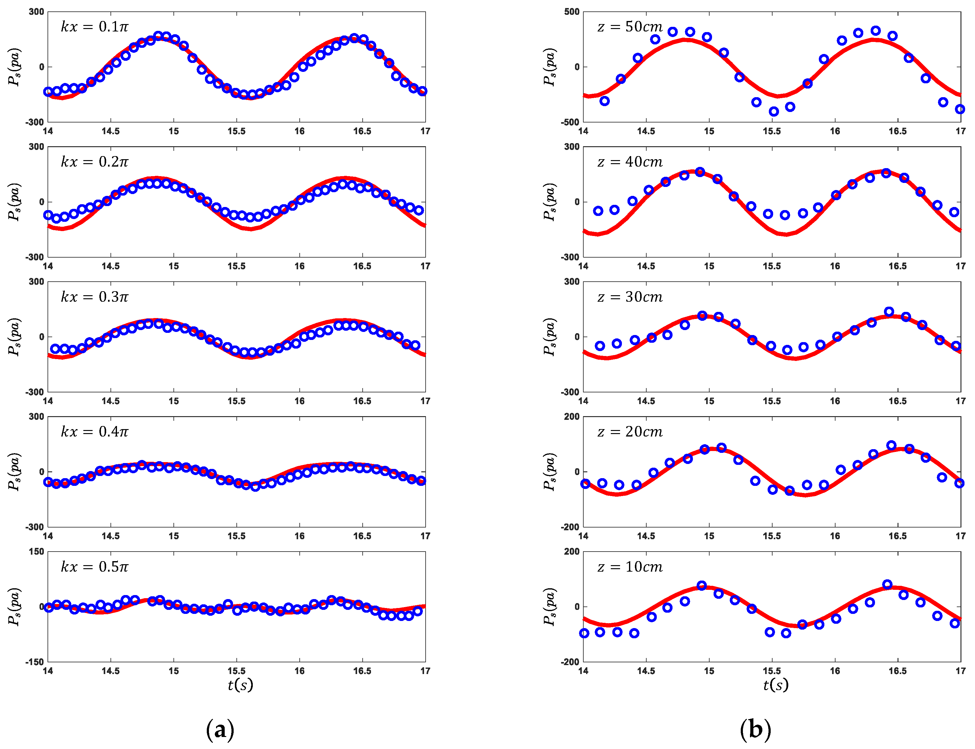
3.2. Validation for the Seabed Response

Tsai and Lee [27] conducted a series of experiments to investigate the sand bed response, induced by the standing wave. The details of the experiments can be found in Tsai and Lee [27]. A brief description is provided for the convenience and completeness (see Figure 3). The experimental wave flume was 100 m long, 2 m wide, and 2 m high. The water depth above the mudline was 45 cm, the wave period was 1.5 s and the wave height of the incident wave was 5.1 cm. The sandy soil was filled to a depth of 0.5 m and 2 m in length, in front of the wall. Five pore-water pressure transducers were installed vertically below the wall to measure the pore pressure and another five transducers were placed horizontally below the mudline. Figure 4 shows a comparison of the wave-induced pore pressure at ten pressure transducers, between the simulation and the measurement. It is seen from Figure 4 that the predicted pore pressure agrees well with those measured in the laboratory experiments.

4. Results

In this section, the validated PORO-WSSI II model is applied to investigate the effect of the rear reflection on the F–P resonance and the seabed response, due to the wave propagating over the multiple submerged breakwaters. The transmitted wave is confined to the region between the submerged breakwaters and the vertical structure. A sketch of the trapezoidal submerged breakwaters and the vertical structure is shown in Figure 5. The computational domain covers $-50\le x\le 50\mathrm{m}$ and $0\le z\le 1.0\mathrm{m}$. The wave-maker method, developed by Lin and Liu [41], is adopted to generate the desired wave at $x=-20\mathrm{m}$. The sponge layers are set on both sides of the numerical flume to eliminate the reflection wave. The water depth is $d=0.8\mathrm{m}$ and a trapezoidal shape is used with a fixed dimension of $h_s=0.4\mathrm{m}$, $W_b=2d=1.6\mathrm{m}$, and $W_t=0.5d=0.4\mathrm{m}$. The interval between the submerged breakwaters is $L_s=2.5d=2\mathrm{m}$. Two different cases are simulated, i.e., the wave trapping by a rigid breakwater in the presence of (i) two submerged breakwaters, (ii) three submerged breakwaters. The vertical breakwater is located at a resonator length $S/L=n/16$, where $L$ is the wave length, from the lee side of the latter submerged breakwater. The width of the rigid breakwater is $W=d=0.8\mathrm{m}$, and the height of the vertical structure is $h_v=1.25d=1.0\mathrm{m}$. More details of the wave conditions, soil properties, and structure characteristics are listed in

Table 1. Test conditions of the numerical simulations.

Mediums	Parameters
Wave	Wave height (m)	H	0.04
	Wave period (s)	T	1.29~3.73
Seabed	Porosity	ns	0.3
	Thickness (m)	h	10
	Permeability (m/s)	K	10−3
	Degree of saturation	Sr	1.0
	Poisson’s ratio	${\mu }_s$	1/3
Submerged breakwater	Porosity	n	0.3~0.5
	Mean grain size (m)	d50	0.076
	Shear modulus (N/m2)	G	109
	Poisson’s ratio	$\mu$	1/3

.

For the purpose of comparison, the parameters that are common in all simulation cases are given fixed moderate values. Each of which is changed for the corresponding effect on the wave interaction under discussion, while the other values are kept the same. In the case of the three submerged breakwaters ($m=3)$ backed by a rigid breakwater, the wave period is fixed as $T=3.16\mathrm{s}$ or $kd=0.6$, and the distance between the submerged breakwaters and the vertical structure keeps as $S/L=1.0$. The porosity of the submerged breakwaters is $n=0.5,$ unless otherwise stated. The model is subsequently run for each experimental case (see Table 1) for a duration of 100 wave periods. To allow the full interaction of the wave and the structure, only the simulation results of the last 50 wave periods are used for analysis, as suggested by Couston et al. [16].

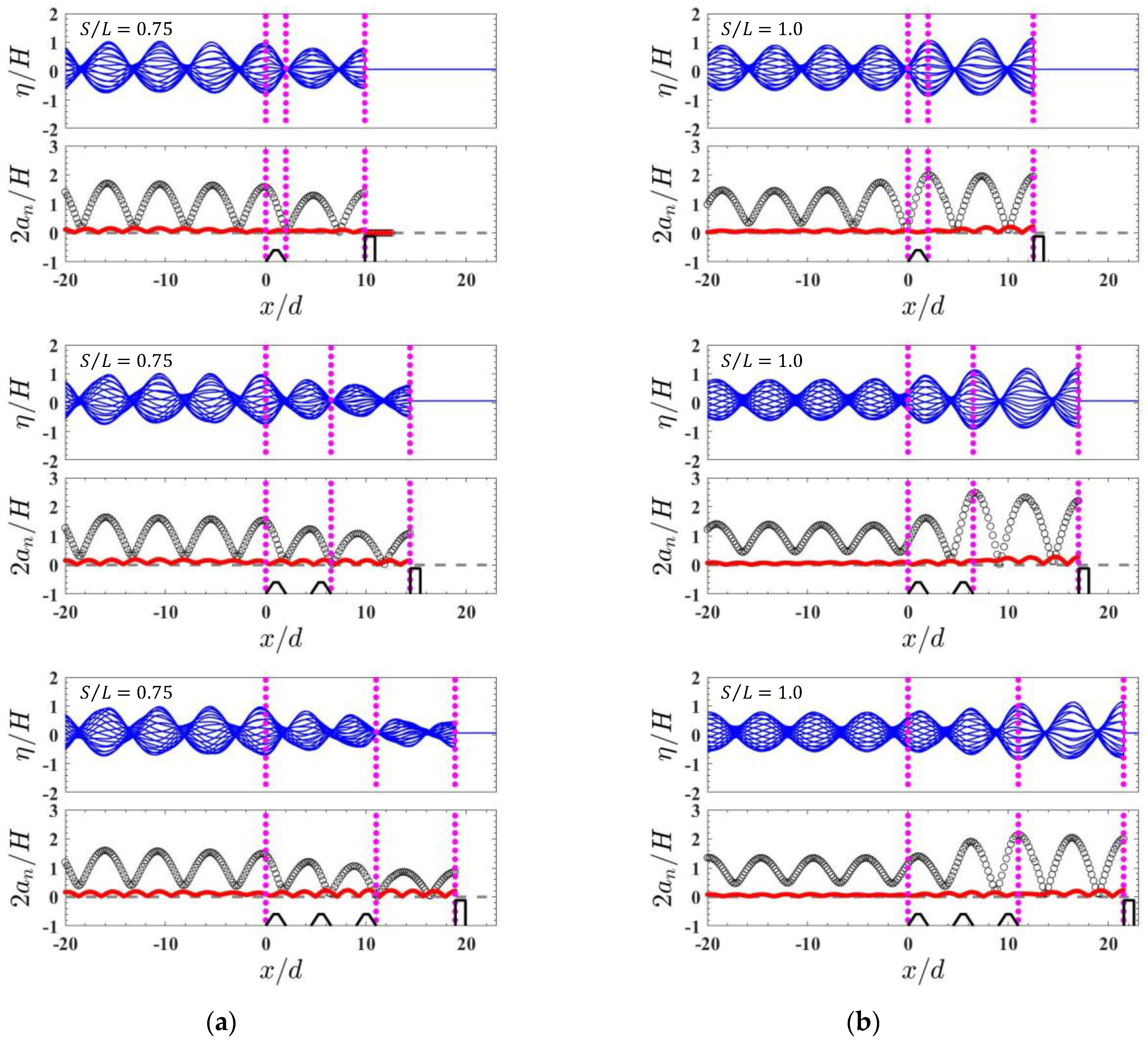
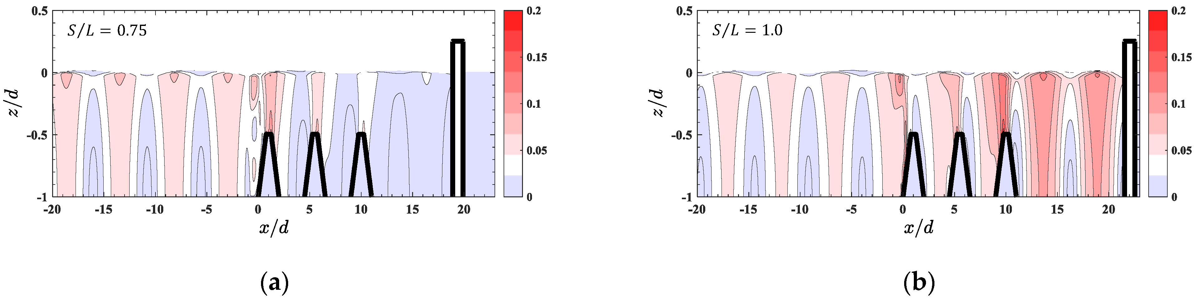
4.1. Wave Transformation

Figure 6 shows the numerical results for the temporal variation of the surface elevation and the spatial evolution of the harmonic amplitude under the Bragg resonance period, $kd=0.6$, with a different number of the submerged breakwaters and intervals S. It is seen that the partial standing waves are formed and the significant wave amplification or suppression can be observed between the breakwaters under the F–P resonance condition. With the increase of the interval between the breakwaters, it can be observed that two modes of the wave transformation exist. For Mode 1: most wave energy is reflected back to the open sea. Therefore, the displacement of the free surface decreases gradually from the area above the submerged breakwaters, and reaches a minimum between the submerged breakwater immediately after the submerged breakwaters, as shown in Figure 6a. It is noted that the amplitude of the fundamental harmonic component decreases from 1.92, 1.90, and 1.84, in the front of the outer submerged breakwater, respectively, to 1.88, 1.48, and 1.14, near the rigid breakwater. For Mode 2 $\left(\mathrm{at}S/L=\frac{8+8n}{16},\mathrm{or}\frac{9+8n}{16},n=0,1,2,3,\dots \right)$: the majority of the incident wave energy is trapped by the submerged breakwaters near a rigid breakwater. A F–P cavity is formed with the interference of the re-reflected water wave, by the frontal submerged breakwaters and the rear vertical breakwater. As shown in Figure 6b, the displacement of the free surface near the rigid breakwater is 1.2, 1.5, and 1.6 times higher than that in front of the outer submerged breakwater, where the amplitude of the fundamental harmonic component increases from 1.90, 1.78, and 1.66, to 2.38, 2.76, and 2.66, for m=1, 2, and 3, respectively. Comparing with the case with a breakwater (m=1), the additional submerged breakwater amplifies the interaction between the wave and the displacement of structures. More wave energy is reflected and trapped for the case with three breakwaters $\left(m=3\right)$ in Mode 1 and 2, respectively. To understand the basic mechanism of the wave evolution during the propagation, the spatial variation of the amplitude of the first two harmonics is decomposed in Figure 6. The amplitude of the fundamental harmonic component decays with the increase of the number of the submerged breakwaters. However, the amplitude of the higher harmonic component increases in front of the outer submerged breakwater, as well as near the rigid breakwater. This may be due to the generation of the higher-order harmonics by the nonlinear interaction between the incident wave and the structures, which means that the long period waves are distorted by the change of the bottom topography, and the nonlinear interaction between the wave and the structures is important. Taking $S/L=0.75$ as an example, the amplitude of the fundamental harmonic component decreases from 1.88 to 1.14 and the amplitude of the higher harmonic component increases from 0.144 to 0.196, near the rigid breakwater. This harmonic component’s increase is caused by the nonlinear interaction process with the wave energy transfer from the fundamental harmonic to the second harmonic.

To investigate more details about the wave energy transfer, the group velocity, one of the most important concepts in waves, is discussed. Based on the kinematic view, the group velocity can be defined as [42]

$$c_g=\frac{\partial \omega }{\partial k}=\frac{1}{2}\left[1+\frac{2kd}{\sinh 2kd}\right]\sqrt{\left(g/k\right)\tanh kd}$$

(21)

The group velocity also has a dynamic meaning of the velocity of the energy transport, which relies on the relation [42]

$$c_f=P/E$$

(22)

where $P$ is the wave energy flux and $E$ is the wave energy density. The wave energy flux and wave energy density are defined as [42]:

$$P=\frac{1}{T}{{\displaystyle \int }}_t^{t+T}{{\displaystyle \int }}_0^{d+\eta }u\left[p_d+\frac{1}{2}\rho \left(u^2+v^2\right)\right]d_z{d}_t$$

(23)

$$E=\frac{1}{T}{{\displaystyle \int }}_t^{t+T}{{\displaystyle \int }}_0^{d+\eta }\left[\rho g\left(z-d\right)+\frac{1}{2}\rho \left(u^2+v^2\right)\right]d_z{d}_t$$

(24)

Noted that in the limit of the non-dissipative progressive waves, the magnitude of $c_f$ is identifiable with $c_g$. Figure 7 shows the time history of the variation in the group velocity $c_f/c_g$ at the entrance of the three submerged breakwaters $\left(x/d=0\right),$ with a wave period of $T=3.16\mathrm{s}$. It is clearly seen that wave approaches to the entrance with the group velocity $c_f=c_g$ at $t/T=3$. As shown in Figure 7b, the steady state is reached after about 50 wave periods, which is quantitatively consistent with those observations made in previous studies [16], and the group velocity is stable at $c_f/c_g=0.55$.

Figure 8 shows the variation of the non-dimensional velocity of the energy transport $c_f/c_g$ with the resonator length under the Bragg resonance period $kd=0.6$. It is obvious that a strong positive transport velocity occurs in front of the first submerged breakwater. Therefore, most of the wave energy flows into the system, which consists of the submerged breakwaters and the rear vertical breakwater. With the wave energy transformation over the submerged breakwater, the velocity of the energy transport $c_f/c_g$ steps down to zero. Therefore, almost no energy transformation exists and a standing wave is formed between the submerged breakwaters and the vertical breakwater, which is also shown in Figure 6. As shown in Figure 8, the peak values of the transport velocity are 0.22, 0.36, and 0.47 at $S/L=0.75$ for m=1, 2, and 3, respectively. Compared to the case under Mode 1, the energy flux transports faster under Mode 2 and the peak values of the transport velocity are 0.30, 0.52, and 0.55 for m = 1, 2, and 3, respectively. The faster the wave energy flows in, the more energy is trapped and dissipated. Therefore, there are violent fluctuations near the vertical breakwater at $S/L=1.0$ (this is also seen in Figure 6b). The dissipation coefficient will be further discussed in the following sections.

The distribution of root-mean-square velocity magnitude (unit: m/s) around the breakwaters with a wave period of $T=3.16\mathrm{s},$ is plotted in Figure 9. Figure 9 shows that a significant velocity gradient occurs in the vicinity of the submerged breakwaters, especially near the front of the submerged breakwater. Both Mode 1 and Mode 2 are considered here. It is found that the distance between the submerged breakwaters and the vertical breakwater contributes a significant difference in the velocity field around the breakwaters. It is seen from Figure 9, that the flow velocity above the submerged breakwaters is higher than that of the adjacent area for Mode 1. This is because the existence of the submerged breakwaters partly reflects and dissipates the wave energy. Whereas in the case of the wave transforming under Mode 2, the breakwaters tend to trap the wave, thus enhancing the velocity near the vertical breakwater.

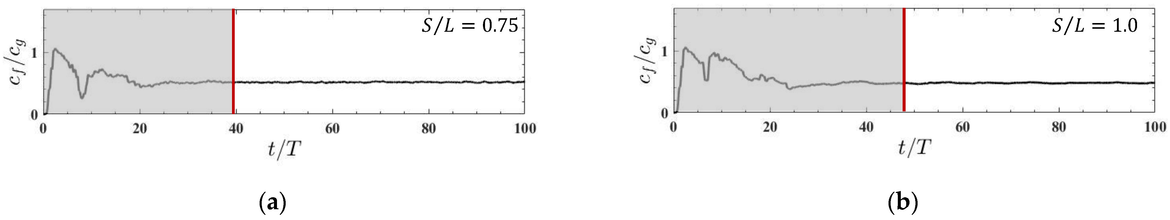
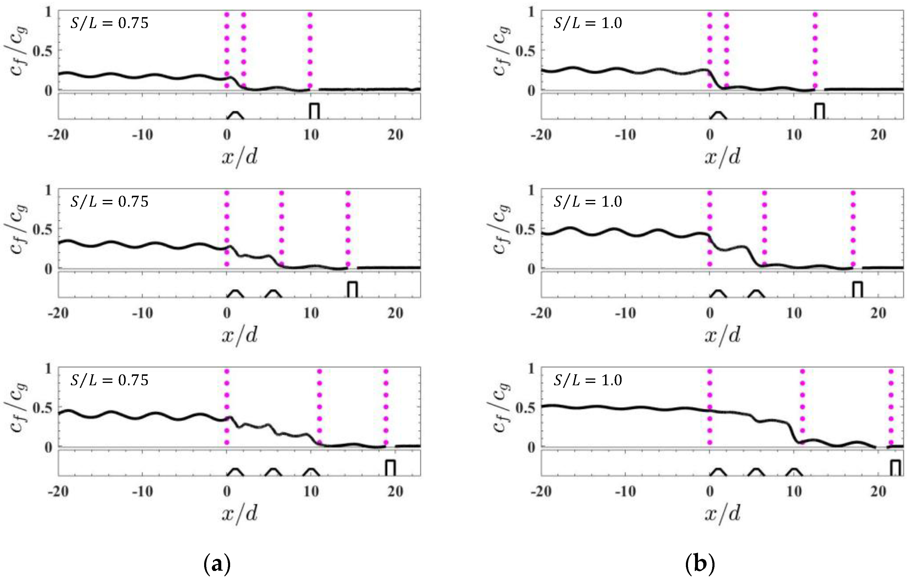
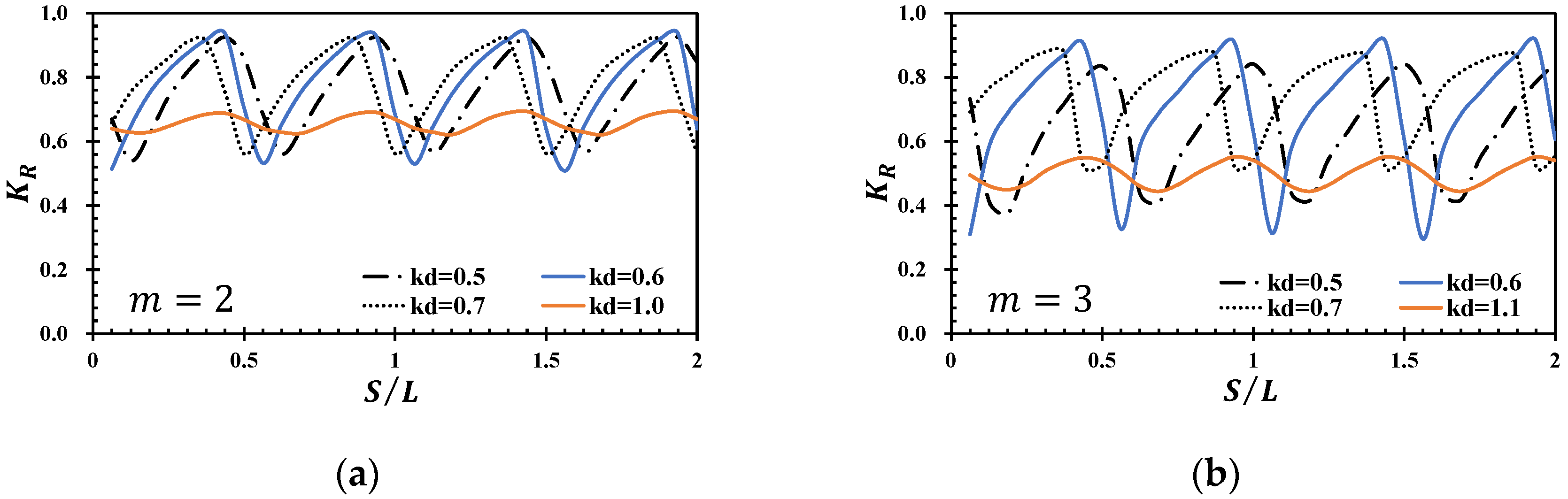
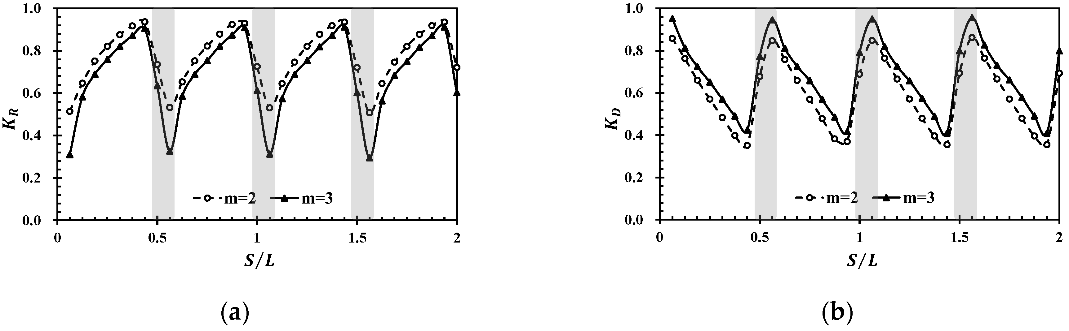
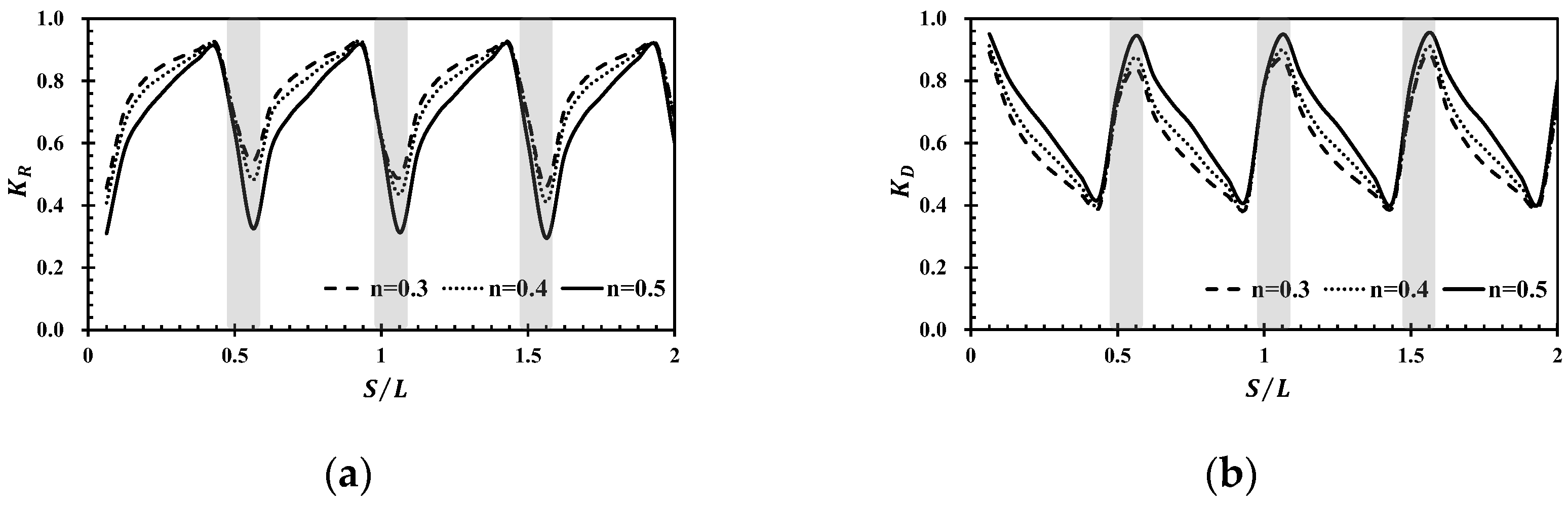
4.2. Wave Reflection and Dissipation Coefficients

Conventionally, the effectiveness of the coastal structures is estimated in terms of the wave reflection, transmission, and dissipation coefficients. The reflection $K_R=\frac{H_R}{H_I}$, is also obtained by the method of Goda and Suzuki [40], where $H_R$ is reflected by the wave height and $H_I$ is incident wave height.

Figure 10 shows the reflection coefficient $K_{R,}$ versus the resonator length $S/L,$ for the different values of the wave period $T$. It is seen from Figure 10, that the variation of $K_R$ is periodic. For the frontal weak reflection condition (e.g., $kd=1.0; m=2$ or $kd=1.1; m=3$), the reflection coefficient shows a slight oscillation with the resonator length $S/L$. However, the Bragg resonance coefficient plays a very significant role in trapping the waves by the submerged breakwaters. The reflection coefficient is more sensitive for the resonator length with the larger frontal Bragg reflection coefficient. Taking $m=2$ as an example, the amplitude of the fluctuation increases to 0.42 (at $kd=0.6$). Figure 10 also indicates that the locations of the minima have an obvious leftward shift with the increase of $kd$. This may be due to the change in the phase angle of the porous-effect in the submerged breakwaters.

Based on the principle of the energy conservation, the dissipation coefficient $K_D$ is related to the reflection coefficient and can be calculated as:

$$K_D=\sqrt{1-K_R^2}$$

(25)

Figure 11 shows the variation of the reflection coefficient $K_R$ and the dissipation coefficient $K_D$ with the resonator length under the Bragg resonance condition, $\mathrm{i}.\mathrm{e}.,kd=0.6$. The gray shadow is the phase where the wave transforms in Mode 2. It is seen that the reflection and dissipation coefficients vary periodically with the resonator length $S/L$ and each curve repeats itself in every half-wavelength. Figure 11 shows that the maxima $K_R$ takes place at $S/L=\frac{7+8n}{16}\left(n=0,1,2,3,\dots \right)$, which means that the wave transforms in Mode 1, and most of wave energy is reflected by the submerged breakwaters. The number of the submerged breakwaters $m$ has a great impact on the reflection and dissipation coefficients. Comparing these two lines, it is obvious that the large frontal Bragg reflection coefficient $(K_R=0.50; m=3$ in Figure 2$)$ results in a higher reflection extinction and a higher dissipation of the wave energy. Due to the wave energy dissipated by the additional submerged breakwater, the dissipation coefficient $K_D$ for $m=3,$ shows that it is larger than that for $m=2$, especially when the wave transforms in Mode 2. Unlike the traditional formula of the dissipation coefficient $K_D=\sqrt{1-K_R^2-K_T^2}$ [35], the dissipation coefficient defined in Equation (25) also shows the trapped wave energy re-dissipated by the frontal submerged breakwaters. The additional submerged breakwater enhances the process of re-dissipation. Therefore, the dissipation coefficient $K_D$ jumps obviously from 0.85 to 0.95 when the number of the submerged breakwaters increases at $S/L=\frac{9+8n}{16}\left(n=0,1,2,3,\dots \right)$.

It has been well-known that the wave energy dissipation is highly dependent on the breakwater porosity. The breakwater porosity is taken as $n=0.3,0.4\mathrm{and}0.5$ in this study, respectively, and its impact on the reflection and dissipation coefficients is shown in Figure 12. It can be seen that the obvious decline of the reflection coefficients $\left(K_R=0.54,0.48\mathrm{and}0.32\right)$ with the increase of the porosity $\left(n=0.3,0.4\mathrm{and}0.5\right),$ occurs at $S/L=\frac{9+8n}{16},\left(n=0,1,2,3,\dots \right)$. This indicates that the submerged breakwaters with a larger porosity $\left(n=0.5\right)$ provide more space for the flow development inside the submerged breakwaters, which leads to a higher energy dissipation. It implies that the wave period ($T$ or $kd$), the parameters of the submerged breakwaters ($m$ and $n$), and the reflectivity of the vertical structure, have a significant influence on the wave motion. The key to the qualitative change of the wave response in a trapping system is the phase of the rear reflection, relative to that of the arrays of the submerged breakwaters. Since the seabed response is mainly dominated by the wave motion [26], these four parameters may also affect the wave force exerting on the rigid breakwater and on the wave-induced seabed response.

Based on the above discussions, it can be concluded that the distance between the submerged breakwaters and the vertical breakwater has a significant influence on the wave transformation. This may further affect the shelter of the submerged breakwaters, which is part of the focus of this study and will be discussed in the following sections.

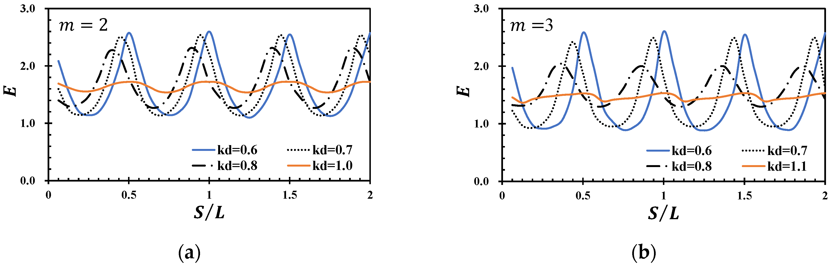
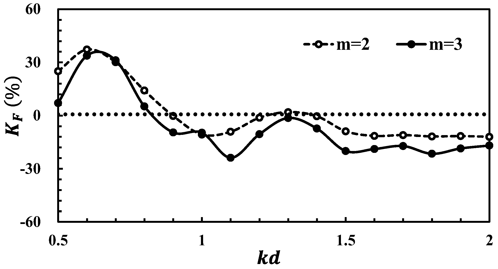
4.3. Enhancement Coefficient

Based on the above discussion, we can find the analogy between the water wave trapping mechanism and the F–P resonance in the optics. Without the consideration of the dissipation in the optics, the resonator length of the F–P resonance can be easily determined by the coefficient of the reflection or the transmission. For a given resonator length, the partial wave is reflected back, the trapped wave by the breakwaters constructively interferes and the F–P resonance condition is satisfied. In this study, the enhancement coefficient is defined by the amplitude of the water wave within the resonator in [16]:

$$E=\frac{H_T}{H_I}$$

(26)

where $H_T$ is the trapped wave height.

Figure 13 shows the variation of the enhancement coefficient $E$ with the resonator length $S/L,$ for the different values of the wave period $T$. Figure 13 shows that the highest $E$ occurs on the F–P resonance condition with the resonator length $S_T/L=\frac{8+8n}{16}+\theta ,\left(n=0,1,2,3,\dots \right)$, where $\theta$ is the phase shift. A leftward shift is observed and the phase $\theta$ changes significantly for the different wave periods. This is mainly due to the greater detuning frequency and the nonlinear interaction between the wave and porous structures. Comparing the two solid lines, it is clear that the large frontal Bragg reflection coefficient $(K_R=0.32,m=2;K_R=0.50,m=3$ in Figure 2$)$ results in a higher field enhancement between the breakwaters. The larger the trapped wave energy, the stronger the wave force acting on the vertical breakwater. This will be discussed in the following section.

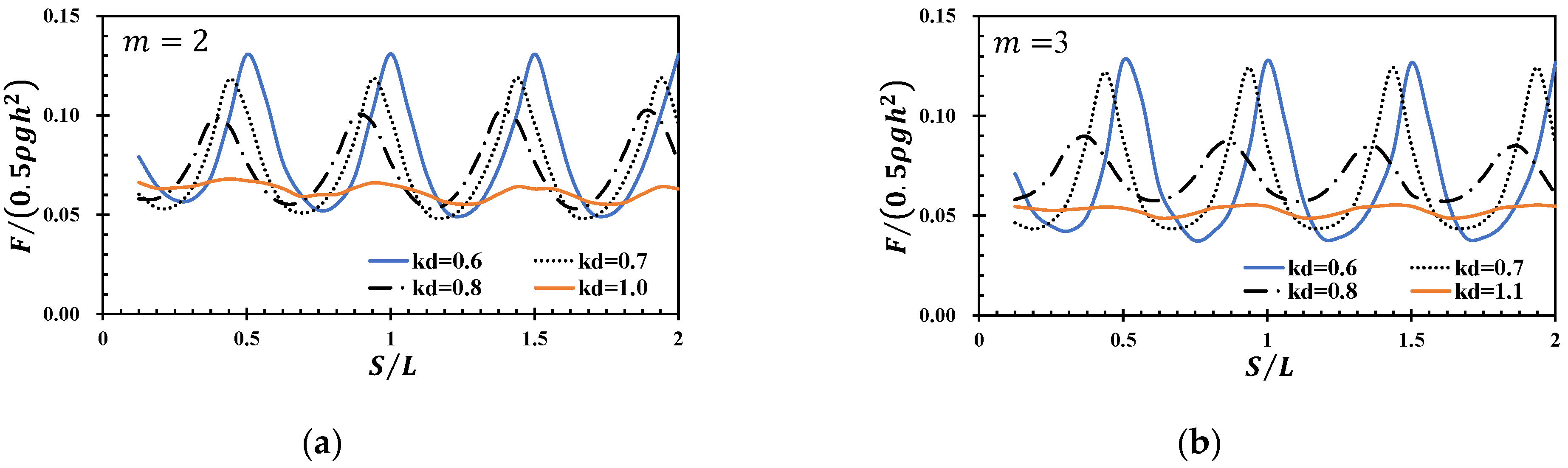
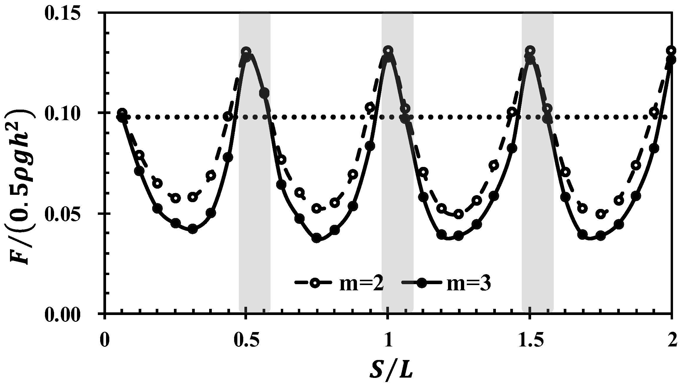
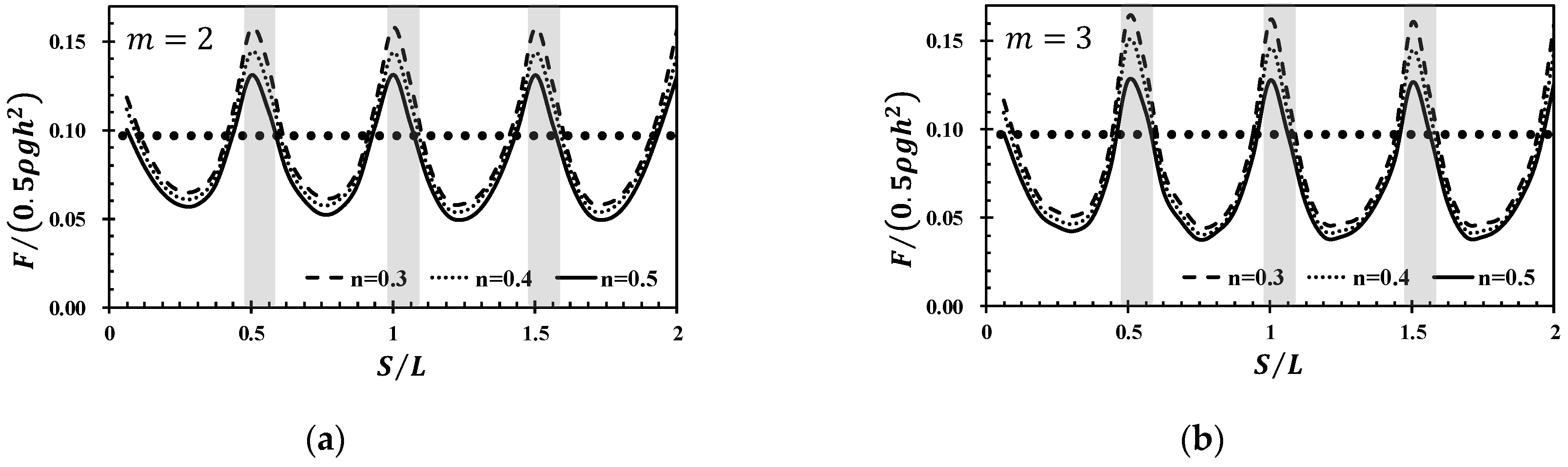
4.4. Pressure Drag

Determining the drag force acting on the vertical structure, is very important for the coastal structure design. Since the friction force is much smaller than the pressure force, only the horizontal hydrodynamic force ($F$) is considered here. It is computed by the pressure force acting on the vertical structure. In Figure 14, Figure 15, Figure 16 and Figure 17, the drag F is normalized by the hydrostatic pressure force $\left(=0.5\rho \mathrm{g}{h}^2\right)$ acting on the vertical breakwater. Figure 14 is the variation of the pressure force with the resonator length $S/L$ for the different wave periods. The periodic oscillation of the wave force is in phase with the enhancement coefficient. A left shift is clearly observed in the pressure force acting on the vertical structure. The phase of the maximum wave force shifts from $S_T/L=\frac{8+8n}{16}$ to $\frac{6+8n}{16}\left(n=0,1,2,3,\dots \right)$ with the greater detuning frequency. In addition, the maximum magnitude of the oscillation occurs at the Bragg resonance period $\left(kd=0.6\right)$. It is seen that with a relative increase in the detuning frequency relative to the Bragg resonance frequency, the fluctuation of the pressure force is weakened. For the case with two submerged breakwaters $\left(m=2\right)$, the fluctuation amplitude at $kd=0.7$ is only 85% of that at $kd=0.6$. Especially for the weak reflection condition, e.g., $kd=1.0;m=2$ or $kd=1.1;m=3$, the normalized wave force is almost close to a constant 0.064 or 0.053.

Figure 15 and Figure 16 show the wave force acting on the vertical breakwater with different structure configurations under the Bragg resonance period $\left(kd=0.6\right)$. In Figure 15 and Figure 16, the wave force acting on the vertical breakwater without other structures (dotted line) is also plotted to better analyze the shelter behind the submerged breakwaters. As shown in Figure 15, the presence of the submerged breakwaters may worsen the hazards under Mode 2 and the non-dimensional wave force rises to 0.13 at a strong F–P resonance trapping condition $\left(S_T/L=\frac{8+8n}{16},n=0,1,2,3,\dots \right)$, as most of the wave energy is trapped between the breakwaters (see Figure 6). In addition, there is a significant reduction of wave force, due to the additional submerged breakwater, under the condition of Mode 1. The minimum non-dimensional wave force, in the case $m=2$ with the optimal distance $S_o/L=\frac{4+8n}{16}\left(n=0,1,2,3,\dots \right)$, is 0.058, while it is 0.042, in the case with $m=3$. Unlike the reduction of the wave force by the additional submerged breakwater, the submerged breakwaters with a larger porosity can effectively shelter the rear breakwater (see Figure 16). This implies the benefit of using the submerged breakwater with a larger porosity. Taking $m=3$ as an example, the maximum non-dimensional wave force decreases from 0.16 to 0.13 under the strong F–P resonance trapping condition. However, the vertical breakwater still suffers from the stronger wave impact than that without frontal submerged breakwaters under the F–P resonance condition.

Based on the above discussion, the presence of the frontal submerged breakwaters may worsen the hazards under the F–P resonance condition. To estimate the shelter under this extreme condition, the coefficient of the wave force is obtained using the formula $K_F=\frac{F_T-F_{isolate}}{F_{isolate}}\times 100\%$, where $F_T$ and $F_{isolate}$ are, respectively, the wave force acting on the vertical breakwater with the frontal two or three submerged breakwaters, and without the submerged breakwaters under the F–P resonance condition.

Figure 17 depicts the variation of $K_F$ with the non-dimensional wave number $kd$ for the different structure configurations. Usually, the coefficient of the wave force is negative, due to the reflection and dissipation of the frontal submerged breakwaters. However, under the condition near the first Bragg resonance $kd=0.6$, the protection from the submerged breakwaters can be absolutely broken down and the maxima of the wave force on the vertical breakwater is 37% or 33% greater than that on the only vertical breakwater for $m=2$ or $3$, respectively. It should be noticed that $K_F$ almost approaches to zero near the second Bragg resonance $kd=1.3$. The great Bragg reflection of the submerged breakwaters generates a stronger wave force. When the period of the incident wave is short $\left(kd>1.5\right)$, the primary mechanism of the wave-submerged breakwaters interaction transfers from wave scattering to reflection and dissipation, and the ratio of the wave force $K_F$ is close to a constant $-11.6\%$ and $-18.6\%$ for $m=2$ or $3$, respectively. Thus, the arrays of the submerged breakwaters can either provide shelter or worsen the hazards for the rear structure, depending on the number of the submerged breakwaters, wave periods, and the condition of the rear reflection.

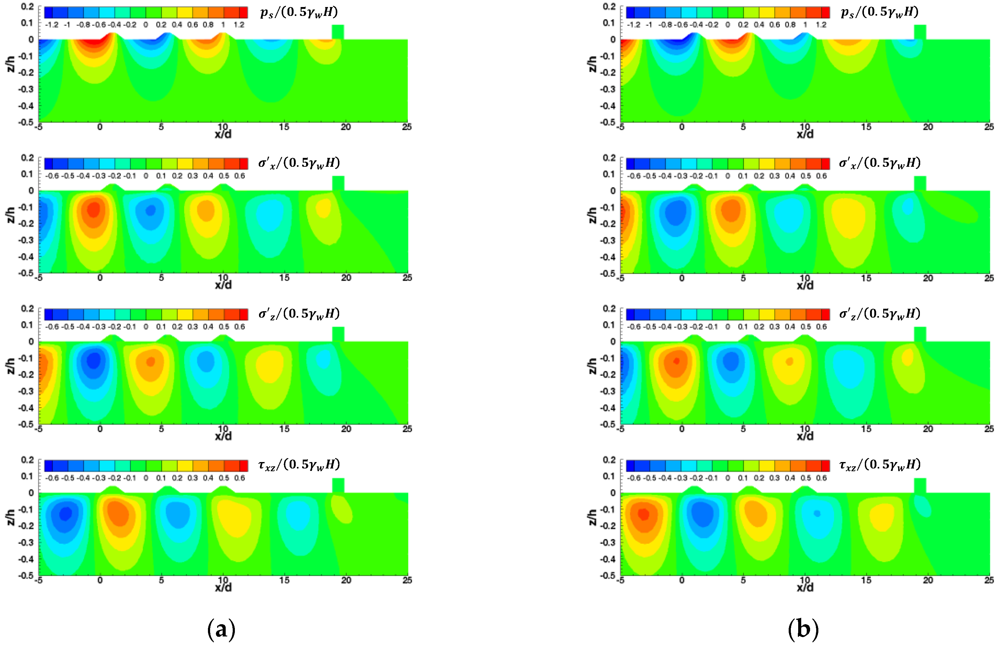
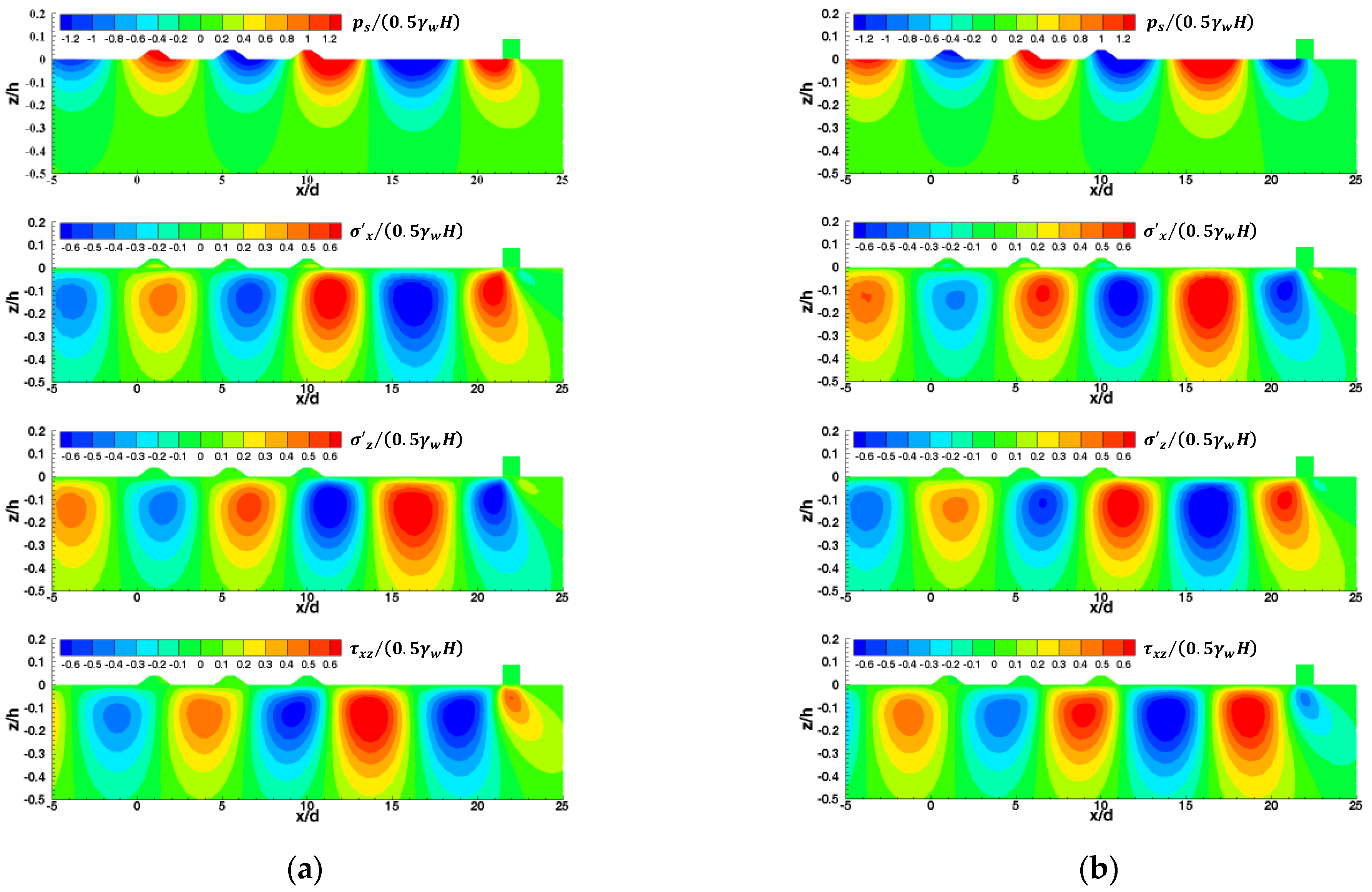
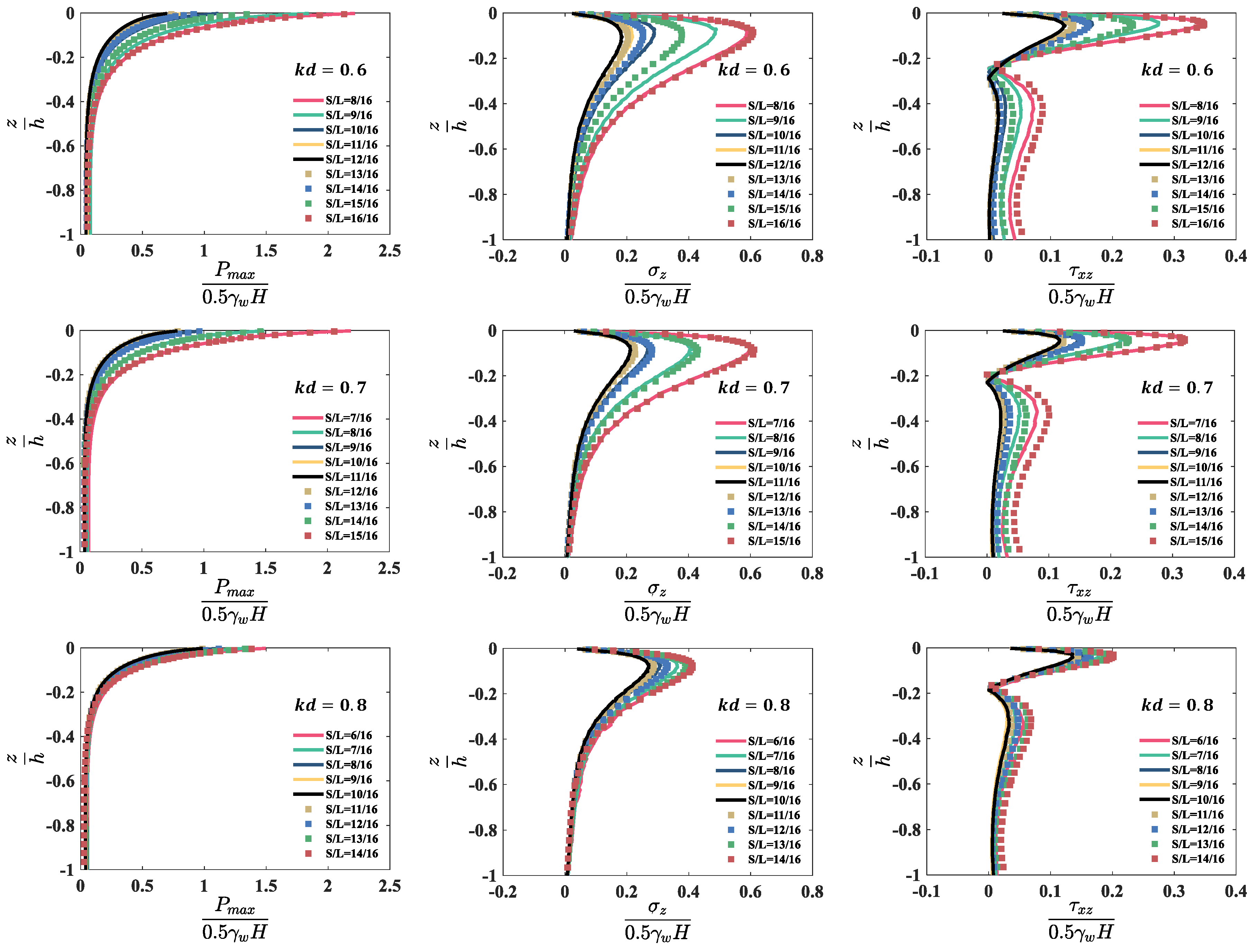
4.5. Dynamic Response of the Seabed

Wave propagating over the seabed will induce an excess pore pressure and a consequent decrease of the effective stress around structures. Figure 18 and Figure 19 display snapshots of the dynamic pore pressures, the effective normal stresses, and the shear stress at two typical times around the breakwaters with $kd=0.6$ under two different Modes. The wave pressure is transmitted into the seabed foundation through the soil skeleton and the pore fluid. As shown in these figures, the wave-induced pore pressure, the effective normal stresses, and the shear stress are negligible in the region below $z/H_s<-0.5$. The soil around the vertical breakwater is dilated or contracted under the cyclic wave loading. It is noted that the pore pressure $\left(p_s\right)$ is positive, the dynamic $\sigma {\prime }_x$ is tensile, and $\sigma {\prime }_z$ is compressive near the vertical breakwater under the wave crest $\left(t/T=0.25\right)$. A reverse trend can be found under the wave trough $\left(t/T=0.75\right)$. Another interesting observation from these figures is that the magnitude of the wave-induced pore pressure and the dynamic stresses are larger under Mode 2, especially around the vertical breakwater. The strong pore pressure is more likely to cause the liquefaction when there is a wave trough under Mode 2.

Figure 20 is the vertical distribution of the wave-induced pore pressure $p_{max}/\left(0.5{\gamma }_{w}H\right)$ and the dynamic stresses for the various resonator lengths below the toe of the vertical breakwater (the leading edge of the vertical breakwater) for $m=3$. The vertical distribution of the pore pressure and the effective stresses below the toe of the vertical breakwater also oscillate with an interval $\Delta S/L=8/16$ cycle. Taking $kd=0.6$ as an example, the pore pressure and the dynamic stresses decrease until $S/L=12/16$ and then increase with the increase of the distance $S/L$. Finally, the vertical distribution at $S/L=16/16$ shows the same trend as that at $S/L=8/16$, which is in phase with the enhancement coefficient. This indicates that the resonator length $S/L$ is a key parameter for the protection of the rear structure or the seabed foundation. A left shift in Figure 20 is also shown. The maxima wave-induced pressure occurs at the resonator length $S/L=16/16$, $15/16,$ and $14/16,$ under different wave periods $(kd=0.6$, $0.7,$ and $0.8)$. With the greater detuning frequency, the re-reflection caused by the submerged breakwaters is too weak to affect the wave transformation. Consequently, the magnitude of the pore pressure and the dynamic stresses only show a slight oscillation (see $kd=0.8$).

To further investigate the shelter of the submerged breakwaters, we examine the vertical distributions of the pore pressure, the effective normal stress and the shear stress below the toe of the vertical breakwater where the seabed instability is most likely to take place. Two conditions, namely $S_o/L=12/16$ and $S_T/L=16/16$, are considered in Figure 21 and Figure 22. As illustrated in Figure 21 and Figure 22, the small magnitudes of the pore pressures and the effective stresses appear at the optimal distance $S_o/L=12/16$, while the large magnitudes occur at $S_T/L=16/16,$ in comparison with that without the submerged breakwaters, especially at the upper part of the seabed. Figure 21 indicates that an additional breakwater $\left(m=3\right)$ has an impact on the seabed response. As shown in the figure, the value of $p_{max}/\left(0.5{\gamma }_{w}H\right)$ at the seabed, in the case with $\left(m=2\right)$ and $\left(m=3\right),$ is smaller than those in the case with the rigid breakwater, only, under the condition of $S_o/L=12/16$. Unlike the condition of Mode 1 $\left(S_o/L=12/16\right)$, the values of $p_{max}/\left(0.5{\gamma }_{w}H\right)$, $\sigma {\prime }_z/\left(0.5{\gamma }_{w}H\right),$ and ${\tau }_{xz}/\left(0.5{\gamma }_{w}H\right),$ for m=3 are the same as those for $m=2$ under the condition of Mode 2 $\left(S_T/L=16/16\right)$. Figure 22 also shows that the value of the wave-induced pore pressure and the effective stresses under both Modes increases with the decrease of the porosity of the submerged breakwater, leading to the likelihood of the seabed liquefaction, which is discussed below.

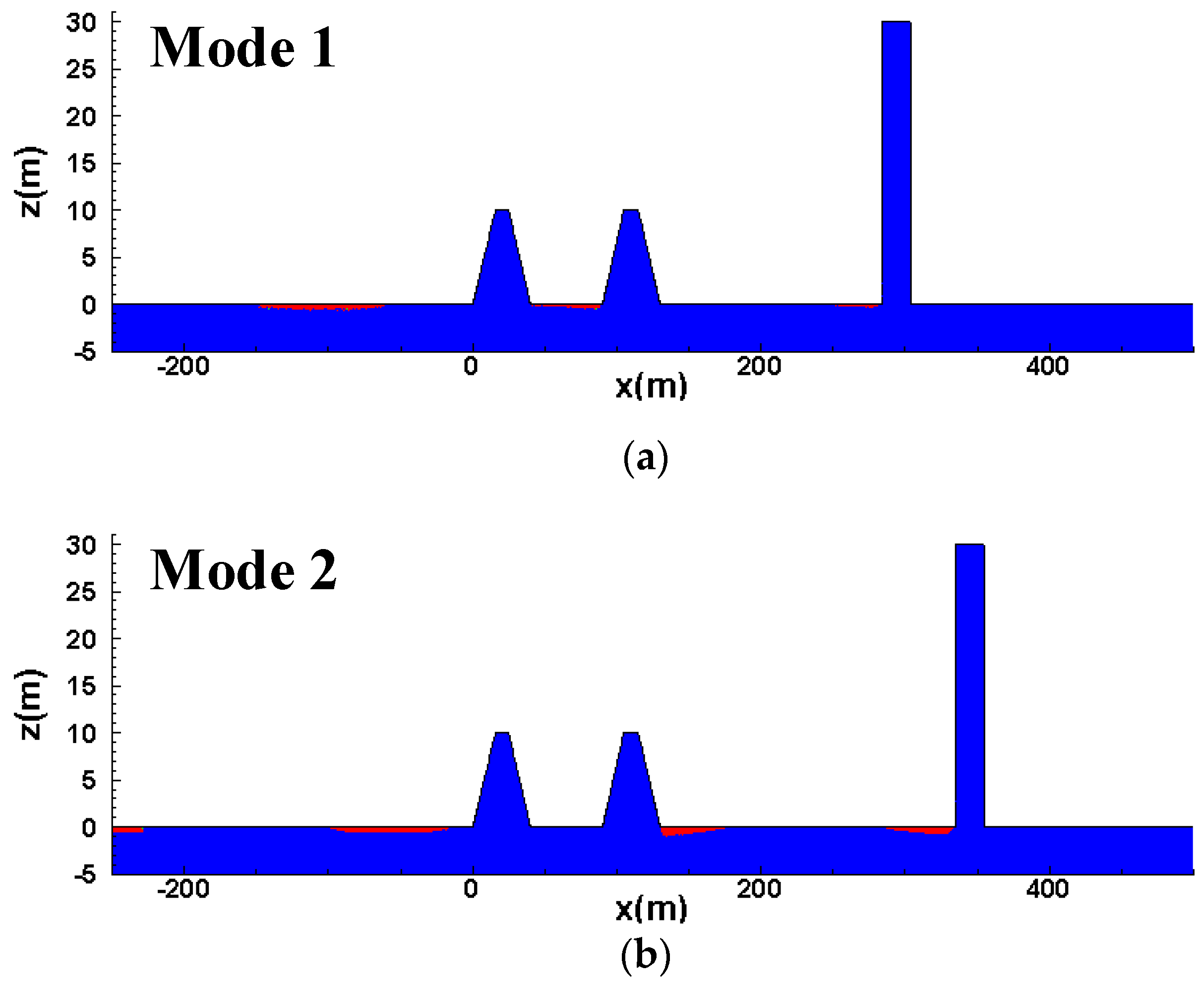
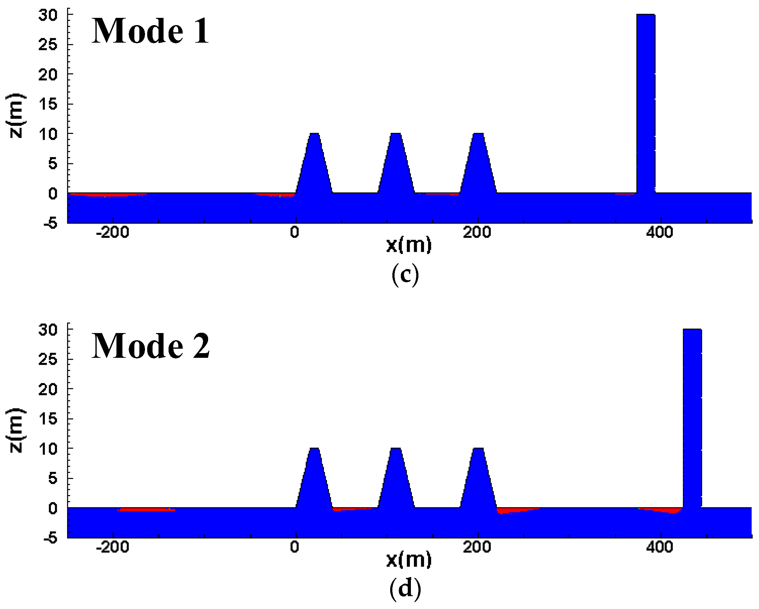
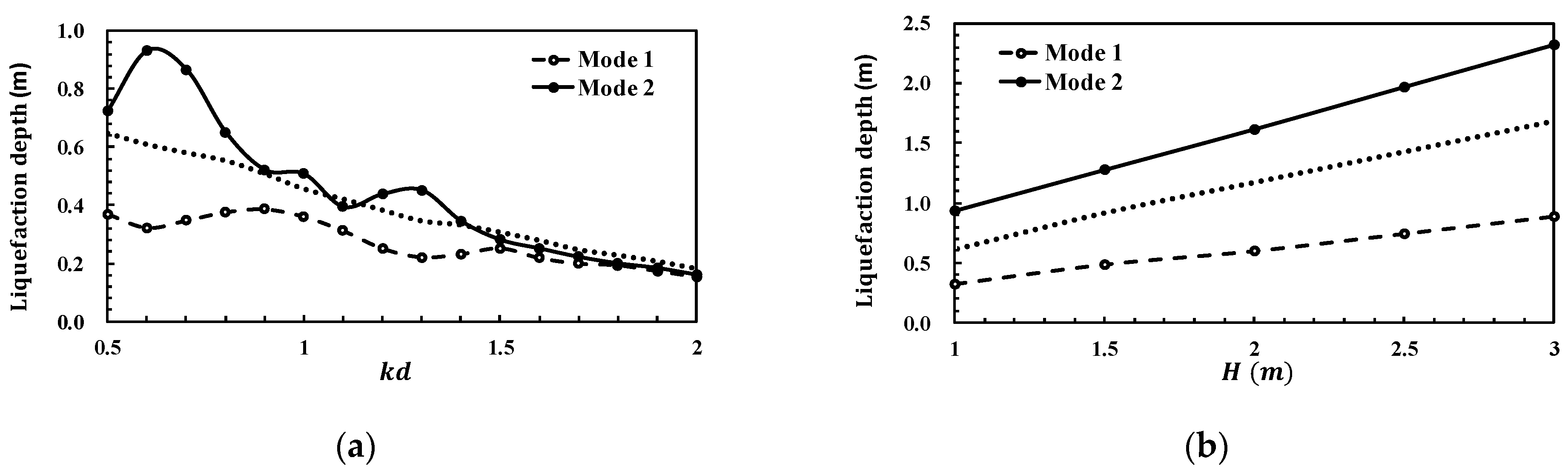
4.6. Liquefaction

The liquefaction is an extreme form of the seabed instability. When the pore pressure in the non-cohesive soil keeps increasing, until the effective stress becomes zero, the soil loses its structure strength and the liquefaction occurs. Therefore, the criteria for liquefaction is that the effective stress becomes zero [43]. However, this criterion is only applicable to the cases without structures. For the case with the breakwater, the criterion can be modified as [13]:

$${\sigma }_z^{\prime }+\left|{\sigma }_{z0}^{\prime }\right|\le 0$$

(27)

where the ${\sigma }_{z0}^{\prime }$ is the vertical effective stress at the initial consolidation state.

This section is on a larger case scale, with a domain 25 times larger in dimension, than that of the previous laboratory case (see Figure 23 and Figure 24). Based on the above discussion, the vertical breakwater may experience the seabed instability at $S/L=16/16$ under a strong F–P resonance trapping condition. Therefore, the simulated conditions are: wave height $H=1.0\mathrm{m}$, wave period $T=15.5\mathrm{s}$, and still water depth $d=20.0\mathrm{m}$, which will satisfy $kd=0.6$. The seabed parameters are: soil permeability $K={10}^{-3}$ m/s and the degree of saturation $S_r=0.95$. As discussed above, for both the Mode 1 and Mode 2, the wave will transform as a standing wave. Therefore, we focus on two typical times $t/T=0.25\mathrm{and}0.75$. Based on the criterion given by Equation (27), Figure 23 and Figure 24 show the wave-induced liquefaction potential around the breakwaters at two typical times. As shown in the figures, the liquefaction area appears in the zone near the seabed surface and its distribution is closely related to the dynamic loading. The results presented in Figure 23 and Figure 24 confirm that the momentary liquefaction can only occur under the wave troughs, due to the wave-induced negative vertical normal stress $\sigma {\prime }_z$. It is well known that the wave period has a significant impact on the distribution of the wave trough in a standing wave system. Therefore, the wave period is one of the important factors that play an important role in the location of the wave-induced liquefaction. Furthermore, the liquefaction does not occur in the seabed under the structures, due to the large initial stress induced by the consolidation process. It is worth noting that the distance between the submerged breakwaters and the vertical structure, has a significant impact on the distribution of the wave-induced maximum liquefaction area. As shown in Figure 23b, under Mode 1, most of wave is reflected back to the sea, and the maximum liquefaction depth normally occurs in front of the first submerged breakwater $\left(x=0\mathrm{m}\right)$. However, the maximum liquefaction area under Mode 2 significantly differs from that under Mode 1. The soil around the vertical breakwater $\left(x=425\mathrm{m}\right)$ liquefies with a potential depth $l_d=0.93\mathrm{m}$ under Mode 2 in Figure 24b. This implies that the seabed around the vertical breakwater is highly vulnerable to the momentary liquefaction under Mode 2.

At the typical time $t/T=0.75$, the liquefaction zone is very close to the foundation of the vertical breakwater, which may cause the instability of the foundation. Therefore, we will further investigate the development of liquefaction near the vertical breakwater. Figure 25 shows the wave-induced maximum liquefaction areas for the different breakwater numbers. Under Mode 1, the liquefaction depth $l_d$ decreases from $0.41\mathrm{m}$ to $0.32\mathrm{m},$ with the additional submerged breakwater. However, a higher liquefaction potential ($l_d=0.93\mathrm{m}$) near the vertical breakwater occurs in the case $m=3$ when the wave transforms under Mode 2, indicating that the construction of the third submerged breakwater may enhance the seabed instability around the vertical breakwater under the F–P resonance condition.

Figure 26 shows the maximum liquefaction depth in the vicinity of the vertical breakwater for the various conditions. Based on the above discussion, the wave-induced seabed response is in phase with the wave force. In other words, the maximum liquefaction depth and wave force occur under the same configuration $\left(S_T/L\right)$. Therefore, the resonator lengths $S_o/L$ and $S_T/L$ are chosen to be representative of Modes 1 and 2. It is seen from Figure 26 that the trapped wave under Mode 2 tends to enhance the potential of the maximum liquefaction depth, whereas the wave transformed under Mode 1 can effectively suppress this to some extent, thus comparing the case with the one with the vertical breakwater condition, only. This implies that the resonator length significantly affects the liquefaction depth around the vertical breakwater, especially close to the resonance period. Comparing the case with the rigid breakwater condition, only, the frontal three submerged breakwaters can reduce $46\%$ or strengthen $54\%$ the liquefaction depth under the Bragg resonance period $kd=0.6$. However, when the period of the incident wave is short $\left(\mathrm{e}.\mathrm{g}.kd\ge 1.5\right)$, the reflection and dissipation of the submerged breakwaters are more important than the Bragg resonance, and the liquefaction depth shows almost the same value.

5. Conclusions

In this study, based on the VARANS equations and Biot’s “$u_s-p_s$” approximation theory, an integrated model has been developed to quantitatively investigate the wave trapping under the F–P resonance condition. The performance of the double and triple submerged breakwaters is evaluated by examining the reflection, dissipation, and enhancement coefficients. The wave force and the wave-induced seabed response around the vertical breakwater are analyzed. From the present study, the following conclusions can be drawn:

• The presence of the submerged breakwaters in front of the vertical breakwater can either provide shelter or worsen the hazards, depending on the condition of the vertical breakwater reflection. The relative distance between the breakwaters determines how the wave energy is transferred locally, and the two Modes of wave transformation can be clarified: wave reflection and wave trapping. Reflection and dissipation of wave energy by frontal submerged breakwaters cause the magnitude of the flow velocity to decrease under Mode 1, and trapping of wave energy cause the magnitude to increase under Mode 2, at the back side of the submerged breakwaters;
• Trapping more wave energy under the F–P resonance condition leads to a smaller reflection coefficient, but also to a larger dissipation, enhancement coefficients, wave force, wave-induced pore pressure, and dynamic stresses. The presence of the submerged breakwaters tends to enhance the wave force and the potential of the maximum liquefaction depth in the vicinity of the vertical breakwater, comparing this with the case with the vertical breakwater condition, only;
• With the consideration of the bottom friction and the viscous dissipation, the reflection and dissipation coefficients are out of phase with the enhancement coefficient;
• The enhancement coefficient is in phase with the wave force, the wave-induced pore pressure, and the dynamic stresses. A strong amplification or damping is achieved. The optimal distance is $S_o/L=\frac{4+8n}{16} \left(n=0,1,2,3,\dots \right)$ for the Bragg resonance period, and the shifts to the left with the increase of $kd$. With the greater detuning frequency, the reflection and dissipation of the breakwaters are more important than the F–P resonance;
• The result reveals that triple submerged breakwaters with a high porosity is the most effective configuration in reducing the wave energy and to shelter the backward structure. The dissipation coefficient becomes larger as the presence of an additional submerged breakwater, hence the forced action on the vertical breakwater, the dynamic stresses, and the maximum liquefaction depth around the vertical breakwater, become smaller, especially under Mode 1. Increasing the porosity of the submerged breakwaters can also induce more significantly wave dissipation. Following a full wave-structure interaction, the magnitude of the wave force and the dynamic stresses within the seabed decreases with the increase of the porosity of the submerged breakwaters, especially under Mode 2.

References

- Jeng, D.-S.; Schacht, C.; Lemckert, C. Experimental Study on Ocean Waves Propagating over a Submerged Breakwater in Front of a Vertical Seawall. Ocean Eng. 2005, 32, 2231–2240. [Google Scholar] [CrossRef]
- Gao, J.; Ma, X.; Zang, J.; Dong, G.; Ma, X.; Zhu, Y.; Zhou, L. Numerical Investigation of Harbor Oscillations Induced by Focused Transient Wave Groups. Coast. Eng. 2020, 158, 103670. [Google Scholar] [CrossRef]
- Heathershaw, A.D. Seabed-Wave Resonance and Sand Bar Growth. Nature 1982, 296, 343–345. [Google Scholar] [CrossRef]
- Mei, C.C. Resonant Reflection of Surface Water Waves by Periodic Sandbars. J. Fluid Mech. 1985, 152, 315–335. [Google Scholar] [CrossRef]
- Gao, J.; Ma, X.; Dong, G.; Chen, H.; Liu, Q.; Zang, J. Investigation on the Effects of Bragg Reflection on Harbor Oscillations. Coast. Eng. 2021, 170, 103977. [Google Scholar] [CrossRef]
- Behera, H.; Khan, M.B.M. Numerical Modeling for Wave Attenuation in Double Trapezoidal Porous Structures. Ocean Eng. 2019, 184, 91–106. [Google Scholar] [CrossRef]
- Davies, A.G.; Heathershaw, A.D. Surface-Wave Propagation over Sinusoidally Varying Topography. J. Fluid Mech. 1984, 144, 419–443. [Google Scholar] [CrossRef]
- Liu, Y.; Yue, D.K.P. On Generalized Bragg Scattering of Surface Waves by Bottom Ripples. J. Fluid Mech. 1998, 356, 297–326. [Google Scholar] [CrossRef]
- Mase, H.; Oki, K.; Kitano, T.; Mishima, T. Experiments on Bragg Scattering of Waves due to Submerged Breakwaters. Coast. Struct. 2000, 99, 659–665. [Google Scholar]
- Cho, Y.-S.; Yoon, S.B.; Lee, J.-I.; Yoon, T.-H. A Concept of Beach Protection with Submerged Breakwaters. J. Coast. Res. 2001, 34, 671–678. [Google Scholar]
- Cho, Y.-S.; Lee, J.-I.; Kim, Y.-T. Experimental Study of Strong Reflection of Regular Water Waves over Submerged Breakwaters in Tandem. Ocean Eng. 2004, 31, 1325–1335. [Google Scholar] [CrossRef]
- Jeon, C.-H.; Cho, Y.-S. Bragg Reflection of Sinusoidal Waves Due to Trapezoidal Submerged Breakwaters. Ocean Eng. 2006, 33, 2067–2082. [Google Scholar] [CrossRef]
- Zhang, J.-S.; Jeng, D.-S.; Liu, P.L.-F.; Zhang, C.; Zhang, Y. Response of a Porous Seabed to Water Waves over Permeable Submerged Breakwaters with Bragg Reflection. Ocean Eng. 2012, 43, 1–12. [Google Scholar] [CrossRef]
- Kirby, J.T.; Anton, J.P. Bragg Reflection of Waves by Artificial Bars. Coast. Eng. 1990, 1991, 757–768. [Google Scholar] [CrossRef]
- Yu, J.; Mei, C.C. Do Longshore Bars Shelter the Shore? J. Fluid Mech. 2000, 404, 251–268. [Google Scholar] [CrossRef]
- Couston, L.-A.; Guo, Q.; Chamanzar, M.; Alam, M.-R. Fabry-Perot Resonance of Water Waves. Phys. Rev. E 2015, 92, 043015. [Google Scholar] [CrossRef] [PubMed] [Green Version]
- Terrett, F.L.; Osorio, J.D.C.; Lean, G.H. Model Studies of a Perforated Breakwater. In Coastal Engineering 1968; American Society of Civil Engineers: London, UK, 1969; pp. 1104–1120. [Google Scholar] [CrossRef]
- Chwang, A.T. A Porous-Wavemaker Theory. J. Fluid Mech. 1983, 132, 395–406. [Google Scholar] [CrossRef]
- Jeng, D.-S.; Ye, J.-H.; Zhang, J.-S.; Liu, P.L.-F. An Integrated Model for the Wave-Induced Seabed Response around Marine Structures: Model Verifications and Applications. Coast. Eng. 2013, 72, 1–19. [Google Scholar] [CrossRef]
- Sumer, B.M. Liquefaction around Marine Structures; Advanced Series on Ocean Engineering; World Scientific: Singapore; Hackensack, NJ, USA, 2014. [Google Scholar]
- Lin, Z.; Guo, Y.; Jeng, D.; Liao, C.; Rey, N. An Integrated Numerical Model for Wave–Soil–Pipeline Interactions. Coast. Eng. 2016, 108, 25–35. [Google Scholar] [CrossRef] [Green Version]
- Zhai, Y.; Zhang, J.; Jiang, L.; Xie, Q.; Chen, H. Experimental Study of Wave Motion and Pore Pressure Around a Submerged Impermeable Breakwater in a Sandy Seabed. Int. J. Offshore Polar Eng. 2018, 28, 87–95. [Google Scholar] [CrossRef]
- Zhang, J.; Tong, L.; Zheng, J.; He, R.; Guo, Y. Effects of Soil-Resistance Damping on Wave-Induced Pore Pressure Accumulation around a Composite Breakwater. J. Coast. Res. 2018, 34, 573. [Google Scholar] [CrossRef]
- Mizutani, N.; Mostafa, A.M. Nonlinear Wave-Induced Seabed Instability Around Coastal Structures. Coast. Eng. J. 1998, 40, 131–160. [Google Scholar] [CrossRef]
- Hur, D.-S.; Kim, C.-H.; Kim, D.-S.; Yoon, J.-S. Simulation of the Nonlinear Dynamic Interactions between Waves, a Submerged Breakwater and the Seabed. Ocean Eng. 2008, 35, 511–522. [Google Scholar] [CrossRef]
- Zhang, J.-S.; Jeng, D.-S.; Liu, P.L.-F. Numerical Study for Waves Propagating over a Porous Seabed around a Submerged Permeable Breakwater: PORO-WSSI II Model. Ocean Eng. 2011, 38, 954–966. [Google Scholar] [CrossRef]
- Tsai, C.-P.; Lee, T.-L. Standing Wave Induced Pore Pressures in a Porous Seabed. Ocean Eng. 1995, 22, 505–517. [Google Scholar] [CrossRef]
- Tong, L.; Zhang, J.; Zhao, J.; Zheng, J.; Guo, Y. Modelling Study of Wave Damping over a Sandy and a Silty Bed. Coast. Eng. 2020, 161, 103756. [Google Scholar] [CrossRef]
- Hsu, T.-J.; Sakakiyama, T.; Liu, P.L.-F. A Numerical Model for Wave Motions and Turbulence Flows in Front of a Composite Breakwater. Coast. Eng. 2002, 46, 25–50. [Google Scholar] [CrossRef]
- Lin, P.; Liu, P.L.-F. A Numerical Study of Breaking Waves in the Surf Zone. J. Fluid Mech. 1998, 359, 239–264. [Google Scholar] [CrossRef]
- Andersen, O.H. Flow in Porous Media with Special Reference to Breakwater Structures. Ph.D. Thesis, Hydraulics & Coastal Engineering Laboratory, Department of Civil Engineering, Aalborg University, Aalborg, Denmark, 1994. [Google Scholar]
- Fair, G.M. Water and Wastewater Engineering; Volume 2. Water Purification and Wastewater Treatment and Disposal; Wiley: New York, NY, USA, 1968. [Google Scholar]
- Kozeny, J. Ueber Kapillare Leitung Des Wassers Im Boden. Stizungsber Akad. Wiss., Wien,. 1927, 136, 271–306. [Google Scholar]
- Liu, P.L.-F.; Lin, P.; Chang, K.-A.; Sakakiyama, T. Numerical Modeling of Wave Interaction with Porous Structures. J. Waterw. Port Coast. Ocean Eng. 1999, 125, 322–330. [Google Scholar] [CrossRef]
- Lin, P.; Karunarathna, S.A. Numerical Study of Solitary Wave Interaction with Porous Breakwaters. J. Waterw. Port Coast. Ocean Eng. 2007, 133, 352–363. [Google Scholar] [CrossRef] [Green Version]
- Zienkiewicz, O.C.; Chang, C.T.; Bettess, P. Drained, Undrained, Consolidating and Dynamic Behaviour Assumptions in Soils. Geotechnique 1980, 30, 385–395. [Google Scholar] [CrossRef]
- Richart, F.E.; Hall, J.R.; Woods, R.D. Vibrations of Soils and Foundations; Prentice Hall: Englewood Cliffs, NJ, USA, 1970. [Google Scholar]
- Salgado, R.; Bandini, P.; Karim, A. Shear Strength and Stiffness of Silty Sand. J. Geotech. Geoenviron. Eng. 2000, 126, 451–462. [Google Scholar] [CrossRef]
- Hirt, C.W.; Nichols, B.D. Volume of Fluid (VOF) Method for the Dynamics of Free Boundaries. J. Comput. Phys. 1981, 39, 201–225. [Google Scholar] [CrossRef]
- Goda, Y.; Suzuki, Y. Estimation of Incident and Reflected Waves in Random Wave Experiments. Coast. Eng. 1976, 1, 47. [Google Scholar] [CrossRef] [Green Version]
- Lin, P.; Liu, P.L.-F. Internal Wave-Maker for Navier-Stokes Models. J. Waterw. Port Coast. Ocean Eng. 1999, 125, 207–215. [Google Scholar] [CrossRef]
- Mei, C.C.; Stiassnie, M.A.; Yue, D.K.P. Theory and Application of Ocean Surface Waves; World Scientific: Singapore, 2005. [Google Scholar]
- Okusa, S. Wave-Induced Stresses in Unsaturated Submarine Sediments. Geotechnique 1985, 35, 517–532. [Google Scholar] [CrossRef]