Article

Boussinesq Simulation of Coastal Wave Interaction with Bottom-Mounted Porous Structures

1
State Key Laboratory of Coastal and Offshore Engineering, Dalian University of Technology, Dalian 116024, China
2
Key Laboratory of Coastal Engineering Hydrodynamics, CCCC First Harbor Engineering Co., Ltd., Tianjin 300222, China
3
National Marine Environmental Monitoring Center, Dalian 116024, China
4
Marine Geological Resources Survey Center of Hebei Province, Qinhuangdao 066001, China
*
Author to whom correspondence should be addressed.
J. Mar. Sci. Eng. 2022, 10(10), 1367; https://doi.org/10.3390/jmse10101367
Submission received: 15 August 2022 / Revised: 14 September 2022 / Accepted: 19 September 2022 / Published: 24 September 2022
(This article belongs to the Special Issue Wave Interactions with Coastal Structures II)

Abstract

:
A Boussinesq-type wave model is developed in this paper to simulate the interaction of coastal waves with bottom-mounted porous structures. The governing equations are rewritten in the conservative form to facilitate the use of hybrid finite volume (FV) and finite difference (FD) method. Higher-order slope terms are also inserted into the equations to account for rapidly varying bathymetry. The convective flux is approximated using the FV method, while the remaining terms are discretized using the FD method in a uniform rectangle grid system. The time integration is implemented using the third order Runge–Kutta method with an adaptive time step. A single GPU parallel computation is also implemented to save computation costs. The numerical model is validated against a series of experimental datasets, including data acquired in a new laboratory experiment. The predictions are in overall agreement with the measurements, proving that the model is capable of handling wave interaction with porous structures in the coastal region for a wide range of scenarios.

1. Introduction

Artificial porous structures such as rubble-mound breakwaters and revetments are commonly built to protect harbors, coastal buildings, beaches and shorelines from erosion. These kinds of coastal structures partially reflect and partially dissipate wave energy through wave-structures drag resistance and inertial resistance force, resulting in only part of the wave transmission. The interaction of nonlinear, shallow water waves with porous coastal structures is therefore an important subject in coastal planning and design.
With the aid of rapid advancements in computing power, numerical modeling approaches have been becoming increasingly popular when it comes to studying the hydrodynamics involved in wave interaction with porous structures. The state-of-the-art models are those based on the Reynolds averaged Navier–Stokes (RANS) equations (e.g., [1,2,3,4] and references therein). RANS-type models employ few simplifying assumptions compared to other depth-integrated models, such as nonlinear shallow water equations, e.g., [5,6] and Boussinesq-type equations, e.g., [7,8,9,10]. As a result, these models can predict the details of wave-structure interaction processes. However, for three-dimensional phenomena such as wave refraction and diffraction, solving the Navier–Stokes equations takes a long time. Thus, these models are rarely used in practical applications. In recent years, a large amount of progress has also been achieved using Smoothed Particle Hydrodynamics (SPH) models, which are meshless and have comparable behaviors to RANS-type models (e.g., [11,12,13]). These models still suffer from a huge computational burden that limits their practical applications for modeling wave interaction with porous structures.
In engineering applications, there is a tendency to use Boussinesq-type (BT) models because these equations not only yield solutions for real waves such as nonlinear and random waves, but also reduce the computational costs by approximating three-dimensional problems to two-dimensional ones. The most convincing examples are the worldwide applications of the commercial software pack MIKE21 BW [14] and the open source codes Funwave [15] and Coulwave [16]. In the literature, BT equations have been extended to simulate the wave propagation over porous beds (e.g., [17,18,19,20]) and in porous structures (e.g., [7,8,9,10]). We focus on the latter, though these two approaches are essentially in the same theoretical framework. The Boussinesq equations derived by Peregrine [21] have been extended to consider wave motion in porous structures [7,8,9]. These works consider the Forchheimer-type drag resistance but neglect the inertial resistance, which leads to the discrepancy with the linear analytical solutions for waves normally incident on a porous structure [22]. Lynett et al. [23] proposed a BT model for wave interaction with vertically walled porous structures. The model consists of two components. In the open-water region, the model employs the generalized Boussinesq equations originally derived by Wu [24]. Inside the porous breakwater, the model is based on the simplified Boussinesq equations of Liu and Wen [9]. The matching conditions are imposed along the interface between the open-water and porous regions. The numerical tests have shown good accuracy for solitary wave interaction with vertical porous breakwaters. Vu et al. [10] have recently extended Boussinesq equations of Madsen and Sørensen [25] to simulate wave propagation in a porous medium, which takes into account both inertial and drag resistances. The governing equations for porous and non-porous mediums have the same expression, which is easy for numerical implementation. The verification of this model was conducted mainly for solitary waves. In addition, all of the above BT models are numerically solved using the FD method and are prone to numerical instabilities under certain circumstances, such as strong wave nonlinearity, rapidly varying seabed, the presence of structures, breaking waves and moving shoreline, as commonly reported in BT simulations (e.g., [26,27]).
The specific objective of the present work is to document a numerical model based on the extended version of the Boussinesq equations derived by Vu et al. [10] and a hybrid FV/FD shock-capturing scheme by the authors [27,28,29]. A wide range of horizontal one-dimensional and two-dimensional test cases, including new flume experiments, are simulated to demonstrate the capability of the Boussinesq equations, as well as the developed numerical scheme. Section 2 describes the numerical implementation. Section 3 presents the flume experiments and model validations. Finally, the conclusions are drawn in Section 4.

2. Model Description

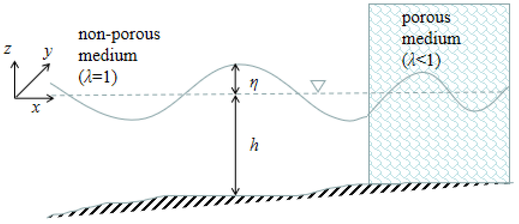
2.1. Governing Equations

Taking inertial and drag resistances into account, Vu et al. [10] have recently derived a set of Boussinesq equations for wave propagation in porous medium, which reduces to the equations of Madsen and Sørensen [25] in a non-porous medium. In their work, the equations are in non-conservative forms and are solved numerically using the FD scheme. To facilitate the use of the FV scheme, the Boussinesq equations are rewritten in the conservative form after some mathematical manipulations (see [25,30]) under the Cartesian coordinates (Figure 1).
η t + P x + Q y = 0
β P t + β x ( P 2 d ) + β y ( P Q d ) + g d η x + ψ x = 0
β Q t + β y ( Q 2 d ) + β x ( P Q d ) + g d η y + ψ y = 0
with
ψ x = β ( ( B + 1 3 ) h 2 ( P x x t + Q x y t ) h h x ( 1 3 P x t + 1 6 Q y t ) h h y 1 6 Q x t 1 6 h h x x P t 1 6 h h x y Q t + 1 3 h x 2 P t + 1 3 h x h y Q t ) B g h 3 ( η x x x + η x y y ) h h x ( 2 B g h η x x + B g h η y y ) h h y ( B g h η x y ) h h x x B g h η x h h x y B g h η y + α ( P ( B + 1 3 ) h 2 ( P x x + Q x y ) h h x ( 1 3 P x + 1 6 Q y ) h h y 1 6 Q x 1 6 h h x x P 1 6 h h x y Q + 1 3 h x 2 P + 1 3 h x h y Q )
ψ y = β ( ( B + 1 3 ) h 2 ( Q y y t + P x y t ) h h y ( 1 3 Q y t + 1 6 P x t ) h h x 1 6 P y t 1 6 h h y y Q t 1 6 h h x y P t + 1 3 h y 2 Q t + 1 3 h x h y P t ) B g h 3 ( η y y y + η x x y ) h h y ( 2 B g h η y y + B g h η x x ) h h x ( B g h η x y ) h h y y B g h η y h h x y B g h η x + α ( Q ( B + 1 3 ) h 2 ( Q y y + P x y ) h h y ( 1 3 Q y + 1 6 P x ) h h x 1 6 P y 1 6 h h y y Q 1 6 h h x y P + 1 3 h y 2 Q + 1 3 h x h y P )
where η is the free surface elevation measured from the still water level, h is the still water depth, d = h + η is the total water depth, g is the gravity acceleration, P = du and Q = dv are fluxes with u = ( u , v ) is the depth-averaged velocity vector and B = 1/15 is the dispersion parameter. β = λ + (1 − λ)(1 + κ) is the inertial resistance coefficient, with λ and κ = 0.34 being the porosity of porous medium and the added mass coefficient; α is the drag resistance coefficient calculated by
α = α l ( 1 λ λ ) 2 ν d 50 2 + α t 1 λ λ 1 d 50 2 | u |
where ν is the kinematic viscosity of water, and d50 is the size of the solid material. αl and αt are coefficients representing the laminar and turbulent flow resistances, respectively. The values of these two parameters depend on the porous material property, the Reynolds number and the flow characteristics. The universal values are not available, and we calibrate them using the experimental data (provided in Section 4) following the overwhelming majority of previous studies, e.g., [1,2,3,4,5,6,7,8,9,10].
It should be mentioned here that (i) λ = 1 and λ < 1 in Equations (1)–(3) represent wave motion in porous and non-porous mediums, respectively, which simplifies the numerical scheme, as noted before. Otherwise, additional efforts should be made to deal with the matching conditions along the interface between porous and non-porous mediums (see [9,23]); (ii) Higher-order slope terms, originally derived by Kim et al. [30], are inserted into Equations (1)–(3) to improve model performance for rapidly varying topography. (iii) B = 1/15, instead of B = 1/18 recommended in [10], is used, since they have almost indistinguishable numerical performance for the considered cases. (iv) Equations (1)–(3) are valid only for bottom-mounted and vertical porous structure. (v) Bottom friction is neglected.

2.2. Numerical Scheme and Boundary Conditions

The hybrid FV/FD shock-capturing scheme, originally proposed by the authors for wave propagation in open water [27], is adopted to solve Equations (1)–(3). These equations are almost identical to those presented in [27], except for extra terms related to porous medium, and the numerical implementation is primarily straightforward. Furthermore, the methods employed in [28] are used to deal with moving shoreline and breaking waves, which are not well addressed in [27]. The main procedures are summarized herein for clarity and completeness.
On a rectangular cell system, the convective flux terms are solved by the FV method, and the rest of the terms in the equations are discretized using the FD method. The hydrostatic construction technique is used during the implementation of the fourth-order MUSCL (Monotone Upstream-Centred Schemes for Conservation Laws) with the Minmod limiter function, which helps to capture the moving shoreline in an accurate and efficient manner [28]. A central upwind scheme is then used to calculate the interface fluxes. The third-order Runge–Kutta scheme with the adaptive time step is applied to performing time integration. The time step Δt is restricted by the Courant number Cr, which is set to 0.20 for all simulations. The velocity components are obtained by solving the tridiagonal system, resulting from discretizing the time derivative terms in Equations (2) and (3) with the second-order finite difference formula [27]. The specific values of grid size Δx will be mentioned explicitly in each test case, which are found to be sufficient to yield numerical stability and convergence for all the simulations in this study.
The unique feature of a shock-capturing Boussinesq model is its ability to capture breaking waves as discontinuities by deactivating dispersive terms. In the computation, the ratio of wave height to water depth ε (estimated approximately by η/h) and the local wave angle η are computed for each cell. If at least one of the criteria is satisfied, the corresponding cells are labeled as breaking waves and dispersive terms are deactivated. Dispersive terms can only be reactivated once ε reduces to below a certain threshold ε < 0.35. This hybrid wave breaking criteria does not need to track breaking fronts and admits the steady jumps or initial discontinuities [28].
Three ghost cells are employed to enclose the entire computational domain. For the reflective wall, the tangential and normal velocity components on ghost cells are determined from the inner domain by imposing symmetric and anti-symmetric conditions with respect to the solid wall [27]. For incident wave boundary, the variables on the ghost cells are given according to the theoretical wave solutions, i.e., solitary wave theory, linear wave theory and cnoidal wave theory in the present study, as known quantities. In this way, wave signals are sent into the computational domain to mimic wave generation from a paddle-type wavemaker. A spongey layer is also placed at the front of solid walls to absorb wave energy once necessary [14].

2.3. GPU Implementation

Boussinesq equations are phase resolving, and usually require a large number of discrete grids to obtain detailed intra-wave hydrodynamics and high resolution of coastal structures. To meet the stability requirement, the time step is usually in the order of O(T/100, where T is the typical wave period). Thus, BT simulation is computationally demanding at fine resolutions in practical applications, although it is much cheaper than RANS simulation. Recently, Fang et al. [29] successfully ported their BT model [27] to a single GPU via CUDA C. The massive computation tasks (e.g., fluxes evaluation, MUSCL reconstruction) were coded as kernel functions and executed on the GPU device. To achieve better performance, the model uses a CR (Cyclic Reduction) technique to solve massive tridiagonal linear systems and overlapped tiling/shared memory to reduce global memory access and enhance data reuse. Compared to the serial code, the maximum speedup ratios for single- and double-precision calculations are 55.56 and 32.57, respectively for tested cases. We adopt the same procedure for GPU parallel computation, further details of which can be found in [29]. High computation efficiency is another advantage of the present BT model, and to the authors’ knowledge, only a few BT models have been accelerated by the GPU technique to date [31,32,33].

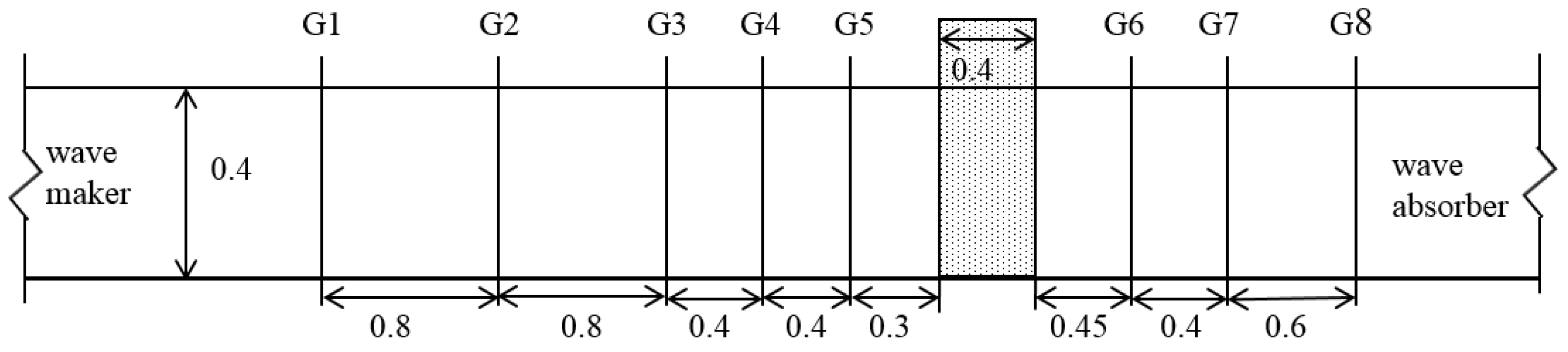
3. Physical Wave Flume Experiments

Previous laboratory datasets used to validate the BT model mainly concern solitary wave and statistical wave height of short waves, while time series of the free surface elevation of dispersive waves are less reported. New laboratory experiments are thus conducted to provide a larger dataset. Figure 2 shows the sketch of the experimental setup. The wave flume is 34.55 m long, 0.8 m wide and 1.0 m deep. A piston-type wavemaker is installed on one end of the flume and a sponge layer is placed at the other end to absorb wave energy. The water depth is kept constant and equal to 0.4 m. A 0.4 m wide and 0.64 m high porous vertical breakwater is built with a metallic mesh filled with glass spheres and positioned 22.8 m from the mean position of the wave paddle. The spheres have a diameter of 0.05 m and a porosity of 0.35. Five tests are listed in Table 1, consisting of three regular wave cases and two solitary wave cases with different water dispersions (denoted by dimensionless water depth kh, k is wave number) and nonlinearities (denoted by H/h, H is wave height). Eight capacity-type wave gauges are positioned at x = 20.1, 20.9, 21.7, 22.1, 22.5, 23.65, 24.05, 24.65 m to collect free surface elevation along the wave flume. The sampling rate is 50 Hz.

4. Results and Discussion

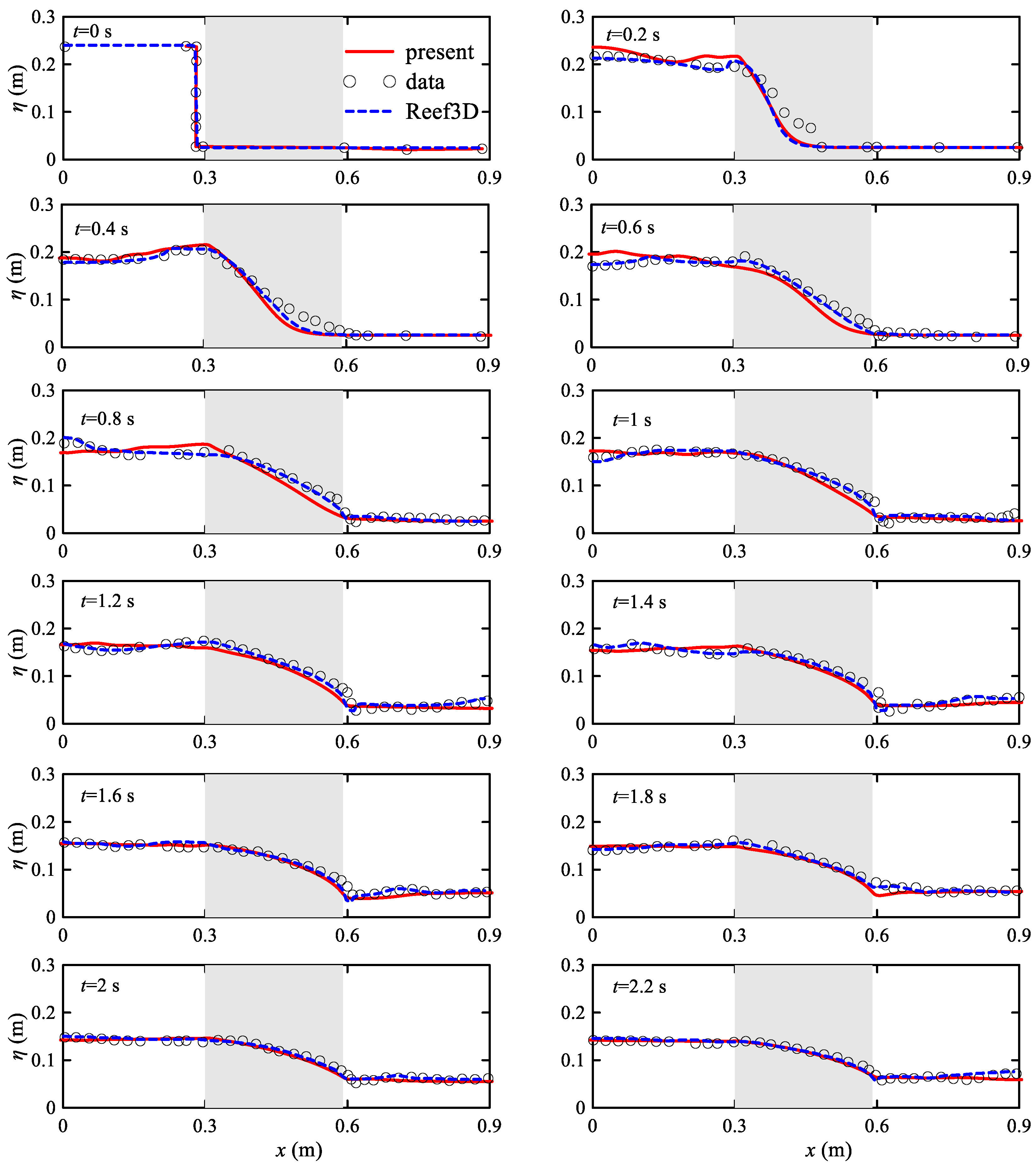
4.1. Dam Break on a Porous Structure

The first test case is to simulate the experiments of dam break on a porous structure conducted by Liu et al. [1]. The water tank used in the experiments is 0.892 m long, 0.44 m wide, and 0.58 m high. Crushed rocks with a mean diameter of d50 = 0.0159 m and porosity λ = 0.49 were placed in the center of the water tank to form a 0.29 m long and 0.58 m tall dam. The reservoir has an initial water height of 0.25 m and is separated from the porous dam by a 0.02 m thick gate. The numerical setup is the same as the experimental setup and is illustrated in the first panel of Figure 3, which corresponds to the initial state at t = 0 s. The simulation domain is discretized into cells of Δx = 0.005 m. The drag coefficients of αl = 4000, αt = 4.2 are calibrated by running trial-and-error simulations to achieve the best agreement between numerical results and experimental data.
To evaluate the agreements between numerical results and experimental data for a given quantity v, the Willmott index [34] is used. This index is introduced as
W v = 1 j = 1 n [ y ( j ) x ( j ) ] 2 j = 1 n [ | y ( j ) x ¯ | + | x ( j ) x ¯ | ] 2
where x(j) is the measured data point, y(j) is the computation result, and x ¯ is the mean value of series y(j). Perfect agreement is indicated by W = 1, whereas W = 0 indicates complete disagreement.
Figure 3 compares the simulated water level with the experimental data. The overall processes such as upward jet as the water body crashes into the porous medium (t = 0.2 s), the reflection of dam break flow from the right end of water tank (t = 1.4~1.8 s) and the trend of water seeping porous structure are reasonably predicted by the BT model. It is noted that water close to the bottom moves earlier than the water at the free surface when the gate is opened manually in the experiments. However, the depth-integrated BT model cannot reproduce this process and leads to significant inconsistencies with the measurements at t = 0.2, 0.4, 0.6 and 0.8 s. Better agreements are achieved as the flow evolves (t = 1.0–2.2 s). The RANS simulation results using REEF3D in [4] are also shown in Figure 3 as a comparison. The mean value of the Willmott index from the present simulation and RANS simulation are 0.953 and 0.962, respectively. RANS simulations present better predictions, as expected, except for the disagreements at the initial stage due to the reasons mentioned above. After t = 0.8 s, the simulation results of the present BT model are comparable to the predictions of RANS simulations. BT models based on the FD method fail to simulate this test case, since they are unable to treat the water discontinuity at t = 0 s, which demonstrates the merits of the shock-capturing hybrid scheme adopted in the present study.

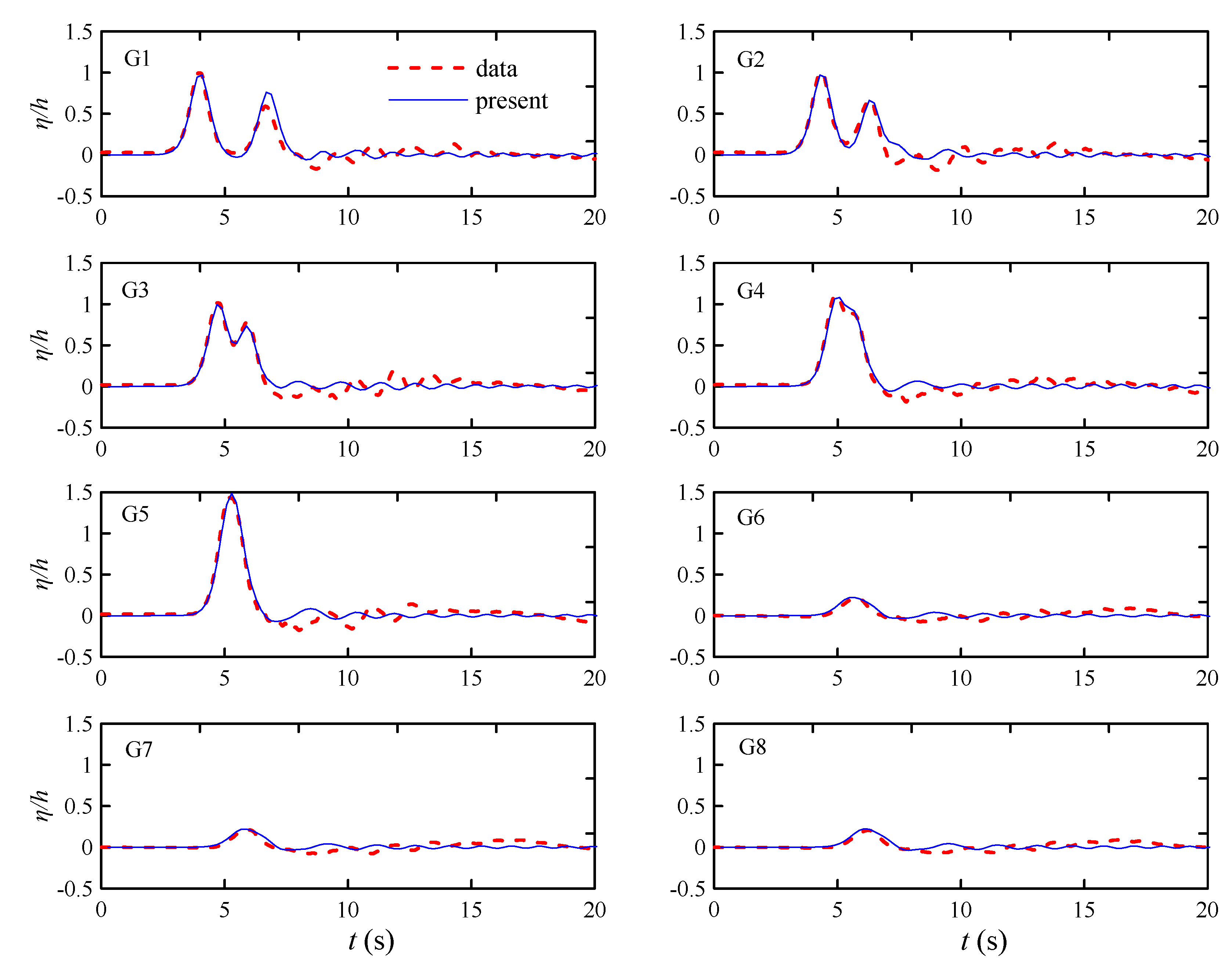
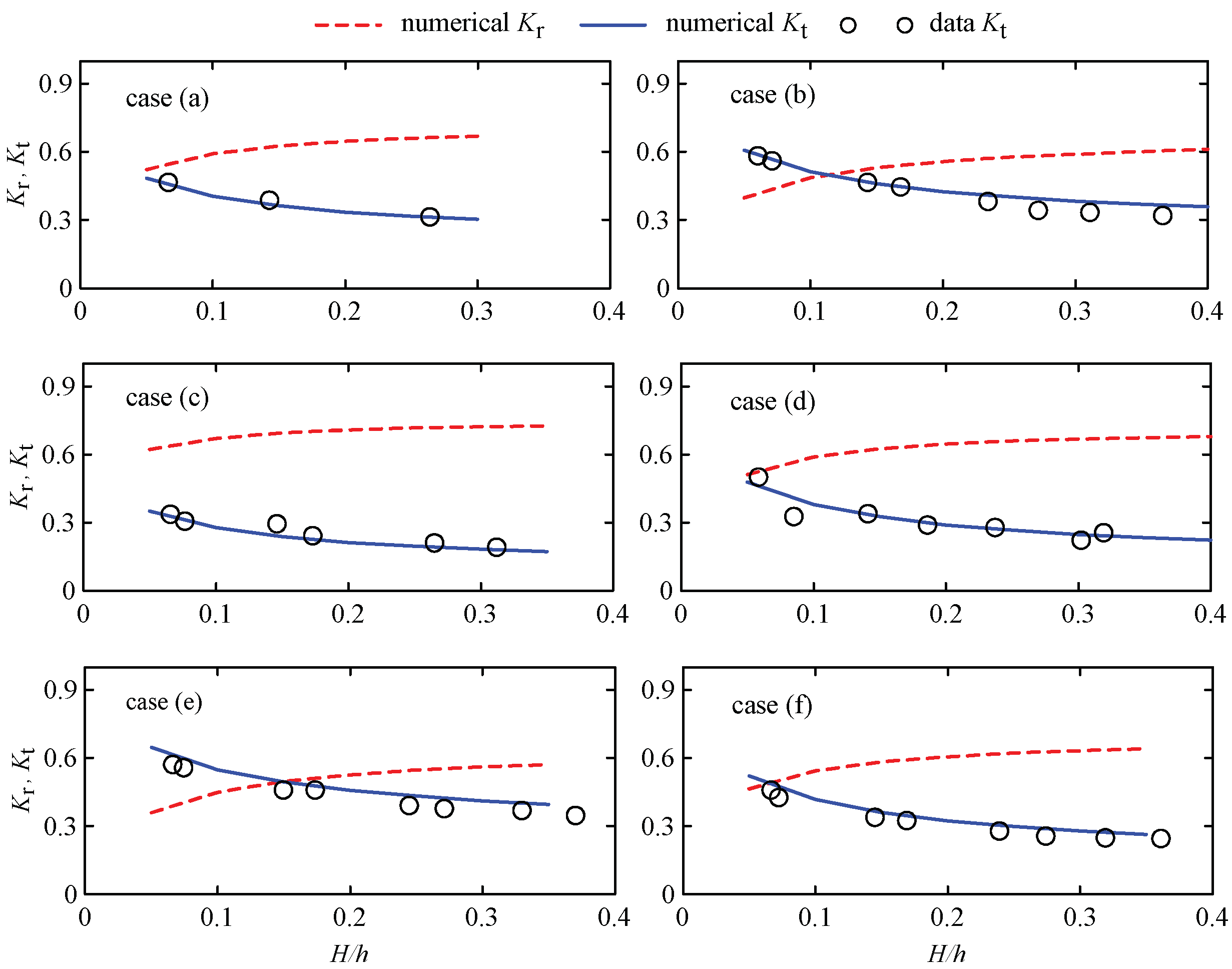
4.2. Solitary Wave Passing through Porous Breakwaters

Two cases from the new experiments (S1 and S2 in Table 1) are first simulated to show the model performance in terms of solitary wave interaction with porous structure. The numerical flume is the same as the physical flume shown in Figure 2. The grid size is 0.01687 m, and αl = 800, αt = 9.0. A 3.0 m-wide sponger layer is placed at the end of the numerical flume to absorb wave energy.
Figure 4 and Figure 5 show the comparison of the computed free surface elevation with the experiment data, respectively. For case S1, the wave gauges located in front of the porous structure (G1–G3) clearly record two peaks, corresponding to the incident and reflected waves from the porous structure. The BT model captures the arrival time of both reflected and transmitted waves, but it overestimates the amplitude of the secondary wave at G1 and G2. Adjacent to the porous wall at G5, these two peaks merge into one with a large amplitude, about 1.5 times that of the incident amplitude. The solitary wave shape is well maintained on the leeside of the breakwater at G6–G8, where the wave amplitude is largely dissipated by 71% due to the presence of porous breakwater. Case S2 is more nonlinear than Case S1, but a similar evolution process is observed. For this case, the dimensionless transmission amplitude is reduced to 0.21, which is inconsistent with previous findings that large nonlinearity causes a smaller transmission coefficient [23,35]. In summary, the waveform and phase are predicted very well for both cases.
Regarding a solitary wave passing through porous structures, previous studies in the literature mainly concerned with the transmitted and reflected wave amplitude. We further simulate six cases from the experiments of Vidal et al. [35], where transmission and reflection coefficients are available and have been extensively used for model validation. Table 2 summarizes the material property and dimension of porous breakwaters from the experiments. In the simulation, a grid size of 0.025 m is used, and the drag coefficients are set to αl = 800, αt = 3.0. Figure 6 compares the transmission coefficients Kt from the current simulation with the experimental data, and they are in good agreement. The reflection coefficients Kr are also plotted in the figure. As nonlinearity increases, the decreasing trend of Kt and the increasing trend of Kr are well predicted by the BT simulation.

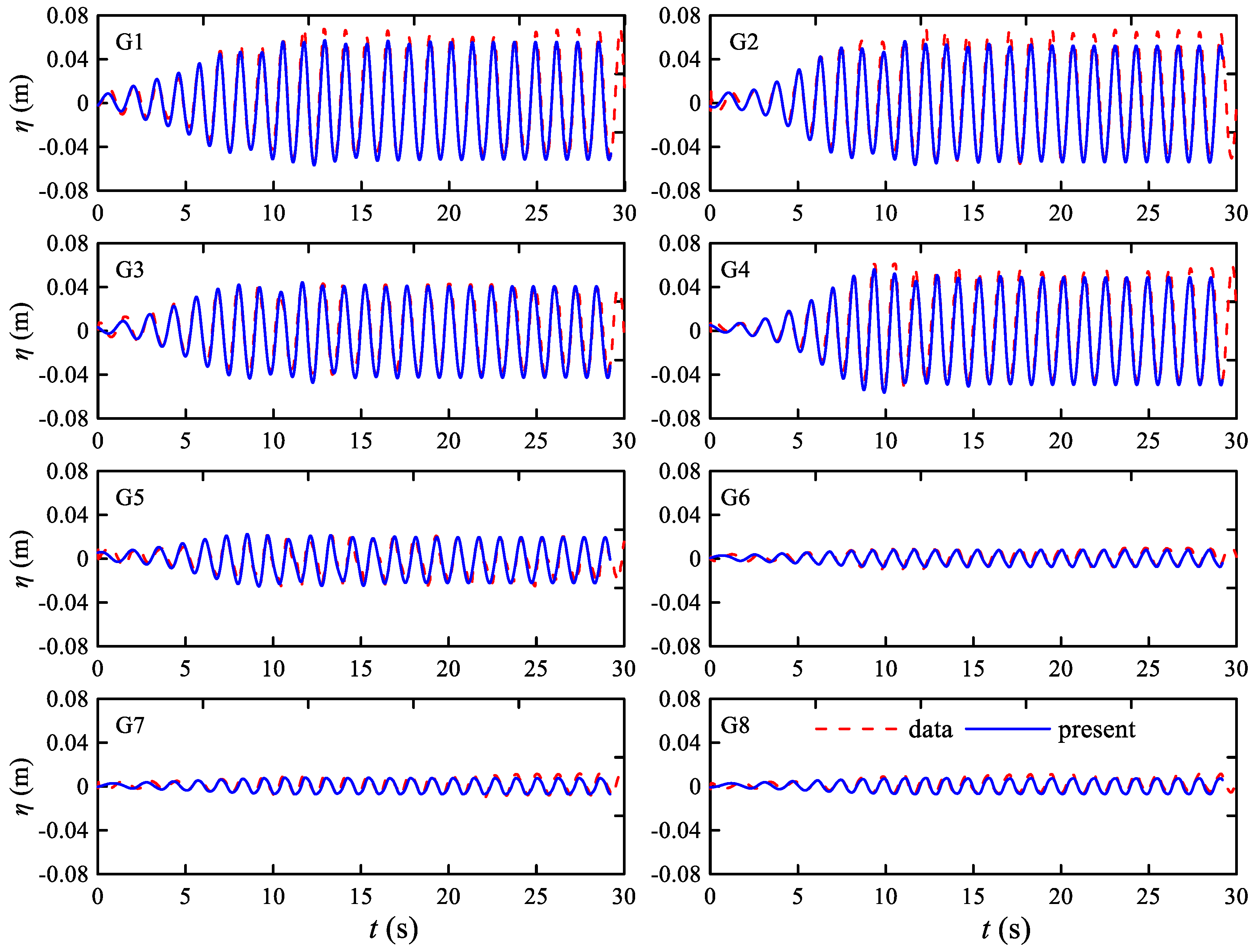
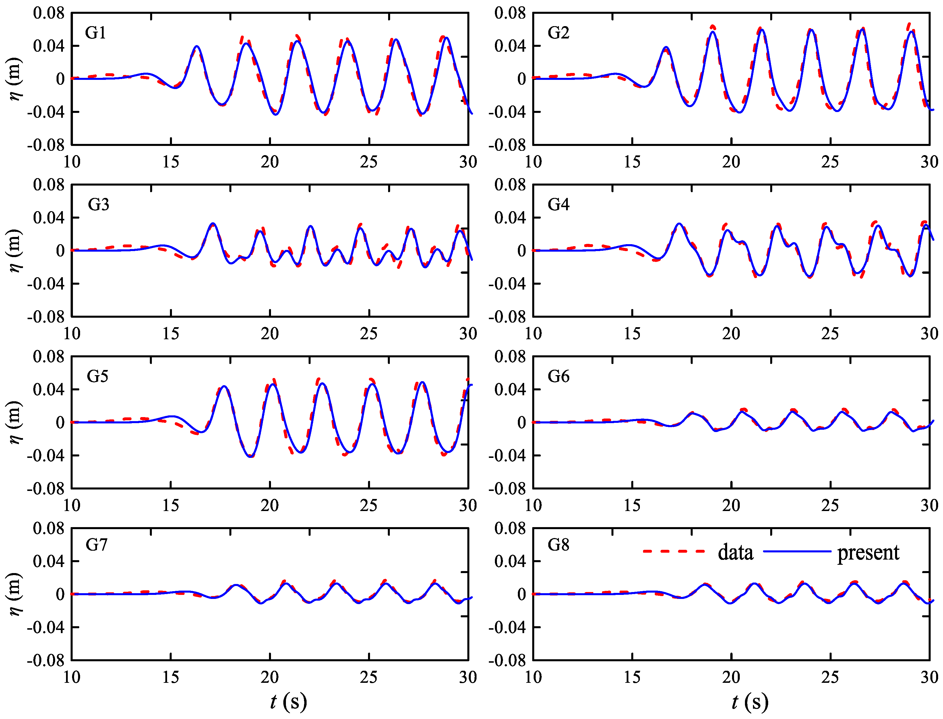
4.3. Regular Wave Passing through Porous Breakwaters

In this section, numerical simulations are conducted for regular wave cases (R1–R3 in Table 1) to test the model’s ability to describe short dispersive wave interaction with porous structures. A grid size of Δx = 0.02 m is used to discretize the computational domain. A 3.0 m-wide sponger layer is placed at the end of the numerical flume to absorb wave energy.
Figure 7, Figure 8 and Figure 9 compare the time series of computed and measured free surface elevation at eight wave gauge locations, five in front of the porous structure and three leeward of the breakwater. For all cases, both the wave shape and phase are reproduced by the BT model with a high degree of accuracy. The incident waves are partially reflected from the porous structure, which interacts with the incident waves and creates a standing wave pattern in front of the structure (G1–G5). These wave profiles are very well caught during the simulation, including the initial state and the subsequent quasi-steady wave pattern. On the leeward side of the porous breakwater, the wave profiles calculated at locations G6–G8 correspond to the incident wave that is damped by the porous structure. The wave shape and phase are also predicted very well by the BT model for three cases. The mean values of the Willmott index from the present simulation are 0.972 (Case R1), 0.982 (Case R2) and 0.946 (Case R3), showing reasonable prediction accuracy.

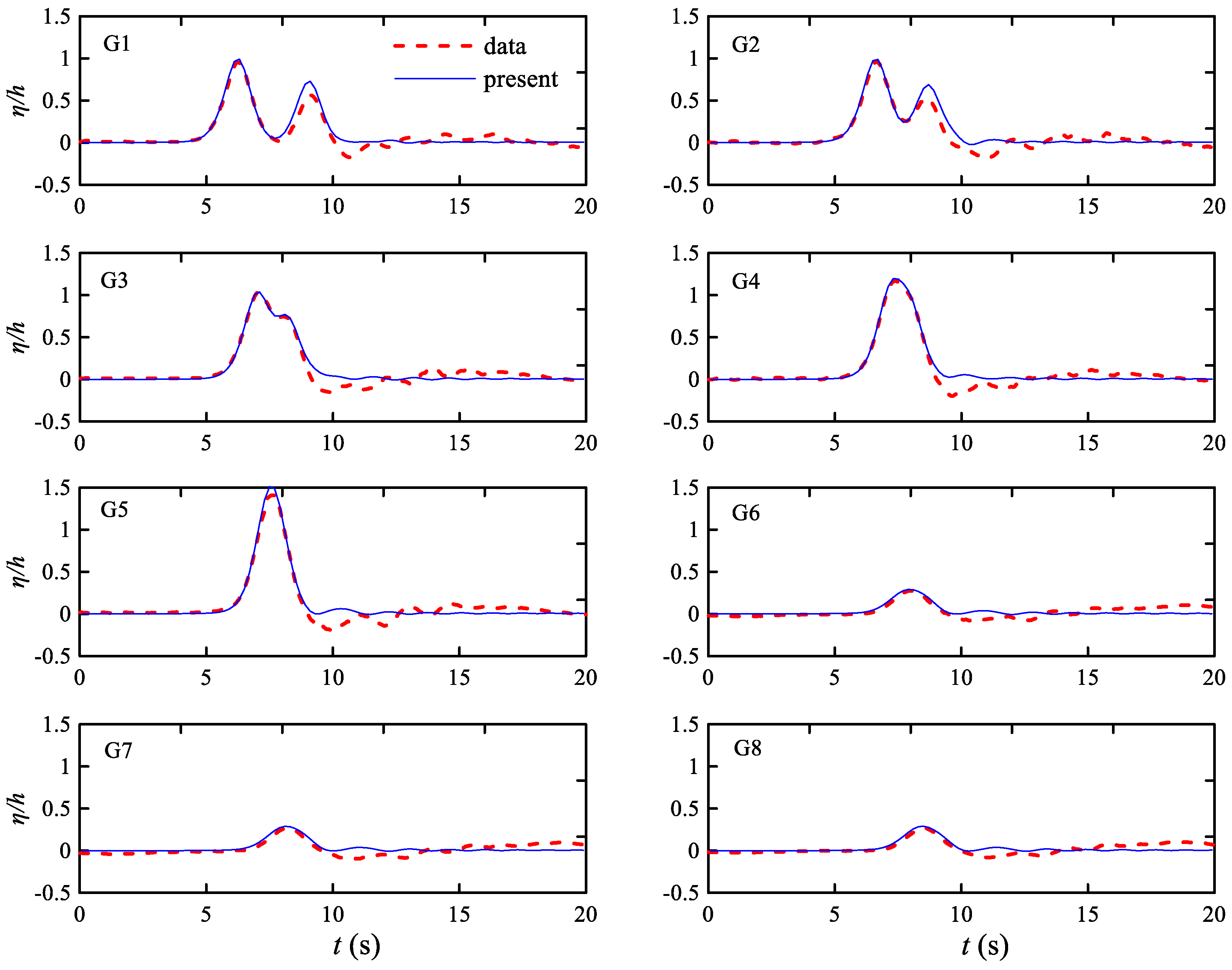
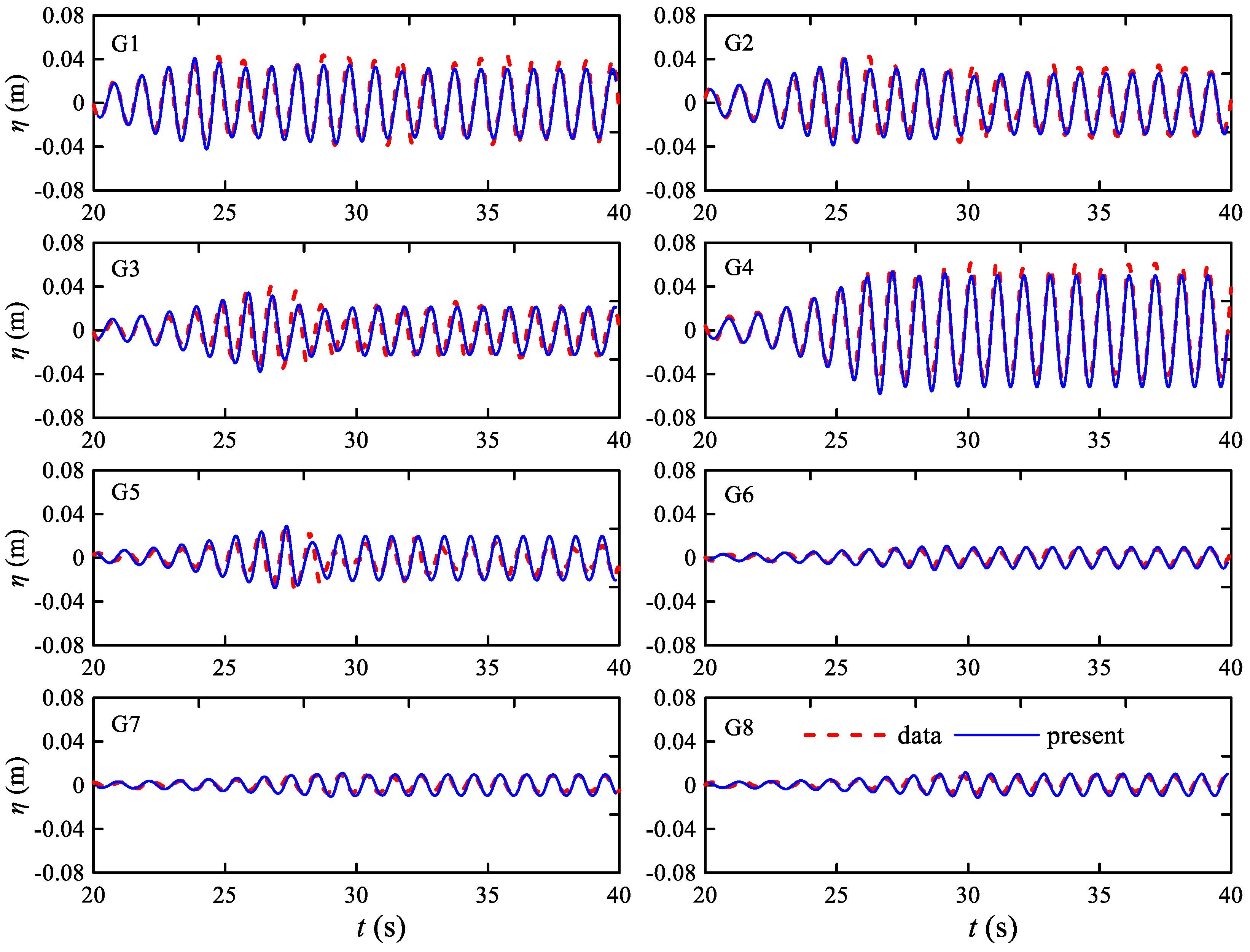
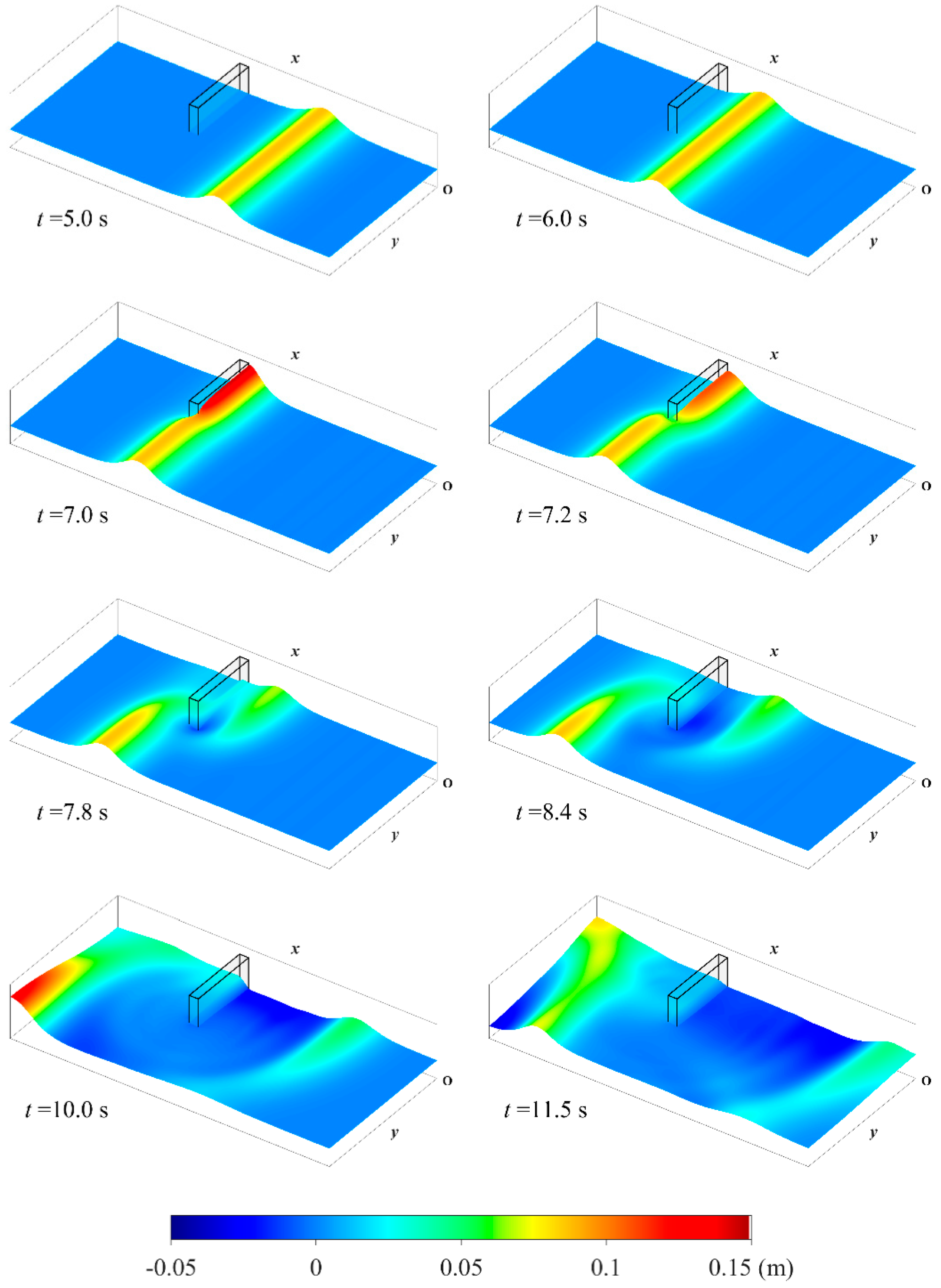
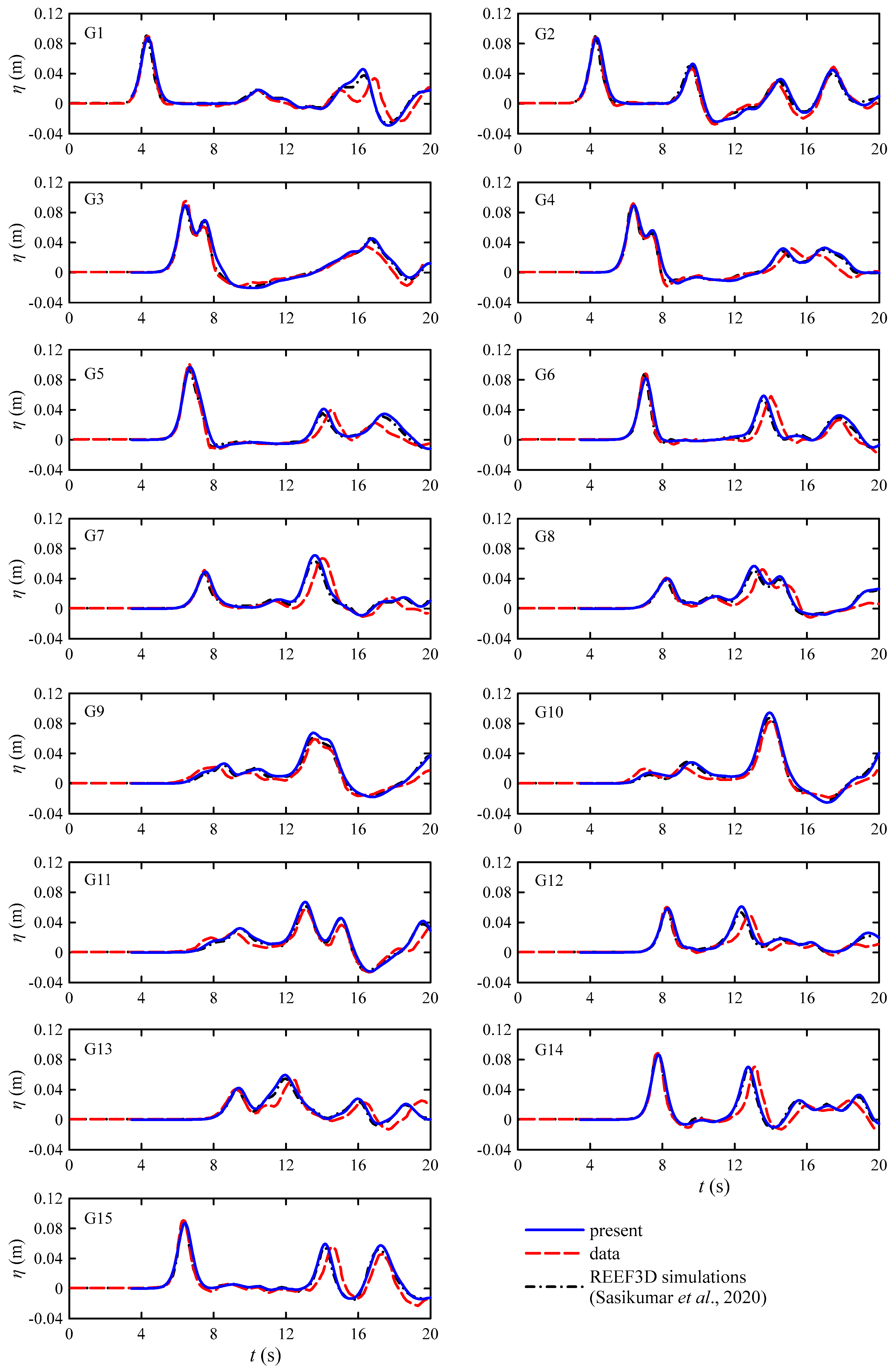
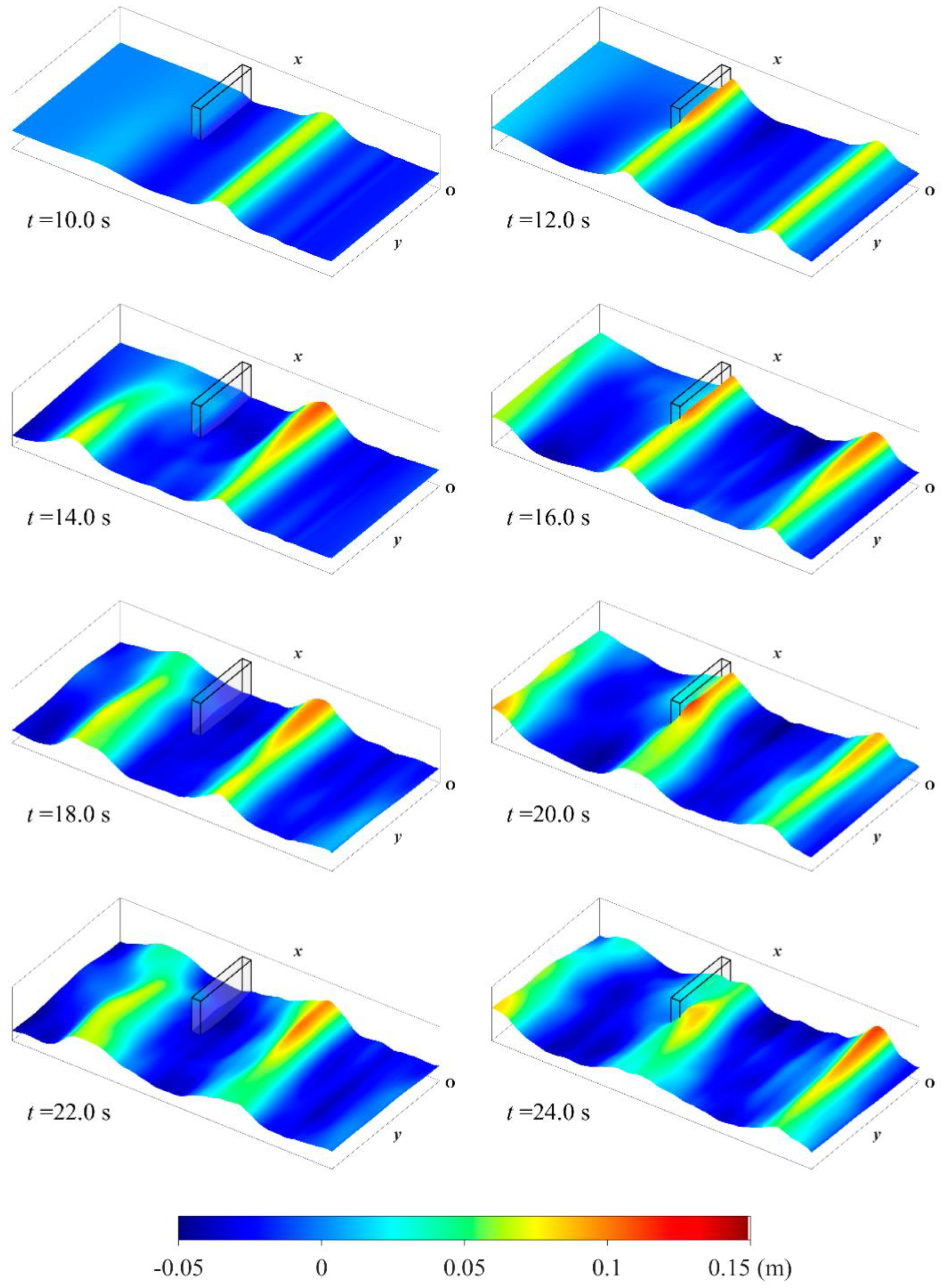
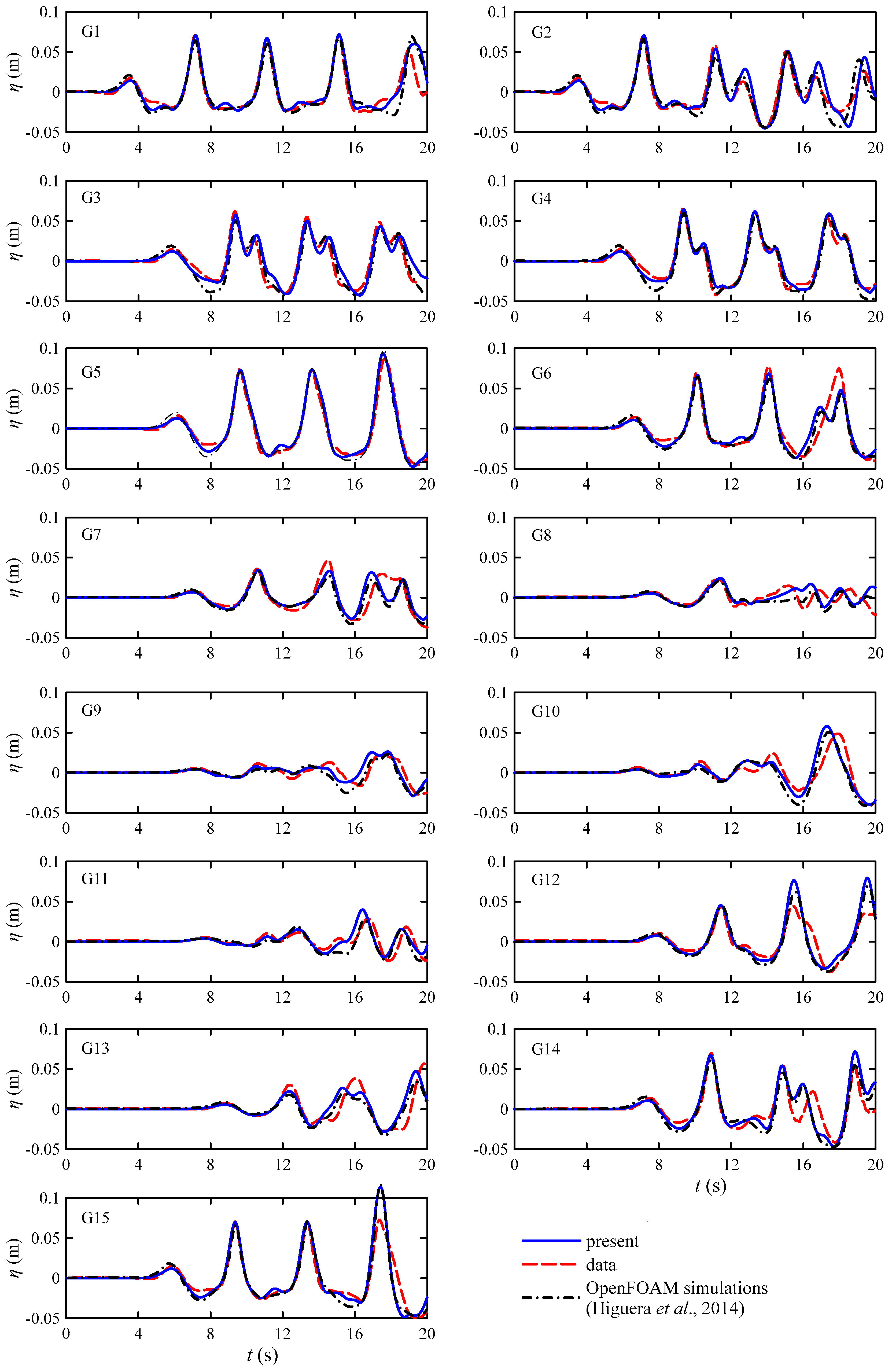
4.4. Wave Passing through Porous Breakwater in a Wave Basin

In order to examine the model performance for three-dimensional problems, numerical results are compared with the experimental measurements conducted by Lara et al. [36] in a wave basin. The sketch of the experiments and 15 wave gauges are shown in Figure 10. Table 3 lists the locations of 15 wave gauges. The wave basin is 18.2 m long, 8.6 m wide and 1.0 m high. A porous breakwater 4.0 m long, 0.50 m wide and 0.6 m high is built with the porous materials with λ = 0.51 and d50 = 1.5 cm. The breakwater is placed perpendicular to the direction of wave propagation at a distance of 10.5 m from the wavemaker. The water depth is kept constant and equal to 0.4 m. Two wave conditions have been selected for simulation. First, a solitary wave of 9 cm in height is tested (H/h = 0.225). Then, cnoidal waves with H = 9 cm and T = 4 are generated. The computational domain is discretized with a grid size of Δx = 0.05 m and Δy = 0.0336 m. The values of the drag coefficients are αl = 800 and αt = 3. As in the experiments, the two lateral sides and the right end of the wave basin are treated as solid walls in the simulation.
The simulated interaction processes between solitary wave and porous structure are presented in Figure 11. As can be seen from this figure, wave damping and wave transmission resulting from wave penetration through the porous structure, wave reflection from porous structure and side walls, wave diffraction and wave run-up on structure result in a complicated wave field. The solitary wave is approaching the porous structure at t = 5.0 s and t = 6.0 s. The incident wavefront is separated by the structure and the transmitted wave in the unblocked region, as seen at t = 7.0 s. The solitary wave climbs up the structure at the same time, and the subsequent run down is observed at t = 7.25 s. The panels corresponding to t = 7.85 s and t = 8.45 s show the wave transmitted through and beyond the structure approaching the end of the wave basin and the first partially reflected wave from the structure traveling toward the wavemaker. The end wall of the wave basin reflects the waves, and these waves propagate towards the structure at t = 10.0 s and t = 11.5 s. The second time wave interaction will occur subsequently (not shown in Figure 11).
A further comparison of the time series of free surface elevation at 15 wave gauges with experimental data is presented along with the RANS type simulation using REEF3D [4] in Figure 12. The incident wave and the reflected wave from the end of the wave basin can be seen at G1. G2 records the incident wave, the partially reflected wave from the porous structure and the reflected wave from the end of the wave basin in sequence. Both G3 and G4 record a secondary crest, as they are positioned just 1.0 m from the porous structure and are quickly affected by wave reflection. G5 and G6 are located around the head of the porous structure and have a similar variation trend. Wave gauges G7–G11 and G13 are placed on the leeside of the porous structure. The amplitude of the transmitted wave at these locations is greatly damped by the porous structure. In contrast, the second peak formed by the reflected wave from the end of the domain has a relatively larger amplitude. G12 is located further behind the structure head and the incident wave consists of the unaffected part of the wave and the part transmitted through the structure. It also records the reflected waves from the basin wall. G14 and G15 are fully exposed to the incident wave and are less affected by the porous structure. The current BT simulations agree well with the experimental data, with the deviations mainly observed in the phase of the reflected waves. This lag is attributed to discrepancies in several measurements, including the breakwater geometry, its installation location in the basin and slight variations in the wave gauge locations [36]. The developed BT model shows a high degree of accuracy in predicting the free surface time series with the mean value of W = 0.949, achieving almost identical performance to that of REEF3D (W = 0.952).
The simulated three-dimensional wave field for the cnoidal wave case is plotted in Figure 13. Figure 14 compares the time series of simulated free surface elevation with the laboratory measurements and the OpenFOAM simulations [3]. Unlike the previous isolated solitary wave case, cnoidal waves are sent into the wave basin continuously. Wave reflections from porous structures and three sidewalls, the interaction of incident and reflected waves and the interaction between these waves and porous structure are thus more complicated. Overall, the BT model captures the wave shape and amplitude at all wave gauge locations with reasonable accuracy, although less satisfactory results are observed towards the end of the simulation. The capability of the BT model to predict three-dimensional dispersive problems is proved. The mean value of the Willmott index from the present simulation and RANS simulation are 0.902 and 0.906, respectively, for this case, illustrating almost equivalent performance. It is reported that 20 s are simulated in less than 17 h using 128 processors (2.6 GHz) for OpenFOAM simulations [3]. It only takes 5.3 min using two processors (3.6 GHz) with the aid of NVIDIA GeForce GTX 970 card for the present BT simulation.

5. Conclusions

A set of extended Boussinesq equations [10] is numerically solved using a hybrid FV/FD scheme proposed by the authors [27,29] to simulate wave propagation through coastal porous structures. The present work is also regarded as a functional extension of our previous BT model developed for open-water problems [27], since the equations are roughly the same. A wide range of numerical simulations are carried out to test the capability of the Boussinesq equations, as well as the adopted numerical scheme. To this end, new experiments for solitary wave and regular wave interaction with a porous wall are also conducted in a wave flume.
The simulation of dam break flow in a porous abutment shows the merit of the proposed shock-capturing scheme. BT models based on the FD method do not resolve the initial discontinuity state, let alone the subsequent evolution process. A series of vertical two-dimensional and horizontal two-dimensional test cases for solitary wave and regular wave are further simulated. The computed results are found to be in generally good agreement with the experimental data, even compared with the RANS type simulation results in the literature. We thus conclude that the developed BT model is capable of handling wave interaction with porous structures in the coastal region for a wide range of scenarios after careful calibration of the porosity-related coefficients. GPU parallel computation further reduces the computation time greatly and enhances model capabilities in practical applications.

Author Contributions

Conceptualization, K.F. and M.H.; methodology, K.F. and M.H.; software, G.C. and J.W.; validation, K.F., M.H., G.C., J.W. and H.W.; formal analysis, K.F., M.H., G.C., J.W. and H.W.; investigation, H.W.; resources, H.W. and T.J.; data curation, T.J.; writing—original draft preparation, K.F. and M.H.; writing—review and editing, K.F., M.H., G.C., H.W. and T.J.; visualization, G.C. and J.W.; supervision, K.F. and M.H.; project administration, K.F.; funding acquisition, K.F. All authors have read and agreed to the published version of the manuscript.

Funding

This research was funded by the National Key Research and Development Program under contract No. 2019YFC1407700, National Natural Science Foundation of China under contract Nos. 52071057, 52171247, 51579034, 51779022 and 51809053, and Open Research Project of the National Key Laboratory of Environmental Protection and Marine Ecological Environment Restoration under contract No. 202108.

Institutional Review Board Statement

Not applicable.

Informed Consent Statement

Not applicable.

Conflicts of Interest

The authors declare no conflict of interest.

References

  1. Liu, P.L.F.; Lin, P.; Chang, K.A.; Sakakiyama, T. Numerical modeling of wave interaction with porous structures. J. Waterw. Port Coast. Ocean Eng. 1999, 125, 322–330. [Google Scholar] [CrossRef]
  2. Cheng, Y.Z.; Jiang, C.B.; Wang, Y.Y. A coupled numerical model of wave interaction with porous medium. Ocean Eng. 2009, 36, 952–959. [Google Scholar] [CrossRef]
  3. Higuera, P.; Lara, J.L.; Losada, I.J. Three-dimensional interaction of waves and porous coastal structures using OpenFOAM®. Part I: Formulation and validation. Coast. Eng. 2014, 83, 243–258. [Google Scholar] [CrossRef]
  4. Sasikumar, A.; Kamath, A.; Bihs, H. Modeling porous coastal structures using a level set method based VRANS-solver on staggered grids. Coast. Eng. J. 2020, 62, 198–216. [Google Scholar] [CrossRef]
  5. Cea, L.; Vázquez-Cendón, E. Unstructured finite volume discretization of two-dimensional depth-averaged shallow water equations with porosity. Int. J. Numer. Methods Fluids 2010, 63, 903–930. [Google Scholar] [CrossRef]
  6. Mohamed, K. A finite volume method for numerical simulation of shallow water models with porosity. Comput. Fluids 2014, 104, 9–19. [Google Scholar] [CrossRef]
  7. Abbott, M.B.; Petersen, H.M.; Skovgaard, O. On the numerical modelling of short waves in shallow water. J. Hydraul. Res. 1978, 16, 173–204. [Google Scholar] [CrossRef]
  8. Madsen, P.A.; Warren, I.R. Performance of a numerical short-wave model. Coast. Eng. 1984, 8, 73–93. [Google Scholar] [CrossRef]
  9. Liu, P.L.F.; Wen, J. Nonlinear diffusive surface waves in porous media. J. Fluid Mech. 1997, 347, 119–139. [Google Scholar] [CrossRef]
  10. Vu, V.N.; Lee, C.; Jung, T.H. Extended Boussinesq equations for waves in porous media. Coast. Eng. 2018, 139, 85–97. [Google Scholar] [CrossRef]
  11. Shao, S. Incompressible SPH flow model for wave interactions with porous media. Coast. Eng. 2010, 57, 304–316. [Google Scholar] [CrossRef]
  12. Akbari, H.; Namin, M.M. Moving particle method for modeling wave interaction with porous structures. Coast. Eng. 2013, 74, 59–73. [Google Scholar] [CrossRef]
  13. Ren, B.; Wen, H.; Dong, P.; Wang, Y. Improved SPH simulation of wave motions and turbulent flows through porous media. Coast. Eng. 2016, 107, 14–27. [Google Scholar] [CrossRef]
  14. MIKE Powered by DHI. Available online: https://www.mikepoweredbydhi.com (accessed on 9 December 2021).
  15. Kirby, J.T.; Wei, G.; Chen, Q.; Kennedy, A.; Dalrymple, R.A. FUNWAVE 1.0 Fully Nonlinear Boussinesq Wave Model Documentation and User’s Manual; University of Delaware: Newwark, NJ, USA, 1998. [Google Scholar]
  16. Lynett, P.J. A Multi-Layer Approach to Modeling Generation, Propagation, and Interaction of Water Waves. Ph.D. Thesis, Cornell University, Ithaca, NY, USA, 2002. [Google Scholar]
  17. Cruz, E.C.; Isobe, M.; Watanabe, A. Boussinesq equations for wave transformation on porous beds. Coast. Eng. 1997, 30, 125–156. [Google Scholar] [CrossRef]
  18. Hsiao, S.C.; Liu, P.L.F.; Chen, Y. Nonlinear water waves propagating over a permeable bed. In Proceedings of the Mathematical, Physical and Engineering Sciences of the Conference, Ithaca, NY, USA, 8 June 2002; pp. 1291–1322. [Google Scholar]
  19. Cruz, E.C.; Chen, Q. Numerical modeling of nonlinear water waves over heterogeneous porous beds. Ocean Eng. 2007, 34, 1303–1321. [Google Scholar] [CrossRef]
  20. Hsiao, S.C.; Hu, K.C.; Hwung, H.H. Extended Boussinesq equations for water-wave propagation in porous media. J. Eng. Mech. 2010, 136, 625–640. [Google Scholar] [CrossRef]
  21. Peregrine, D.H. Long waves on a beach. J. Fluid Mech. 1967, 27, 815–827. [Google Scholar] [CrossRef]
  22. Madsen, P.A. Wave reflection from a vertical permeable wave absorber. Coast. Eng. 1983, 7, 381–396. [Google Scholar] [CrossRef]
  23. Lynett, P.; Liu, P.; Losada, I.; Vidal, C. Solitary wave interaction with porous breakwaters. J. Waterw. Port. Coast. Ocean Eng. 2000, 126, 314–322. [Google Scholar] [CrossRef]
  24. Wu, T.Y. Long Waves in ocean and coastal waters. J. Eng. Mech. 1981, 107, 501–522. [Google Scholar] [CrossRef]
  25. Madsen, P.A.; Sørensen, S.R. A new form of the Boussinesq equations with improved linear dispersion characteristics. Part 2. A slowly-varying bathymetry. Coast. Eng. 1992, 18, 183–204. [Google Scholar] [CrossRef]
  26. Shi, F.; Kirby, J.T.; Harris, J.C.; Geiman, J.D.; Grilli, S.T. A high-order adaptive time-stepping TVD solver for Boussinesq modeling of breaking waves and coastal inundation. Ocean Model 2012, 43–44, 36–51. [Google Scholar] [CrossRef]
  27. Fang, K.; Zou, Z.; Dong, P.; Liu, Z.; Gui, Q.; Yin, J. An efficient shock capturing algorithm to the extended Boussinesq wave equations. Appl. Ocean Res. 2013, 43, 11–20. [Google Scholar] [CrossRef]
  28. Fang, K.; Liu, Z.; Zou, Z. Fully Nonlinear Modeling Wave Transformation over Fringing Reefs Using Shock-Capturing Boussinesq Model. J. Coast. Res. 2016, 32, 164–171. [Google Scholar] [CrossRef]
  29. Fang, K.; Sun, J.; Song, G.; Wang, G.; Wu, H.; Liu, Z. A GPU accelerated Boussinesq-type model for coastal waves. Acta Oceanol. Sin. 2022, 41, 1–11. [Google Scholar] [CrossRef]
  30. Kim, G.; Lee, C.; Suh, K.D. Extended Boussinesq equations for rapidly varying topography. Ocean Eng. 2009, 36, 842–851. [Google Scholar] [CrossRef]
  31. Yuan, Y.; Shi, F.; Kirby, J.T.; Yu, F. FUNWAVE-GPU: Multiple-GPU acceleration of a Boussinesq-type wave model. J. Adv. Model Earth Sys. 2020, 12, e2019MS001957. [Google Scholar] [CrossRef]
  32. Tavakkol, S.; Lynett, P. Celeris: A GPU-accelerated open source software with a Boussinesq-type wave solver for real-time interactive simulation. Comput. Phys. Commun. 2017, 217, 117–127. [Google Scholar] [CrossRef]
  33. Kim, B.; Oh, C.; Yi, Y.; Kim, D.H. GPU-Accelerated Boussinesq Model Using Compute Unified Device Architecture FORTRAN. J. Coast. Res. 2018, 85, 1176–1180. [Google Scholar] [CrossRef]
  34. Willmott, C.J. On the validation of models. Phys. Geogr. 1981, 2, 184–194. [Google Scholar] [CrossRef]
  35. Vidal, C.; Losada, M.A.; Medina, R.; Rubio, J. Solitary wave transmission through porous breakwaves. In Proceedings of the 21st International Conference on Coastal Engineering, Torremolinos, Spain, 29 January 1988. [Google Scholar]
  36. Lara, J.L.; del Jesus, M.; Losada, I.J. Three-dimensional interaction of waves and porous coastal structures: Part II: Experimental validation. Coast. Eng. 2012, 64, 26–46. [Google Scholar] [CrossRef]
Figure 1. Sketch of wave propagation in porous media.
Jmse 10 01367 g001
Figure 2. The sketch of experimental setup and wave gauge locations. (All dimensions in meters).
Jmse 10 01367 g002
Figure 3. Comparison of water level from the BT model simulation, experimental data and REEF3D simulation [4] (dashed line).
Jmse 10 01367 g003
Figure 4. Comparison of free surface elevation between present simulation (solid line) and experimental data (dashed line) for Case S1 (H/h = 0.12).
Jmse 10 01367 g004
Figure 5. Comparison of free surface elevation between present simulation (solid line) and experimental data (dashed line) for Case S2 (H/h = 0.22).
Jmse 10 01367 g005
Figure 6. Reflection and transmission coefficients versus wave nonlinearity for solitary waves passing through porous breakwater of Vidal et al.’s experiments [36].
Jmse 10 01367 g006
Figure 7. Time series of surface elevation for regular wave propagation in porous structure (Case R1).
Jmse 10 01367 g007
Figure 8. Time series of surface elevation for regular wave propagation in porous structure (Case R2).
Jmse 10 01367 g008
Figure 9. Time series of surface elevation for regular wave propagation in porous structure (Case R3).
Jmse 10 01367 g009
Figure 10. Setup of breakwater and wave gauges of Lara et al.’s experiments [36].
Jmse 10 01367 g010
Figure 11. Free surface elevation at different instants for solitary wave interaction with a porous structure (wave propagates from right to left in each subfigure).
Jmse 10 01367 g011
Figure 12. Time series of surface elevation for solitary wave propagation through porous breakwater [4].
Jmse 10 01367 g012
Figure 13. Free surface elevation at different instants for cnoidal wave interaction with a porous structure (wave propagates from right to left in each subfigure).
Jmse 10 01367 g013
Figure 14. Time series of surface elevation for cnoidal wave propagation through porous breakwater [3].
Jmse 10 01367 g014
Table 1. Test cases in flume experiments.
Case No.Wave TypeH (m)T (s)h (m)khH/h
R1Regular wave0.0721.00.51.720.18
R2Regular wave0.0721.20.41.300.18
R3Regular wave0.0762.50.40.530.19
S1Solitary wave0.046-0.4-0.12
S2Solitary wave0.086-0.4-0.22
Table 2. Test cases of Vidal et al.’s experiments [35].
Caseh (cm)H/hStructure Width (cm)d50 (cm)λ
(a)30.00.06–0.26201.430.44
(b)30.20.06–0.23202.430.44
(c)30.00.07–0.27401.430.44
(d)31.70.06–0.24402.430.44
(e)30.10.07–0.33203.150.42
(f)30.10.07–0.32403.150.42
Table 3. Locations of wave gauges.
Gauge No.x (m)y (m)Gauge No.x (m)y (m)
115.07.0922.01.5
215.01.01021.50.5
319.51.01123.00.5
419.53.01223.54.0
520.04.01325.02.0
621.04.51422.57.0
721.53.51519.57.5
822.52.5
Publisher’s Note: MDPI stays neutral with regard to jurisdictional claims in published maps and institutional affiliations.

