

Effects of Tidal Stream Energy Exploitation on Estuarine Circulation and Its Seasonal Variability
 , ,
, ,  and
and
Abstract
:1. Introduction
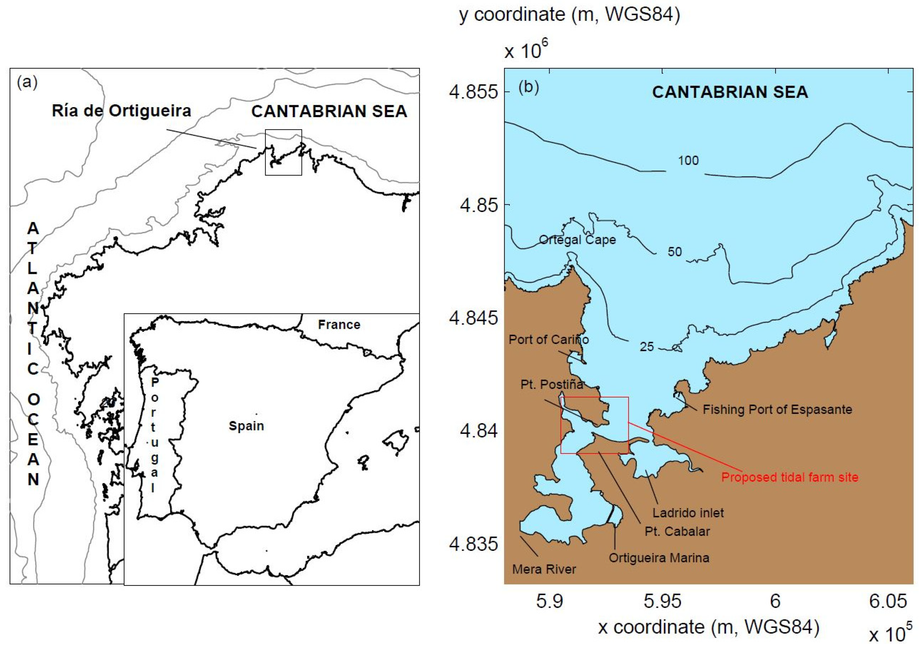
2. Study Area
3. Materials and Methods
3.1. Numerical Model (I): Equations
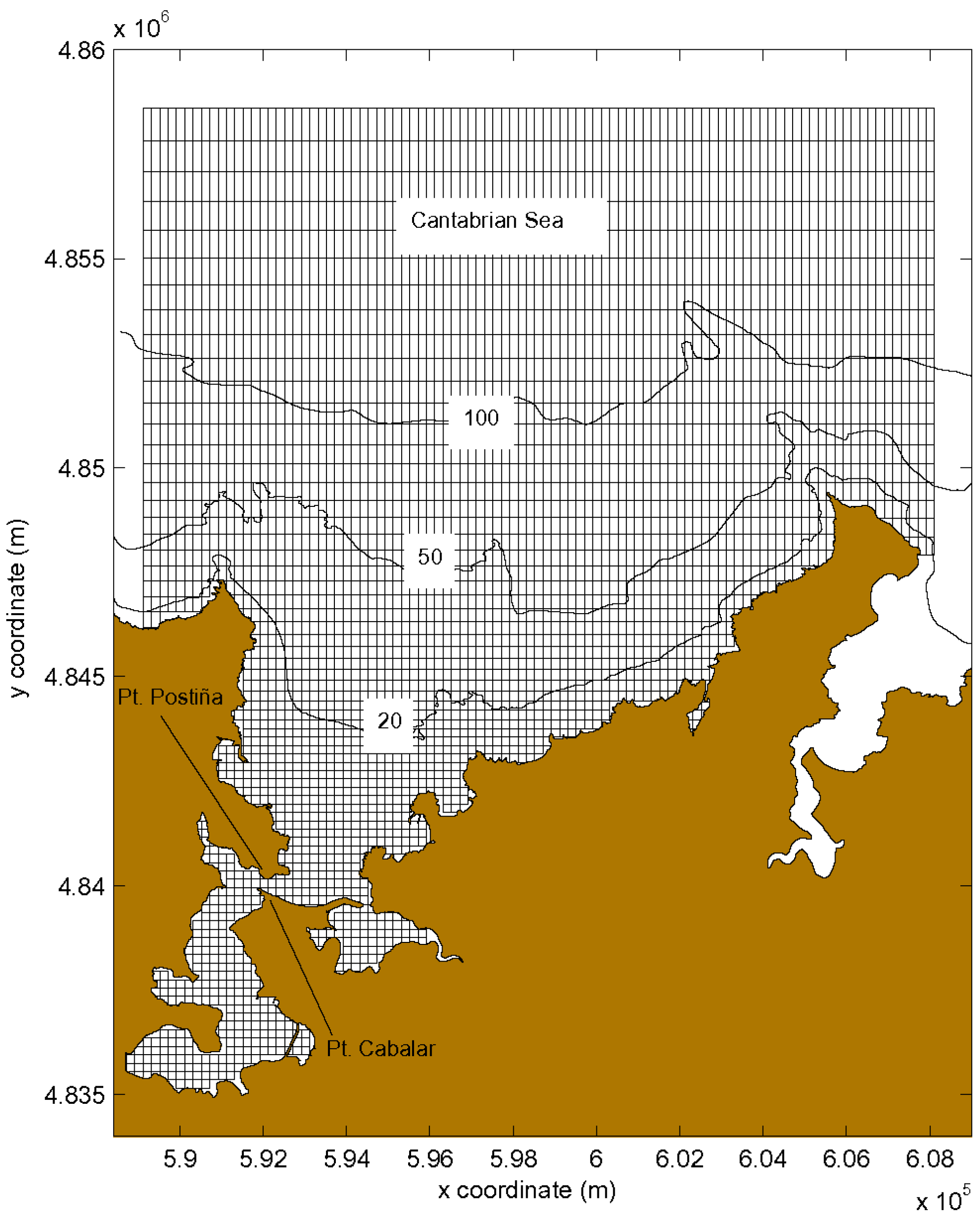
3.2. Numerical Model (II): Implementation
3.3. Tide-Driven Residual Circulation
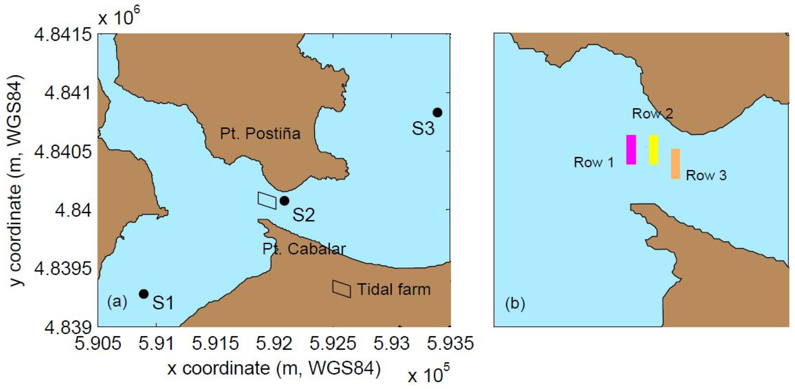
3.4. Case Studies
4. Results and Discussion
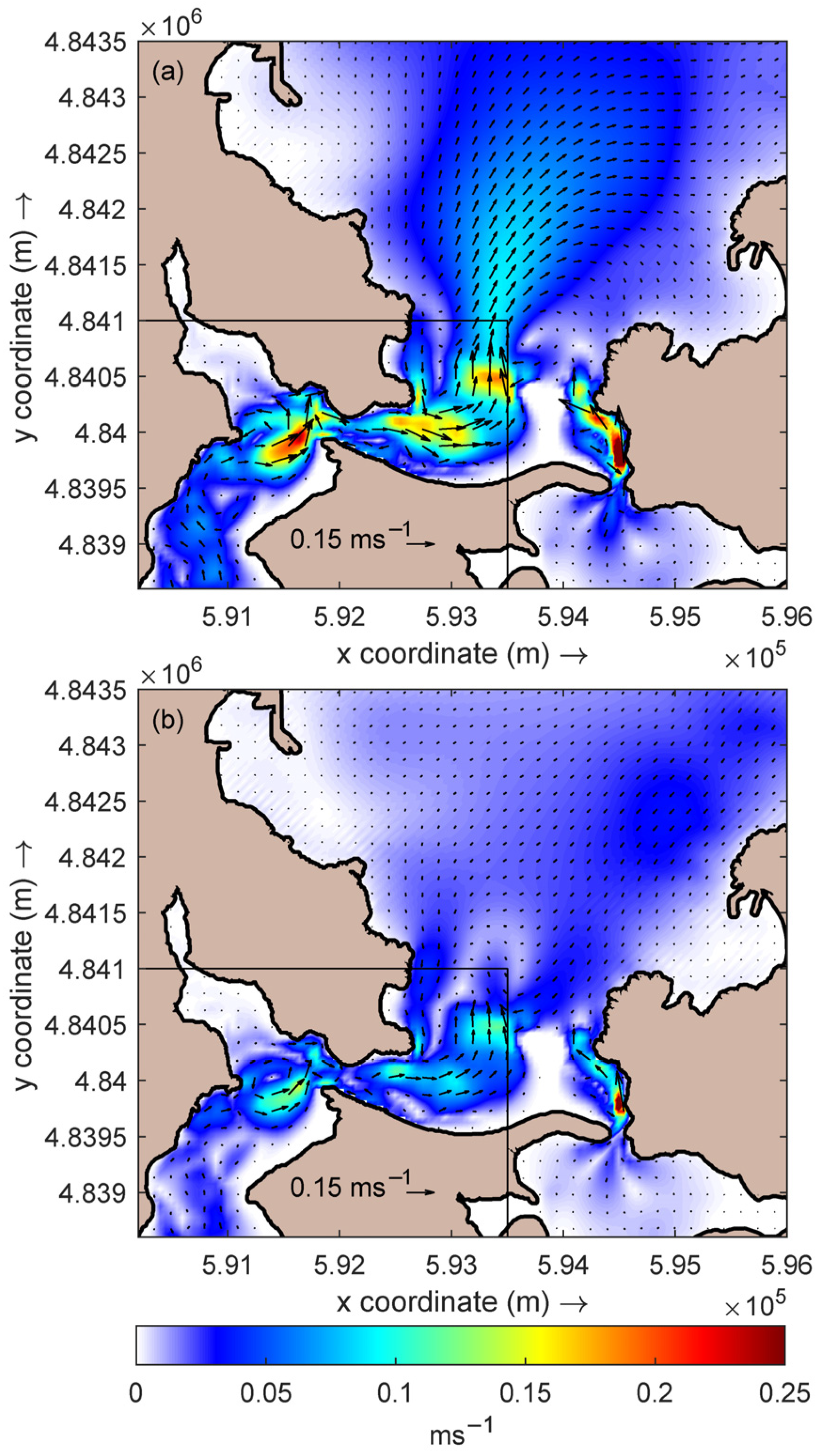
4.1. Unaltered Conditions
4.2. Altered Conditions
5. Conclusions
Author Contributions
Funding
Institutional Review Board Statement
Informed Consent Statement
Data Availability Statement
Acknowledgments
Conflicts of Interest
References
- Bekun, F.V.; Alola, A.A.; Sarkodie, S.A. Toward a sustainable environment: Nexus between CO2 emissions, resource rent, renewable and nonrenewable energy in 16-EU countries. Sci. Total Environ. 2019, 657, 1023–1029. [Google Scholar] [CrossRef]
- Pereira, F.; Neves, M.G.; López-Gutiérrez, J.-S.; Esteban, M.D.; Negro, V. Comparison of Existing Equations for the Design of Crown Walls: Application to the Case Study of Ericeira Breakwater (Portugal). J. Mar. Sci. Eng. 2021, 9, 285. [Google Scholar] [CrossRef]
- Fobissie, E.N. The role of environmental values and political ideology on public support for renewable energy policy in Ottawa, Canada. Energy Policy 2019, 134, 110918. [Google Scholar] [CrossRef]
- Herath, N.; Tyner, W.E. Intended and unintended consequences of US renewable energy policies. Renew. Sust. Energ. Rev. 2019, 115, 109385. [Google Scholar] [CrossRef]
- Nicolli, F.; Vona, F. Energy market liberalization and renewable energy policies in OECD countries. Energy Policy 2019, 128, 853–867. [Google Scholar] [CrossRef] [Green Version]
- Pischke, E.C.; Solomon, B.; Wellstead, A.; Acevedo, A.; Eastmond, A.; De Oliveira, F.; Coelho, S.; Lucon, O. From Kyoto to Paris: Measuring renewable energy policy regimes in Argentina, Brazil, Canada, Mexico and the United States. Energy Res. Soc. Sci. 2019, 50, 82–91. [Google Scholar] [CrossRef]
- Erdiwansyah; Mamat, R.; Sani, M.S.M.; Sudhakar, K. Renewable energy in Southeast Asia: Policies and recommendations. Sci. Total Environ. 2019, 670, 1095–1102. [Google Scholar] [CrossRef]
- European Commission Proposal for a Directive Amending Directive 98/70/EC Relating to the Quality of Petrol and Diesel Fuels and Amending Council Directive 93/12/EC and Amending Directive 2009/28/EC on the Promotion of the Use of Energy from Renewable Sources [COM(2012) 595]. 2012. Available online: https://eur-lex.europa.eu/legal-content/en/ALL/?uri=CELEX%3A32015L1513 (accessed on 16 October 2022).
- Portillo Juan, N.; Negro Valdecantos, V.; Esteban, M.D.; López Gutiérrez, J.S. Review of the Influence of Oceanographic and Geometric Parameters on Oscillating Water Columns. J. Mar. Sci. Eng. 2022, 10, 226. [Google Scholar] [CrossRef]
- Bahaj, A.S. Generating electricity from the oceans. Renew. Sust. Energy Rev. 2011, 15, 3399–3416. [Google Scholar] [CrossRef]
- Carballo, R.; Iglesias, G.; Castro, A. Numerical model evaluation of tidal stream energy resources in the Ría de Muros (NW Spain). Renew. Energy 2009, 34, 1517–1524. [Google Scholar] [CrossRef]
- Sánchez, M.; Carballo, R.; Ramos, V.; Iglesias, G. Energy production from tidal currents in an estuary: A comparative study of floating and bottom-fixed turbines. Energy 2014, 77, 802–811. [Google Scholar] [CrossRef]
- Esteban, M.D.; Espada, J.M.; Ortega, J.M.; López-Gutiérrez, J.-S.; Negro, V. What about Marine Renewable Energies in Spain? J. Mar. Sci. Eng. 2019, 7, 249. [Google Scholar] [CrossRef] [Green Version]
- European Commission. The Exploitation of Tidal Marine Currents; EUR16683EN; EC: Brussels, Belgium, 1996. [Google Scholar]
- Zarzuelo, C.; López-Ruiz, A.; Díez-Minguito, M.; Ortega-Sánchez, M. Tidal and subtidal hydrodynamics and energetics in a constricted estuary. Estuar. Coast. Shelf Sci. 2017, 185, 55–68. [Google Scholar] [CrossRef]
- Iglesias, G.; Sánchez, M.; Carballo, R.; Fernández, H. The TSE index—A new tool for selecting tidal stream sites in depth-limited regions. Renew. Energy 2012, 48, 350–357. [Google Scholar] [CrossRef]
- Fouz, D.M.; Carballo, R.; Ramos, V.; Iglesias, G. Hydrokinetic energy exploitation under combined river and tidal flow. Renew. Energy 2019, 143, 558–568. [Google Scholar] [CrossRef]
- Liu, Z.; Qu, H.; Shi, H. Numerical study on hydrodynamic performance of a fully passive flow-driven pitching hydrofoil. Ocean Eng. 2019, 177, 70–84. [Google Scholar] [CrossRef]
- Qian, P.; Feng, B.; Liu, H.; Tian, X.; Si, Y.; Zhang, D. Review on configuration and control methods of tidal current turbines. Renew. Sust. Energ. Rev. 2019, 108, 125–139. [Google Scholar] [CrossRef]
- Segura, E.; Morales, R.; Somolinos, J.A.; López, A. Techno-economic challenges of tidal energy conversion systems: Current status and trends. Renew. Sust. Energ. Rev. 2017, 77, 536–550. [Google Scholar] [CrossRef]
- Zhou, Z.; Benbouzid, M.; Charpentier, J.; Scuiller, F.; Tang, T. Developments in large marine current turbine technologies—A review. Renew. Sust. Energy Rev. 2017, 71, 852–858. [Google Scholar] [CrossRef]
- Ramos, V.; Carballo, R.; Álvarez, M.; Sánchez, M.; Iglesias, G. Assessment of the impacts of tidal stream energy through high-resolution numerical modeling. Energy 2013, 61, 541–554. [Google Scholar] [CrossRef]
- Ramos, V.; Carballo, R.; Sanchez, M.; Veigas, M.; Iglesias, G. Tidal stream energy impacts on estuarine circulation. Energy Conv. Manag. 2014, 80, 137–149. [Google Scholar] [CrossRef]
- Neill, S.P.; Jordan, J.R.; Couch, S.J. Impact of tidal energy converter (TEC) arrays on the dynamics of headland sand banks. Renew. Energy 2012, 37, 387–397. [Google Scholar] [CrossRef]
- Sánchez, M.; Carballo, R.; Ramos, V.; Iglesias, G. Tidal stream energy impact on the transient and residual flow in an estuary: A 3D analysis. Appl. Energy 2014, 116, 167–177. [Google Scholar] [CrossRef]
- Sanchez, M.; Carballo, R.; Ramos, V.; Iglesias, G. Floating vs. bottom-fixed turbines for tidal stream energy: A comparative impact assessment. Energy 2014, 72, 691–701. [Google Scholar] [CrossRef]
- Duarte, P.; Alvarez-Salgado, X.A.; Fernández-Reiriz, M.J.; Piedracoba, S.; Labarta, U. A modeling study on the hydrodynamics of a coastal embayment occupied by mussel farms (Ria de Ares-Betanzos, NW Iberian Peninsula). Estuar. Coast. Shelf Sci. 2014, 147, 42–55. [Google Scholar] [CrossRef] [Green Version]
- Díez, J. Las Costas; Alianza Editorial: Madrid, Spain, 1996. [Google Scholar]
- Alvarez, I.; Gomez-Gesteira, M.; de Castro, M.; Novoa, E.M. Ekman transport along the Galician Coast (NW, Spain) calculated from QuikSCAT winds. J. Mar. Syst. 2008, 72, 101–115. [Google Scholar] [CrossRef]
- Gómez-Gesteira, M.; de Castro, M.; Prego, R.; Pérez-Villar, V. An Unusual Two Layered Tidal Circulation Induced by Stratification and Wind in the Ría of Pontevedra (NW Spain). Estuar. Coast. Shelf Sci. 2001, 52, 555–563. [Google Scholar] [CrossRef]
- de Castro, M.; Gómez-Gesteira, M.; Alvarez, I.; Lorenzo, M.; Cabanas, J.M.; Prego, R.; Crespo, A.J.C. Characterization of fall-winter upwelling recurrence along the Galician western coast (NW Spain) from 2000 to 2005: Dependence on atmospheric forcing. J. Mar. Syst. 2008, 72, 145–158. [Google Scholar] [CrossRef]
- Blanton, J.O.; Atkinson, L.P.; Castillejo, F.; Lavin, A. Coastal upwelling off the Rias Bajas, Galicia, Northwest Spain I: Hydrographic Studies. Réun. Cons. Int. Explor. Mer. 1984, 183, 79–90. [Google Scholar]
- Villacieros-Robineau, N.; Herrera, J.L.; Castro, C.G.; Piedracoba, S.; Roson, G. Hydrodynamic characterization of the bottom boundary layer in a coastal upwelling system (Ría de Vigo, NW Spain). Cont. Shelf Res. 2013, 68, 67–79. [Google Scholar] [CrossRef] [Green Version]
- Alvarez-Salgado, X.A.; Roson, G.; Perez, F.F.; Pazos, Y. Hydrographic variability off the Rias Baixas (NW Spain) during the upwelling season. J. Geophys. Res. 1993, 98, 14447–14455. [Google Scholar] [CrossRef]
- Souto, C.; Gilcoto, M.; Fariña-Busto, L.; Pérez, F.F. Modeling the residual circulation of a coastal embayment affected by wind-driven upwelling: Circulation of the Ría de Vigo (NW Spain). J. Geophys. Res. 2003, 108, 4-1–4-18. [Google Scholar] [CrossRef] [Green Version]
- Herrera, J.L.; Rosón, G.; Varela, R.A.; Piedracoba, S. Variability of the western Galician upwelling system (NW Spain) during an intensively sampled annual cycle. An EOF analysis approach. J. Mar. Syst. 2008, 72, 200–217. [Google Scholar] [CrossRef]
- Prego, R.; Barciela, M.d.C.; Varela, M. Nutrient dynamics in the Galician coastal area (Northwestern Iberian Peninsula): Do the Rias Bajas receive more nutrient salts than the Rias Altas? Cont. Shelf Res. 1999, 19, 317–334. [Google Scholar] [CrossRef]
- Wooster, W.S.; Bakun, A.; McLain, D.R. Seasonal upwelling cycle along the eastern boundary of the North Atlantic. J. Mar. Res. 1976, 34, 131–141. [Google Scholar]
- Ríos, A.F.; Pérez, F.F.; Fraga, F. Water masses in the upper and middle North Atlantic Ocean east of the Azores. Deep Sea Res. Part A Oceanogr. Res. Pap. 1992, 39, 645–658. [Google Scholar] [CrossRef] [Green Version]
- Iglesias, G.; Carballo, R. Seasonality of the circulation in the Ría de Muros (NW Spain). J. Mar. Syst. 2009, 78, 94–108. [Google Scholar] [CrossRef]
- Alvarez, I.; Gomez-Gesteira, M.; de Castro, M.; Gomez-Gesteira, J.L.; Dias, J.M. Summer upwelling frequency along the western Cantabrian coast from 1967 to 2007. J. Mar. Syst. 2010, 79, 218–226. [Google Scholar] [CrossRef]
- Torres, R.; Barton, E.D.; Miller, P.; Fanjul, E. Spatial patterns of wind and sea surface temperature in the Galician upwelling region. J. Geophys. Res. 2003, 108, 3130. [Google Scholar] [CrossRef] [Green Version]
- Álvarez-Salgado, X.A.; Labarta, U.; Vinseiro, V.; Fernández-Reiriz, M.J. Environmental drivers of mussels flesh yield in a coastal upwelling system. Ecol. Indic. 2017, 79, 323–329. [Google Scholar] [CrossRef] [Green Version]
- Ospina-Alvarez, N.; Prego, R.; Álvarez, I.; de Castro, M.; Álvarez-Ossorio, M.T.; Pazos, Y.; Campos, M.J.; Bernárdez, P.; Garcia-Soto, C.; Gómez-Gesteira, M.; et al. Oceanographical patterns during a summer upwelling–downwelling event in the Northern Galician Rias: Comparison with the whole Ria system (NW of Iberian Peninsula). Cont. Shelf Res. 2010, 30, 1362–1372. [Google Scholar] [CrossRef] [Green Version]
- Sánchez, M.; Iglesias, G.; Carballo, R.; Fraguela, J.A. Power peaks against installed capacity in tidal stream energy. IET Renew. Power Gener. 2013, 7, 246–253. [Google Scholar] [CrossRef]
- Pugh, D.T. Tides, Surges, and Mean Sea-Level/a Handbook for Engineers and Scientists; John Wiley & Sons Inc.: Hoboken, NJ, USA, 1996; p. 486. [Google Scholar]
- Cerdeira-Arias, J.D.; Otero, J.; Barceló, E.; Río, G.d.; Freire, A.; García, M.; Nombela, M.Á.; Portilla, G.; Rodríguez, N.; Rosón, G.; et al. Hydrography of shellfish harvesting areas in the western Cantabrian coast (Rías Altas, NW Iberian Peninsula). Reg. Stud. Mar. Sci. 2018, 22, 125–135. [Google Scholar] [CrossRef]
- Iglesias, G.; Carballo, R. Effects of high winds on the circulation of the using a mixed open boundary condition: The Ría de Muros, Spain. Environ. Modell. Softw. 2010, 25, 455–466. [Google Scholar] [CrossRef]
- McClain, C.R.; Chao, S.Y.; Atkinson, L.P.; Blanton, J.O.; de Castillejo, F.F. Wind-driven upwelling in the vicinity of Cape Finisterre, Spain. J. Geophys. Res. 1986, 91, 8470–8486. [Google Scholar] [CrossRef] [Green Version]
- Alvarez, I.; Ospina-Alvarez, N.; Pazos, Y.; de Castro, M.; Bernardez, P.; Campos, M.J.; Gomez-Gesteira, J.L.; Alvarez-Ossorio, M.T.; Varela, M.; Gomez-Gesteira, M.; et al. A winter upwelling event in the Northern Galician Rias: Frequency and oceanographic implications. Estuar. Coast. Shelf Sci. 2009, 82, 573–582. [Google Scholar] [CrossRef]
- Deltares. User Manual Delft3D-FLOW; Deltares: Delft, The Netherlands, 2010. [Google Scholar]
- Philips, N.A. A co-ordinate system having some special advantages for numerical forecasting. J. Meteorol. 1957, 14, 184–185. [Google Scholar] [CrossRef]
- Carballo, R.; Iglesias, G.; Castro, A. Residual circulation in the Ría de Muros (NW Spain): A 3D numerical model study. J. Mar. Syst. 2009, 75, 130. [Google Scholar] [CrossRef]
- Iglesias, G.; Carballo, R. Can the seasonality of a small river affect a large tide-dominated estuary? The case of the Ria de Viveiro, Spain. J. Coast. Res. 2011, 27, 1170–1182. [Google Scholar] [CrossRef]
- Torres López, S.; Varela, R.A.; Delhez, E. Residual circulation and thermohaline distribution of the Ría de Vigo: A 3-D hydrodynamic model. Sci. Mar. 2001, 65, 277–289. [Google Scholar] [CrossRef] [Green Version]
- Dias, J.M.; Lopes, J.F. Implementation and assessment of hydrodynamic, salt and heat transport models: The case of Ria de Aveiro Lagoon (Portugal). Environ. Modell. Softw. 2006, 21, 1–15. [Google Scholar] [CrossRef]
- Cheng, R.T.; Casulli, V.; Gartner, J.W. Tidal, Residual, Intertidal Mudflat (TRIM) Model and its Applications to San Francisco Bay, California. Estuar. Coast. Shelf Sci. 1993, 36, 235–280. [Google Scholar] [CrossRef]
- Cheng, R.T.; Gartner, J.W. Harmonic analysis of tides and tidal currents in South San Francisco Bay, California. Estuar. Coast. Shelf Sci. 1985, 21, 57–74. [Google Scholar] [CrossRef]
- Smith, S.D. Wind stress and heat flux over the ocean in gale force winds. J. Phys. Oceanogr. 1980, 10, 709–726. [Google Scholar] [CrossRef]
- Yelland, M.J.; Moat, B.I.; Taylor, P.K.; Pascal, R.W.; Hutchings, J.; Cornell, V.C. Wind stress measurements from the open ocean corrected for airflow distortion by the ship. J. Phys. Oceanogr. 1998, 28, 1511–1526. [Google Scholar] [CrossRef]
- Stelling, G.; Leendertse, J. Approximation of convective processes by cyclic ADI methods. In Proceedings of the 2nd ASCE Conference on Estuarine and Coastal Modelling, Tampa, FL, USA, 13–15 November 1992. [Google Scholar]
- Chung, T.J. Computational Fluid Dynamics; Cambridge University Press: Cambridge, UK, 2002; p. 1012. [Google Scholar]
- Rodi, W. Examples of calculation methods for flow and mixing in stratified fluids. J. Geophys. Res. 1987, 92, 5305–5328. [Google Scholar] [CrossRef]
- Defne, Z.; Haas, K.A.; Fritz, H.M. Numerical modeling of tidal currents and the effects of power extraction on estuarine hydrodynamics along the Georgia coast, USA. Renew. Energy 2011, 36, 3461–3471. [Google Scholar] [CrossRef]
- Shapiro, G.I. Effect of tidal stream power generation on the region-wide circulation in a shallow area. Ocean Sci. 2011, 7, 165–174. [Google Scholar] [CrossRef] [Green Version]
- Bahaj, A.S.; Molland, A.F.; Chaplin, J.R.; Batten, W.M.J. Power and thrust measurements of marine current turbines under various hydrodynamic flow conditions in a cavitation tunnel and a towing tank. Renew. Energy 2007, 32, 407–426. [Google Scholar] [CrossRef]
- Álvarez, M.; Ramos, V.; Carballo, R.; López, I.; Fouz, D.M.; Iglesias, G. Application of Marine Spatial Planning tools for tidal stream farm micro-siting. Ocean Coast. Manag. 2022, 220, 106063. [Google Scholar] [CrossRef]
- Myers, L.E.; Bahaj, A.S. An experimental investigation simulating flow effects in first generation marine current energy converter arrays. Renew. Energy 2012, 37, 28–36. [Google Scholar] [CrossRef] [Green Version]
- Umgiesser, G. Modelling the Venice Lagoon. Int. J. Salt Lake Res. 1997, 6, 177–199. [Google Scholar] [CrossRef]
- Salas-de-León, D.A.; Carbajal-Pérez, N.; Monreal-Gómez, M.A.; Barrientos-MacGretor, G. Residual circulation and tidal stress in the Gulf of California. J. Geophys. Res. 2003, 108, 3317. [Google Scholar] [CrossRef]


| Constituent | Amplitude (cm) | Phase (°) |
|---|---|---|
| M2 | 122.79 | 90.15 |
| S2 | 42.91 | 121.08 |
| N2 | 25.98 | 70.39 |
| K2 | 12.03 | 118.76 |
| K1 | 7.35 | 73.49 |
| O1 | 6.22 | 324.62 |
| P1 | 2.22 | 65.15 |
| Q1 | 2.11 | 271.31 |
| M4 | 1.45 | 334.80 |
| Scenario | River Discharge Conditions | Oceanic Conditions | |||
|---|---|---|---|---|---|
| River Flow (m3 s−1) | Salinity (ppt) | Temperature (°C) | Salinity (ppt) | Temperature (°C) | |
| Spring–summer | 3.07 | 0.051 | 15.60 | 35.68 | 15.51 |
| Autumn–winter | 8.48 | 0.051 | 11.10 | 35.48 | 13.17 |
| D (m) | Vci (ms−1) | Vr (ms−1) | Vco (ms−1) | A (m2) | Pr (kW) | CpNO | CpSC |
|---|---|---|---|---|---|---|---|
| 5 | 0.7 | 2.2 | 3.1 | 19.6 | 40 | 0.35 | 0.2 |
| Case Study | Tidal Plant | Wind | Fluvial and Oceanic Conditions (Table 2) |
|---|---|---|---|
| CS1 | No plant | No wind | Spring–summer |
| CS2 | No plant | No wind | Autumn–winter |
| CS3 | No plant | SW mean summer wind (3.32 ms−1) | Spring–summer |
| CS4 | No plant | SW mean winter wind (6.03 ms−1) | Autumn–winter |
| CS5 | Floating plant | No wind | Autumn–winter |
| CS6 | Bottom plant | No wind | Autumn–winter |
| CS7 | Floating plant | SW mean winter wind (6.03 ms−1) | Autumn–winter |
| CS8 | Bottom plant | SW mean winter wind (6.03 ms−1) | Autumn–winter |
Publisher’s Note: MDPI stays neutral with regard to jurisdictional claims in published maps and institutional affiliations. |
© 2022 by the authors. Licensee MDPI, Basel, Switzerland. This article is an open access article distributed under the terms and conditions of the Creative Commons Attribution (CC BY) license (https://creativecommons.org/licenses/by/4.0/).
Share and Cite
Sánchez, M.; Fouz, D.M.; López, I.; Carballo, R.; Iglesias, G. Effects of Tidal Stream Energy Exploitation on Estuarine Circulation and Its Seasonal Variability. J. Mar. Sci. Eng. 2022, 10, 1545. https://doi.org/10.3390/jmse10101545
Sánchez M, Fouz DM, López I, Carballo R, Iglesias G. Effects of Tidal Stream Energy Exploitation on Estuarine Circulation and Its Seasonal Variability. Journal of Marine Science and Engineering. 2022; 10(10):1545. https://doi.org/10.3390/jmse10101545
Chicago/Turabian StyleSánchez, Marcos, David Mateo Fouz, Iván López, Rodrigo Carballo, and Gregorio Iglesias. 2022. "Effects of Tidal Stream Energy Exploitation on Estuarine Circulation and Its Seasonal Variability" Journal of Marine Science and Engineering 10, no. 10: 1545. https://doi.org/10.3390/jmse10101545