Exploring the Potential Use of Sentinel-1 and 2 Satellite Imagery for Monitoring Winter Wheat Growth under Agricultural Drought Conditions in North-Western Poland

Abstract

This paper presents analyses of the potential use of Sentinel-1 (S-1) and Sentinel-2 (S-2) imagery to generate models of winter wheat growth under agricultural drought vs. normal conditions identified based on potential yield losses calculated in the Agricultural Drought Monitoring System (ADMS). The analyses carried out showed the sensitivity of satellite images to agricultural drought conditions determined in ADMS. The study was conducted in a large region, the West Pomeranian Voivodeship (NUTS PL42), and the analysis covered about 22,935 polygons with winter wheat production that constituted a total area of about 108,000 ha in the period from the 1st of April to the 1st of July 2021. For S-1 data, VH and VV backscatter and the VH/VV ratio were calculated, and for S-2 data, NDVI and NDWI indices were calculated, which were used to build models of winter wheat growth under water stress and in normal conditions. The obtained results presented in this work include: (i) Development of a test version of a model describing the winter wheat crop’s growth, with a preliminary assessment showing the potential for recognizing water shortage effects; and (ii) identification of promising indicators of water scarcity for crops, calculated based on S-1 and S-2 images, that could be recommended for application in remote sensing (RS) of drought effects as complementary multispectral and radar observations. The results obtained in this work also gave many clues regarding the direction and method of including satellite remote sensing in national monitoring programmes, which involves operations on many types of big data sets.

1. Introduction

Satellite imagery used for agricultural applications allows the phenomena under study to be observed either temporally or spatially, depending on the image resolution, from global to field scale, i.e., drought monitoring [1], plant freezing [2], crop overwintering assessment [3], yield forecasting [4], crop identification [5], plant disease and pest detection [6,7], precision agriculture [8,9]. However, so far, these studies have been expensive. The imagery delivered by the European Space Agency, in the Copernicus Programme, has changed this situation by providing free remote sensing data. In particular, the Sentinel-1 (S-1) and Sentinel-2 (S-2) mission’s data make it possible to observe the Earth’s surface with a spatial resolution starting at about 10 m and a frequency in Europe of about 5–6 days. Several studies are being conducted to explore the potential utilization of Sentinel-1 and Sentinel-2 imagery, separately and as a synergy, to provide support for the development and management of agriculture [10,11,12,13]. The synergy of S-1 and S-2 imagery is being investigated for the reason that optical data from S-2, unlike radar data from S-1, are often disturbed by cloudiness and do not allow ongoing observations during crucial growth stages of crops. However, radar data require different interpretation than optical data, which are influenced by various factors such as moisture and the physical structure of the plant [14], so many ongoing studies are exploring the possibility of interpreting the results obtained from S-1 using S-2 data. Therefore, S-1 may be useful for, e.g., monitoring phenological phases of plants [15], where the authors of the study, using neural networks, obtained an average accuracy of 93.5% for the separation of rice phenological phases, and the average error between the calculated and actual phenological date was 3.08 days; crop classification based on temporal signatures with a supervised approach [16], where the author achieved an overall accuracy higher than 70%, or crop classification using the Random Forest method [17], where the 48 crop groups could be classified with an overall accuracy of 93.4%; monitoring crop height [18], where the authors showed a strong relationship between maize height and SAR parameters, with the coefficient of determination for VV + VH (R² = 0.82), VV (R² = 0.81), and VH (R² = 0.80); selection of the optimal machinery type for sugarcane field cultivation [19], where authors developed a mathematical model and received an accuracy of 83.6% and 81.2% for the training and testing models, respectively; monitoring plant development [20,21,22], where authors showed a high sensitivity of the indicators provided by S-1 to the detection of phenological growth stages for different crops; or testing sensitivity to agricultural drought [23,24], where authors found a correlation between backscatter as well as interferometric data and crop water stress. On the other hand, S-2 is more suitable for yield prediction [25,26] since authors reported a strong correlation between the obtained yield and vegetation indices with R² values ranging from 0.6 to 0.9; precision nitrogen fertilization [27], where authors showed that NDVI data can be used for field-scale optimal nitrogen management models; or detailing the soil-agricultural map [28]. The synergy of S-1 and S-2 could, therefore, be applied to, e.g., monitoring phenological phases of plants [29], where authors found that the highest identification of phenological phases was obtained for a combination of optical and SAR data in comparison to using these data separately; agricultural drought monitoring [30], where authors indicated that the synergy of these data can be a useful indicator of crop condition, especially for corn and sunflower, with prediction rates of 86% and 71%, respectively; monitoring crop parameters [31,32] such as plant’s growth and height; crop identification [33,34,35], where authors obtained maximum crop classification accuracy of 85%, 75%, and 86%, respectively; or determination of soil properties [36], where applied models showed a prediction accuracy of 94%, 89%, and 96% for pH, SOM and clay content, respectively.

Since the synthetic aperture radar (SAR) response depends on geometric and dielectric properties, it is expected that water scarcity caused by drought should be visible in the SAR response. The radar signal reflected by plant tissues under normal conditions with proper vigor should be different from the plant’s response affected by water stress. Plant status evaluated with the use of radar data (images) should be correlated with the results of methods based on the analysis of multispectral images using vegetation indices derived from S-2 images. Combining these two methods enables monitoring of plant status under different weather conditions, e.g., periods of high cloudiness, and the relationship between vegetation indices calculated from multispectral images and ground observations is very well documented in the literature and can support the interpretation of indices extracted from radar images. Demonstrating these relationships and the possibility of their implementation in the drought monitoring system is the main purpose of this work.

The novelty of this work is: (i) demonstrating the potential of Sentinel-1 and Sentinel-2 imagery in detecting agricultural drought at a regional scale; (ii) generating a model of winter wheat growth and development under normal and agricultural drought conditions for the region; and (iii) providing regional analyses of study crops for a large research sample.

2. Materials and Methods

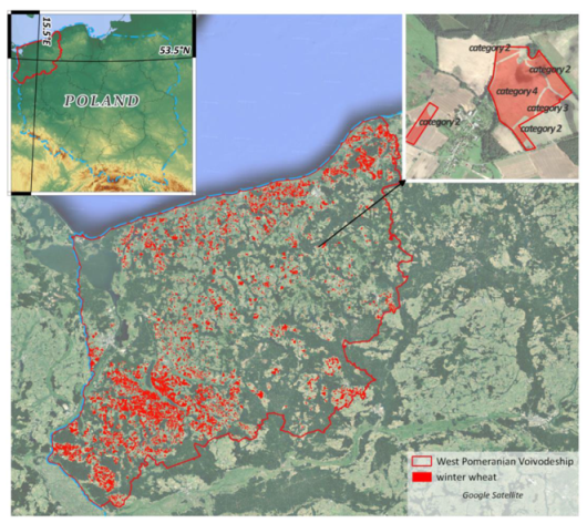
2.1. Study Area Location

The research area consisted of 21,850 fields of winter wheat, each larger than 0.5 ha, located in the West Pomeranian Voivodeship (NUTS PL42) [37], in the north-western part of Poland. This region of the country is characterized by the largest average farm size of about 32 ha [38]. In the case of this study, the average field size was 7 ha, and the total analyzed area was about 145,750 ha (Figure 1).

Soil and climatic conditions in the West Pomeranian Voivodeship contribute to agricultural development; in this region, soils of medium value predominate—classes IVa and IVb, which cover around 50% of all arable land [39]. The most favorable soil conditions are found in the south-western part of the province, and the poorest soils are in the south-eastern part of the region. The climate of the West Pomeranian region results from the interaction between maritime and terrestrial climates as well as the influence of local factors. The northern and western parts of the voivodeship are characterized by a maritime climate. However, along with the increasing distance from the Baltic Sea towards the east, the features of a continental climate are perceptible. On average, the annual air temperature ranges from 7.0 °C to 8.5 °C, and the annual precipitation ranges from 490 to 770 mm in this region.

Winter wheat (Triticum aestivum L.) fields were chosen for the study because this crop covers the largest part of the agricultural land in this region of the country, and the research period ran from April to July 2021. The meteorological conditions during the autumn of 2020 were optimal, and the crop was characterized by good overwintering, which created conditions for good growth and development of the winter wheat in the spring of 2021. Daily air temperature variations allowed plants to become well tempered. In March, winter plants re-started growth at the usual time for this region of the country [40]. However, the Agricultural Drought Monitoring System (ADMS) conducted by the Institute of Soil Science and Plant Cultivation (IUNG-PIB) recorded the most intense drought for winter cereals in a few sub-regions of the West Pomeranian Voivodeship. This created very favorable conditions for testing the effect of drought on winter wheat development as registered by S-1 and S-2 data at the regional scale.

2.2. Materials

For this research, the following databases were used:

• Agricultural Drought Monitoring System (ADMS): a soil drought vulnerability category map describing the soil variability, climatic water balance (CWB) maps, and estimated yield losses [41,42]
• Agency for Restructuring and Modernization of Agriculture (ARMA): field boundaries used for direct payments [43]
• European Space Agency, Copernicus Programme: Sentinel-2 and Sentinel-1 satellite images [44].

2.2.1. Agricultural Drought Monitoring System Data

The ADMS uses a combination of databases and computer applications integrating meteorological data and soil-agricultural maps to present the spatial heterogeneity of water retention in different soil drought vulnerability categories. In the ADMS, the occurrence of agricultural drought is showcased in 14 reports between the 21st of March and the 30th of September when the CWB values calculated for each reporting period are lower than defined in the “Act on subsidies to insurance of agricultural crops and farm animals in Poland” [45] according to specific crop species or groups (also defined in the Act) and soil categories. For each reporting period using CWB values, the yield loss caused by agricultural drought is calculated in respect of the monitored crops, and the maximum loss for the entire season is the highest value found in a single report. Reports are published every 10 days, and the presented results cover 60 days from the date of their publication. Drought risk analysis is reported on winter cereals in nine reports from the 21st of March to the 10th of August [46].

Soil Drought Vulnerability Category Map

ADMS, in order to determine areas affected by agricultural drought, takes into account not only CWB values but also soil texture derived from soil-agricultural maps, which determines the available water capacity of the soil. This allowed us to distinguish four soil drought vulnerability categories (

Table 1. Description of soil drought vulnerability categories.

Name	Description	Available Water Capacity (AWC)
Category I	Highly sensitive to drought	<127.5 mm
Category II	Sensitive to drought	127.5–169.9 mm
Category III	Moderately sensitive to drought	170.0–202.5 mm
Category IV	Slightly sensitive to drought	>202.5 mm

Source: [47,48].

).

Climatic Water Balance (CWB) Maps and Yield Loss Estimation

To determine the areas with agricultural drought hazards, the ADMS IT system generates CWB maps, calculated from the difference between the amount of precipitation and potential evapotranspiration. Geospatial precipitation raster data are collected from ground-based meteorological radars of the POLRAD network, which is managed by the Institute of Meteorology and Water Management-National Research Institute (IMWM-PIB), while the potential evapotranspiration is calculated by the Penman method using data obtained from a network of meteorological stations distributed throughout Poland. Based on the values from the CWB maps, and taking into account the soil drought vulnerability category, potential yield losses for specific agricultural crops were determined.

More information on the functioning of the ADMS and the yield loss estimation methods can be found in Doroszewski and Górski [49], Doroszewski et al. [50], Szewczak et al. [51], Bartosiewicz and Jadczyszyn [52], and Jędrejek et al. [12].

2.2.2. Agency for Restructuring and Modernization of Agriculture Data

Field boundaries in SHP format were obtained from the ARMA database, which collects this data to determine the acreage of crops grown on farms needed for the distribution of direct payments to farmers. All polygons were pre-processed, and objects with attributes of winter wheat were selected for further analysis.

2.2.3. European Space Agency Data

The Sentinel series of space missions under the Copernicus Programme have been carried out by the European Space Agency, which provides member countries with free access to all data acquired under this project.

Sentinel-1

The Sentinel-1 (S-1) mission consisted of two satellites, 1A and 1B (deactivated on 23 December 2021), equipped with SAR radar sensors operating in C-band. The constellation of these satellites and the technical parameters of the sensors allowed the entire globe to be imaged within 6 days with a spatial resolution of 10 m [53].

Sentinel-2

The Sentinel-2 (S-2) mission consists of two satellites, 2A and 2B, equipped with a 13-channel multispectral scanner in the visible radiation range, capturing imagery with a spatial resolution of 10, 20, and 60 m (depending on the band). The revisit time for the satellite pair is 5 days [54].

Both satellites, S-1 and S-2, are shifted 180 degrees relative to each other and operate in a heliosynchronous orbit.

2.3. Methods and Scenario of the Analysis

The analyses were conducted in five successive stages: (1) preparation of polygon winter wheat fields for analysis; (2) calculation of potential yield loss based on CWB; (3) maps of indices from S-2 and S-1 data; (4) time series modeling of winter wheat growth variability under different weather conditions; and (5) methods of comparing the index variability function over time.

• Step 1: Preparation of Polygons Winter Wheat Fields for Analysis

Winter wheat field boundaries were intersected with the soil drought vulnerability category map. Then, a 10 m negative buffer was made for the newly created polygons in order to reduce the influence caused by the boundaries between the soil drought susceptibility categories on the calculated satellite indicator values (Figure 1). Each polygon was assigned a category of soil drought vulnerability. New polygons created under this intersection were the basis for further analysis, which covered only those exceeding or equal to 0.5 hectares. Finally, 22,935 polygons were analyzed. The total area covered by this analysis was 107,676 ha.

• Step 2: Calculation of Potential Yield Loss Based on CWB

For the prepared polygons from step one, based on the climatic water balance maps generated in ADMS, potential yield losses of winter wheat caused by water scarcity were calculated. These losses were computed using the values from the CWB maps, according to the original formulas developed at IUNG-PIB, with respect to soil categories for winter cereals in nine reporting periods (Figure 2). Thus, yield losses in nine periods were calculated for each winter wheat polygon from step 1. By selecting the maximum values of losses obtained from partial reports, the maximum winter wheat yield losses that occurred in 2021 were calculated. As an outcome in step 2, each polygon received attributes of potential yield losses over the nine reporting periods as well as maximum reached yield losses.

• Step 3: Maps of Indices from S-2 and S-1 Data

Sentinel-1A and Sentinel-1B images produced from the 1st of April to the 1st of July 2021 were downloaded from the ESA servers (ESA 2023). The studied fields were located in six passes of the Sentinel-1 satellite (ascending relative orbits A146, A73, and A175; descending relative orbits D95, D22, and D124).

The pre-processing of Sentinel-1 images to sigma nought (σ₀) was realized using the ESA SNAP toolbox [55]. The data were downloaded as Level-1 Ground Range Detected (GRD) products. GRD border noise was removed. The data were calibrated to convert the digital numbers received from the satellite into backscatter coefficients. The thermal noise in the data was removed to enhance the overall quality of the image. For the terrain correction, the COPERNICUS GLO-30 Digital Elevation Model was applied. This step accounts for the influence of topography on the radar signal by applying a correction based on the elevation information provided by the GLO-30 model. The data were radiometrically calibrated to convert the backscatter coefficients to sigma nought values. Sigma nought represents the radar backscatter coefficient normalized to the radar’s incident angle. All the obtained values were converted to a logarithmic scale with the unit decibel (dB). Speckle reduction was not conducted to ensure unbiased data values. As a result of this processing, backscatter images were obtained for the two polarizations: vertical-vertical (VV) and vertical-horizontal (VH). The median backscatter of VH and VV was calculated for each surveyed polygon from step 2, and based on these values, the VH/VV ratio was also obtained.

Sentinel-2A and Sentinel-2B images were downloaded from the ESA servers [44] with Level 2A processing, which stores bottom of atmosphere (BOA) reflectance information after atmospheric correction. The studied fields were located in eight Sentinel-2 granules (33UXU, 33UWU, 33UVU, 33UXV, 33UWV, 33UVV, 33UXA, and 33UWA). For all downloaded images, the cloud and shadow probability mask (CLDPRB) provided by ESA were used. For further analysis, only image fragments with no cloud cover within the investigated polygons during the whole investigation period were selected to keep the tested area of the fields constant.

From the numerous vegetation indices (VIs) that can be calculated from S-2 image channels [56], two were selected for the purpose of the study: the Normalized Difference Vegetation Index (NDVI)—detecting crop health and stage development—and the Normalized Difference Water Index (NDWI)—canopy water content sensitive.

NDVI is the most commonly used and documented VIs in the literature, used in agriculture to monitor vegetation dynamics [57,58].

$$\mathrm{N}\mathrm{D}\mathrm{V}\mathrm{I}=\frac{\mathrm{B}8-\mathrm{B}4}{\mathrm{B}8+\mathrm{B}4}$$

(1)

where B8 = NIR S-2 band (0.785–0.900 μm); B4 = RED S-2 band (0.650–0.680 μm);

NDWI was introduced by Gao in 1996 [59]. This VIs is a useful indicator for the detection of plant liquid water content and has less sensitivity to atmospheric dispersion effects than NDVI.

$$\mathrm{N}\mathrm{D}\mathrm{W}\mathrm{I}=\frac{\mathrm{B}8-\mathrm{B}11}{\mathrm{B}8+\mathrm{B}11}$$

(2)

where B8 = NIR S-2 band (0.785–0.900 μm); B11 = SWIR1 S-2 band (1.565–1.655 μm);

As a result of the analyses performed in this step, maps of NDVI and NDWI indices from S-2 and VV, VH, and VH/VV from S-1 were obtained.

• Step 4: Time Series Modelling of Winter Wheat Growth Variability under Different Weather Conditions

Based on the results from Step 3, for each study polygon (Step 2), a median value of the analyzed S-1 and S-2 indices was calculated with the assigned date of satellite observation. The study dataset was categorized into two subsets, according to the yield losses estimated by the ADMS (calculated in step 2). The first subset contained yield losses below 15% (considered no significant agricultural drought or lack of drought), and the second subset comprised losses above 35% (observable high impact of agricultural drought on winter wheat plants). Yield losses between 15 and 35% were excluded from the analyses, being considered an intermediate condition between those with visible and non-visible agricultural drought impact on the growth and development of winter wheat. To visualize winter wheat growth fluctuations, a moving window method in a 10-day step was used to smooth and reduce the noise of daily outlier data variations. For smoothing the time series of the studied indices, the median was taken from the interval of the time series value covering observations around the current value, including itself. In total, 775,508 S-1 observations and 186,507 S-2 observations were used to create a winter wheat growth variability function under both drought and no drought conditions. Due to the lack of normal distribution in the sets of the S-1 and S-2 index values for individual fields, non-parametric dispersion measures (median and MAD) were used (Formula (1)). MAD is the median of the absolute deviations from the median and is robust to data outliers [60].

$$MAD=b M_i\left(\left|x_i-M_j\left(x_j\right)\right|\right)$$

(3)

where x_i—n original observations; M_i—median of the series; b—constant;

Trimming the data by MAD was done to eliminate data outliers caused by other factors, e.g., damage caused by pests and diseases, biomass, and greenness change caused by weed infestation or improper crop cultivation.

• Step 5: Methods of Comparing the Index Variability Function over Time

The dynamics of index volatility over time were analyzed using two methods: (i) visual analysis, where the course of average index values and deviations in the entire observation period was initially presented using functions and diagrams; and (ii) descriptive analysis, where the differences between the average values of the indices observed in 10-day intervals in drought-prone and drought-free regions were compared.

To visualize the course of index variability in a study period, a script was written in the R environment [61]. This algorithm generates diagrams of the development and growth of winter wheat for a 10-day moving window. The created diagrams were composed of error bars meaning +/−1 MAD (black vertical bars) from the median of the 10-day dataset (red dots) and an estimated smoothed winter wheat growth function (blue line).

Descriptive analysis with tabular descriptions is one of the qualitative methods used in research that aims to assess some characteristics of a specific population or situation. Usually, this type of research opens the way to deeper and more complex research on a given phenomenon, presenting, for example, as in this study, the periods during which we should expect to find answers to the presented research problem. For this type of analysis, various statistical software can be used, of which Excel was chosen for this study.

3. Results

The calculated potential yield losses according to IUNG (step 2) for the study area ranged from 0 to 55%.

Figure 3, Figure 4, Figure 5, Figure 6 and Figure 7 present the variability and development of indices derived from S-1 and S-2 images over the season for normal and drought conditions and a comparison of the two functions. On the left (A), the course of variability of index values in standard conditions is presented; on the right (B), in conditions of water shortage causing yield losses greater than 35%. In addition, the median values (red dots) and the error bars show the range of +/−1MAD. In all C figures, a comparison of the variability and development of the indices over time for standard and water-limited conditions is presented.

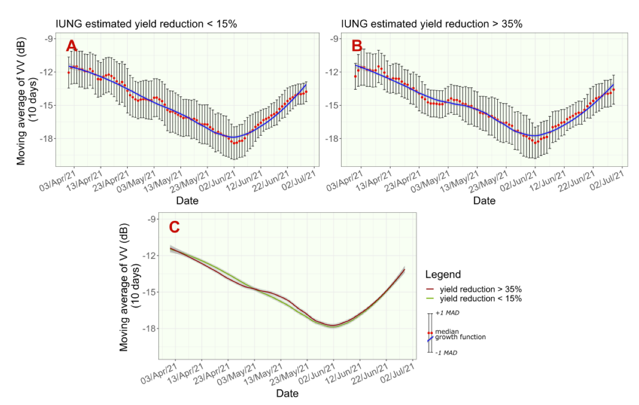
3.1. Variability and Development of Vegetation Indices Derived from Sentinel-2 Images

For Sentinel-2, graphs of NDVI (Figure 3) and NDWI (Figure 4) development were created. Higher differences between the two datasets of fields (normal and agricultural drought conditions) were observed for NDWI (Figure 4C) and slightly smaller for NDVI (Figure 3C). This may be due to the fact that the NDWI index is a so-called drought index, which measures canopy water content and is a very good indicator of the plant’s water stress, while the NDVI index values are more correlated with the quantity of biomass and chlorophyll content. It is also confirmed by other studies that the NDWI index is more sensitive to agricultural drought detection than the NDVI, which was proved, e.g., in a semi-arid region of Zacatecas, Mexico [62].

In the case of NDWI, a better separation is also observed between the functions describing the average index values for the separated ranges of yield losses (Figure 4A,B). These differences are the most visible for the period from 13 April to 12 May and from 2 June onwards, i.e., from the period of plant maturation and loss of greenness.

Figure 3. NDVI variability and development over the season for (A) normal conditions, (B) drought conditions, and (C) a comparison of the two NDVI functions. Source: own study.

Figure 3. NDVI variability and development over the season for (A) normal conditions, (B) drought conditions, and (C) a comparison of the two NDVI functions. Source: own study.

Figure 4. NDWI variability and development over the season for (A) normal conditions, (B) drought conditions, and (C) a comparison of the two NDWI functions. Source: own study.

Figure 4. NDWI variability and development over the season for (A) normal conditions, (B) drought conditions, and (C) a comparison of the two NDWI functions. Source: own study.

3.2. Variability and Development of Indices Derived from of Sentinel-1 Images

Spatially averaged at the field level, values of VV, VH, and VH/VV derived from S-1 images showed that the growth and development pattern of winter wheat (expressed by these indices) grown under no-drought conditions (Figure 5A, Figure 6A and Figure 7A) and drought conditions (Figure 5B, Figure 6B and Figure 7B) varied the most significantly for backscatter VH (Figure 6C) and for cross ratio VH/VV (Figure 7C). When using the VV index, the differences in winter wheat development were almost invisible (Figure 6C).

Higher values of the VH index were observed in early spring for winter wheat not affected by drought (Figure 5A) in comparison with the VH values for winter wheat affected by drought (Figure 5B) during the period of rapid plant growth. However, an opposite situation was faced after 13 May (Figure 5C), when the lines of VH development intersected and higher values of VH were observed for wheat grown under drought conditions.

The differences between the VV backscatter functions developed for wheat grown under normal and agricultural drought conditions were much less visible. In addition, an intersection of the functions was observed earlier, around 3 May (Figure 6C).

Variability and development of the VH/VV ratio over the season were similar to the results obtained for the VH index, where during the period of rapid winter wheat growth (till mid-May), higher VH/VV ratio values were found for winter wheat grown under normal conditions (Figure 7A) compared to VH/VV values observed for wheat from fields under drought conditions (Figure 7B). Around 18 May, the lines showing VH/VV variability for winter wheat fields under different weather conditions had intersected (Figure 7C), and afterwards the course of the VH/VV functions had reversed. Higher VH/VV values were noted under conditions with a water deficit (Figure 7B) compared to conditions without water scarcity (Figure 7A).

Figure 5. VH variability and development over the season for (A) normal conditions, (B) drought conditions, and (C) a comparison of the two VH functions. Source: own study.

Figure 5. VH variability and development over the season for (A) normal conditions, (B) drought conditions, and (C) a comparison of the two VH functions. Source: own study.

Figure 6. VV variability and development over the season for (A) normal conditions, (B) drought conditions, and (C) a comparison of the two VV functions. Source: own study.

Figure 6. VV variability and development over the season for (A) normal conditions, (B) drought conditions, and (C) a comparison of the two VV functions. Source: own study.

Figure 7. Ratio of VH/VV variability and development over the season for (A) normal conditions, (B) drought conditions, and (C) a comparison of the two VH/VV functions. Source: own study.

Figure 7. Ratio of VH/VV variability and development over the season for (A) normal conditions, (B) drought conditions, and (C) a comparison of the two VH/VV functions. Source: own study.

3.3. Difference between Medians of Indices Derived from Sentinel-1 and Sentinel-2 Images under Normal and Drought Conditions

With a tabulated comparison of the differences in median values of the indices developed for winter wheat grown under normal and water shortage conditions, it is possible to select the best dates for RS of drought impact on the crop. Such periods are highlighted in red (

Table 2. Difference between medians of indices derived from Sentinel-1 and Sentinel-2 images under normal and drought conditions. The significance of the difference is distinguished by the color gradation: from green (the least significant) to red (the most significant).

	NDVI	NDWI	VV	VH	VH/VV
5 April–14 April 2021	0.01	0.04	0.22	0.17	0.52
15 April–24 April 2021	0.02	0.08	0.43	1.04	0.66
25 April–4 May 2021	0.04	0.07	0.44	1.21	0.84
5 May–14 May 2021	0.04	0.07	0.50	0.07	0.41
15 May–24 May 2021	0.02	0.02	0.35	0.44	0.16
25 May–3 June 2021	0.04	0.06	0.01	0.38	0.35
4 June–13 June 2021	0.06	0.08	0.34	0.73	0.45
14 June–23 June 2021	0.09	0.11	0.09	0.11	0.19

). These periods represent the time when the indices’ values differed the most for winter wheat grown under the conditions of varied AWC. In green are highlighted the periods when the differences in the indices’ values were very small and the investigation of drought using RS was not possible or the results of the study could be the most uncertain. It is important to note that indices derived from radar images of S-1 in comparison to NDVI and NDWI derived from optical images of S-2 showed the highest differences in various periods, which is why they might be used for registering agricultural drought at different stages of plant development.

4. Discussion

This work responds to the urgent need to complement the current drought monitoring system developed by IUNG-PIB with additional data provided by satellite-based remote sensing. Until 2020, this monitoring system was only intended to identify administrative units (municipalities) where agricultural drought could potentially cause yield losses exceeding 20% in selected crops. For this estimation of yield losses in crops, performed using an adapted methodology in ADMS, low-resolution meteorological data from a weather station network was sufficient to calculate the climatic water balance (CWB). Since 2020, the functionality of the ADMS has been modified as new meteorological data from the POLRAD network with greater resolution became available, which allowed for the estimation of losses at a higher spatial resolution. Meanwhile, the ADMS system was included as a component of a more complex application software called the Drought Application developed on behalf of the Ministry of Agriculture and Rural Development, allowing modeling of yield losses at the field scale and eventually modeling general income losses on farms resulting from agricultural drought [63]. For this reason, the monitoring system had to take into account the field size and cultivated crops. In its present form, ADMS only estimates the potential yield losses resulting from drought conditions, which means it does not take into account the applied method of cultivation since that kind of information is not collected in the farmers’ applications for direct payments received by ARMA. Collecting these additional data and, therefore, the possibility of comprehensive modeling of the crop development process during the growing season is possible with the use of RS. In the literature, there are many examples of effective application of RS, not only in drought monitoring [30,64,65], but also in monitoring other factors responsible for crop yield losses, such as agricultural practices [66], climatic conditions [67], and economic conditions [68]. However, the use of RS in the administrative monitoring system entails further challenges. In the case of the ADMS, these are mainly:

• necessity to ensure full coverage of the country for a given time interval;
• acquisition of high-quality data, free from interference or information losses;
• the technique of acquiring data must be adapted to register the physical characteristics of the objects tested (spatial and spectral resolution);
• data must be publicly available.

Currently, all the above points are met only by one supplier of satellite data—the European Space Agency, which provides images from the sensors of the Sentinel satellites [69] under the Copernicus Programme. These data meet the above requirements, as described below:

• the revisit time of the S-1 and S-2 satellites is 5–6 days (for Poland), which enables a continuous generation of the volatility function of the selected indices, as shown in Figure 3, Figure 4, Figure 5, Figure 6 and Figure 7;
• images are provided at various levels of processing—including geometric and radiometric correction; ESA also provides a set of analytical tools under an open source license [70]; parallel acquisition of multispectral and radar data creates the possibility of supplementing the lost information in S-2 images in case of cloud cover by modeling it based on images from S-1;
• the spatial resolution (10 m) of the main spectra channels (S-2) and registration of reflections (S-1) is sufficient for monitoring at the scale of agricultural plots (fields);
• all the images from the Copernicus Programme are available free of charge and without any delay in accessing them; data transfer between ESA servers and the end user can be programmed automatically.

Although Sentinel images allow for comprehensive satellite monitoring, their interpretation requires building an advanced model. In the case of drought monitoring, the model should take into account the specific features of the objects under observation. This work presents the results for winter wheat, which is the main crop of winter cereals grown in Poland, the yield losses of which are estimated using the same method. Other cereal species in this group will show different spectral characteristics [71]. Greater differences in spectral characteristics are observed among the 14 groups of crops monitored in ADMS (e.g., spring cereals, winter cereals, rapeseed, maize, etc.). This fact indicates that a complete satellite-based system for monitoring crop conditions and drought effects has to take crop characteristics into account separately.

The results also indicate a need for a more comprehensive study using satellite-based RS for individual plant species. The analysis of the variability of VIs for a large population of winter wheat fields clearly indicates that a simple separation of crops growing in standard conditions from those affected by severe drought is not possible. This may be observed in diagrams A and B presented in Figure 3, Figure 4, Figure 5, Figure 6 and Figure 7, which show a wide range of values for both standard and drought conditions. This indicates a significant impact of other factors responsible for the condition of crops expressed by indices derived from S-1 and S-2 images, among which crop husbandry practices seem to be the crucial one. With a combination of appropriate cultivation practices, such as increasing the humus content of the soil, it is possible to significantly increase the crop resilience and thus reduce the detrimental influence of drought leading to yield losses, as shown by the experiments conducted by the Research Centre For Cultivar Testing [72].

This premise will determine the choice of further research direction, which, similarly to this work, will analyze large datasets (parts of fields) after grouping them into classes based on farming technique applied, i.e., separate fields with organic fertilization, zero tillage, organic, intensive, or extensive farming. Different varieties will also be taken into account, especially those recommended as drought tolerant, as well as data on the use of growth regulators for stem shortening.

Another challenge in the development of satellite monitoring is the description of crop development based on Vis, taking into account different stages of plant development. Unfortunately, due to the size of the country, the time of occurrence of the stage differs between regions, and a precise indication of the time of its occurrence is currently not possible. Therefore, fragmented information from in situ observations will have to supplement the data modeled using growing degree days (GDD) [73]. This will allow us to standardize the modeled development of winter wheat using GDD for the whole of Poland, illustrated in Figure 3, Figure 4, Figure 5, Figure 6 and Figure 7, and improve the precision of indicating the main stages of plant development, which are the most “sensitive” to RS of water shortage—in this work, presented for the time ranges from Table 2. It is obvious that during satellite observations, a parallel influence of many factors on the final condition of the crop is observed. Therefore, in the work already carried out, research has been undertaken on the possibilities of separately assessing the impact of independent (mainly weather) and dependent factors (mainly farming technique). As presented in this work, a preliminary assessment of the impact of farming practices is possible using the functions presented in Figure 4, Figure 5, Figure 6 and Figure 7 and described in the publication [12]. However, the results of in-depth modeling will be discussed in detail in the next work.

In the case of agricultural practices, remote sensing methods can be used as a decision support system to determine the direct impact of agricultural drought on the producers’ fields. Drought demonstrates to farmers all the farming technique mistakes made not only during the growing season but also in the long term. Intensification of agriculture, such as simplified crop rotation and replacing manure with mineral fertilizers, often only single-nutrient nitrogen fertilizers, degrades the cultivated soil, causing losses of humus. The humus horizon provides nutrient storage, a source of carbon for soil microorganisms, stabilizes the soil pH, and has the capability to retain water. Restoration of soil properties takes years, even decades. The results show that by using proper agricultural practices, the farmer can minimize the impact of negative drought conditions.

5. Conclusions

In conclusion, the most important results obtained in this work include:

• Development of a test version of the model describing the course of vegetation in winter wheat cultivation, including a preliminary assessment of the possibility of recognizing the effects of water shortages on these crops.
• Indication of indices developed based on the S-1 and S-2 imagery, which are promising as water shortage indicators for crops and may be recommended for implementation in future research and development works as mutually complementary.
• Testing the possibility of modeling large datasets for the development of a drought monitoring system in Poland.

These results make it possible to confirm the working hypothesis and indicate the possibility of building an effective remote sensing system, which, supplied with information on the course of weather and the state and character of farming technique, will allow for effective modeling of the yielding of winter cereals and indicate the main causes of recorded losses. The obtained results are preliminary, showing that Sentinel-1 and Sentinel-2 images would be a valuable source of information supplementing the ADMS conducted at IUNG-PIB, as was also shown in two previous articles [12,28]. However, the results should be extended by building additional databases describing in more detail the agricultural practices applied by the farmer in the cultivation of a given crop, which (besides soil conditions) significantly determine its yield, e.g., agricultural practices improving soil retention properties, selection of crop varieties with increased tolerance to water deficiencies, appropriate sowing dates, etc.

References

1. Bhardwaj, J.; Kuleshov, Y.; Chua, Z.-W.; Watkins, A.B.; Choy, S.; Sun, Q. (Chayn) Evaluating Satellite Soil Moisture Datasets for Drought Monitoring in Australia and the South-West Pacific. Remote Sens. 2022, 14, 3971. [Google Scholar] [CrossRef]
2. Murphy, M.E.; Boruff, B.; Callow, J.N.; Flower, K.C. Detecting Frost Stress in Wheat: A Controlled Environment Hyperspectral Study on Wheat Plant Components and Implications for Multispectral Field Sensing. Remote Sens. 2020, 12, 477. [Google Scholar] [CrossRef]
3. Wang, P.; Ma, Y.; Tang, J.; Wu, D.; Chen, H.; Jin, Z.; Huo, Z. Spring Frost Damage to Tea Plants Can Be Identified with Daily Minimum Air Temperatures Estimated by MODIS Land Surface Temperature Products. Remote Sens. 2021, 13, 1177. [Google Scholar] [CrossRef]
4. Bojanowski, J.S.; Sikora, S.; Musiał, J.P.; Woźniak, E.; Dąbrowska-Zielińska, K.; Slesiński, P.; Milewski, T.; Łączyński, A. Integration of Sentinel-3 and MODIS Vegetation Indices with ERA-5 Agro-Meteorological Indicators for Operational Crop Yield Forecasting. Remote Sens. 2022, 14, 1238. [Google Scholar] [CrossRef]
5. Li, X.; Lv, X.; He, Y.; Zhou, B.; Deng, J.; Qin, A. Application of Random Forest in Identifying Winter Wheat Using Landsat8 Imagery. Eng. Agríc. 2021, 41, 619–633. [Google Scholar] [CrossRef]
6. Mahlein, A.-K. Plant Disease Detection by Imaging Sensors—Parallels and Specific Demands for Precision Agriculture and Plant Phenotyping. Plant Dis. 2016, 100, 241–251. [Google Scholar] [CrossRef]
7. Muharam, F.M.; Ruslan, S.A.; Zulkafli, S.L.; Mazlan, N.; Adam, N.A.; Husin, N.A. Remote Sensing Derivation of Land Surface Temperature for Insect Pest Monitoring. Asian J. Plant Sci. 2017, 16, 160–171. [Google Scholar] [CrossRef]
8. Lukas, V.; Novák, J.; Neudert, L.; Svobodova, I.; Rodriguez-Moreno, F.; Edrees, M.; Kren, J. The combination of UAV survey and landsat imagery for monitoring of crop vigor in precision agriculture. ISPRS—Int. Arch. Photogramm. Remote Sens. Spat. Inf. Sci. 2016, 41, 953–957. [Google Scholar] [CrossRef]
9. Yang, C. High Resolution Satellite Imaging Sensors for Precision Agriculture. Front. Agric. Sci. Eng. 2018, 5, 393–405. [Google Scholar] [CrossRef]
10. Gomarasca, M.A.; Tornato, A.; Spizzichino, D.; Valentini, E.; Taramelli, A.; Satalino, G.; Vincini, M.; Boschetti, M.; Colombo, R.; Rossi, L.; et al. Sentinel for Applications in Agriculture. Int. Arch. Photogramm. Remote Sens. Spat. Inf. Sci. 2019, 42, 91–98. [Google Scholar] [CrossRef]
11. Sarvia, F.; Xausa, E.; De Petris, S.; Cantamessa, G.; Borgogno-Mondino, E. A Possible Role of Copernicus Sentinel-2 Data to Support Common Agricultural Policy Controls in Agriculture. Agronomy 2021, 11, 110. [Google Scholar] [CrossRef]
12. Jędrejek, A.; Koza, P.; Doroszewski, A.; Pudełko, R. Agricultural Drought Monitoring System in Poland—Farmers’ Assessments vs. Monitoring Results (2021). Agriculture 2022, 12, 536. [Google Scholar] [CrossRef]
13. Kumar, V.; Huber, M.; Rommen, B.; Steele-Dunne, S.C. Agricultural SandboxNL: A National-Scale Database of Parcel-Level Processed Sentinel-1 SAR Data. Sci. Data 2022, 9, 402. [Google Scholar] [CrossRef] [PubMed]
14. Henderson, F.M.; Lewis, A.J. Principles and Applications of Imaging Radar. Manual of Remote Sensing, 3rd ed.; John Wiley and Sons, Inc.: Hoboken, NJ, USA, 1998; Volume 2. [Google Scholar]
15. Wang, B.; Liu, Y.; Sheng, Q.; Li, J.; Tao, J.; Yan, Z. Rice Phenology Retrieval Based on Growth Curve Simulation and Multi-Temporal Sentinel-1 Data. Sustainability 2022, 14, 8009. [Google Scholar] [CrossRef]
16. Arias, M.; Campo-Bescós, M.Á.; Álvarez-Mozos, J. Crop Classification Based on Temporal Signatures of Sentinel-1 Observations over Navarre Province, Spain. Remote Sens. 2020, 12, 278. [Google Scholar] [CrossRef]
17. Beriaux, E.; Jago, A.; Lucau-Danila, C.; Planchon, V.; Defourny, P. Sentinel-1 Time Series for Crop Identification in the Framework of the Future CAP Monitoring. Remote Sens. 2021, 13, 2785. [Google Scholar] [CrossRef]
18. Nasirzadehdizaji, R.; Balik Sanli, F.; Abdikan, S.; Cakir, Z.; Sekertekin, A.; Ustuner, M. Sensitivity Analysis of Multi-Temporal Sentinel-1 SAR Parameters to Crop Height and Canopy Coverage. Appl. Sci. 2019, 9, 655. [Google Scholar] [CrossRef]
19. Imantho, H.; Seminar, K.B.; Hermawan, W.; Saptomo, S.K. A Spatial Distribution Empirical Model of Surface Soil Water Content and Soil Workability on an Unplanted Sugarcane Farm Area Using Sentinel-1A Data towards Precision Agriculture Applications. Information 2022, 13, 493. [Google Scholar] [CrossRef]
20. Vreugdenhil, M.; Wagner, W.; Bauer-Marschallinger, B.; Pfeil, I.; Teubner, I.; Rüdiger, C.; Strauss, P. Sensitivity of Sentinel-1 Backscatter to Vegetation Dynamics: An Austrian Case Study. Remote Sens. 2018, 10, 1396. [Google Scholar] [CrossRef]
21. Khabbazan, S.; Vermunt, P.; Steele-Dunne, S.; Ratering Arntz, L.; Marinetti, C.; van der Valk, D.; Iannini, L.; Molijn, R.; Westerdijk, K.; van der Sande, C. Crop Monitoring Using Sentinel-1 Data: A Case Study from The Netherlands. Remote Sens. 2019, 11, 1887. [Google Scholar] [CrossRef]
22. Harfenmeister, K.; Itzerott, S.; Weltzien, C.; Spengler, D. Agricultural Monitoring Using Polarimetric Decomposition Parameters of Sentinel-1 Data. Remote Sens. 2021, 13, 575. [Google Scholar] [CrossRef]
23. Barbouchi, M.; Chaabani, C.; Cheikh M’Hamed, H.; Abdelfattah, R.; Lhissou, R.; Chokmani, K.; Ben Aissa, N.; Annabi, M.; Bahri, H. Wheat Water Deficit Monitoring Using Synthetic Aperture Radar Backscattering Coefficient and Interferometric Coherence. Agriculture 2022, 12, 1032. [Google Scholar] [CrossRef]
24. Shorachi, M.; Kumar, V.; Steele-Dunne, S.C. Sentinel-1 SAR Backscatter Response to Agricultural Drought in The Netherlands. Remote Sens. 2022, 14, 2435. [Google Scholar] [CrossRef]
25. Panek, E.; Gozdowski, D.; Stępień, M.; Samborski, S.; Ruciński, D.; Buszke, B. Within-Field Relationships between Satellite-Derived Vegetation Indices, Grain Yield and Spike Number of Winter Wheat and Triticale. Agronomy 2020, 10, 1842. [Google Scholar] [CrossRef]
26. Saad El Imanni, H.; El Harti, A.; El Iysaouy, L. Wheat Yield Estimation Using Remote Sensing Indices Derived from Sentinel-2 Time Series and Google Earth Engine in a Highly Fragmented and Heterogeneous Agricultural Region. Agronomy 2022, 12, 2853. [Google Scholar] [CrossRef]
27. Santaga, F.S.; Benincasa, P.; Toscano, P.; Antognelli, S.; Ranieri, E.; Vizzari, M. Simplified and Advanced Sentinel-2-Based Precision Nitrogen Management of Wheat. Agronomy 2021, 11, 1156. [Google Scholar] [CrossRef]
28. Jędrejek, A.; Jadczyszyn, J.; Pudełko, R. Increasing Accuracy of the Soil-Agricultural Map by Sentinel-2 Images Analysis—Case Study of Maize Cultivation under Drought Conditions. Remote Sens. 2023, 15, 1281. [Google Scholar] [CrossRef]
29. Mercier, A.; Betbeder, J.; Baudry, J.; Le Roux, V.; Spicher, F.; Lacoux, J.; Roger, D.; Hubert-Moy, L. Evaluation of Sentinel-1 & 2 Time Series for Predicting Wheat and Rapeseed Phenological Stages. ISPRS J. Photogramm. Remote Sens. 2020, 163, 231–256. [Google Scholar] [CrossRef]
30. Ghazaryan, G.; Dubovyk, O.; Graw, V.; Kussul, N.; Schellberg, J. Local-Scale Agricultural Drought Monitoring with Satellite-Based Multi-Sensor Time-Series. GIScience Remote Sens. 2020, 57, 704–718. [Google Scholar] [CrossRef]
31. Gansukh, B.; Batsaikhan, B.; Dorjsuren, A.; Jamsran, C.; Batsaikhan, N. Monitoring Wheat Crop Growth Parameters Using Time Series Sentinel-1 and Sentinel-2 Data for Agricultural Application in Mongolia. Int. Arch. Photogramm. Remote Sens. Spat. Inf. Sci. 2020, 43, 989–994. [Google Scholar] [CrossRef]
32. Arslan, İ.; Topakcı, M.; Demir, N. Monitoring Maize Growth and Calculating Plant Heights with Synthetic Aperture Radar (SAR) and Optical Satellite Images. Agriculture 2022, 12, 800. [Google Scholar] [CrossRef]
33. Felegari, S.; Sharifi, A.; Moravej, K.; Amin, M.; Golchin, A.; Muzirafuti, A.; Tariq, A.; Zhao, N. Integration of Sentinel 1 and Sentinel 2 Satellite Images for Crop Mapping. Appl. Sci. 2021, 11, 10104. [Google Scholar] [CrossRef]
34. Asam, S.; Gessner, U.; Almengor González, R.; Wenzl, M.; Kriese, J.; Kuenzer, C. Mapping Crop Types of Germany by Combining Temporal Statistical Metrics of Sentinel-1 and Sentinel-2 Time Series with LPIS Data. Remote Sens. 2022, 14, 2981. [Google Scholar] [CrossRef]
35. Snevajs, H.; Charvat, K.; Onckelet, V.; Kvapil, J.; Zadrazil, F.; Kubickova, H.; Seidlova, J.; Batrlova, I. Crop Detection Using Time Series of Sentinel-2 and Sentinel-1 and Existing Land Parcel Information Systems. Remote Sens. 2022, 14, 1095. [Google Scholar] [CrossRef]
36. Yuzugullu, O.; Lorenz, F.; Fröhlich, P.; Liebisch, F. Understanding Fields by Remote Sensing: Soil Zoning and Property Mapping. Remote Sens. 2020, 12, 1116. [Google Scholar] [CrossRef]
37. Background—NUTS—Nomenclature of Territorial Units for Statistics—Eurostat. Available online: https://ec.europa.eu/eurostat/web/nuts/background (accessed on 9 May 2023).
38. Average Area of Utilised Agricultural Area (UAA) at Farm Level 2021—ARMA. Available online: https://www.gov.pl/web/arimr/srednia-powierzchnia-w-2021-r (accessed on 11 May 2023).
39. Zaród, J. Determinants of Agricultural Development in the Zachodniopomorskie Province [In Polish Determinanty Rozwoju Rolnictwa w Województwie Zachodniopomorskim]. Ann. PAAAE 2013, 15, 238–242. [Google Scholar]
40. GUS Agriculture in the Zachodniopomorskie Voivodeship in 2021. [In Polish Rolnictwo w województwie zachodniopomorskim w 2021 r.]. Available online: https://szczecin.stat.gov.pl/publikacje-i-foldery/rolnictwo-lesnictwo/rolnictwo-w-wojewodztwie-zachodniopomorskim-w-2021-r-,2,17.html (accessed on 11 May 2023).
41. ADMS—CWB Maps. Available online: https://susza.iung.pulawy.pl/en/kbw/2021,04/ (accessed on 11 May 2023).
42. ADMS the Threat of Drought. Available online: https://susza.iung.pulawy.pl/en/wykazy/2021,3201011/ (accessed on 11 May 2023).
43. Geoportal ARMA. Available online: https://geoportal.arimr.gov.pl/mapy/apps/sites/#/portal/search?collection=Dataset (accessed on 11 May 2023).
44. ESA Copernicus Open Access Hub. Available online: https://scihub.copernicus.eu/twiki/do/view/SciHubWebPortal/APIHubDescription (accessed on 11 May 2023).
45. Journal of Laws of 2005 No. 150, Item 1249 “Act on Subsidies to Insurance of Agricultural Crops and Farm Animals in Poland” [In Polish Dz.U.2005 Nr 150 poz. 1249 Ustawia o Dopłatach do Ubezpieczeń Upraw Rolnych i Zwierząt Gospodarskich w Polsce] 2005. Available online: https://isap.sejm.gov.pl/isap.nsf/download.xsp/WDU20051501249/U/D20051249Lj.pdf (accessed on 19 May 2023).
46. ADMS—Reporting Periods. Available online: https://susza.iung.pulawy.pl/en/raporty/ (accessed on 11 May 2023).
47. ADMS—Soil Categories. Available online: https://susza.iung.pulawy.pl/en/kategorie/ (accessed on 1 March 2022).
48. Ślusarczyk, E. Identification of the Useful Retention of Mineral Soils for Forecasting and Irrigation Planning [In Polish—Określenie Retencji Użytecznej Gleb Mineralnych Dla Prognozowania i Projektowania Nawodnień]. Melior. Rolne 1979, 53, 1–10. [Google Scholar]
49. Doroszewski, A.; Górski, T. A Simple Index of Potential Evapotranspiration [in Polish—Prosty Wskaźnik Ewapotranspiracji Potencjalnej]. Rocz. Akad. Rol. Pozn. 1995, 16, 3–8. Available online: https://www.researchgate.net/publication/287198594_Prosty_wskaznik_ewapotranspiracji_potencjalnej_A_simple_index_of_potential_evapotranspiration (accessed on 19 May 2023).
50. Doroszewski, A.; Jadczyszyn, J.; Kozyra, J.; Pudełko, R.; Stuczyński, T.; Mizak, K.; Łopatka, A.; Koza, P.; Górski, T.; Wróblewska, E. Fundamentals of a Agricultural Drought Monitoring System [in Polish—Podstawy Systemu Monitoringu Suszy Rolniczej]. Woda-Śr.-Obsz. Wiej. 2012, 12, 77–91. [Google Scholar]
51. Szewczak, K.; Łoś, H.; Pudełko, R.; Doroszewski, A.; Gluba, Ł.; Łukowski, M.; Rafalska-Przysucha, A.; Słomiński, J.; Usowicz, B. Agricultural Drought Monitoring by MODIS Potential Evapotranspiration Remote Sensing Data Application. Remote Sens. 2020, 12, 3411. [Google Scholar] [CrossRef]
52. Bartosiewicz, B.; Jadczyszyn, J. The Impact of Drought Stress on the Production of Spring Barley in Poland. Pol. J. Agron. 2021, 45, 3–11. [Google Scholar] [CrossRef]
53. User Guides—Sentinel-1 SAR—Sentinel Online. Available online: https://copernicus.eu/user-guides/sentinel-1-sar (accessed on 1 March 2022).
54. User Guides—Sentinel-2 MSI—Sentinel Online. Available online: https://sentinels.copernicus.eu/web/sentinel/user-guides/sentinel-2-msi (accessed on 1 March 2022).
55. SNAP—ESA Sentinel-1 Toolbox (S1TBX) 2023. Available online: http://step.esa.int/main/toolboxes/snap/ (accessed on 19 May 2023).
56. IDB—Index DataBase. Available online: https://www.indexdatabase.de/ (accessed on 22 December 2020).
57. Rouse, J.W.; Haas, R.H.; Schell, J.A.; Deering, D.W. Monitoring Vegetation Systems in the Great Plains with ERTS. In 3rd ERTS Symposium, NASA SP-351; NASA Special Publication: Washington, DC, UDA, 1974; pp. 309–317. [Google Scholar]
58. Tucker, C.J. Red and Photographic Infrared Linear Combinations for Monitoring Vegetation. Remote Sens. Environ. 1979, 8, 127–150. [Google Scholar] [CrossRef]
59. Gao, B.C. NDWI—A Normalized Difference Water Index for Remote Sensing of Vegetation Liquid Water from Space. Remote Sens. Environ. 1996, 58, 257–266. [Google Scholar] [CrossRef]
60. Leys, C.; Ley, C.; Klein, O.; Bernard, P.; Licata, L. Detecting Outliers: Do Not Use Standard Deviation around the Mean, Use Absolute Deviation around the Median. J. Exp. Soc. Psychol. 2013, 49, 764–766. [Google Scholar] [CrossRef]
61. R Core Team. A Language and Environment for Statistical Computing; R Foundation for Statistical Computing: Vienna, Austria, 2023. [Google Scholar]
62. Olmos-Trujillo, E.; González-Trinidad, J.; Júnez-Ferreira, H.; Pacheco-Guerrero, A.; Bautista-Capetillo, C.; Avila-Sandoval, C.; Galván-Tejada, E. Spatio-Temporal Response of Vegetation Indices to Rainfall and Temperature in A Semiarid Region. Sustainability 2020, 12, 1939. [Google Scholar] [CrossRef]
63. Drought Application—MARD—Gov.pl. Available online: https://www.gov.pl/web/rolnictwo/aplikacja-suszowa (accessed on 19 May 2023).
64. Jiao, W.; Wang, L.; McCabe, M.F. Multi-Sensor Remote Sensing for Drought Characterization: Current Status, Opportunities and a Roadmap for the Future. Remote Sens. Environ. 2021, 256, 112313. [Google Scholar] [CrossRef]
65. Vreugdenhil, M.; Greimeister-Pfeil, I.; Preimesberger, W.; Camici, S.; Dorigo, W.; Enenkel, M.; van der Schalie, R.; Steele-Dunne, S.; Wagner, W. Microwave Remote Sensing for Agricultural Drought Monitoring: Recent Developments and Challenges. Front. Water 2022, 4, 1045451. [Google Scholar] [CrossRef]
66. Mihretie, F.A.; Tsunekawa, A.; Haregeweyn, N.; Adgo, E.; Tsubo, M.; Ebabu, K.; Masunaga, T.; Kebede, B.; Meshesha, D.T.; Tsuji, W.; et al. Tillage and Crop Management Impacts on Soil Loss and Crop Yields in Northwestern Ethiopia. Int. Soil Water Conserv. Res. 2022, 10, 75–85. [Google Scholar] [CrossRef]
67. Dai, A. Increasing Drought under Global Warming in Observations and Models. Nat. Clim. Change 2013, 3, 52–58. [Google Scholar] [CrossRef]
68. Brunelle, T.; Dumas, P.; Souty, F.; Dorin, B.; Nadaud, F. Evaluating the Impact of Rising Fertilizer Prices on Crop Yields. Agric. Econ. 2015, 46, 653–666. [Google Scholar] [CrossRef]
69. Missions—Sentinel Online. Available online: https://copernicus.eu/missions (accessed on 19 May 2023).
70. Brockmann Consult, Skywatch, Sensar and C-S The Sentinel Application Platform (SNAP) Software 2023. Available online: https://earth.esa.int/eogateway/tools/snap (accessed on 19 May 2023).
71. Kuester, T.; Spengler, D. Structural and Spectral Analysis of Cereal Canopy Reflectance and Reflectance Anisotropy. Remote Sens. 2018, 10, 1767. [Google Scholar] [CrossRef]
72. Research Centre For Cultivar Testing (COBORU). Results of Post-Registration Variety Testing System in the West Pomeranian Voivodeship in 2021 [In Polish: Wyniki Doświadczeń Porejestrowych Doświadczeń Odmianowych w Województwie Zachodniopomorskim w 2021 roku] 2022. Available online: https://coboru.gov.pl/PlikiWynikow/5_2021_WPDO_2_PSZO.pdf (accessed on 19 May 2023).
73. Explanation of Growing Degree Days. Available online: https://mrcc.purdue.edu/gismaps/info/gddinfo.htm (accessed on 19 May 2023).
Figure 1. Distribution of the researched winter wheat fields (marked in red) within the West Pomeranian Voivodeship in 2021. Source: own study.
Agriculture 13 01798 g001
Figure 2. Yield reduction of winter cereals grown in soils of the: (A) 1st category, (B) 2nd category, (C) 3rd category, and (D) 4th category of drought vulnerability depending on the CWB value over nine reporting periods. Source: own study (IUNG-PIB).
Agriculture 13 01798 g002