SCE-LSTM: Sparse Critical Event-Driven LSTM Model with Selective Memorization for Agricultural Time-Series Prediction

Abstract

In the domain of agricultural product sales and consumption forecasting, the presence of infrequent yet impactful events such as livestock epidemics and mass media influences poses substantial challenges. These rare occurrences, termed Sparse Critical Events (SCEs), often lead to predictions converging towards average values due to their omission from input candidate vectors. To address this issue, we introduce a modified Long Short-Term Memory (LSTM) model designed to selectively attend to and memorize critical events, emulating the human memory’s ability to retain crucial information. In contrast to the conventional LSTM model, which struggles with learning sparse critical event sequences due to its handling of forget gates and input vectors within the cell state, our proposed approach identifies and learns from sparse critical event sequences during data training. This proposed method, referred to as sparse critical event-driven LSTM (SCE-LSTM), is applied to predict purchase quantities of agricultural and livestock products using sharp-changing agricultural time-series data. For these predictions, we collected structured and unstructured data spanning the years 2010 to 2017 and developed the SCE-LSTM prediction model. Our model forecasts monetary expenditures for pork purchases over a one-month horizon. Notably, our results demonstrate that SCE-LSTM provides the closest predictions to actual daily pork purchase expenditures and exhibits the lowest error rates when compared to other prediction models. SCE-LSTM emerges as a promising solution to enhance agricultural product sales and consumption forecasts, particularly in the presence of rare critical events. Its superior performance and accuracy, as evidenced by our findings, underscore its potential significance in this domain.

1. Introduction

Time series data are a set of sequential data that are temporally ordered and collected over a certain period. Successive observations are correlated within these data, which exhibit characteristics such as trends, seasons, cycles, and irregular fluctuations. Trend changes refer to data that exhibit a state of gradual and continual change over a long period. When trend changes are recorded on a monthly or quarterly basis, data with seasonal differences can be referred to as time-series data with seasonal variations. Time-series data with irregular fluctuations refer to data devoid of patterns and resulting from unpredictable events, such as natural disasters and social issues such as labor strikes. Analyzing time-series data with these characteristics enables us to identify specific patterns and predict future values [1].

For time-series data prediction, machine learning models, such as autoregressive integrated moving average (ARIMA), regression models, or deep learning methods based on recurrent neural networks (RNN), can be used [2]. In fact, several studies related to predicting various types of time-series data have been reported. In particular, stock and oil prices, and sales volumes have been predicted using models that reflect the features affecting the target values, such as online news and word-of-mouth on social media [3,4,5,6,7]. In addition, LSTM models have been used to predict sales volumes and consumption of agricultural products [8,9,10]. Although the data were compiled and predicted using monthly, weekly, and quarterly seasonal data, the predictions of sales volumes were not sufficiently accurate [10]. The prediction model using the LSTM algorithm made poor predictions, especially during irregular fluctuations,. Similarly, food consumption prediction in terms of the cost of purchasing pork was proposed using structured and unstructured data such as blogs and online news to reflect social issues related to pork [9]. In this study, the prediction model with the LSTM algorithm was compared with that of the autoregressive model with exogenous variables (ARX). Although the LSTM model exhibited marginally better accuracy and a lower mean absolute percentage error (MAPE) than the ARX model, the pattern of the ARX model mimicked that of actual data better than the LSTM model, which stayed close to the mean. The LSTM prediction models did not follow the actual data as closely as the ARX models in terms of height and depth.

There are several challenges when the deep learning models are applied to agricultural time-series. Specifically, when sales or consumption of agricultural products are to be forecasted, sparsely occurring events such as livestock epidemics or mass media influences can significantly impact the target values and complicate forecasting. In this study, we define these events as sparse critical events (shortly, SCE). As these critical events generally occur rarely, most of the data points are blank or zero, which makes the conventional deep learning LSTM model unsuitable for forecasting. As a result, future sparse critical event values are difficult to predict because they do not reflect trends in the target value. Moreover, occasional critical events are not reflected in the input candidate vectors; therefore, the prediction result converges to an average value.

To overcome these problems, this paper sets the following objective. We propose a prediction method that reflects various issues and influences in unstructured data by improving the conventional deep learning LSTM model. The proposed modified LTSM model can selectively prioritize and memorize SCE, differentiate sequences with SCE values within the cell to be learned, and subsequently select the learning method based on whether it is a SCE. Furthermore, it can learn and predict by reflecting the trend, even in the case of sudden changes. The model proposed in this study is called sparse critical event-driven LSTM (SCE-LSTM) and was used to predict the purchased amounts of agricultural and livestock products such as pork. To predict the purchased amounts, we collected structured and unstructured data from 2010 to 2017 and pre-processed the data for analysis. We subsequently developed a prediction model to forecast the amount of money spent to purchase pork using the SCE-LSTM and made a prediction for a one-month period. The predictions of the proposed model were compared with those of other models, including the RNN, gated recurrent unit (GRU), and conventional LSTM model for model evaluation [2,11].

2. Literature Review

In this section, we review literature related to the following topics: LSTM models on price or consumption prediction using unstructured data, problems in LSTM models when SCE occurs, and modified LSTM models that mimic how human brains control forgetting to address the problems caused by SCE. Literature on LSTM models for price or consumption prediction is reviewed in Section 2.1; the problems caused by SCE in LSTM models and the modifications adopted to address them are reviewed in Section 2.2. Finally, the mechanism of forgetting in the human brain and the representation of selective memorization in the proposed modification to LSTM models are reviewed in Section 2.3.

2.1. LSTM Model and Its Applications

The prices of items such as stocks and agricultural products may represent buyers’ interests or expectations. Buyers may show interest in certain items based on the need they desire to fulfil or the information they receive, resulting in greater demand or price fluctuations. Information from various media, such as news, social network services (SNS), and TV programs, which are referred to as unstructured data in this study, have reportedly influenced price fluctuations in stock, foreign currency, and foods [3,9,12]. Several reports suggest that unstructured data have influenced trend changes in stocks and prices when these data were incorporated into a LTSM model [3,9,13]. Generally, LSTM models are recurrent neural network (RNN) models designed to overcome a vanishing/exploding gradient problem [14] and are popular as prediction models for various applications, including stock trading and agriculture [3,9,15,16]. In a certain study, a novel application of deep learning models for stock price prediction was proposed by converting newspaper articles into distributed representations for LSTM [15]. The proposed model captures the changes in the time-series influence on stock prices. In another study, a deep learning approach that combines unstructured and time-domain data was proposed to improve time-series predictions [16]. It captures the text pattern with embeddings and convolutional layers by crawling the collected web event data and predicts taxi demand forecasting using LSTM and fully connected layers. The error rate of the proposed method was significantly lower than that of other forecasting methods. Five forecasting algorithms were compared to forecast the demands of agri-food, including four machine learning-based models and the LSTM model [9]. The results indicated that unstructured data, including broadcast news, TV programs, and SNS, improved forecasting patterns of pork consumption when combined with structured data for forecasting.

2.2. Problems in LSTM Models and Modification to LSTM Models

When LSTM was introduced to overcome the vanishing/exploding gradient problem, it was created with memory cells and gate units, including the input, output, and forget gates [14,17]. A forget gate controls how much data or knowledge are retained or forgotten by the cell memory, where the data or knowledge are learned from previous time points. An input gate controls the amount of current data or knowledge that is absorbed by the cell memory. Current and previous data or knowledge are both generally stored in LSTM models. However, conventional LSTM models may forget the knowledge learned from previous events when important events occur after a long period, which may lead to failure of the long-term dependency mechanism and suboptimal performance [3,18]. A few novel approaches have been proposed to address the problems caused by irregular time intervals between events. In the healthcare domain, random and irregular sickness records, as well as regular daily health monitoring records, were used to detect abnormalities using time-aware LSTM [18]. Similarly, in stock prediction, online news with a large time gap was learned through an event-driven LSTM model by extending an LSTM model to include an event-driven memory mechanism [3]. Although the effectiveness of the proposed models remains unverified, we propose a modified LSTM model that reflects SCE to properly forecast the prices when sparse but critical events occur.

2.3. How Selective Memorization Is Represented in Our Proposed Modification to LSTM Models

Until recently, the majority of researchers investigating memory considered forgetting to be a passive process; however, a small group of researchers proposed the radical idea that the brain is built to forget [19]. Active forgetting has been suggested as a process in which the brain actively prunes memories that become unused; a phenomenon called adaptive forgetting enables the brain to discard unwanted memories and to retain only the important information to efficiently store important things [20,21]. When an active forgetting mechanism is introduced to a neural network through a plug-and-play forgetting layer, it provides several benefits, including strong generalization and long-term learning and memory [22]. Interestingly, in the LSTM model in which the problems of gradient vanishing and explosion were resolved, one of the three gates of the memory cell, an adaptive forget gate, enables the LSTM model to learn automatically and causes adaptive forgetting or resetting of the cell’s memory [14,23,24]. Let us now consider the brain’s role in memorizing rather than forgetting. Generally, brain memory is designed to selectively remember meaningful critical events. In this study, we propose a modification to LSTM to enable the selective attention and memorization of critical events. The ability of the modified LSTM model to generalize new information is based on the mechanisms of controlled forgetting and selective attention required for encoding and retrieval in the human brain [19,25,26].

3. Methodology

As mentioned in Section 1, several applications involve independent variables that occur sparsely but significantly affect the target variable in time-series data, which we call SCE [6,16,22,27]. SCE tend to be selectively handled and remembered by the brain. The SCE-LSTM, which reflects these characteristics, is described in detail. In Section 3.1, we specify the SCE in the time-series data and, subsequently, describe the method used to define them SCE. In Section 3.2, we describe how SCE can be found in time-series data. Finally, we describe the design of our proposed SCE-LSTM model in Section 3.3.

3.1. Defining the SCE in Time-Series Data

One of the most crucial tasks in agriculture is to predict the demand for agricultural products accurately [28,29,30]. In this study, we predict the demand for pork using structured as well as unstructured big data [9]. For this purpose, we considered the daily amounts of money spent to purchase pork in Korea from 2010 to 2017 as target values, which were taken from the agri-food consumers panel data by the Rural Development Administration. The average amount of money used to purchase pork belly meat was KRW (Korean Won) 263,115, the maximum was KRW 860,869, and the minimum was KRW 11,400, as shown in Figure 1a. Generally, outliers appear when the purchase amount changes sharply. For example, the daily amount of money spent to purchase pork belly meat is between KRW 331,494 and KRW 860,869 in Figure 1a, which exceeds the upper and lower limits of the moving-average-based Bollinger band on the window sequence. The Bollinger band is an indicator that reflects stock price trends, and it was developed by John Bollinger [31]. Outliers were defined as those above the daily amounts of money exceeding the upper or lower limits of the moving average-based Bollinger band. Figure 1b shows a few of the largest differences in the daily amount of money spent to purchase pork belly meat. The largest difference, KRW 589,119, occurred on 3–4 March 2015, followed by KRW 589,969 on 29–30 September 2017, and KRW 571,728 on 9–10 July 2016 with an average difference of KRW 112,916. KRW 589,969 was spent on 29–30 September 2017, and KRW 571,728 on 9–10 July 2016, with an average difference of KRW 112,916.

The daily amounts of money falling beyond the upper or lower limits of the Bollinger Band are shown in Figure 2, in which the outlying dependent variable occurred. Figure 2 shows the trends of the Bollinger band for one month when the dependent variables were outliers, as shown in

Table 1. Summarized investigation results of the unstructured data from periods with large deviations in amounts of money spent to purchase pork.

Date	Daily Amounts to Purchase Pork	Retail Price Meat	Wholesale Price Caress	News Frequency	News Command Frequency	TV Frequency	Blog Frequency	Blog Command Frequency	Suggested Issue
3 March 2015	670,076	15,763	4596	68	74	0	12	18	Pork Day
4 March 2015	80,957	17,563	4728	9	0	30	7	12
29 September 2017	206,260	23,276	4500	1	0	72	1	0	Chuseok
30 September 2017	790,229	23,276	4500	2	1	1	0	0
8 July 2016	158,650	22,761	4697	6	107	0	0	0	“Three Meals a Day“ TV program
9 July 2016	730,378	22,761	4697	0	0	3	3	4
3 March 2011	238,080	19,996	5982	13	13	8	106	53	Soaring consumer prices
3 March 2011	805,401	18,566	5936	6	6	0	178	110
28 November 2015	751,194	20,488	4403	2	0	8	1	0	-
29 November 2015	191,110	20,488	4403	0	0	151	2	16
3 March 2011	805,401	18,566	5936	6	6	0	178	110	Soaring consumer prices
4 March 2011	265,294	18,566	5936	3	0	4	136	137
15 November 2012	167,373	14,400	3525	0	0	39	6	7	Pork prices degradation
16 November 2012	694,547	14,354	3525	3	0	3	7	0
16 September 2013	230,070	18,349	3706	2	4	40	9	43	Chuseok
17 September 2013	754,870	18,482	3488	1	0	35	11	0

.

When the daily amount of money spent to purchase pork belly meat fell beyond the upper or lower limits of the moving average-based Bollinger band within the window sequence, the target variable was defined as an outlier. The window value and Bollinger band constant value were set at 7 and 2 days, respectively.

We explored structured and unstructured data that affect purchase amounts during these outliers. Subsequently, we analyzed the unstructured data, the results of which are summarized in Table 1. The data correspond to the representative cases of the differences in the daily amounts of money to spent purchase pork belly meat, as shown in Figure 2. Based on the investigation of the unstructured data from newspaper articles, blogs, and TV programs on 3 March 2015, the frequent appearance of the phrase, “Pork Day”, was noticed and was subsequently listed under the field of suggested issue. By surveying the daily amounts of money spent to purchase pork belly meat around 3 March 2015, it was observed that the amount exhibited its maximum peak on 3 March, then decreased sharply on 4 March compared with previous days. The second-largest difference was observed between 29–30 September 2017; 29 September 2017 was Chuseok, the Korean Thanksgiving Day. The third largest difference was observed between 8–9 July 2016. Investigation of the unstructured data revealed that the 9 July episode of the TV cooking show “Three Meals a Day”, included pork. According to our hypothesis, this contributed to the third largest difference. As mentioned earlier, we define independent variables that occur sparsely but affect the target variable tremendously in the time series as SCE.

3.2. Defining the SCE in Time-Series Data Finding the SCE

As mentioned, SCE may occur as a sparsely occurring independent variable that significantly affects the target variable in a time series. In this section, we describe a method of discriminating and learning the SCE that can occur in an input sequence X (independent variables) and, subsequently, a target sequence Y (dependent variables) (Algorithm 1). Based on the upper Bollinger band (UBB) and lower Bollinger band (LBB), a target sequence and an input sequence are scanned for an SCE for the purposes of event finding and data learning, respectively. The UBB and LBB are calculated by applying the following equations [31]:

$$X\left[i\right].ubb=\frac{1}{d}\sum _{j=i-d}^{i}Y\left[j\right]+z\ast \sqrt{\frac{{\sum }_{j=i-d}^i({Y\left[j\right]-\overline{Y\left[i\right]})}^2}{d}}$$

(1)

$$X\left[i\right].lbb=\frac{1}{d}\sum _{j=i-d}^{i}Y\left[j\right]-z\ast \sqrt{\frac{{\sum }_{j=i-d}^i({Y\left[j\right]-\overline{Y\left[i\right]})}^2}{d}}$$

(2)

Here, d represents the number of continuous days and z refers to a weight for the standard deviation of d target values. We assign d as 7 because the period that affects the target variable is 7 d; the weight value z of the range for determining the sparse critical event we want to identify is set to 2, as described in Section 3.1.

Algorithm 1 CalculateBolingerband (Y, X, d, z)

Input (1)  $Y$: a time-series target sequence (2)  $X$: a time-series input sequence without UBB and LBB (3)  $d$: period to represent the number of continuous days (4)  $z$: weight for standard deviation of $p$

Output (5)  $X$: a time-series input sequence with calculated UBB and LBB values.

Begin 1. $y\_size\leftarrow length of Y$ 2. $\mathbf{w}\mathbf{h}\mathbf{i}\mathbf{l}\mathbf{e} i+d<y\_size \mathbf{d}\mathbf{o}$ 2.1 $\hspace{1em}X\left[i\right].ubb\leftarrow a value calculated by Equation \left(1\right) \mathrm{w}\mathrm{i}\mathrm{t}\mathrm{h} d and z$ 2.2 $\hspace{1em}X\left[i\right].lbb\leftarrow a value calculated by Equation \left(2\right) \mathrm{w}\mathrm{i}\mathrm{t}\mathrm{h} d and z$ 2.3 $\hspace{1em}\hspace{1em}\hspace{0.33em}i=i+1$ 2.3 end of while

After computing all LBBs and UBBs with the target value in an input sequence, we determine whether SCEs exist within the sequence. The input sequence is learned by determining the event with as much data as allowed by the specified window size of approximately d. At this time, the first and last indexes of the window are designated as start_index and end_index, respectively, and an SCE is determined for the data between the start_index and end_index of the sequence.

First, the absolute difference, which is denoted as diffValue, from the current target value to its previous target value is calculated. The differing values are stored sequentially in a list D. During learning, the difference value of the sequence is used as weighting. In particular, the possibility of an SCE sequence is determined by comparing the UBB and LBB values of the input sequence with the target value. For UBB values smaller than or LBB values larger than the target value, the occurrence of an SCE sequence is considered possible. If the UBB value is smaller than the target value, “1” is stored in list C, and if the LBB value is larger than the target value, “2” is stored in C. Conversely, when the UBB value is larger than the target value or the LBB value is smaller than the target value, the sequence is classified as normal, and “0” is stored in C. All the values of list D of the difference value of the sequence are to be added and stored in diffValue, and one is added to the event if the value of list C where the event check value is stored is one or two, whereas zero is added to the event if the value of list C is zero. Subsequently, if the event is greater than zero, the input sequence is determined as a sparse critical event sequence, and eventFlag is stored as one; if the event is less than or equal to zero, the input sequence is determined as a non-sparse critical event sequence, and the eventFlag is stored as zero. Finally, the difference value in diffValue and the event determination value in eventFlag are returned. Algorithm 2 presents the details of the sparse critical-event algorithm.

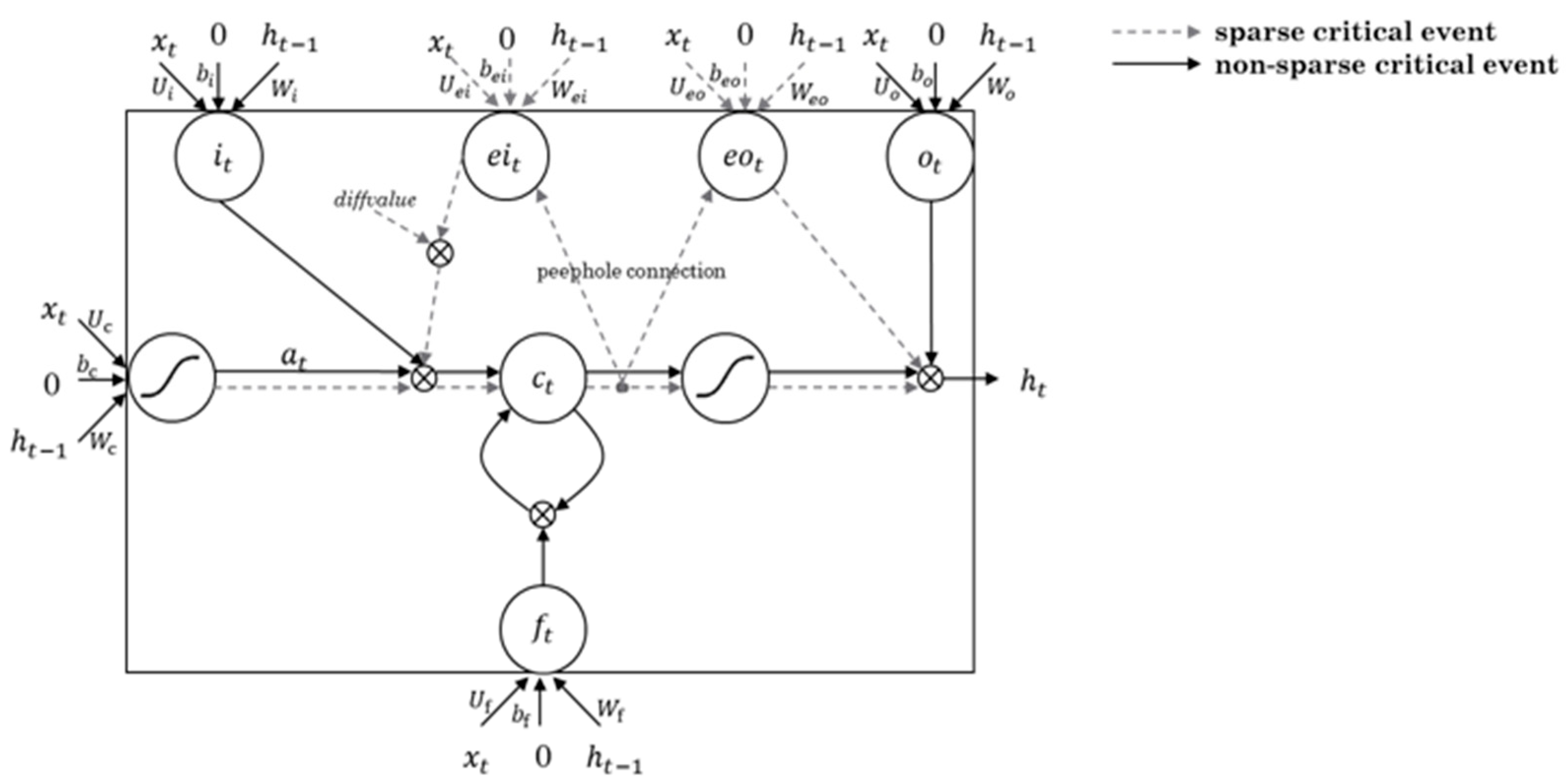
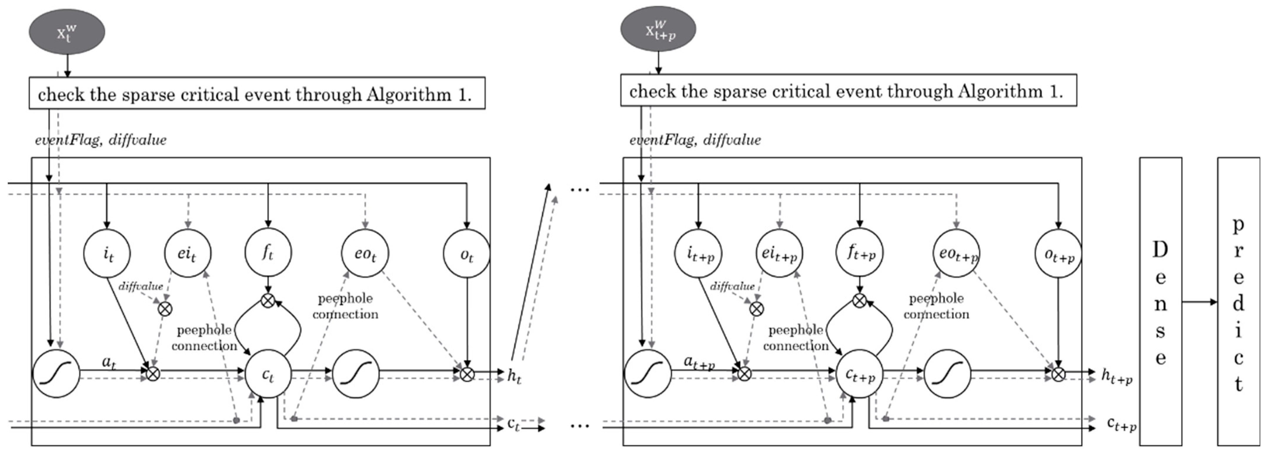
3.3. Designing SCE-LSTM Layer by Reflecting the SCE

The SCE-LSTM includes a modified layer that reflects SCE variables based on the mechanisms of selective attention and memorization of critical events in the human brain. The concept is implemented in the modified neural network model using a switch that prevents data being sent to the forget gate in the case of critical events. Furthermore, varying weights are assigned to the variables to ensure that the modified model can better mimic human brains in terms of selectively storing information with different weights in case of critical events [25,26,32,33]. Figure 3 shows the details of the proposed SCE-LSTM model.

As shown in Figure 3, the SCE-LSTM model includes a step to distinguish SCE from an input sequence and learn about critical and noncritical events, as described in Algorithm 2 (SCE-LSTM Cell$(Y,X,start\_index,d)$). Here, X refers to the input sequence of the entire data list to be learned and start_index refers to the first index of the window about d among the input sequences. Assuming that tensor X represents all information at time t, as described in the previous section, whether a sparse critical event occurs at time t is determined using Algorithm 1 (CheckSparseCriticalEvent $\left(Y,X,t,d\right)$ as step 1 in Algorithm 2. If it is not an SCE at that time, the learning method uses a conventional LSTM model directly, the flows of which are well represented by the solid lines in Figure 3.

Algorithm 2 CheckSparseCriticalEvent (Y, X, start_index, end_index)

Input (1)  $Y$: a time-series target sequence (2)  $X$: a time-series input sequence without UBB and LBB (3)  $d$: period to represent the number of continuous days (4)  $z$: weight for standard deviation of $p$

Output (5)  $X$: a time-series input sequence with calculated UBB and LBB values (6)  $diffValue$: sum of the difference of current target value and its previous one

Begin // $D$: a list to store the difference of current target value and its previous one // $C$: a list to store flags for representing whether a target value is critical // event: the number of critical events in $Y$ $D\leftarrow empty list$ $C\leftarrow empty list$ $event\leftarrow 0$ $diffValue\leftarrow 0$ $i\leftarrow$ start_index $\mathbf{w}\mathbf{h}\mathbf{i}\mathbf{l}\mathbf{e} i<end\_index \mathbf{d}\mathbf{o}$ $D\left[i\right]\leftarrow abs\left(Y\left[i+1\right]-Y\left[i\right]\right)$ $diffvalue\leftarrow diffValue+D\left[i\right]$ $\mathbf{i}\mathbf{f} X\left[i\right].ubb<Y\left[i\right] \mathbf{t}\mathbf{h}\mathbf{e}\mathbf{n}$ $C\left[i\right]\leftarrow 1$ $event\leftarrow event+1$ $\mathbf{e}\mathbf{l}\mathbf{s}\mathbf{e} Y\left[i\right]<X\left[i\right].lbb \mathbf{t}\mathbf{h}\mathbf{e}\mathbf{n}$ $C\left[i\right]\leftarrow 2$ $event\leftarrow event+1$ $\mathbf{e}\mathbf{l}\mathbf{s}\mathbf{e}$ $C\left[i\right]\leftarrow 0$ $i\leftarrow i+1$ end of while $eventFlag\leftarrow 0$ $\mathbf{i}\mathbf{f} event>0 \mathbf{t}\mathbf{h}\mathbf{e}\mathbf{n}$ $eventFlag\leftarrow 1$ $\mathbf{r}\mathbf{e}\mathbf{t}\mathbf{u}\mathbf{r}\mathbf{n} eventFlag, diffValue$

The conventional LSTM model is processed through from Step 2.1 to Step 2.8 in Algorithm 2 using the following equations [34].

The conventional LSTM model first receives $h_{t-1}$ and $X_t$ using Equation (3), calculates a forget gate, and sends a value of 0 or 1 to $c_{t-1}$. If the resulting value is one, the value will be preserved; if it is zero, the value will be discarded.

$$f_t\leftarrow \sigma \left(U_f{X}_t+W_f{h}_{t-1}+b_f\right)$$

(3)

An input gate is calculated after $h_{t-1}$ and $X_t$ are received through Equations (4) and (5). Then, it is determined whether the value of the cell state is to be updated through $a_t$ according to the resulting value of the forget gate.

$$i_t\leftarrow \sigma \left(U_i{X}_t+W_i{h}_{t-1}+b_i\right)$$

(4)

$$a_t\leftarrow \tanh \left(U_c{X}_t+W_c{h}_{t-1}+b_c\right)$$

(5)

Subsequently, the past cell state is updated according to the resulting value of what to forget and what to update from Equations (3)–(5). In Equation (6), the forget gate $f_t$ is multiplied by the past cell state $c_{t-1}$, and $i_t$ is multiplied by $a_t$ so that the data to be forgotten reach zero through multiplication, and those to be remembered are recorded using addition.

$$ct\leftarrow it°at+ft°ct-1$$

(6)

The following step is to determine what to report as output by calculating the output gate $o_t$ of Equation (7) and by multiplying $o_t$ with a specific part of the cell state $c_t$ in Equation (8). Finally, the output $h_t$, is reported.

$$o_t\leftarrow \sigma (U_o{X}_t+W_o{h}_{t-1}+b_o)$$

(7)

$$h_t\leftarrow o_t°\mathrm{t}\mathrm{a}\mathrm{n}\mathrm{h} \left(c_t\right)$$

(8)

Conversely, if it is a SCE at the time, the learning method does not pass the representative forget gate in the LSTM model, as indicated by the dotted lines in Figure 3.

In the case of a sequence determined as an SCE, the event input gate is calculated by receiving $h_{t-1}$ and $X_t$ using Equations (9) and (10). At this time, to reflect the cell state in the gate when calculating the event input gate in Equation (9), a peephole connection, which is a modified LSTM model introduced by [35], is added to reflect the past cell state value in the event input gate.

$${ei}_t\leftarrow \sigma \left(U_{ei}{X}_t+W_{ei}{h}_{t-1}+W_{ei}{c}_{t-1}+b_{ei}\right)$$

(9)

$$a_t\leftarrow \mathrm{t}\mathrm{a}\mathrm{n}\mathrm{h} (U_c{X}_t+W_c{h}_{t-1}+b_c)$$

(10)

The past cell state is updated according to the resulting value of the event input sequence calculated in steps Equations (9) and (10). The calculation is performed by multiplying ${ei}_t$ by the weight of the SCE, i.e., the product of diffValue, as shown in Equation (11), and the events to be recorded as SCE, i.e., $a_t$. Subsequently, the current cell state $c_t$ is calculated by adding $c_{t-1}$ to the updated past cell state.

$$c_t\leftarrow ({ei}_t{°diffValue)°a}_t+c_{t-1}$$

(11)

Finally, the output is determined by calculating the event output gate $e{o}_t$ in Equation (12). Similarly, by adding a peephole connection, it is calculated by reflecting the $c_t$ state of the previously calculated cell state. Subsequently, a specific part of the cell state $c_t$ and ${eo}_t$ is calculated using Equation (13), and the output, $h_t$, is reported.

$${eo}_t\leftarrow \sigma \left(U_{eo}{x}_t+W_{eo}{h}_{t-1}+W_{eo}{c}_t+b_{eo}\right)$$

(12)

$$h_t\leftarrow {eo}_t°\mathrm{t}\mathrm{a}\mathrm{n}\mathrm{h} \left(c_t\right)$$

(13)

The algorithm for calculating SCE-LSTM cells using Equations (3)–(13) is detailed in Algorithm 3. Specifically, the data-learning method using the SCE-LSTM cell is presented in Algorithm 3, where X refers to a list of input sequences to be learned, $p$ refers to the number of data in a window, $d$ refers to the number of input sequences in a given duration to find an SCE, and $pred\_m$ refers to the number of predicted values to be estimated after learning. When the total number of data points is n, the number of windows can be calculated as $wdn=n-p+1$. The overall configuration diagram for the SCE-LSTM layer using the SCE-LSTM cell, i.e., the proposed model for learning the SCE, is shown in Figure 4.

When $x_t^{wdi}$ refers to the input sequence at the start time $t$ of the i-th window ${wd}_i$, the i-th window is from $x_t^{{wd}_i}$ to $x_{t+p}^{{wd}_i}$ at the point of $t+p$. Data from the window are used for the SCE-LSTM cell to learn, as described in Algorithm 2. For each input, $eventFlag \mathrm{a}\mathrm{n}\mathrm{d} diffValue$ is calculated using the Check SparseCriticalEvent function of Algorithm 1, and the SCE-LSTM cell function of Algorithm 2 is used to learn the input sequence. The learning process is repeated until the last input sequence, $x_{t+p}^{{wd}_i}$, and the prediction sequence is created through the dense layer.

Algorithm 3 SCE-LSTM Cell (Y, X, start_index, d)

Input (1)  $Y$: a time-series target sequence $Y$: a time-series target sequence (2)  $X$: a time-series input sequence with calculated UBB and LBB values (3)  $start\_index$: the first index of window (4)  $d$: the number of data in window

Output (5)  $h_t$: LSTM output (6)  $c_t$: Cell State output

Begin //$U_f,U_i,U_c,U_o,U_{ei},U_{eo}$: Weight values for $X_t$ //$W_f,W_i,W_c,W_o,W_{ei},W_{eo}$: Weight values for $h_{t-1}$   $eventValue, diffValue\leftarrow \mathrm{C}\mathrm{h}\mathrm{e}\mathrm{c}\mathrm{k}\mathrm{S}\mathrm{p}\mathrm{a}\mathrm{r}\mathrm{s}\mathrm{e}\mathrm{C}\mathrm{r}\mathrm{i}\mathrm{t}\mathrm{i}\mathrm{c}\mathrm{a}\mathrm{l}\mathrm{E}\mathrm{v}\mathrm{e}\mathrm{n}\mathrm{t}\left(Y, X, start\_index, start\_index+d\right)$ $\mathbf{i}\mathbf{f} eventFlag==0 \mathbf{t}\mathbf{h}\mathbf{e}\mathbf{n}$ for t$=start\_idex$ to $t<star{t}_{index}+d;$ $t=t+1$ do ${\hspace{1em}\hspace{0.33em}f}_t\leftarrow \sigma \left(U_f{X}_t+W_f{h}_{t-1}+b_f\right)$ $i_t\leftarrow \sigma \left(U_i{X}_t+W_i{h}_{t-1}+b_i\right)$ ${\hspace{1em}a}_t\leftarrow \mathrm{t}\mathrm{a}\mathrm{n}\mathrm{h} (U_c{X}_t+W_c{h}_{t-1}+b_c)$ $c_t\leftarrow i_t°a_t+f_t°c_{t-1}$ $o_t\leftarrow \sigma \left(U_o{X}_t+W_o{h}_{t-1}+b_o\right)$ $h_t\leftarrow o_t°\mathrm{t}\mathrm{a}\mathrm{n}\mathrm{h} \left(c_t\right)$ End for $\mathbf{e}\mathbf{l}\mathbf{s}\mathbf{e} eventFlag==1 \mathbf{t}\mathbf{h}\mathbf{e}\mathbf{n}$ for t$=start\_idex$ to $t<start\_index+d; t=t+1$ do ${ei}_t\leftarrow \sigma \left(U_{ei}{X}_t+W_{ei}{h}_{t-1}+W_{ei}{c}_{t-1}+b_{ei}\right)$ $a_t\leftarrow \tanh \left(U_c{X}_t+W_c{h}_{t-1}+b_c\right)$ $c_t\leftarrow ({ei}_t{°diffValue)°ea}_t+c_{t-1}$ ${eo}_t\leftarrow \sigma \left(U_{eo}{X}_t+W_{eo}{h}_{t-1}+W_{eo}{c}_t+b_{eo}\right)$ $h_t\leftarrow {eo}_t°\tanh \left(c_t\right)$ End for $\mathbf{r}\mathbf{e}\mathbf{t}\mathbf{u}\mathbf{r}\mathbf{n} h_t, c_t$

Following the input sequence, the Algorithm 4 SCE-LSTM model is created using the SCE-LSTM cell according to Algorithm 3 and the predicted result value, $predict\_result$, is returned. The learning of the input sequence is window-based, and the number of windows is calculated based on the length of the input sequence $X$, and the number of data points in window $p$. The window was utilized to increase the accuracy of the model by repeatedly learning the SCE in the input sequence for each window. Following the estimation of the number of windows, the input sequence $X$, window start index $t$, and the number of data in window $p$ are transmitted to the SCE-LSTM cell. Then, via CheckSparseCriticalEvent in Algorithm 1, $eventFlag$, which determines whether there is a critical event in the corresponding window input sequence, and $diffValue$, which is the result of adding the difference between the next and previous days of the window, are calculated in Algorithm 2. When the value of $eventFlag$ is zero, the input sequence of the corresponding window is considered as a non-sparse critical event and learned through the conventional LSTM learning method of Equations (3)–(8). When the value of $eventFlag$ is 1, the input sequence of the corresponding window is considered to include an SCE and is learned using Equations (9)–(13). The learned model returns the cell state value, $c_t$, and output value of the hidden layer, $h_t$. The proposed model repeats learning as many times as the number of windows and finally generates the prediction through the dense layers, which amounts to pred_m values.

Algorithm 4 SCE-LSTM model (Y, X, p, d, pred_m)

Input (1)  $Y$: a time-series target sequence (2)  $X$: a time-series input sequence with calculated UBB and LBB values. (3)  $p$: the number of data in a window (4)  $d$: the number of input sequences in a considered duration once (5)  $pred\_m$: the number of predicted values

Output (6)  $predict$_result: predicted result for $pred\_m$ using proposed SCE-LSTM

Begin $n\leftarrow x.length$ $W\leftarrow n-p+1$ $w\leftarrow 0$ $t\leftarrow 0$ $n\leftarrow x.length$ $W\leftarrow n-p+1$ $w\leftarrow 0$ $t\leftarrow 0$ $w\leftarrow w+1$ end of while $predict\_result\leftarrow dense(pred\_m)$ return $predict\_result$

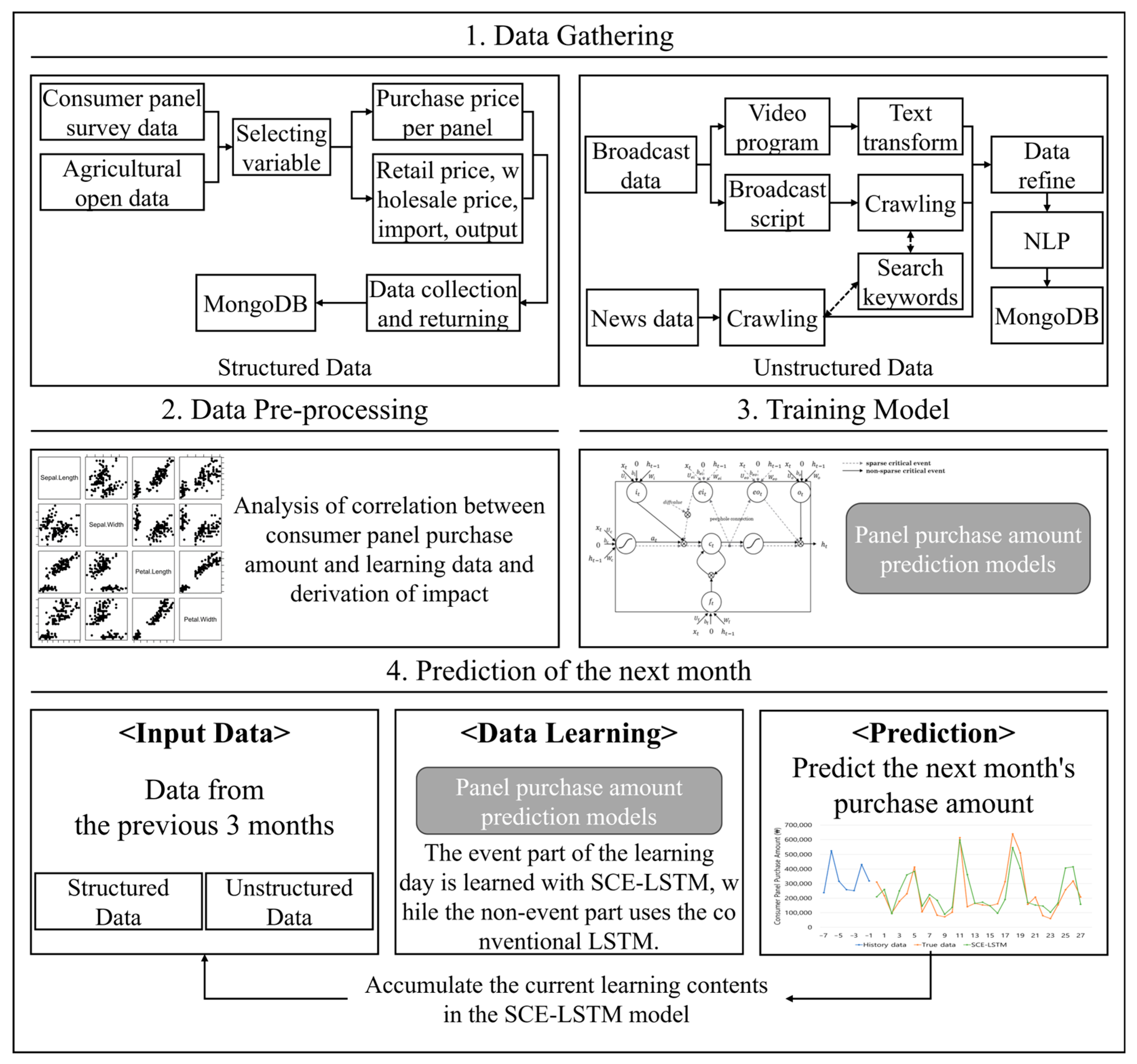
4. Predicting the Purchase Amount of Pork Meat Using the Proposed SCE-LSTM

In this section, we describe how the proposed SCE-LSTM can be applied to predict the daily amounts of money spent to purchase pork belly meat under the influence of a few critical events. In Section 4.1, we describe data collection and pre-processing. Subsequently, in Section 4.2, we describe how the SCE-LSTM was used to estimate the daily amount of money spent to purchase pork belly meat for the next pred_m = 30 days using Algorithm 4 in Section 3.3.

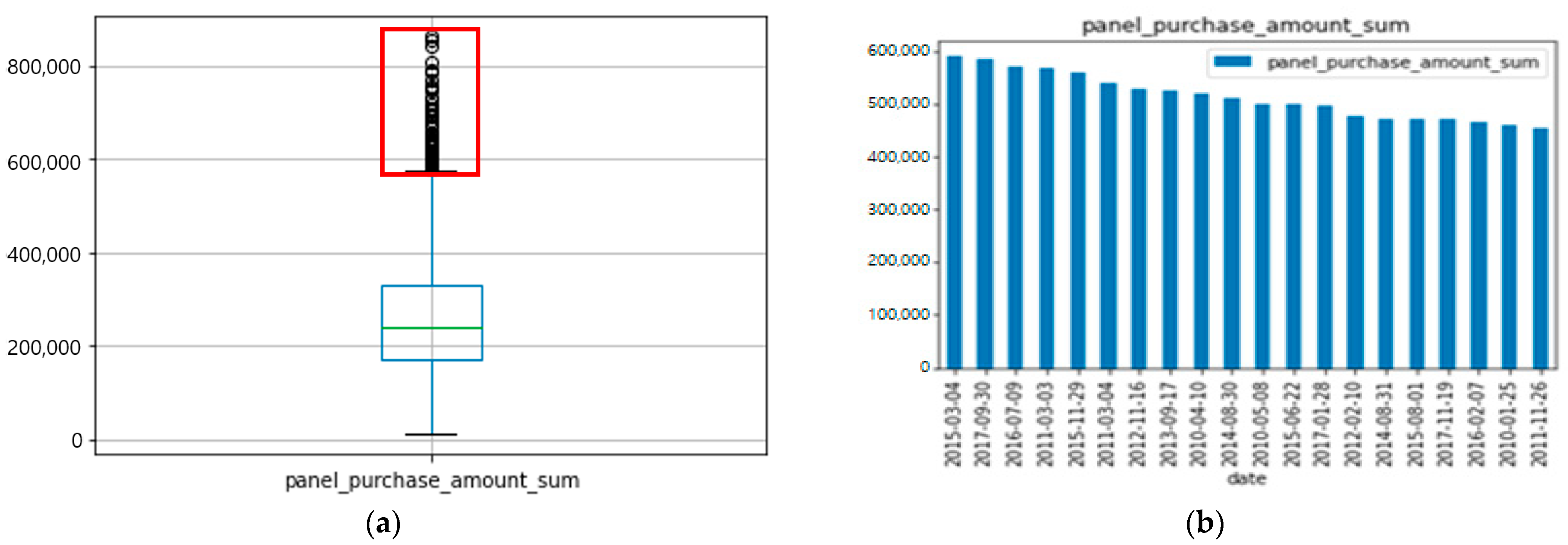
4.1. Data Collection and Pre-Processing

The target variable is the daily amount of money spent to purchase pork belly meat from 2010 to 2017. The independent variables in the same period as the target variable comprise 8 structured and 19 unstructured data, which can affect the daily amounts of money spent, as listed in

Table 2. Independent variables of structured data used in this study.

Column	Description
retail_price_meat	Daily retail prices of pork belly meat
wholesale_price_carcass	Daily wholesale prices of pork carcass
pig_bred_number_quarter_before	Number of pigs bred in previous quarter
pig_slaughtered_number_quarter_before	Number of pigs slaughtered in previous quarter
wholesale_price_carcass_quarter_before	Daily wholesale prices of pork carcass in previous quarter
output_ton_year_before_carcass	Pork meat production in previous year (ton)
import_ton_year_before	Imported pork meat in previous year (ton)
monthly_sales_trend_ton_meat	Monthly sales trend of pork meat (ton)

and

Table 3. Independent variables of unstructured data used in this study.

Column	Description	Record Numbers
news_freq	Frequency of the appearance of the word in pig news contents	6655
emotions_number_angries	Frequency of sentiment for news content	3979
emotion_number_likes		14,811
emotions_number_sads		395
emotions_number_wants		438
emotions_number_warms		153
news_comment_freq	Frequency of the appearance of the word in pig news comment	44,342
news_positive_term_freq	Frequency of positive word appearance in pig news content	35,319
news_negative_term_freq	Frequency of negative word appearance in pig news content	4429
video_freq	Frequency of the appearance of the word in pig TV programs	1529
video_total_ranking_ave_p	Video total ranking average	1529
video_freq_times_viewrate	Video frequency times view rate	1529
video_positive_term_freq	Frequency of positive word appearance in pig TV programs content	119,396
video_negative_term_freq	Frequency of negative word appearance in pig TV programs content	4745
blog_freq	Frequency of the appearance of the word in pig blog	75,035
blog_comments	Frequency of word appearance in a pig blog comment	109,950
blog_likes	Frequency of sentiment for blog content	70,025
blog_positive_term_freq	Frequency of positive word appearance in pig blog content	1,666,492
blog_negative_term_freq	Frequency of negative word appearance in pig blog content	56,870

. The structured data comprise factors related to consumption, such as retail price, wholesale price, sales quantity, and import volume (Table 2). The structured data were collected using open API and include wholesale market data from the Outlook and Agricultural Statistics Information System (OASIS) of the Korea Rural Economic Institute, retail Service (KAMIS), and pork production data from the Korean Statistical Information System (KOSIS) [36]. Because the data period for each element was different, all raw data were pre-processed daily. The unstructured data used in this study were collected from news (e.g., “news freq”, “emotions number angries”, “emotion number likes”, “emotions number sads”, “emotions number wants”, “emotions number warms”, “news comment freq”, “news positive term freq”, and “news negative term freq”), broadcast video programs (e.g., “video freq, video total ranking ave p”, “video freq times viewrate”, “video positive term freq”, and video negative term freq”), and blogs (e.g., “blog freq”, “blog comments”, “blog likes”, “blog positive term freq”, and “blog negative term freq”), as shown in Table 3. The collected unstructured data include dates, titles and whole text, frequency of terms of interest mentioned in the text (e.g., a term “pork belly meat”), positive/negative words in the text, and frequency of these positive/negative words. Words in the text were classified as positive (e.g., delicious), neutral (e.g., really), or negative (e.g., nasty) according to the part of speech to which the word belonged.

4.2. Application of the Proposed SCE-LSTM

To create a consumption prediction model for agricultural/livestock products that can reflect SCE, the proposed SCE-LSTM model Section 3.2 is applied. The structured and unstructured data used for analysis are for the consumption prediction of pork belly meat in Korea, and they are listed in Table 2 and Table 3 from Section 4.1. The collected data were pre-processed through data normalization and correlation analysis. Data normalization of independent and dependent variables includes min–max scaling, converting data into values between 0 and 1 to normalize the data distribution. Correlation analysis was used to estimate weights for the normalized data by deriving the correlation with the target value, i.e., the daily amount of money spent to purchase pork belly meat. After data normalization of the independent variables, a consumption prediction learning model was created using the proposed SCE sequence detection and learning method of the SCE-LSTM. For the prediction of pork belly meat consumption, the prediction model was trained with the consumption data for 3 months, and consumption for a period of one month was predicted. The model continually accumulated the learning content based on the window. The min–max normalization was calculated using the following formula:

$$x^{\prime }=\frac{\left(x-\mathit{min}\left(x\right)\right)}{\mathit{max}\left(x\right)-\mathit{min}\left(x\right)+1e-7}$$

(14)

An overall diagram of the proposed SCE-LSTM application is shown in Figure 5.

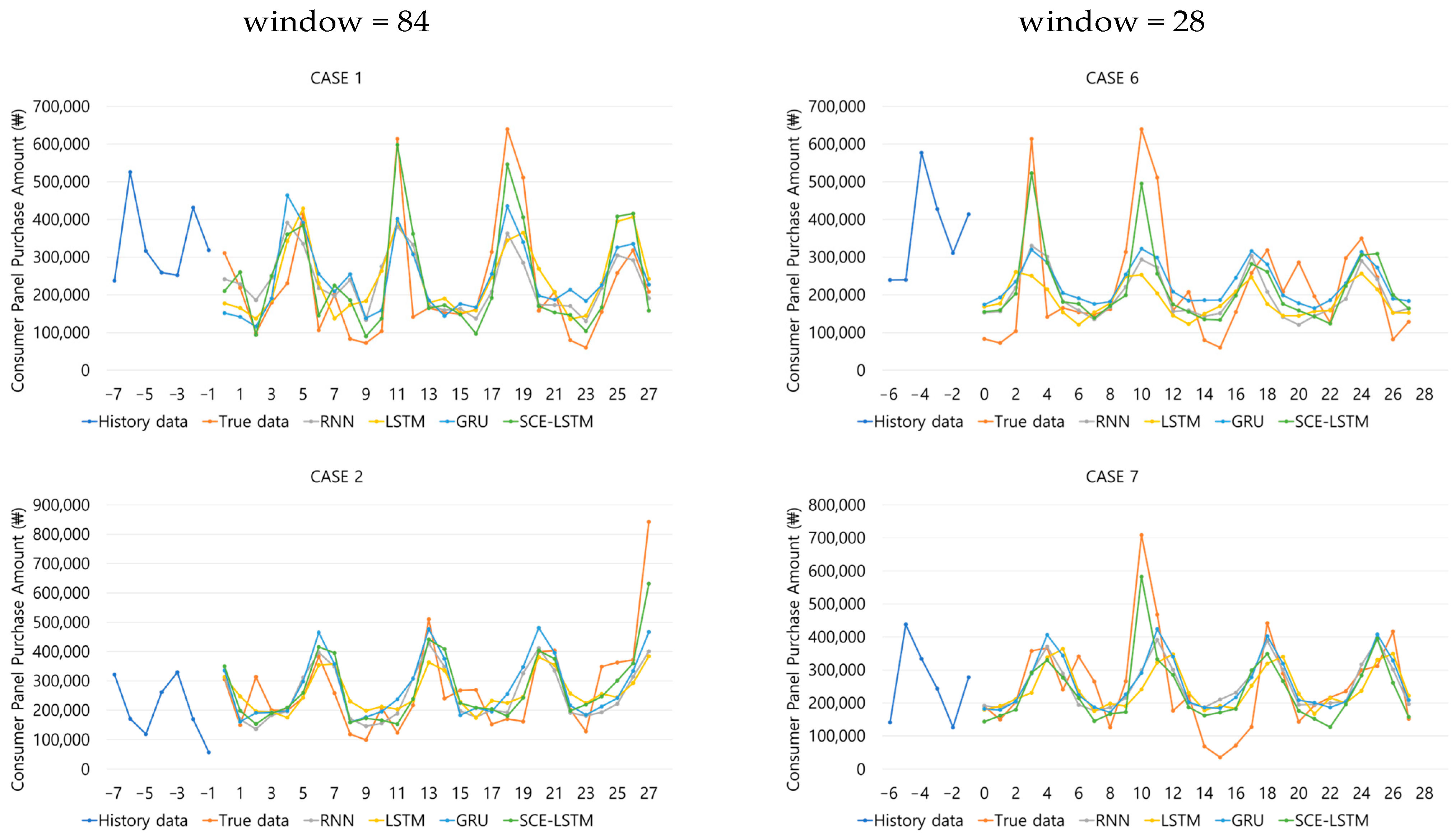
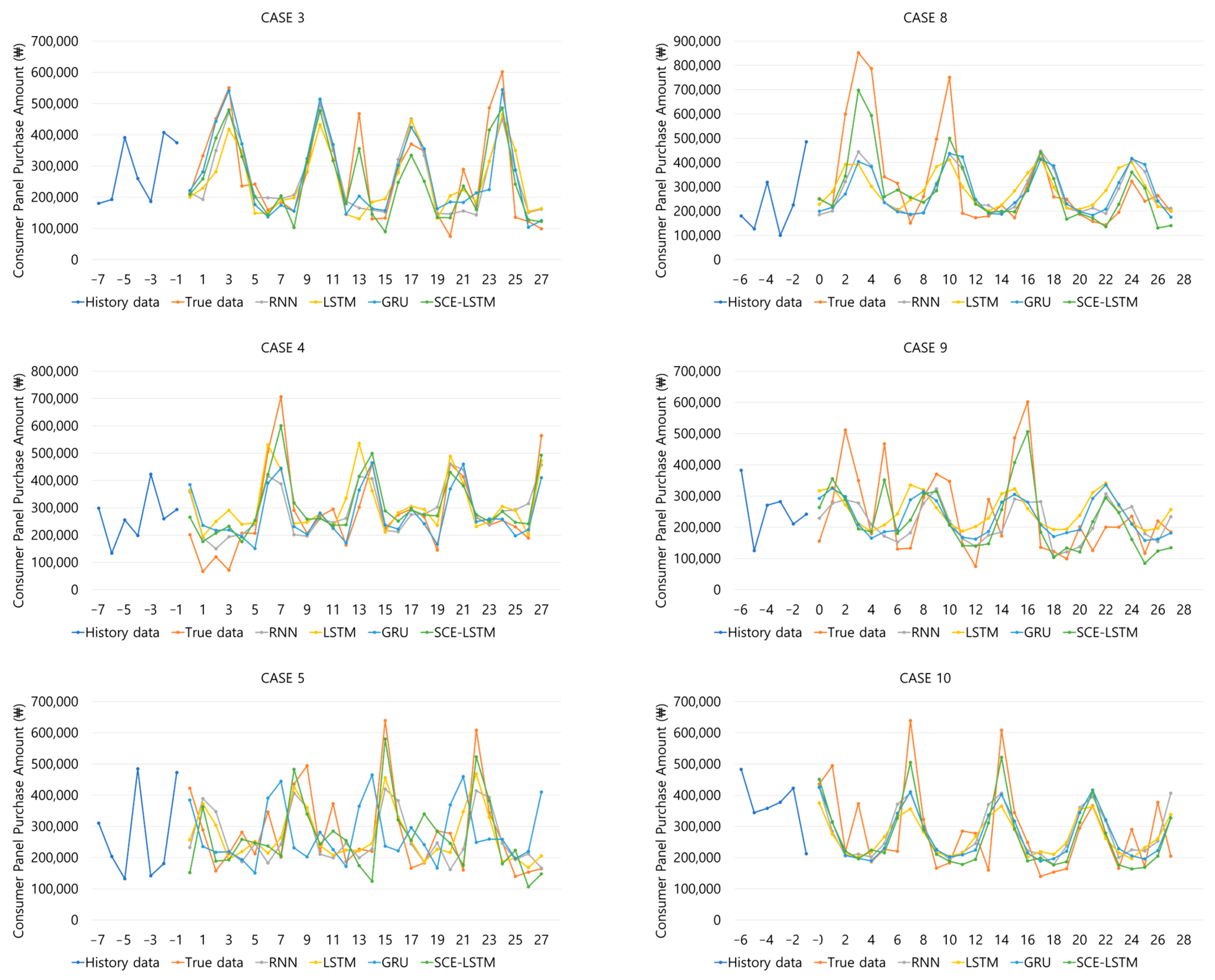
5. Performance Evaluation

In this section, we describe how different time-series deep learning models, such as RNN, LSTM, and GRU, in addition to the proposed SCE-LSTM, were evaluated for their prediction performances. In Section 5.1, we describe the experimental setup and evaluation models, followed by the evaluation metrics in Section 5.2, and the model hyperparameters and experimental results in Section 5.3.

5.1. Experimental Models

When using a conventional neural network to predict various types of data, continuous information is difficult to store. To address this problem, RNN learning models, which are advanced Neural Network models, have been commonly used to learn sequential data [2]. An RNN model repeats itself and retains the information obtained in the previous step. Moreover, in contrast to conventional neural networks, it can retain data. The chain-based RNN model, in particular, has been optimized for dealing with sequenced data and is frequently used in various fields, including speech recognition and language modeling.

However, long-term dependencies are a central problem; RNNs forget information over time [36,37]. To solve this problem, LSTM, which learns information while controlling the cell state through the cell state and input, forget, and output gates, was introduced [14]. In the first step of LSTM, the forget gate, which determines which information is to be discarded from the cell state, outputs a value between 0 and 1 through a sigmoid operation. If the forget gate has a value of one, all information is preserved; if it has a value of zero, all information disappears. The second step is to determine which of the new information is to be stored in the cell state in the future. During this step, a vector of new candidate values is created through a hyperbolic tangent operation to determine the value that is to be updated through the sigmoid operation of the input gate. The information is subsequently merged into the cell state to create information to be updated. The third step is to update the old cell state to create a new cell state. New information is added to the new cell state by multiplying the value from the input gate by the vector of candidate values. This added value becomes a scaled value of the updated information from the input gate. Finally, based on the cell state, the output gate value is calculated to output the filtered value. In this step, the value of the output gate is calculated using a sigmoid function to determine which part of the cell state to output as input information. The cell state subsequently receives a value between −1 and 1 through a hyperbolic tangent operation, and that value is multiplied by the value of the output gate. Consequently, only the desired part is exported from the input information to the output gate. There is a modified LSTM model, the peephole LSTM, which learns by considering the cell state for each gate of the LSTM [35]. Although this method considers the previous cell state, it is incapable of reflecting the SCE value. Another modified LSTM model, the GRU model, was introduced to compensate for the heavy use of weights in the LSTM model [38]. This model combines the forget gate and input gate into an update gate and learns the data after combining the cell and hidden states.

5.2. Evaluation Metrics

The model’s performance in predicting daily amounts of money spent to purchase pork belly meat were evaluated by comparing predicted amounts with actual amounts in terms of error rates, including root mean squared error (RMSE), mean absolute error (MAE), MAPE, and mean percentage error (MPE).

Among the error rates used, the MSE of the RMSE is the mean squared difference between the actual and predicted values and is the sum of the area of the difference between the predicted and the actual values. A characteristic of the MSE is that its value increases with the presence of outliers. In addition, since MSE calculates the square of the error, its error rate tends to be larger than actual error rates; thus, RMSE values, i.e., the root of the MSE values, are used instead. MAE is obtained by converting the differences between the actual and predicted values into an absolute value and then averaging it. Since MAE considers the absolute value errors, the size of an error is reflected as it is, and it has the advantage of being less affected by outliers. MAPE is the conversion of MAE to a percentage and also has the advantage of being less affected by outliers. However, because MAE and MAPE take absolute values, the model’s performance, i.e., whether it predicts higher values (overperformance) or lower values (underperformance) than the actual values, is unclear. Therefore, the accuracy of the MAE and MAPE values should be confirmed using the MPE. MPE is an index that excludes absolute values from MAPE and determines whether a model shows overperformance (−) or underperformance (+).

Table 4. Comparison of the error rates for each case using the proposed model.

Test Case	Parameter				Error Rate
	Window	Batch Size	Epoch	$\mathbf{Whether} \mathbf{to} \mathbf{Use} \mathit{d}\mathit{i}\mathit{f}\mathit{f}\mathit{V}\mathit{a}\mathit{l}\mathit{u}\mathit{e}$ in Event Sequence	RMSE	MAE	MAPE	MPE
1	84	64	500	Used	0.11	0.09	35.48	−6.60
				Not used	0.16	0.12	49.09	−17.50
2	84	64	300	Used	0.08	0.06	23.80	−3.17
				Not used	0.13	0.10	36.44	−9.36
3	28	64	500	Used	0.14	0.11	48.70	−20.65
				Not used	0.15	0.13	61.83	−39.95
4	28	64	300	Used	0.14	0.11	50.25	−24.68
				Not used	0.14	0.11	41.58	−2.44
5	84	32	500	Used	0.09	0.08	32.61	−11.56
				Not used	0.10	0.08	33.49	−13.64
6	84	32	300	Used	0.09	0.07	30.87	−12.52
				Not used	0.10	0.08	33.90	−13.86
7	28	32	500	Used	0.16	0.12	66.33	−45.59
				Not used	0.16	0.12	64.31	−39.60
8	28	32	300	Used	0.16	0.12	72.91	−57.40
				Not used	0.15	0.12	70.66	−52.69

presents a comparison of the error rates for each case in the proposed model. After comparing error rates according to window, batch size, epoch, and whether diffValue was used, the result obtained using diffValue in case2 was found to exhibit the lowest error rate. The error rate metrics are defined as follows:

$$RMSE=\sqrt{\frac{1}{N}\sum _{i=1}^N{\left(y_i-f_i\right)}^2}$$

(15)

$$MAE=\frac{1}{N}\sum _{i=1}^N|y_i-f_i|$$

(16)

$$MAPE=\frac{1}{N}\sum _{i=1}^N\frac{|y_i-f_i|}{y_i}$$

(17)

$$MPE=\frac{1}{N}\sum _{i=1}^N\frac{(y_i-f_i)}{y_i}$$

(18)

5.3. Model Hyperparameters and Experimental Results

In this study, agricultural data were compared using the SCE-LSTM method proposed in Section 3.3 and the deep learning-based time-series prediction methods described in Section 5.1. The proposed SCE-LSTM method can provide accurate predictions, even in a sequence with rapid changes. Therefore, to confirm its effectiveness, we identified and predicted the cases with SCE and compared the error rate. The model performances were compared by calculating the RMSE, MAE, MAPE, and MPE according to the window for the RNN, LSTM, GRU, and the proposed method, SCE-LSTM. For this comparison, the parameter settings were identical for all the methods, i.e., the batch size was 64 and the epoch was 300. Thus, we can see how well the most accurate method performed in the same setting as the learning methods, how well SCE were found, and how well SCE sequences were predicted.

Table 5. Comparison of error rates among different learning methods according to window values for 10 test cases of SCE.

Test Case	Method	Window	RMSE	MAE	MAPE	MPE	Parameter
1	RNN	84	0.13	0.10	57.70	−39.19	batch size = 64 epoch = 300
	LSTM		0.13	0.10	57.46	−40.22
	GRU		0.12	0.09	59.63	−42.88
	SCE-LSTM		0.11	0.09	45.93	−25.97
2	RNN	84	0.13	0.09	32.18	−6.83	batch size = 64 epoch = 300
	LSTM		0.13	0.09	36.26	−14.83
	GRU		0.12	0.09	34.64	−16.95
	SCE-LSTM		0.11	0.07	27.60	−10.67
3	RNN	84	0.11	0.08	30.45	−8.98	batch size = 64 epoch = 300
	LSTM		0.12	0.09	37.70	−11.70
	GRU		0.10	0.06	28.12	−9.04
	SCE-LSTM		0.08	0.06	22.55	1.95
4	RNN	84	0.11	0.08	38.96	−25.21	batch size = 64 epoch = 300
	LSTM		0.12	0.08	48.46	−38.02
	GRU		0.10	0.07	38.43	−20.91
	SCE-LSTM		0.10	0.07	37.95	−20.83
5	RNN	84	0.12	0.09	29.12	−3.69	batch size = 64 epoch = 300
	LSTM		0.10	0.08	28.93	−6.34
	GRU		0.10	0.08	27.29	−10.96
	SCE-LSTM		0.10	0.07	26.20	0.15
6	RNN	28	0.14	0.10	51.00	−20.08	batch size = 64 epoch = 300
	LSTM		0.16	0.11	55.67	−19.22
	GRU		0.13	0.10	62.31	−42.22
	SCE-LSTM		0.13	0.09	49.21	−22.41
7	RNN	28	0.13	0.09	66.53	−47.47	batch size = 64 epoch = 300
	LSTM		0.14	0.10	65.99	−41.44
	GRU		0.13	0.09	63.28	−45.50
	SCE-LSTM		0.13	0.10	59.76	−27.30
8	RNN	28	0.18	0.12	32.07	−2.84	batch size = 64 epoch = 300
	LSTM		0.19	0.12	34.93	−10.59
	GRU		0.19	0.13	34.42	−3.81
	SCE-LSTM		0.16	0.10	26.33	2.30
9	RNN	28	0.13	0.09	37.33	−8.35	batch size = 64 epoch = 300
	LSTM		0.16	0.13	61.00	−35.89
	GRU		0.15	0.11	50.19	−21.95
	SCE-LSTM		0.14	0.11	41.58	−2.44
10	RNN	28	0.12	0.09	32.26	−11.04	batch size = 64 epoch = 300
	LSTM		0.13	0.09	32.55	−7.99
	GRU		0.11	0.09	29.32	−6.81
	SCE-LSTM		0.11	0.08	26.94	−0.18

shows the results of comparing the error rates for the learning methods according to the window values for 10 test cases of SCE. Figure 5 shows the MAPE results in Table 5 for the SCE case. Figure 5 shows that SCE-LSTM has the lowest error rates compared with the other prediction methods in all cases except Case 9, in which RNN has the lowest error rate. However, the MPE of SCE-LSTM in Case 9 indicates that the predicted values of SCE-LSTM are closer to the actual values than those of the other methods (Table 5).

In Figure 6, a window of 84 is used for the model parameters of Cases 1–5, whereas a window of 28 is used for Cases 6–10. In Case 1 of Figure 6, SCE-LSTM exhibits the lowest error rates and predicts the 11th and 18th values closest to the actual data. In Case 2, the error rate is the lowest in SCE-LSTM, and the 27th value of SCE-LSTM is closest to the actual data. In Case 4, RMSE and MAE values of SCE-LSTM and GRU are identical in Table 5; however, the MAPE and MPE values are lower in SCE-LSTM than in GRU. Case 4 indicates similar error rates between the SCE-LSTM and GRU; however, the 7th and 27th values of the SCE-LSTM are closest to the actual data. In Case 5, the RMSE values of LSTM, GRU, and SCE-LSTM are identical, as shown in Table 5; nevertheless, the 15th and 22nd values by SCE-LSTM are the closest to the actual data. In Cases 6 to 10, SCE-LSTM predicts the SCE values more accurately than the other predictive methods. However, in Case 9, the error rates are lowest in the RNN, as shown in Table 5. Nevertheless, the predicted results indicate that the 15th and 16th values of the SCE-LSTM are closest to the actual data. The detailed visualization of all test cases is presented in Figure 7.

6. Conclusions

In this study, we introduced the SCE-LSTM method, which is designed to emulate human memory’s selective attention and memorization of critical events. This innovative approach excels at identifying sparse critical event (SCE) sequences during data learning, effectively dividing data into cases involving sparse and non-sparse critical events. In stark contrast, conventional LSTM struggles to learn SCE sequences due to the constraints of its forget gate and input vector computations within the cell state. SCE-LSTM, during data learning, bypasses the forget gate for SCE sequences and estimates weight values as differences in the input vector, ensuring that the updated portion of the SCE’s input candidate vector can contribute more substantially to the cell state. In the case of non-sparse critical events, sequences are learned through conventional LSTM.

Our application of the proposed SCE-LSTM method to predict agricultural time-series data, characterized by rapid fluctuations, yielded promising results. We conducted a comparative analysis with other deep learning-based models, including RNN, LSTM, and GRU. The outcomes underscore the superior predictive accuracy of SCE-LSTM, closely aligning with actual daily expenditures on purchasing pork belly and exhibiting the lowest error rates among the models tested.

While our study demonstrates the efficacy of the proposed approach among the compared deep learning models, there remains room for improving the prediction accuracy. Future investigations should delve into SCE identification and the incorporation of additional indicators representing diverse trends. Additionally, understanding the optimal duration for retaining sparse critical event sequences with varying weights presents a significant avenue for further research.

In conclusion, the SCE-LSTM model represents a valuable advancement in predicting agricultural consumption, particularly during unforeseen critical events like livestock epidemics, such as African swine fever, that impact the market. Its potential for enhancing predictive accuracy is evident, and ongoing research endeavors in this direction are poised to contribute to more robust and reliable forecasting methods in the field.

References

1. Neves, R.F.L. An Overview of Deep Learning Strategies for Time Series Prediction. Master’s Thesis, Instituto Superior Técnico, Lisboa, Portugal, 2018. [Google Scholar]
2. Grossberg, S. Recurrent neural networks. Scholarpedia 2013, 8, 1888. [Google Scholar] [CrossRef]
3. Li, Q.; Tan, J.; Wang, J.; Chen, H. A multimodal event-driven lstm model for stock prediction using online news. IEEE Trans. Knowl. Data Eng. 2020, 33, 3323–3337. [Google Scholar] [CrossRef]
4. Lin, H.; Sun, Q. Crude oil prices forecasting: An approach of using CEEMDAN-based multi-layer gated recurrent unit networks. Energies 2020, 13, 1543. [Google Scholar] [CrossRef]
5. Long, W.; Lu, Z.; Cui, L. Deep learning-based feature engineering for stock price movement prediction. Knowl.-Based Syst. 2019, 164, 163–173. [Google Scholar] [CrossRef]
6. Ozbayoglu, A.M.; Gudelek, M.U.; Sezer, O.B. Deep learning for financial applications: A survey. Appl. Soft Comput. 2020, 93, 106384. [Google Scholar] [CrossRef]
7. Wen, M.; Li, P.; Zhang, L.; Chen, Y. Stock market trend prediction using high-order information of time series. IEEE Access 2019, 7, 28299–28308. [Google Scholar] [CrossRef]
8. Chuluunsaikhan, T.; Ryu, G.-A.; Yoo, K.-H.; Rah, H.; Nasridinov, A. Incorporating deep learning and news topic modeling for forecasting pork prices: The case of South Korea. Agriculture 2020, 10, 513. [Google Scholar] [CrossRef]
9. Ryu, G.-A.; Nasridinov, A.; Rah, H.; Yoo, K.-H. Forecasts of the amount purchase pork meat by using structured and unstructured big data. Agriculture 2020, 10, 21. [Google Scholar] [CrossRef]
10. Yoo, T.-W.; Oh, I.-S. Time series forecasting of agricultural products’ sales volumes based on seasonal long short-term memory. Appl. Sci. 2020, 10, 8169. [Google Scholar] [CrossRef]
11. Chung, J.; Gulcehre, C.; Cho, K.; Bengio, Y. Empirical evaluation of gated recurrent neural networks on sequence modeling. arXiv 2014, arXiv:1412.3555. [Google Scholar]
12. Li, Q.; Chen, Y.; Jiang, L.L.; Li, P.; Chen, H. A tensor-based information framework for predicting the stock market. ACM Trans. Inf. Syst. (TOIS) 2016, 34, 1–30. [Google Scholar] [CrossRef]
13. Sun, T.; Wang, J.; Zhang, P.; Cao, Y.; Liu, B.; Wang, D. Predicting stock price returns using microblog sentiment for chinese stock market. In Proceedings of the 2017 3rd International Conference on Big Data Computing and Communications (BIGCOM), Chengdu, China, 10–11 August 2017; pp. 87–96. [Google Scholar]
14. Hochreiter, S.; Schmidhuber, J. Long short-term memory. Neural Comput. 1997, 9, 1735–1780. [Google Scholar] [CrossRef] [PubMed]
15. Akita, R.; Yoshihara, A.; Matsubara, T.; Uehara, K. Deep learning for stock prediction using numerical and textual information. In Proceedings of the 2016 IEEE/ACIS 15th International Conference on Computer and Information Science (ICIS), Okayama, Japan, 26–29 June 2016; pp. 1–6. [Google Scholar]
16. Rodrigues, F.; Markou, I.; Pereira, F.C. Combining time-series and textual data for taxi demand prediction in event areas: A deep learning approach. Inf. Fusion 2019, 49, 120–129. [Google Scholar] [CrossRef]
17. Hua, Y.; Zhao, Z.; Li, R.; Chen, X.; Liu, Z.; Zhang, H. Deep learning with long short-term memory for time series prediction. IEEE Commun. Mag. 2019, 57, 114–119. [Google Scholar] [CrossRef]
18. Baytas, I.M.; Xiao, C.; Zhang, X.; Wang, F.; Jain, A.K.; Zhou, J. Patient subtyping via time-aware LSTM networks. In Proceedings of the 23rd ACM SIGKDD International Conference on Knowledge Discovery and Data Mining, Halifax, NS, Canada, 13–17 August 2017; pp. 65–74. [Google Scholar]
19. Gravitz, L. The forgotten part of memory. Nature 2019, 571, S12. [Google Scholar] [CrossRef]
20. Cherry, K. Reasons Why People Forget. 2021. Available online: https://www.verywellmind.com/explanations-for-forgetting-2795045 (accessed on 17 September 2023).
21. Nørby, S. Why forget? On the adaptive value of memory loss. Perspect. Psychol. Sci. 2015, 10, 551–578. [Google Scholar] [CrossRef]
22. Peng, J.; Sun, X.; Deng, M.; Tao, C.; Tang, B.; Li, W.; Wu, G.; Liu, Y.; Lin, T.; Li, H. Learning by Active Forgetting for Neural Networks. arXiv 2021, arXiv:2111.10831. [Google Scholar]
23. Ivasic-Kos, M.; Host, K.; Pobar, M. Application of deep learning methods for detection and tracking of players. In Deep Learning Applications; IntechOpen: London, UK, 2021. [Google Scholar]
24. Zhang, X.; Zhang, Y.; Lu, X.; Bai, L.; Chen, L.; Tao, J.; Wang, Z.; Zhu, L. Estimation of lower-stratosphere-to-troposphere ozone profile using long short-term memory (LSTM). Remote Sens. 2021, 13, 1374. [Google Scholar] [CrossRef]
25. Chun, M.M.; Turk-Browne, N.B. Interactions between attention and memory. Curr. Opin. Neurobiol. 2007, 17, 177–184. [Google Scholar] [CrossRef]
26. Kraft, R. Why We Forget. 2017. Available online: https://www.psychologytoday.com/ca/blog/defining-memories/201706/why-we-forget (accessed on 17 September 2023).
27. Qi, L.; Khushi, M.; Poon, J. Event-driven LSTM for forex price prediction. In Proceedings of the 2020 IEEE Asia-Pacific Conference on Computer Science and Data Engineering (CSDE), Gold Coast, Australia, 16–18 December 2020; pp. 1–6. [Google Scholar]
28. Oliveira Pezente, A. Predictive Demand Models in the Food and Agriculture Sectors: An Analysis of the Current Models and Results of a Novel Approach Using Machine Learning Techniques with Retail Scanner Data. Bachelor’s Thesis, Massachusetts Institute of Technology, Cambridge, MA, USA, 2018. [Google Scholar]
29. Song, Y.; Lee, J. Importance of event binary features in stock price prediction. Appl. Sci. 2020, 10, 1597. [Google Scholar] [CrossRef]
30. Zhang, S.; Bahrampour, S.; Ramakrishnan, N.; Schott, L.; Shah, M. Deep learning on symbolic representations for large-scale heterogeneous time-series event prediction. In Proceedings of the 2017 IEEE International Conference on Acoustics, Speech and Signal Processing (ICASSP), New Orleans, LA, USA, 5–9 March 2017; pp. 5970–5974. [Google Scholar]
31. Bollinger, J. Using Bollinger Bands. Stock. Commod. 1992, 10, 47–51. [Google Scholar]
32. Silva, D.B.; Cruz, P.P.; Gutierrez, A.M. Are the long–short term memory and convolution neural networks really based on biological systems? ICT Express 2018, 4, 100–106. [Google Scholar] [CrossRef]
33. Uncapher, M.R.; Rugg, M.D. Selecting for Memory? The Influence of Selective Attention on the Mnemonic Binding of Contextual Information. J. Neurosci. 2009, 29, 8270–8279. [Google Scholar] [CrossRef] [PubMed]
34. Greff, K.; Srivastava, R.K.; Koutník, J.; Steunebrink, B.R.; Schmidhuber, J. LSTM: A search space odyssey. IEEE Trans. Neural Netw. Learn. Syst. 2016, 28, 2222–2232. [Google Scholar] [CrossRef] [PubMed]
35. Gers, F.A.; Schmidhuber, J. Recurrent nets that time and count. In Proceedings of the IEEE-INNS-ENNS International Joint Conference on Neural Networks, IJCNN 2000, Neural Computing: New Challenges and Perspectives for the New Millennium, Como, Italy, 27 July 2000; pp. 189–194. [Google Scholar]
36. KOSIS (Korean Statistical Information System). Available online: https://kosis.kr/index/index.do (accessed on 17 September 2023).
37. Hochreiter, S. Untersuchungen zu dynamischen neuronalen Netzen. Diploma Tech. Univ. München 1991, 91, 31. [Google Scholar]
38. Cho, K.; Van Merriënboer, B.; Bahdanau, D.; Bengio, Y. On the properties of neural machine translation: Encoder-decoder approaches. arXiv 2014, arXiv:1409.1259. [Google Scholar]
Figure 1. (a) Average, maximum and minimum, the red box indicates outliers that include critical events; (b) some of the daily differences of the amounts of money spent to purchase pork belly meat in Korea from 2010 to 2017.
Agriculture 13 02044 g001
Figure 2. Some of the outlying differences of the daily amounts of money spent to purchase of pork belly meat that exceeded above the upper or below the lower limits of the Moving Average-based Bollinger Band.
Agriculture 13 02044 g002aAgriculture 13 02044 g002b
Figure 3. The proposed SCE-LSTM cell.
Agriculture 13 02044 g003
Figure 4. Training diagram using SCE-LSTM layer.
Agriculture 13 02044 g004
Figure 5. Overall diagram of the proposed SCE-LSTM application.
Agriculture 13 02044 g005
Figure 6. MAPE comparison results of the prediction models of RNN, LSTM, GRU, and proposed SCE-LSTM models.
Agriculture 13 02044 g006
Figure 7. Experimental comparison results of RNN, LSTM, GRU, and proposed SCE-LSTM models.
Agriculture 13 02044 g007aAgriculture 13 02044 g007b