Article

Hyperspectral Estimation of SPAD Value of Cotton Leaves under Verticillium Wilt Stress Based on GWO–ELM

1
College of Information Engineering, Tarim University, Alar 843300, China
2
Key Laboratory of Tarim Oasis Agriculture (Tarim University), Ministry of Education, Alar 843300, China
*
Author to whom correspondence should be addressed.
Agriculture 2023, 13(9), 1779; https://doi.org/10.3390/agriculture13091779
Submission received: 26 July 2023 / Revised: 3 September 2023 / Accepted: 6 September 2023 / Published: 7 September 2023
(This article belongs to the Special Issue Applications of Data Analysis in Agriculture)

Abstract

:
Rapid and non-destructive estimation of the chlorophyll content in cotton leaves is of great significance for the real-time monitoring of cotton growth under verticillium wilt (VW) stress. The spectral reflectance of healthy and VW cotton leaves was determined using hyperspectral technology, and the original spectra were processed using Savitzky–Golay (SG) smoothing, and on its basis through mean centering, standard normal variate (SG-SNV), multiplicative scatter correction (SG-MSC), reciprocal second-order differentiation, and logarithmic second-order differentiation ([lg(SG)]″) preprocessing operations. The characteristic bands were selected based on the correlation coefficient, vegetation index, successive projection algorithm (SPA), and competitive adaptive reweighted sampling (CARS). The single-factor model, back propagation neural network of particle swarm optimization algorithm, and extreme learning machine (ELM) of a grey wolf optimizer (GWO) algorithm were constructed to compare and explore the ability of each model to estimate the soil plant analysis development (SPAD) value of cotton under VW stress. The results showed that spectral pretreatment could improve the correlation between characteristic bands and SPAD values. SG-MSC and SG-SNV showed better changes in the five pretreatments, and the maximum correlation coefficients of healthy and VW cotton leaves were higher than 0.74. Compared with SPA, the accuracy of model estimation based on CARS-extracted characteristic bands was higher, and the estimation accuracy of the multi-factor model was better than that of the single-factor model under each pretreatment. For healthy cotton leaves, [lg(SG)]″–CARS–GWO–ELM was the optimal model, with a modeling and validation set R2 of 0.956 and 0.887, respectively. For VW cotton leaves, SG-MSC–CARS–GWO–ELM was the optimal model, with a modeling and validation set R2 of 0.832 and 0.824, respectively. Therefore, the GWO–ELM model constructed under different pretreatments combined with characteristic extraction methods can be used for the estimation of leaf SPAD values under VW stress to dynamically monitor VW stress in cotton and provide a theoretical reference for precision agriculture.

1. Introduction

Because of it being one of the major cash crops in China [1], timely grasp of cotton’s growth conditions not only helps in adequately managing cotton fields and improving cotton production, but also plays a significant role in accelerating national economic development. Cotton Verticillium wilt (VW), one of the major broad-range cotton diseases in China and worldwide [2,3], causes yellowing and curling of leaves until they dry up and fall off. Cotton VW can also cause withering of flowers and alter boll development, which can significantly reduce its quality and yield [4,5]. Cotton VW is caused by Verticillium dahliae [6], whose proliferating spores block cellulose ducts, leading to a decrease in the water and chlorophyll content of leaves, which seriously affects plant growth. Therefore, regular monitoring and prediction of cotton VW is of great practical importance [7,8].
Chlorophyll is an important photosynthetic pigment in plants that plays an important role in maintaining physiological functions by absorbing light energy and converting it into chemical energy, while continuously releasing oxygen and organic substances [9]. The change in chlorophyll content is an important indicator of crop growth and nutrient levels and directly or indirectly affects the quality and yield of crops. Therefore, chlorophyll content is used to measure the photosynthesis capacity, growth status, and status of environmental stress in crops [10,11]. Traditional methods for estimating chlorophyll content not only require destructive sampling but also involve cumbersome processes and long timelines, which are not conducive to large-scale applications [12,13]. The values determined by the soil plant analysis development (SPAD)-520 portable chlorophyll meter exhibit a highly significant correlation with the chlorophyll content of the crop. Therefore, SPAD values have been widely used in the determination of the relative chlorophyll content of many crops [14]. However, the portable chlorophyll meter SPAD-520 is only used to measure the relative chlorophyll content at individual points in leaves [15,16]. It is not suitable for large-scale measurements in crops affected by diseases. However, the rapid developments in hyperspectral remote sensing technology have overcome the limitations of traditional methods for chlorophyll content estimation and aided in the rapid and non-destructive measurement of chlorophyll content in crops on a large scale [17].
Hyperspectral technology is used to obtain spectral information of objects at various wavelengths in the visible and near-infrared spectra. It uses hyperspectral instruments to process the reflected, absorbed, and emitted light from an object, converting the light signal into a digital signal and obtaining spectral data of the object at different wavelengths. The wide spectral-band range and high resolution are its distinctive characteristics, and its rich spectral characteristic information plays a unique role in determining the physiological and biochemical properties of crops [18]. Hyperspectral technology is used to collect crop spectral reflectivity data, and the hyperspectral characteristic parameters that are most sensitive to crop physicochemical parameters are extracted by analyzing the response of crop physicochemical parameters and the spectrum. Additionally, the corresponding physicochemical parameter inversion model is established to analyze crop growth state and agricultural situation information, which can provide strong technical support for agricultural production and decision-making [19]. Therefore, estimating cotton SPAD values using the hyperspectral technique is important for monitoring cotton VW.
Several studies have focused on the spectral estimation of chlorophyll content in crops. Zhang et al. [20] used hyperspectral data and multispectral images to construct traditional regression models and machine learning models, respectively, to achieve rapid estimation of photosynthetic pigments and SPAD values of Chinese cabbage. Their results showed that the generalized linear model based on spectral data could better estimate photosynthetic pigments, whereas the generalized linear model based on spectral data (R2 = 0.88, root mean square error [RMSE] = 2.39) and convolutional neural network model based on multispectral images (R2 = 0.87, RMSE = 2.31) could better estimate SPAD values. Mao et al. [21] investigated the angle effects of different vegetation indices on estimating the SPAD values of soybean and maize canopies. Their study showed that different observation angles of the same vegetation index exhibited little effect on the estimation of SPAD values, and it was highly important to choose a vegetation index more suitable for estimating SPAD values of crops. Wang et al. [22] developed multivariate linear and non-linear chlorophyll content-prediction models for winter wheat based on full and characteristic band spectral data. They observed that the prediction accuracy of the characteristic band and multivariate non-linear models was better than that of the full band and linear models, respectively, which provided a theoretical reference for non-destructive determination of chlorophyll content in winter wheat. Sudu et al. [23] used hyperspectral data acquired by an unmanned aerial vehicle to estimate the SPAD values of summer maize and revealed that a machine learning model constructed using parameters selected by a characteristic band-extraction algorithm could better estimate crop SPAD values. Lu et al. [24] improved the accuracy of hyperspectral estimation of SPAD values of jujube leaves under leaf-mite stress using an extreme learning machine (ELM) model with a particle swarm optimization (PSO) algorithm. Yang et al. [25] proposed a random forest regression model based on the combination of spectral characteristic bands and image features that effectively improved the accuracy of estimating chlorophyll content in wheat under drought stress (R2 = 0.61, RMSE = 4.439). Zhang et al. [26] proposed a new modified chlorophyll index (MCI) to improve the estimation accuracy of hyperspectral images of the SPAD values of sugar beet canopies and verified that the estimation accuracy of the model based on MCI was higher than that of the model constructed using classical spectral indices. In summary, studies on the estimation of chlorophyll content using hyperspectral techniques are common, but there are fewer studies that comprehensively compare the chlorophyll content of healthy and disease-stressed crops, and most chlorophyll content estimation methods rely on multifactor models, and the effects of single and multifactor models on chlorophyll content estimation under disease stress are less explored. Moreover, relatively few studies have been conducted to estimate the chlorophyll content of crops under disease stress using machine learning models with population optimization algorithms.
In this study, hyperspectral information and SPAD values of healthy and VW cotton leaves were collected. Preprocessing was performed on raw spectral data, based on which, correlation coefficients, vegetation indices, successive projection algorithm (SPA), and competitive adaptive reweighted sampling (CARS) were used to extract spectral characteristic information. The characteristic bands with maximum correlation with SPAD values selected using correlation coefficients and vegetation indices with maximum correlation with SPAD values under different pretreatments were used as modeling parameters for constructing the following five single-factor models: linear, exponential, logarithmic, power function, and polynomial. The spectral characteristic bands extracted by SPA and CARS were used as modeling parameters for constructing the following two multifactor models: a back propagation (BP) neural network based on the PSO algorithm and an ELM based on the gray wolf optimization (GWO) algorithm. This study explored the estimation effects of single and multifactor models on SPAD values of cotton leaves under healthy and VW stress, and optimized the machine learning model using a population optimization algorithm, improving the model’s estimation efficiency and accuracy, to provide theoretical and technical support for the application of hyperspectral remote sensing technology for real-time monitoring, accurate judgment, and effective estimation of chlorophyll content of cotton leaves under VW.

2. Materials and Methods

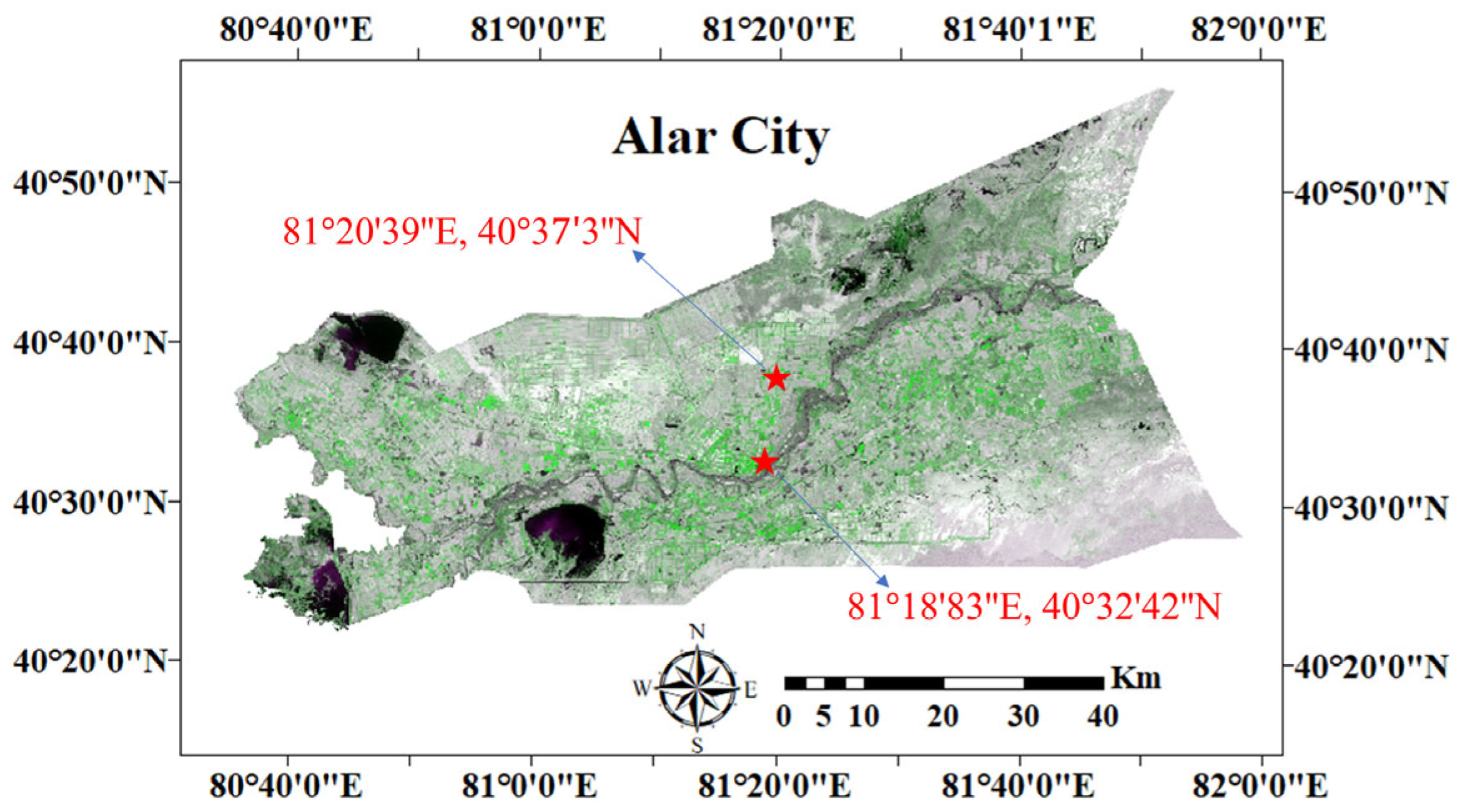
2.1. Experimental Design

Healthy and VW cotton leaves were collected on 30 August 2022 (cotton boll stage) from the Tarim University Agricultural Teaching and Research Practice Base, Alar City, Xinjiang (81°18′83″ E, 40°32′42″ N) and the experimental field with perennial outbreak of VW at Shi Tuan, Alar City, Xinjiang (81°20′39″ E, 40°37′3″ N). The location of the experimental field is shown in Figure 1. The cotton variety selected for the experiment was Tahe 2, which exhibits steady growth throughout the growing period, has medium-sized, dark-green leaves, and is VW tolerant [27].
Four representative collection points were selected within the health cotton trial zone to capture the growth characteristics of cotton plants in the area. Five cotton plants were sampled at each collection point using a five-point sampling method, with leaves excised from the upper, middle, and lower positions of each plant, resulting in a total of 120 healthy leaf samples. The collected cotton leaves were free from any obvious diseases, and included both old and young leaves. To obtain cotton leaves with different severity levels of VW, the disease severity of the leaf was divided into five levels based on the percentage of the diseased area compared to the total leaf area (normal: 0; mild: 0–25%; moderate: 25–50%; severe: 50–75%; extremely severe: 75–100%) [28]. Four collection points were selected within the VW experimental area, where the disease outbreak was concentrated. Six cotton leaves with different disease severity levels and positions were collected from each collection point, resulting in a total of 120 diseased leaf samples. This data collection method plays an important role in expressing the different onset periods of cotton VW. The collected samples were tested on-site for SPAD values and hyperspectral data to ensure the accuracy and validity of the experimental data.

2.2. Hyperspectral Data Acquisition

The ASD FieldSpec HandHeld 2 portable hyperspectral radiometer (325–1075 nm; Analytical Spectral Device, Boulder, CO, USA), with a spectral resolution of 3 nm, was selected for the acquisition of cotton leaf hyperspectral data. Spectral data were acquired between 12:00 and 14:00 local time, and clear and cloudless weather was ensured throughout the acquisition process. A hyperspectral spectrometer requires whiteboard calibration before data acquisition, and calibration should be performed every 15 min. The calibration should ensure that spectral reflectance within the wavelength range is 1 [29,30]. During the collection process, the leaf samples were placed on a black background, and the instrument probe was oriented vertically downward, maintaining a distance of 15–20 cm from the sample at all times. The field of view of the spectrometer was 25°. When measuring the spectra, the experimenter wore dark clothing and faced the direction of sunlight to avoid any influence from shadows or reflections that could affect the spectral properties of the leaves. The experimenter also avoided measuring the properties of the leaf veins. Five spectral curves were collected for each leaf sample, and the average value was considered as the final reflectance information of that sample.

2.3. Determination of SPAD Values

The SPAD-502 portable chlorophyll meter (Konica Minolta, Chiyoda City, Japan) was used for the determination of the SPAD values of cotton leaves. After collecting the spectral data of the leaf samples, the SPAD values were measured at five different locations of the leaves between the leaf margin and the main vein of the lobes, and the average value was considered the final SPAD value of the leaf sample. The main veins are mainly tissues that transport water and nutrients, while the petiole is the part that connects the leaf blade to the stem, and their tissue structure and chemical compositions are different from those of the leaf blade, which may affect the accuracy of the SPAD values of the leaf blade. Therefore, care was taken to avoid the main veins and petioles when measuring.

2.4. Data Processing

2.4.1. Dataset Partitioning

The Mahalanobis distance method was used to eliminate outliers in the spectra and SPAD values [31] and avoid the influence of abnormal data resulting from instrumental or human factors on the final modeling result. To ensure the one-to-one correspondence between spectra and SPAD values, the SPAD values corresponding to anomalous spectra and the spectra corresponding to anomalous SPAD values were synchronized and eliminated. The SPAD values (112 for healthy and 111 for VW cotton leaves) obtained after eliminating abnormal data were sorted from highest to lowest, and every four SPAD values were divided into one group using a stratified sampling method to obtain 28 groups. Each group was then divided into modeling and validation sets in the ratio of 3:1. Finally, 84 modeling and 28 validation samples were obtained for healthy cotton leaves, and 83 modeling and 28 validation samples were obtained for VW cotton leaves.

2.4.2. Spectral Data Preprocessing

The acquisition of spectral data can be easily affected by various factors such as stray light, instrument noise, and baseline drift. Therefore, spectral preprocessing is an important step to mitigate the influence of these unfavorable factors on the obtained sample spectral curve [32,33]. To eliminate random noise in the spectral signal and improve the signal-to-noise ratio in this study, spectral preprocessing was performed based on Savitzky–Golay (SG) smoothing. Mean centering (MC) is one of the most common methods of scaling, which can effectively eliminate the errors resulting from excessive differences in data scales; a standard normal variate (SNV) can eliminate spectral errors caused by factors such as variations in particle size and optical path length, thereby making spectra of samples with similar properties more consistent; multiplicative scatter correction (MSC) is used to eliminate the spectral influence caused by uneven scattering due to particles; reciprocal second-order differentiation ([1/SG]″) and logarithmic second-order differentiation ([lg(SG)]″) can subtract the influence of instrument background or drift on the signal, thereby improving spectral resolution [34,35].

2.4.3. Selection of Spectral Characteristic Bands

The existence of multiple correlations between spectral bands leads to high redundancy in spectral information, which increases the difficulty in modeling at a later stage. Extracting spectral characteristic bands thus becomes an effective way to sieve and reduce data and improve modeling efficiency. In this study, under the premise of spectral preprocessing, correlation coefficients, vegetation indices with clear physical interpretations (Table 1), SPA, and CARS were used to extract spectral characteristic information. In addition, obtaining four vegetation indices with relatively clear physical interpretations under different preprocessing methods is used to explore the sensitivity of selected traditional vegetation indices to spectral preprocessing.
The correlation coefficient was obtained using Pearson’s correlation analysis of the spectral reflectance of each band in the dataset with its corresponding physicochemical parameters to screen for the characteristic bands with the maximum correlation. SPA is a forward iterative selection method that utilizes vector projection analysis to choose the most effective wavelengths with minimal redundancy, thereby addressing collinearity issues [40]. CARS employs an adaptive reweighted sampling technique in each iteration, selecting wavelength points with large absolute regression coefficients in the partial least squares model as a new subset. Based on this new subset, a PLS model is constructed, and through multiple calculations, the subset with the lowest RMSE of cross-validation is selected as the spectral characteristic wavelength [41].

2.5. Model Construction Method

2.5.1. PSO–BP Model

The BP neural network is a multilayer feedforward neural network with input, hidden, and output layers. It uses the BP of the error method to continuously adjust the weights and thresholds between layers to determine network parameters corresponding to the minimum error. However, inappropriate initial weights can result in slow convergence and a tendency to become stuck in local optima during the training process. Therefore, in this study, PSO was used to optimize the weights and thresholds of the BP neural network to reduce the time cost and improve the model estimation accuracy by using its global optimization-seeking capability [42].
PSO is used to design a type of particle that is devoid of volume and mass. Each particle explores the problem space for optimal solutions using randomly generated initial positions and flight directions, considering the identified optimum as its extremum. By sharing these individual extrema, the particle swarm collectively seeks a global optimum solution, thereby adjusting its velocity and position to achieve optimal outcomes [43]. Assuming the existence of a particle swarm consisting of m particles in an N-dimensional space, where the position of the i-th particle is denoted as X i = x i 1 , x i 2 , , x i N , and its velocity as V i = v i 1 , v i 2 , , v i N , the particle’s optimal position is determined by evaluating the objective function as P i = p i 1 , p i 2 , , p i N . The global optimal position of the particle swarm is represented as P g = p g 1 , p g 2 , , p g N . During each iteration, the velocities and positions of the particles are continuously updated based on Equations (1) and (2) [44].
v i n + 1 = ω v i n + c 1 r 1 p i n x i n + c 2 r 2 p g n x i n
x i n + 1 = x i n + v i n + 1
In Formulas (1) and (2), i = 1 ,   2 , ,   m ; n = 1 ,   2 , ,   N ; ω is the inertia weight, which is used to adjust global and local search ability; c 1 and c 2 are the learning factors, which regulate the maximum step of particles flying in the direction of individual and population optima, respectively, and their values are usually in the range of [0, 4]; r 1 and r 2 are random numbers varying in the interval of [0, 1], which are used to maintain the diversity of the particle population.

2.5.2. GWO–ELM Model

ELM is an improved machine learning model based on single hidden-layer feedforward neural network [45]. ELM differs from the traditional neural network based on gradient algorithm BP error to adjust the weights, whose input-layer weights and implicit layer thresholds are generated by random setting. Moreover, the connection weights of the implicit and output layers are calculated using generalized inverse matrix theory, which has the advantages of strong generalization performance and fast learning speed. To avoid the ELM from falling into the local optimum and affecting model estimation accuracy, GWO was used to optimize the ELM in this study.
By simulating the strict hierarchy and hunting mechanism of gray wolf society, GWO labels the three wolves with optimal fitness in the pack as α, β, and δ (in that order), which correspond to the optimal, suboptimal, and third-optimal solutions of the objective optimization function, respectively; and the remaining solutions are labeled as ω. Then, the whole optimization search process of GWO mainly includes encirclement, hunting, and attack [46,47].
The mathematical modeling of the encirclement behavior is as follows:
D = C X p t X t X t + 1 = X p t A D A = 2 a r 1 a C = 2 r 2
In Formula (3), D denotes the distance between the gray wolf and the prey; C and A denote the coefficient vectors; X p and X denote the position vectors of the prey and the gray wolf, respectively; t and a denote the number of current iterations and the convergence factor, respectively; r 1 and r 2 are randomly generated vectors in the interval [0, 1].
The mathematical modeling of the hunting behavior is as follows:
D α = C 1 X α t X t D β = C 2 X β t X t D δ = C 3 X δ t X t
X 1 = X α t A 1 D α X 2 = X β t A 2 D β X 3 = X δ t A 3 D δ
X t + 1 = X 1 + X 2 + X 3 3
In Formula (4), D α , D β , and D δ represent the distances from α, β, and δ, respectively, to ω after t iterations. X α t , X β t , X δ t , and X t denote the current position vectors of α, β, δ, and ω, respectively. C 1 , C 2 , and C 3 represent random disturbances to α, β, and δ wolves, respectively. In Formula (5), X 1 , X 2 , and X 3 represent the step size and direction of ω toward α, β, and δ, respectively. A 1 , A 2 , and A 3 are random vectors. In Formula (6), X t + 1 represents the final position of ω.
The attack behavior is completed by decreasing the convergence factor a in Formula (3). When A is in the interval [−1, 1], the next position of the gray wolf is between the current position and the prey, and the attack behavior is realized by this form; otherwise, the search for the prey continues.

2.5.3. Model Construction Process

To estimate the SPAD value of cotton leaves more accurately, the spectral reflectance data in the wavelength range of 350–1050 nm were selected for the study, and the specific SPAD value estimation model construction process is shown in Figure 2. First, we used a portable hyperspectral radiometer and a portable chlorophyll meter SPAD-502 to acquire the spectral data and SPAD values of the experimental samples, respectively. Second, different preprocessing operations were performed on the original spectral data, and based on the different preprocessing, univariate and multivariate modeling parameters were selected using the characteristic band extraction method. Finally, single and multifactor models were constructed using the characteristic parameters to screen the optimal SPAD estimation model.

2.6. Model Evaluation Statistics

To fully evaluate model performance, the coefficient of determination (R2), RMSE, and mean relative error (MRE) were used as evaluation metrics of the model. The closer R2 converges to 1, the stronger the model is in explaining the dependent variable; the smaller the RMSE and MRE, the higher the accuracy and estimation capability of the model [20]. The calculation formulas for each evaluation metric are as follows, where n is the sample size, y i is the actual value, y ^ i is the predicted value, and y ¯ i is the mean value.
R 2 = i = 1 n y ^ i y ¯ i 2 / i = 1 n y i y ¯ i 2
R M S E = 1 n i = 1 n y ^ i y i 2
M R E = 1 n i = 1 n y ^ i y i y i × 100 %

3. Results

3.1. Statistics of SPAD Values of Cotton Leaves

The statistical characteristics of SPAD values of healthy and VW cotton leaves are shown in Figure 3. The descriptive statistics of SPAD values for each dataset of VW cotton leaves were lower than those for each dataset of healthy cotton leaves, except for the coefficient of variation. The mean SPAD values of the overall datasets of healthy and VW cotton leaves were 64.243 and 59.862, respectively, which were between the mean values of the respective modeling and validation sets. Moreover, the coefficients of variation for each dataset were <10%, which was in accordance with the statistical properties and laid the foundation for the construction of a hyperspectral estimation model for cotton SPAD values under VW stress.

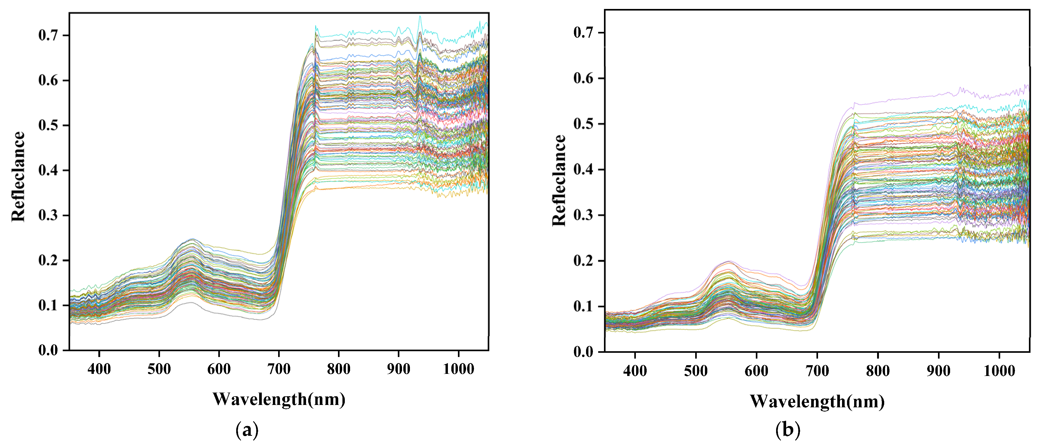
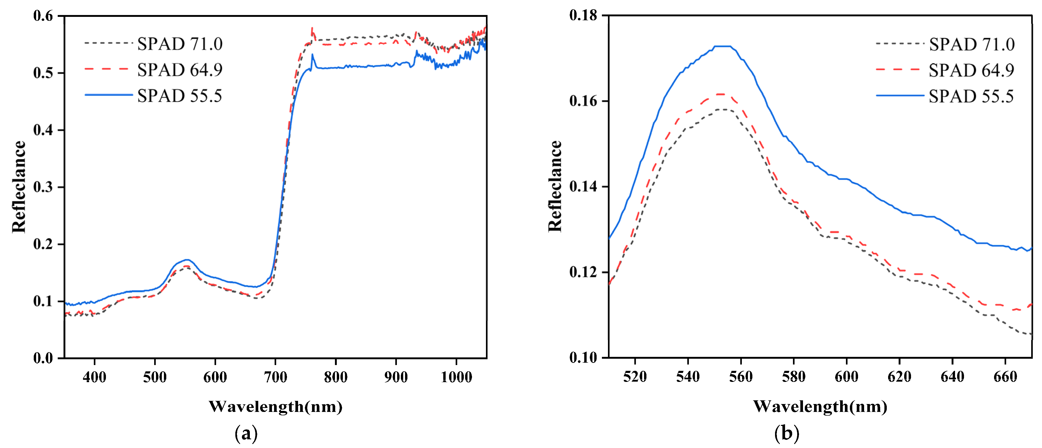
3.2. Spectral Characteristics of Cotton Leaves with Different SPAD Values

The original spectral reflectance curves of healthy and VW cotton leaves are shown in Figure 4a,b, respectively. The spectral reflectance of healthy and VW cotton leaves in the near-infrared wavelength range (780–1050 nm) was between 0.33 and 0.75 and between 0.22 and 0.59, respectively. On average, the spectral reflectance of healthy cotton leaves was higher than that of the leaves affected by VW in this wavelength range. The variation of spectral reflectance with wavelengths for both healthy and VW cotton leaves showed notable characteristics of lower reflectance in the visible band (400–780 nm) and higher reflectance in the near-infrared band (780–1050 nm), and the trends of spectral curves were the same. Due to the absorption of red and blue light by chlorophyll for photosynthesis, both blue and red absorption valleys were formed near the visible-light wavelengths of 490 nm and 670 nm, respectively. Around 550 nm, the green wavelengths resulted in strong reflection, thus forming a weak reflection peak. In addition, the fence structure of leaves caused a sharp increase in reflectance at 690–750 nm and a significant “red edge” phenomenon; due to multiple reflections and refractions of light in the leaf cells, the spectral reflectance formed a high reflectance plateau at 770–900 nm.
In this study, the hyperspectral data of three representative cotton leaves were selected to plot the hyperspectral curves of cotton leaves with different SPAD values. As shown in Figure 5a, the spectral reflectance increased with increasing SPAD values in the near-infrared band from 770 nm to 900 nm. Figure 5b demonstrates that in the visible range, the band with a clear correlation between spectral reflectance and SPAD value was concentrated at 520–670 nm, where the spectral reflectance decreased with increasing SPAD values and vice versa.

3.3. Characteristic Band Selection of Hyperspectral Data

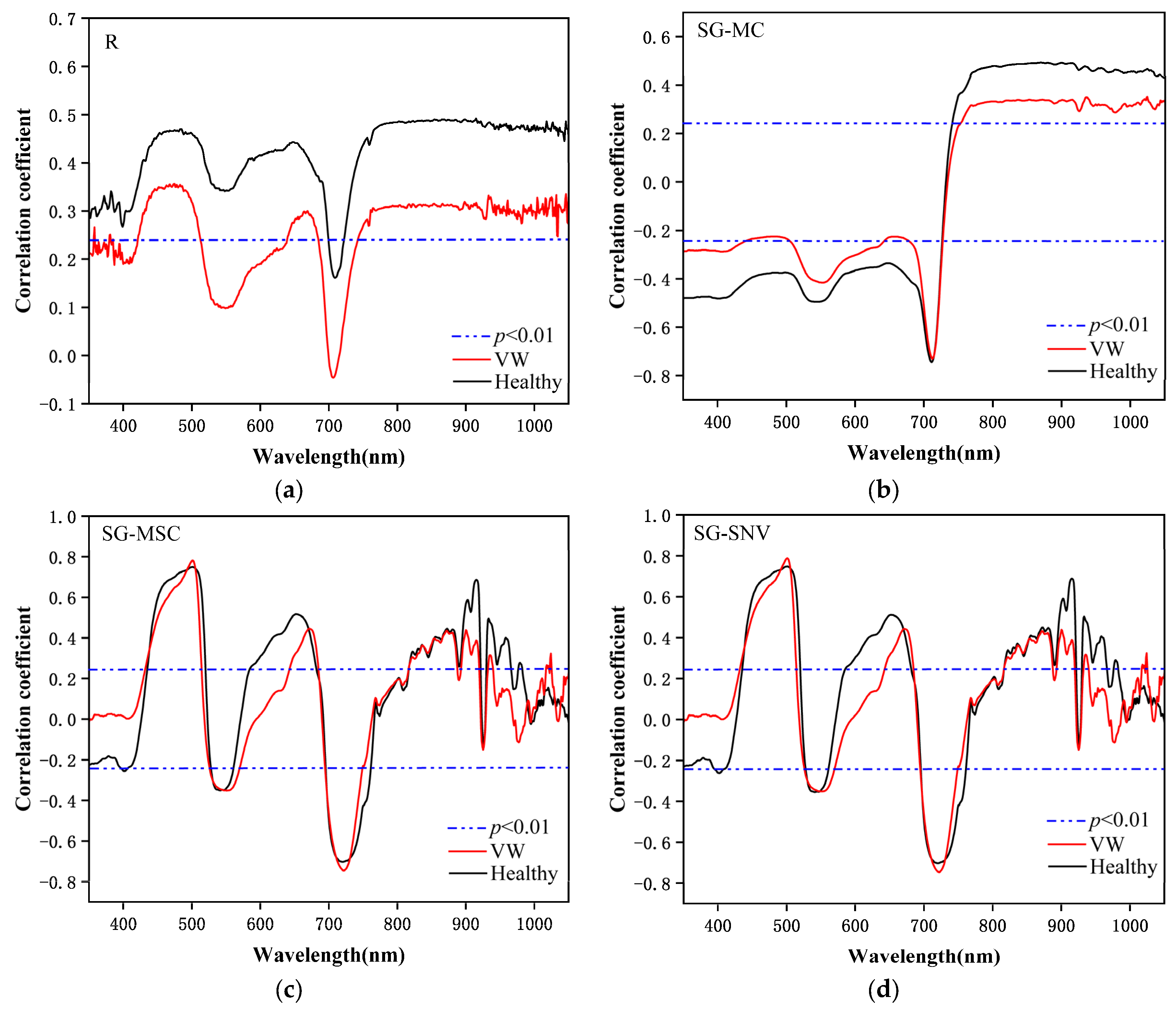
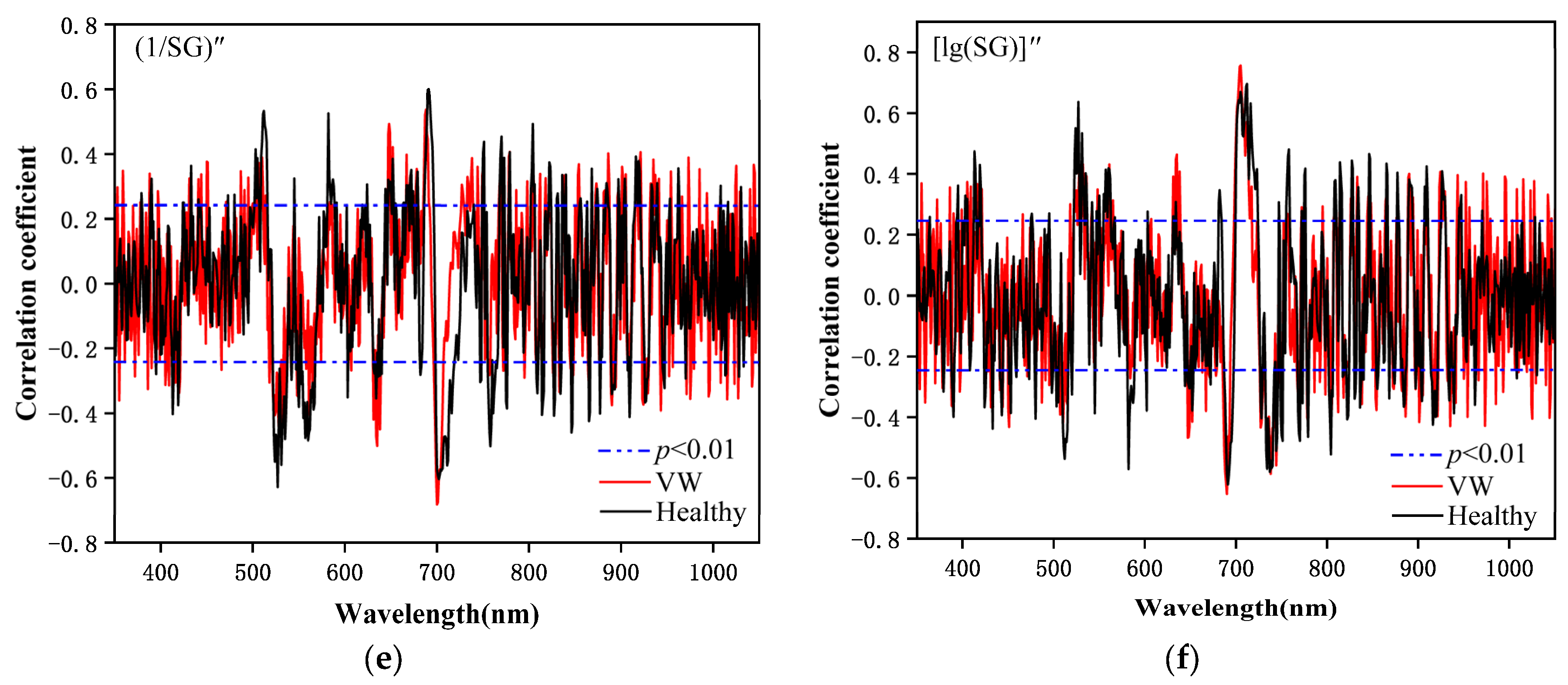
3.3.1. Characteristic Bands Are Selected Based on Correlation Coefficients

The spectral reflectance of each band under different pretreatments was subjected to Pearson’s correlation analysis with the SPAD values of cotton leaves. As shown in Figure 6a–d, the trends of the correlation curves between the spectral reflectance of healthy and VW cotton leaves at each band under the original spectrum (R) and SG-MC, SG-MSC, and SG-SNV pretreatments and the leaf SPAD values were the same, in which the spectral reflectance of VW cotton leaves at 501 nm under SG-SNV pretreatment exhibited the strongest correlation with SPAD value, with the correlation coefficient being 0.788. As shown in Figure 6e,f, the correlation curves between the spectral reflectance and SPAD values in each band after pretreatment with (1/SG)″ and [lg(SG)]″ varied greatly, wherein the spectral reflectance of VW cotton leaves at 705 nm was most strongly correlated with SPAD values under [lg(SG)]″ pretreatment, with the correlation coefficient being 0.757. The original spectral reflectance of healthy and VW cotton leaves was affected by factors, such as stray light and baseline drift, resulting in correlation coefficients between the spectral reflectance in various bands and SPAD values with absolute values below 0.5. However, after preprocessing, the spectral reflectance showed a significant increase in correlation coefficients with SPAD values compared to the original spectral reflectance. Furthermore, after preprocessing, the number of characteristic bands that reached a significant correlation level of 0.01 was higher in healthy cotton leaves compared to VW cotton leaves. In summary, the band with the highest absolute value of the correlation coefficient in each of the five pretreatments was selected as the modeling parameter for the single-factor model to facilitate its construction.

3.3.2. Selection of Characteristic Parameters Based on Vegetation Indices

Based on the four vegetation indices with relatively clear physical descriptions (Table 1), the correlation coefficients between the vegetation indices obtained from healthy and VW cotton leaves under different spectral preprocessing methods and SPAD values were calculated. As shown in Figure 7a,b, the correlation between vegetation indices and SPAD values under different pretreatments was notably different, among which the correlation between the four vegetation indices obtained for (1/SG)″ and [lg(SG)]″ pretreatments and SPAD values was generally low. The correlations of MTCI and mNDVI with SPAD values obtained under the original spectra and SG-MC, SG-MSC, and SG-SNV pretreatments were more stable, with the correlation coefficients stabilizing around 0.68–0.69 and 0.54–0.58, respectively. In addition, the absolute values of the correlation coefficients between TCARI and MCARI obtained under SG-MSC and SG-SNV pretreatments for healthy and VW cotton leaves and SPAD values were >0.6, which was better than the correlation between the vegetation index of original spectra and SPAD values. These results showed that pretreatment by SG-MSC and SG-SNV improved the correlation of TCARI and MCARI with SPAD values.

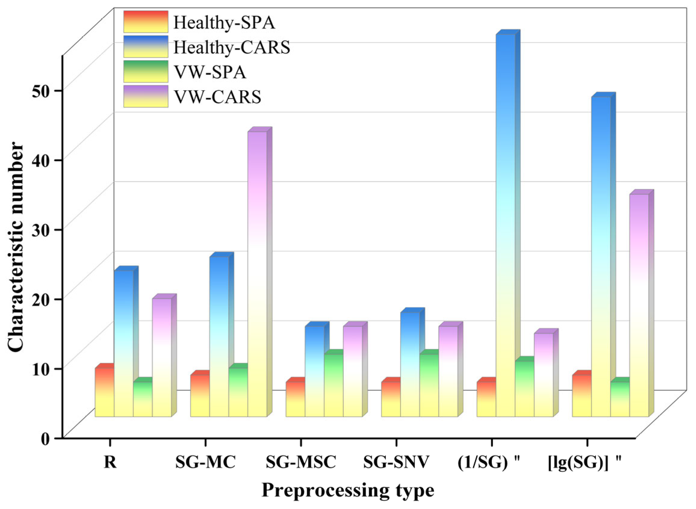
3.3.3. Selection of Characteristic Parameters Based on SPA and CARS

The spectral reflectance of cotton leaves in the range of 350–1050 nm was used as the input quantity for SPA and CARS, and the SPAD value was used as the output quantity. The characteristic variables selected by SPA were controlled between 5 and 30, the number of iterations of CARS was set to 100, and the spectral characteristic bands were selected based on the principle of minimum RMSE. As shown in Figure 8, both SPA and CARS significantly reduced the dimensionality of spectral data, with dimensionality reduction ratios exceeding 92%. The number of spectral feature bands selected by SPA for each preprocessing type ranged from five to nine, with dimensionality reduction ratios exceeding 98%. The dimensionality reduction ratios for the feature bands selected by CARS were above 92%. Among them, the maximum number of feature bands (55) was selected after applying the (1/SG)″ treatment to the spectral reflectance of healthy cotton leaves. In contrast, the minimum number of feature bands (12) was selected after applying the (1/SG)″ treatment to the spectral reflectance of cotton leaves affected by VW.

3.4. Construction and Optimal Selection of Cotton Leaf SPAD Estimation Model

3.4.1. Single-Factor Model Construction

The characteristic bands and vegetation indices with the highest correlation with the SPAD values of cotton leaves under different pretreatments were used as modeling parameters for five single-factor models, which were constructed and screened for the optimal SPAD-value hyperspectral estimation model.
From Table 2, it can be noted that the characteristic band model outperformed the vegetation index model under the same pretreatment type. For healthy cotton leaves, the exponential regression model constructed with spectral reflectance at 711 nm under SG-MC pretreatment as the independent variable was the optimal single-factor model, with the modeling and validation set R2 of 0.558 and 0.642, respectively. For VW cotton leaves, the exponential regression model constructed with spectral reflectance at 501 nm under SG-MSC pretreatment as the independent variable was the optimal single-factor model, with the modeling and validation set R2 of 0.606 and 0.684, respectively. Upon comprehensive analyses, the optimal single-factor model for VW cotton leaves showed a higher estimation accuracy compared to the optimal single-factor model for healthy cotton leaves. However, all single-factor models performed at a relatively low level in terms of the three evaluation indicators, suggesting a mediocre estimation effect.

3.4.2. Multifactor Model Construction Based on PSO–BP

The characteristic bands under different preprocessing methods extracted by SPA and CARS were used as modeling parameters for the PSO–BP model. The number of the BP neural network training time was set to 2000, the target error was 1.00 × 10⁻⁵, the learning rate was 0.1, and the number of nodes in the hidden layer was calculated and adjusted according to the empirical formula. We set the PSO learning factors C1 and C2 to 1.494, with velocity and position ranges of −1 and 1 and −5 and 5, respectively, and applied a trial-and-error approach multiple times to determine the number of hidden layers, population size, and maximum number of iterations. The specific parameter settings are shown in Figure 9.
There were significant differences in the parameter settings of the PSO–BP model based on healthy and VW cotton leaves under different spectral preprocessing methods. The number of nodes in the hidden layers of the model based on healthy and VW cotton leaves was between three and eight, the population size between 10 and 40, and the maximum number of iterations between 50 and 90, where too many nodes in the implicit layer increased the complexity of the network and resulted in overfitting of the model, and too few resulted in underfitting of the model. An extremely large population size could lead to a reduction in the PSO-seeking efficiency, and an extremely small population size could easily fall into a local optimum. Therefore, reasonable adjustment of the parameters of the PSO–BP model according to the actual data was beneficial to improve the overall performance of the model.
The PSO–BP model constructed using different preprocessing and characteristic extraction methods exhibited an estimated effect on the SPAD values of cotton leaves, as shown in Table 3. For healthy cotton leaves, after SG-MC processing, the PSO–BP model constructed using CARS-selected characteristic bands exhibited enhanced estimation of SPAD values, with an R2 of 0.828 and 0.755 and RMSE of 2.038 and 2.433 for the modeling and validation sets, respectively. For VW cotton leaves, after SG-SNV processing, the PSO–BP model constructed using CARS-selected characteristic bands exhibited improved estimation of SPAD values, with an R2 of 0.821 and 0.806 and RMSE of 2.379 and 2.557 for the modeling and validation sets, respectively. Under the same preprocessing method, the estimation accuracy of the model constructed using CARS-extracted characteristic bands was higher than that of SPA, and the estimation effect of the PSO–BP model was better than that of the single-factor model under each preprocessing type. Furthermore, the preprocessed PSO–BP model did not necessarily exhibit higher accuracy in estimating the SPAD values of cotton leaves compared to the PSO–BP model constructed using the original spectra.

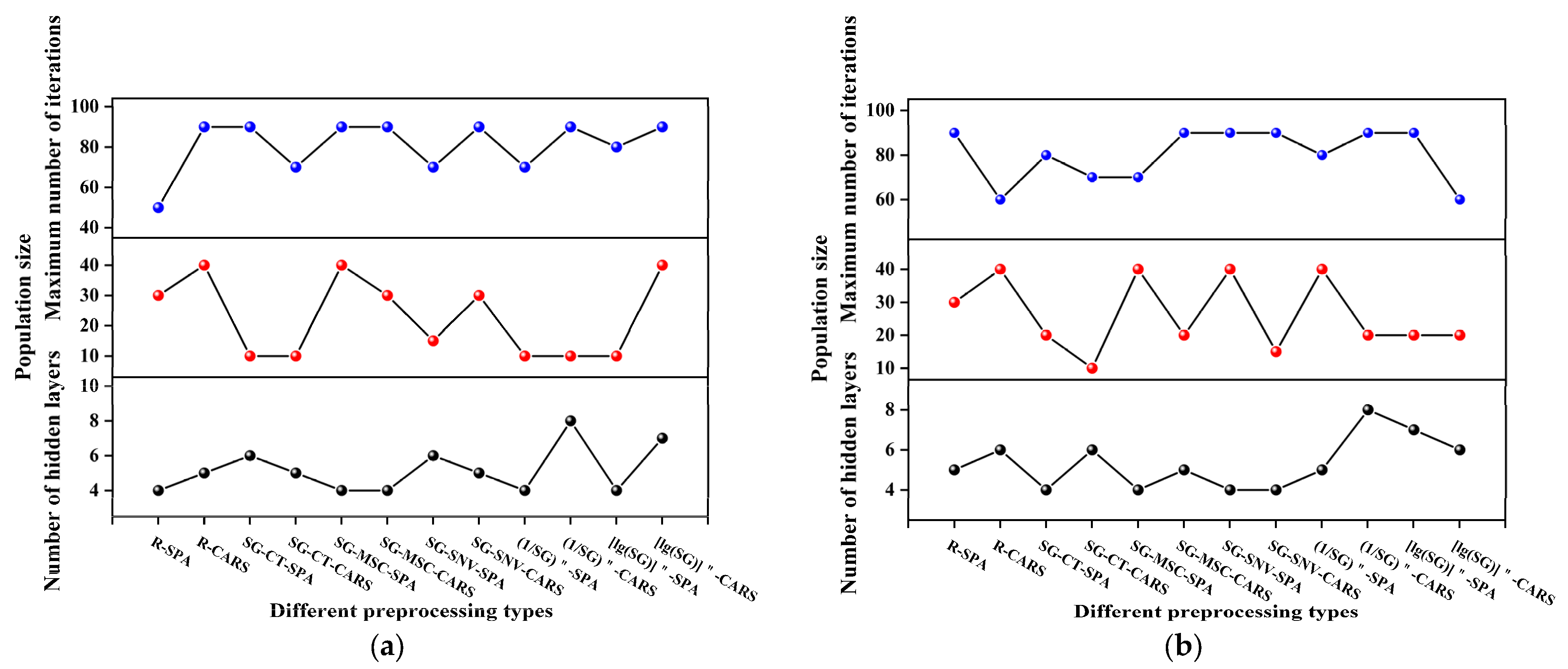
3.4.3. Multifactor Model Construction Based on GWO–ELM

The characteristic bands screened under different preprocessing methods were used as the modeling parameters for GWO–ELM. The smooth and stable sigmoid function, which was easy to derive, was selected as the activation function of ELM, and the multiple trial-and-error method was applied to determine the number of nodes in the hidden layers, the size of the gray wolf population and the maximum number of iterations. The final modeling parameters are shown in Figure 10. The number of hidden-layer nodes based on healthy and VW cotton leaf models with different preprocessing methods and characteristic band-extraction methods ranged from four to eight, the gray wolf population size from 10 to 40, and the maximum number of iterations from 50 to 100. Among them, if the value of the maximum number of iterations—an important condition for the algorithm to stop iterating—was extremely small, it would have caused the algorithm to fail to converge to the global optimal solution, and if its value was extremely high, it would have been time consuming and may have resulted in model overfitting. Therefore, it was crucial to determine the most suitable number of iterations according to the actual data to ensure adequate performance and efficiency of the algorithm.
The estimation effects of the GWO–ELM model on the estimation of SPAD values of healthy and VW cotton leaves are shown in Table 4. For healthy cotton leaves, after [lg(SG)]″ processing, the GWO–ELM model constructed using CARS-selected characteristic bands provided the best estimation of SPAD values, with an R2 of 0.956 and 0.887 and RMSE of 1.026 and 1.654 for the modeling validation sets, respectively. For VW cotton leaves, after SG-MSC processing, the GWO–ELM model constructed using CARS-selected characteristic bands was the best estimation of SPAD values, with an R2 of 0.832 and 0.824 and RMSE of 2.310 and 2.431 for the modeling and validation sets, respectively. Upon comprehensive comparison, the GWO–ELM model was better for estimating the SPAD values of healthy cotton leaves than for estimating the SPAD values of VW cotton leaves.

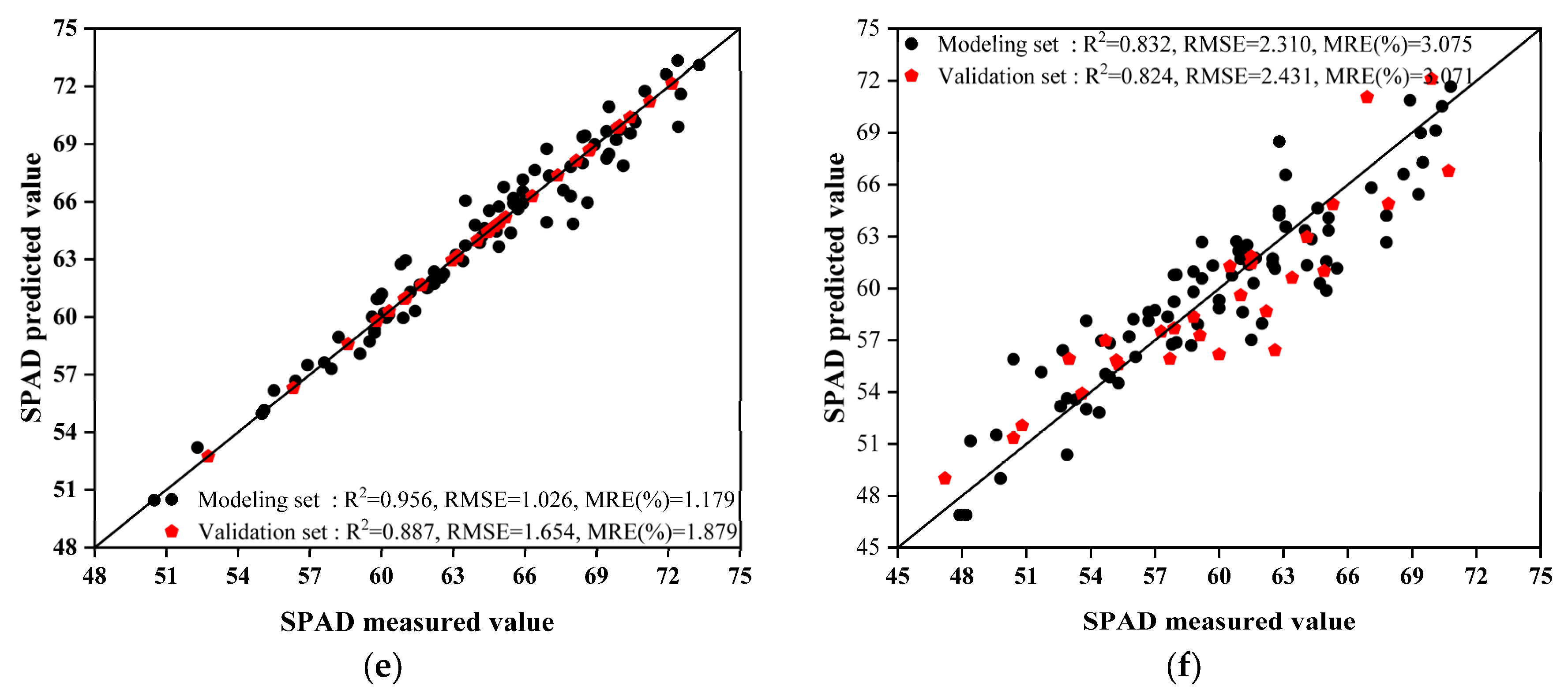
3.4.4. Comparison of Estimation Accuracy among Different Modeling Methods

To comprehensively compare the differences among the three modeling methods, we fitted the measured SPAD values of healthy and VW cotton leaves to the predicted values of the optimal model under each preprocessing method. As shown in Figure 11, the multifactor model exhibited a higher estimation accuracy for the SPAD values of cotton leaves compared to the single-factor model. Additionally, the GWO–ELM model achieved a higher estimation accuracy for the SPAD values of cotton leaves than the PSO–BP model. The accuracy of the single-factor and PSO–BP models in estimating the SPAD values of VW cotton leaves was higher than that for estimating the SPAD values of healthy cotton leaves, whereas the accuracy of the GWO–ELM model in estimating the SPAD values of healthy cotton leaves was higher than that for estimating the SPAD values of VW cotton leaves. Additionally, the [lg(SG)]″–CARS–GWO–ELM model performed the best in estimating the SPAD values of healthy cotton leaves, whereas the SG-MSC–CARS–GWO–ELM model demonstrated the highest accuracy in estimating the SPAD values of cotton leaves affected by VW. Therefore, the GWO–ELM model can be effectively utilized for the estimation of SPAD values of cotton leaves under VW stress.

4. Discussion

Owing to the absorption of visible light energy by chlorophyll, cotton leaves exhibit a low spectral reflectance in the visible light range. However, in the near-infrared range, the cells and cell walls present in the leaves strongly reflect and refract light, resulting in a comparatively higher spectral reflectance of cotton leaves within this range [37]. For healthy cotton leaves, within the visible light range (520–690 nm), the utilization efficiency of light energy increases with the increase in chlorophyll content. Consequently, the spectral reflectance of cotton leaves decreases as chlorophyll content increases within this range. On the other hand, chlorophyll content serves as one of the crucial factors in maintaining the internal stability of cotton leaves. An increase in chlorophyll content indicates a higher level of leaf maturity and increased stability in leaf anatomy. Thus, within the range of 770–900 nm, the spectral reflectance increases with an increase in chlorophyll content, which aligns with the findings of previous studies [13,37,48]. Therefore, estimating the SPAD values of individual cotton leaves using hyperspectral data is feasible.
As the severity of Fusarium wilt increases, the spores and mycelia produced by the pathogen impede water transportation within cotton plants. Furthermore, the toxins produced by the fungal spores disrupt the cellular structure of cotton leaves, resulting in the loss of pigmentation and continuous yellowing of the foliage [49,50]. Furthermore, the spectra of cotton leaves in the near-infrared range are affected because of the effects of pigments and the internal cell structure of leaves. When cotton leaves are infected with VW, the internal tissues and cell structure of the leaves are damaged, resulting in a continuous decrease in chlorophyll content, thereby altering the multiple reflections of light and leading to lower spectral reflectance of VW-infected cotton leaves compared to healthy cotton leaves in the near-infrared range (780–1050 nm). Guo et al. [51] concluded that the internal tissue structure of wheat leaves was damaged by yellow rust infection, resulting in lower spectral reflectance of the infected leaves in the near-infrared range (from 738 nm to 1000 nm) than that of healthy wheat leaves. These results align with the findings of the present study, indicating the feasibility of using hyperspectral techniques to assess the SPAD values of cotton leaves under VW stress. Furthermore, this spectral property can be utilized to estimate the severity of the disease in VW-infected cotton leaves.
Spectral preprocessing can eliminate the interference of stray light, baseline drift, and other factors in the data, and is an important tool to improve modeling results [32]. All five preprocessing methods used in this study enhanced the correlation between the characteristic bands and the SPAD values compared to the original spectra. Among these methods, SG-MSC and SG-SNV preprocessing methods proved to be the most effective. MSC scales and translates the spectrum to render the spectral intensity more uniform across the spectral range, whereas SNV normalizes the mean and variance of the spectrum to a consistent level by subtracting the mean from each wavelength value in the spectrum and dividing it by the standard deviation. These two preprocessing methods improved the consistency of the data while reducing the effect of noise, thus further improving the correlation between the spectral data and the SPAD values. However, the correlation between vegetation indices and SPAD values calculated after employing different preprocessing methods was both enhanced and weakened compared with the original spectra. For healthy cotton leaves, MCARI under SG-SNV variation was the optimal vegetation index; for VW cotton leaves, MTCI obtained using the raw spectra was the optimal vegetation index. The reason for this is that the nature of the preprocessed spectra was changed and it was difficult to fully adapt the traditional vegetation index calculation formula, which was consistent with the results of Guo et al. [52]. Furthermore, the selection of spectral characteristic bands effectively simplified the model and improved its estimation accuracy.
In this study, the SPA and CARS methods were chosen for extracting spectral characteristic bands. The results showed that SPA outperformed CARS in dimensionality reduction, which was consistent with previous studies [53,54]. However, a limited number of characteristic bands may hinder the comprehensive response of the model to SPAD values and potentially affect the estimation effectiveness. In contrast, CARS considers the correlation between different bands and can effectively select characteristic bands that are mutually independent yet exhibit significant predictive power. Therefore, the estimation effectiveness of the model constructed using CARS for characteristic band selection was superior to that of SPA. Moreover, further investigation is needed to explore the combination of CARS and SPA for extracting spectral characteristic bands.
In this study, three modeling methods were used to construct hyperspectral inversion models for SPAD values of healthy and VW cotton leaves. The single-factor model, using a single characteristic as an independent variable, could not completely utilize the abundant information contained in hyperspectral data. As a result, the model failed to fully respond to SPAD values. Therefore, the estimation accuracy of the single-factor model for estimating leaf SPAD values was lower than that of the multifactor model. The BP neural network relies on the setting of initial weights and requires multiple iterations using the BP algorithm to adjust the weights. Its generalization ability and learning rate are lower than ELM. However, both BP neural network and ELM are prone to becoming trapped in local optima [55]. Therefore, in this study, PSO and GWO were introduced to optimize both methods. GWO, due to its strong global search capability, effectively avoided falling into local optima, and the algorithm required fewer parameters and exhibited a faster convergence speed, making it easier to debug [46]. PSO possessed both global search and local optimization abilities and exhibited a wider range of parameters that could be flexibly adjusted, exhibiting a certain level of scalability [44]. In this study, the GWO–ELM model constructed using [lg(SG)]″–CARS processing exhibited better estimation of SPAD values for healthy cotton leaves compared to other models. In contrast, the GWO–ELM model constructed using SG-MSC–CARS processing showed a superior estimation of SPAD values for cotton leaves affected by VW compared to other models. Moreover, the optimal models for both healthy and VW-affected cotton leaves achieved modeling and validation set R2 values >0.82. These results indicated that by extracting characteristic bands through spectral preprocessing and constructing machine learning models based on population optimization algorithms, it is possible to accurately estimate the SPAD values of cotton leaves under VW stress. Therefore, it is feasible to utilize this method for estimating SPAD values of cotton leaves under VW stress. For different crops and diseases, the estimation of leaf SPAD value should be based on the actual data combined with different preprocessing and feature extraction algorithms, and the parameters of the machine learning model based on the population optimization algorithm should be flexibly adjusted to select a more suitable estimation model.

5. Conclusions

The findings of this study revealed that there are significant differences in the correlation between spectral reflectance, vegetation indices, and cotton SPAD values under different preprocessing methods. For healthy cotton leaves, the spectral reflectance at 501 nm exhibited the highest correlation coefficient (0.75) with SPAD values under the SG-MSC method. The MCARI was identified as the optimal vegetation index under the SG-SNV method, with an absolute correlation coefficient of 0.71. For cotton leaves affected by VW, the spectral reflectance at 501 nm exhibited the highest correlation coefficient (0.788) with SPAD values under the SG-SNV method. The MTCI obtained from the original spectral data was identified as the optimal vegetation index, with a correlation coefficient of 0.69. Based on comprehensive analysis, the multifactor model outperformed the single-factor model in terms of estimation of SPAD values. Among them, the GWO–ELM model was identified as the optimal model in this study. The modeling and validation sets of the optimal GWO–ELM model for healthy and VW cotton leaves achieved R2 values >0.82. This model effectively estimated the SPAD values of both healthy and VW cotton leaves. Therefore, this model can be utilized for monitoring cotton growth and leaf SPAD values under VW stress. This study used hyperspectral technology to estimate the SPAD values of healthy and VW cotton leaves in the Alar region of Xinjiang and provides a non-destructive diagnostic method for assessing the nutrition status of cotton leaves under VW stress in this region. Additionally, this approach offers theoretical support for precision management of cotton plants.

Author Contributions

Conceptualization, X.Y. and X.Z.; methodology, X.Y., N.Z. and R.M.; software, X.Y., W.S. and H.B.; validation, X.Z. and N.Z.; formal analysis, X.Y. and D.H.; investigation, N.Z.; resources, X.Z. and N.Z.; data curation, X.Y. and R.M.; writing-original draft preparation, X.Y.; writing-review and editing, X.Y., N.Z. and X.Z.; visualization, X.Y. and D.H.; supervision, N.Z. and X.Z.; project administration, N.Z.; funding acquisition, N.Z. All authors have read and agreed to the published version of the manuscript.

Funding

This work was funded by the National Natural Science Foundation of China, grant numbers 32101621, 62061041, 31960503, and the Bingtuan Science and Technology Program, grant numbers 2022CB001-05, 2021BB023-02, and Tarim University President’s Fund, grant number TDZKSS202345, and Graduate Scientific Research Innovation project of Tarim University, grant number TDGRI202256.

Institutional Review Board Statement

Not applicable.

Data Availability Statement

The data that support the findings of this study are available on request from the corresponding author.

Conflicts of Interest

The authors declare no conflict of interest.

References

  1. Fei, H.; Fan, Z.; Wang, C.; Zhang, N.; Wang, T.; Chen, R.; Bai, T. Cotton Classification Method at the County Scale Based on Multi-Features and Random Forest Feature Selection Algorithm and Classifier. Remote Sens. 2022, 14, 829. [Google Scholar] [CrossRef]
  2. Wu, Y.; Zhang, L.; Zhou, J.; Zhang, X.; Feng, Z.; Wei, F.; Zhao, L.; Zhang, Y.; Feng, H.; Zhu, H. Calcium-Dependent Protein Kinase GhCDPK28 Was Dentified and Involved in Verticillium Wilt Resistance in Cotton. Front. Plant Sci. 2021, 12, 772649. [Google Scholar] [CrossRef] [PubMed]
  3. Fradin, E.F.; Thomma, B.P. Physiology and molecular aspects of Verticillium wilt diseases caused by V. dahliae and V. albo-atrum. Mol. Plant Pathol. 2006, 7, 71–86. [Google Scholar] [CrossRef] [PubMed]
  4. Klosterman, S.J.; Atallah, Z.K.; Vallad, G.E.; Subbarao, K.V. Diversity, pathogenicity, and management of Verticillium species. Annu. Rev. Phytopathol. 2009, 47, 39–62. [Google Scholar] [CrossRef]
  5. Song, R.; Li, J.; Xie, C.; Jian, W.; Yang, X. An Overview of the Molecular Genetics of Plant Resistance to the Verticillium Wilt Pathogen Verticillium dahliae. Int. J. Mol. Sci. 2020, 21, 1120. [Google Scholar] [CrossRef] [PubMed]
  6. Li, Y.; Zhang, X.; Lin, Z.; Zhu, Q.-H.; Li, Y.; Xue, F.; Cheng, S.; Feng, H.; Sun, J.; Liu, F. Comparative transcriptome analysis of interspecific CSSLs reveals candidate genes and pathways involved in Verticillium wilt resistance in cotton (Gossypium hirsutum L.). Ind. Crop. Prod. 2023, 197, 116560. [Google Scholar] [CrossRef]
  7. Ayele, A.G.; Wheeler, T.A.; Dever, J.K. Impacts of Verticillium Wilt on Photosynthesis Rate, Lint Production, and Fiber Quality of Greenhouse-Grown Cotton (Gossypium hirsutum). Plants 2020, 9, 857. [Google Scholar] [CrossRef]
  8. Chen, B.; Li, S.; Wang, K.; Zhou, G.; Bai, J. Evaluating the severity level of cotton Verticillium using spectral signature analysis. Int. J. Remote Sens. 2012, 33, 2706–2724. [Google Scholar] [CrossRef]
  9. Gitelson, A.A.; Gritz, Y.; Merzlyak, M.N. Relationships between leaf chlorophyll content and spectral reflectance and algorithms for non-destructive chlorophyll assessment in higher plant leaves. J. Plant Physiol. 2003, 160, 271–282. [Google Scholar] [CrossRef]
  10. Amirruddin, A.D.; Muharam, F.M.; Ismail, M.H.; Ismail, M.F.; Tan, N.P.; Karam, D.S. Hyperspectral remote sensing for assessment of chlorophyll sufficiency levels in mature oil palm (Elaeis guineensis) based on frond numbers: Analysis of decision tree and random forest. Comput. Electron. Agric. 2020, 169, 105221. [Google Scholar] [CrossRef]
  11. Vesali, F.; Omid, M.; Kaleita, A.; Mobli, H. Development of an android app to estimate chlorophyll content of corn leaves based on contact imaging. Comput. Electron. Agric. 2015, 116, 211–220. [Google Scholar] [CrossRef]
  12. Steele, M.R.; Gitelson, A.A.; Rundquist, D.C. A comparison of two techniques for nondestructive measurement of chlorophyll content in grapevine leaves. Agron. J. 2008, 100, 779–782. [Google Scholar] [CrossRef]
  13. Huang, X.; Guan, H.; Bo, L.; Xu, Z.; Mao, X. Hyperspectral proximal sensing of leaf chlorophyll content of spring maize based on a hybrid of physically based modelling and ensemble stacking. Comput. Electron. Agric. 2023, 208, 107745. [Google Scholar] [CrossRef]
  14. Uddling, J.; Gelang-Alfredsson, J.; Piikki, K.; Pleijel, H. Evaluating the relationship between leaf chlorophyll concentration and SPAD-502 chlorophyll meter readings. Photosynth. Res. 2007, 91, 37–46. [Google Scholar] [CrossRef] [PubMed]
  15. Tan, L.; Zhou, L.; Zhao, N.; He, Y.; Qiu, Z. Development of a low-cost portable device for pixel-wise leaf SPAD estimation and blade-level SPAD distribution visualization using color sensing. Comput. Electron. Agric. 2021, 190, 106487. [Google Scholar] [CrossRef]
  16. Cavallo, D.P.; Cefola, M.; Pace, B.; Logrieco, A.F.; Attolico, G. Contactless and non-destructive chlorophyll content prediction by random forest regression: A case study on fresh-cut rocket leaves. Comput. Electron. Agric. 2017, 140, 303–310. [Google Scholar] [CrossRef]
  17. Shen, L.; Gao, M.; Yan, J.; Wang, Q.; Shen, H. Winter Wheat SPAD Value Inversion Based on Multiple Pretreatment Methods. Remote Sens. 2022, 14, 4660. [Google Scholar] [CrossRef]
  18. Osco, L.P.; Ramos, A.P.M.; Moriya, É.A.S.; Bavaresco, L.G.; Lima, B.C.D.; Estrabis, N.; Pereira, D.R.; Creste, J.E.; Júnior, J.M.; Gonçalves, W.N.; et al. Modeling hyperspectral response of water-stress induced lettuce plants using artificial neural networks. Remote Sens. 2019, 11, 2797. [Google Scholar] [CrossRef]
  19. Sonobe, R.; Yamashita, H.; Mihara, H.; Morita, A.; Ikka, T. Hyperspectral reflectance sensing for quantifying leaf chlorophyll content in wasabi leaves using spectral pre-processing techniques and machine learning algorithms. Int. J. Remote Sens. 2021, 42, 1311–1329. [Google Scholar] [CrossRef]
  20. Zhang, J.; Zhang, D.; Cai, Z.; Wang, L.; Wang, J.; Sun, L.; Fan, X.; Shen, S.; Zhao, J. Spectral technology and multispectral imaging for estimating the photosynthetic pigments and SPAD of the Chinese cabbage based on machine learning. Comput. Electron. Agric. 2022, 195, 106814. [Google Scholar] [CrossRef]
  21. Mao, Z.-H.; Deng, L.; Duan, F.-Z.; Li, X.-J.; Qiao, D.-Y. Angle effects of vegetation indices and the influence on prediction of SPAD values in soybean and maize. Int. J. Appl. Earth Obs. Geoinf. 2020, 93, 102198. [Google Scholar] [CrossRef]
  22. Wang, T.; Gao, M.; Cao, C.; You, J.; Zhang, X.; Shen, L. Winter wheat chlorophyll content retrieval based on machine learning using in situ hyperspectral data. Comput. Electron. Agric. 2022, 193, 106728. [Google Scholar] [CrossRef]
  23. Sudu, B.; Rong, G.; Guga, S.; Li, K.; Zhi, F.; Guo, Y.; Zhang, J.; Bao, Y. Retrieving SPAD values of summer maize using UAV hyperspectral data based on multiple machine learning algorithm. Remote Sens. 2022, 14, 5407. [Google Scholar] [CrossRef]
  24. Lu, J.; Qiu, H.; Zhang, Q.; Lan, Y.; Wang, P.; Wu, Y.; Mo, J.; Chen, W.; Niu, H.; Wu, Z. Inversion of chlorophyll content under the stress of leaf mite for jujube based on model PSO-ELM method. Front. Plant Sci. 2022, 13, 1009630. [Google Scholar] [CrossRef] [PubMed]
  25. Yang, Y.; Nan, R.; Mi, T.; Song, Y.; Shi, F.; Liu, X.; Wang, Y.; Sun, F.; Xi, Y.; Zhang, C. Rapid and Nondestructive Evaluation of Wheat Chlorophyll under Drought Stress Using Hyperspectral Imaging. Int. J. Mol. Sci. 2023, 24, 5825. [Google Scholar] [CrossRef]
  26. Zhang, J.; Tian, H.; Wang, D.; Li, H.; Mouazen, A.M. A novel spectral index for estimation of relative chlorophyll content of sugar beet. Comput. Electron. Agric. 2021, 184, 106088. [Google Scholar] [CrossRef]
  27. Li, Q.; Li, D.; Xu, A.; Liu, H. Breeding and cultivation techniques of a new cotton variety, Tahe 2. China Cotton 2020, 47, 30+41. [Google Scholar] [CrossRef]
  28. Chen, B.; Li, S.-K.; Wang, K.-R.; Wang, F.-Y.; Xiao, C.-H.; Pan, W.-C. Study on hyperspectral estimation of pigment contents in leaves of cotton under disease stress. Spectrosc. Spectr. Anal. 2010, 30, 421–425. [Google Scholar] [CrossRef]
  29. Ren, P.; Feng, M.-C.; Yang, W.-D.; Wang, C.; Liu, T.-T.; Wang, H.-Q. Response of winter wheat (Triticum aestivum L.) hyperspectral characteristics to low temperature stress. Spectrosc. Spectr. Anal. 2014, 34, 2490–2494. [Google Scholar] [CrossRef]
  30. Wang, J.; Song, X.; Mei, X.; Yang, G.; Li, Z.; Li, H.; Meng, Y. Sensitive bands selection and nitrogen content monitoring of rice based on Gaussian regression analysis. Spectrosc. Spectr. Anal. 2021, 41, 1722–1729. [Google Scholar]
  31. Sun, J.; Zhou, X.; Wu, X.; Zhang, X.; Li, Q. Identification of moisture content in tobacco plant leaves using outlier sample eliminating algorithms and hyperspectral data. Biochem. Biophys. Res. Commun. 2016, 471, 226–232. [Google Scholar] [CrossRef] [PubMed]
  32. Yang, W.; Xiong, Y.; Xu, Z.; Li, L.; Du, Y. Piecewise preprocessing of near-infrared spectra for improving prediction ability of a PLS model. Infrared Phys. Technol. 2022, 126, 104359. [Google Scholar] [CrossRef]
  33. Mishra, P.; Biancolillo, A.; Roger, J.M.; Marini, F.; Rutledge, D.N. New data preprocessing trends based on ensemble of multiple preprocessing techniques. Trends Anal. Chem. 2020, 132, 116045. [Google Scholar] [CrossRef]
  34. Miloš, B.; Bensa, A.; Japundžić-Palenkić, B. Evaluation of Vis-NIR preprocessing combined with PLS regression for estimation soil organic carbon, cation exchange capacity and clay from eastern Croatia. Geoderma Reg. 2022, 30, e00558. [Google Scholar] [CrossRef]
  35. Saberioon, M.; Císař, P.; Labbé, L.; Souček, P.; Pelissier, P. Spectral imaging application to discriminate different diets of live rainbow trout (Oncorhynchus mykiss). Comput. Electron. Agric. 2019, 165, 104949. [Google Scholar] [CrossRef]
  36. Haboudane, D.; Miller, J.R.; Tremblay, N.; Zarco-Tejada, P.J.; Dextraze, L. Integrated narrow-band vegetation indices for prediction of crop chlorophyll content for application to precision agriculture. Remote Sens. Environ. 2002, 81, 416–426. [Google Scholar] [CrossRef]
  37. Daughtry, C.S.T.; Walthall, C.L.; Kim, M.S.; Brown de Colstoun, E.; McMurtrey, J.E. Estimating corn leaf chlorophyll concentration from leaf and canopy reflectance. Remote Sens. Environ. 2000, 74, 229–239. [Google Scholar] [CrossRef]
  38. Dash, J.; Curran, P.J. The MERIS terrestrial chlorophyll index. Int. J. Remote Sens. 2004, 25, 5403–5413. [Google Scholar] [CrossRef]
  39. Sims, D.A.; Gamon, J.A. Relationships between leaf pigment content and spectral reflectance across a wide range of species, leaf structures and developmental stages. Remote Sens. Environ. 2002, 81, 337–354. [Google Scholar] [CrossRef]
  40. Araújo, M.C.U.; Saldanha, T.C.B.; Galvao, R.K.H.; Yoneyama, T.; Chame, H.C.; Visani, V. The successive projections algorithm for variable selection in spectroscopic multicomponent analysis. Chemom. Intell. Lab. Syst. 2001, 57, 65–73. [Google Scholar] [CrossRef]
  41. Li, H.; Liang, Y.; Xu, Q.; Cao, D. Key wavelengths screening using competitive adaptive reweighted sampling method for multivariate calibration. Anal. Chim. Acta 2009, 648, 77–84. [Google Scholar] [CrossRef]
  42. Zhang, Y.; Cui, N.; Feng, Y.; Gong, D.; Hu, X. Comparison of BP, PSO-BP and statistical models for predicting daily global solar radiation in arid Northwest China. Comput. Electron. Agric. 2019, 164, 104905. [Google Scholar] [CrossRef]
  43. Kennedy, J.; Eberhart, R. Particle Swarm Optimization. In Proceedings of the ICNN’95-International Conference on Neural Networks, Perth, Australia, 27 November–1 December 1995; pp. 1942–1948. [Google Scholar] [CrossRef]
  44. Deng, Y.; Xiao, H.; Xu, J.; Wang, H. Prediction model of PSO-BP neural network on coliform amount in special food. Saudi J. Biol. Sci. 2019, 26, 1154–1160. [Google Scholar] [CrossRef]
  45. Huang, G.-B.; Zhu, Q.-Y.; Siew, C.-K. Extreme learning machine: A new learning scheme of feedforward neural networks. In Proceedings of the 2004 IEEE International Joint Conference on Neural Networks (IEEE Cat. No. 04CH37541), Budapest, Hungary, 25–29 July 2004; pp. 985–990. [Google Scholar] [CrossRef]
  46. Mirjalili, S.; Mirjalili, S.M.; Lewis, A. Grey wolf optimizer. Adv. Eng. Softw. 2014, 69, 46–61. [Google Scholar] [CrossRef]
  47. Kunhare, N.; Tiwari, R.; Dhar, J. Intrusion detection system using hybrid classifiers with meta-heuristic algorithms for the optimization and feature selection by genetic algorithm. Comput. Electr. Eng. 2022, 103, 108383. [Google Scholar] [CrossRef]
  48. Zhang, N.; Zhang, X.; Shang, P.; Ma, R.; Yuan, X.; Li, L.; Bai, T. Detection of Cotton Verticillium Wilt Disease Severity Based on Hyperspectrum and GWO-SVM. Remote Sens. 2023, 15, 3373. [Google Scholar] [CrossRef]
  49. Yang, M.; Huang, C.; Kang, X.; Qin, S.; Ma, L.; Wang, J.; Zhou, X.; Lv, X.; Zhang, Z. Early Monitoring of Cotton Verticillium Wilt by Leaf Multiple “Symptom” Characteristics. Remote Sens. 2022, 14, 5241. [Google Scholar] [CrossRef]
  50. Jing, X.; Huang, W.-J.; Wang, J.-H.; Wang, J.-D.; Wang, K.-R. Hyperspectral inversion models on verticillium wilt severity of cotton leaf. Spectrosc. Spectr. Anal. 2009, 29, 3348–3352. [Google Scholar] [CrossRef]
  51. Guo, A.; Huang, W.; Ye, H.; Dong, Y.; Ma, H.; Ren, Y.; Ruan, C. Identification of wheat yellow rust using spectral and texture features of hyperspectral images. Remote Sens. 2020, 12, 1419. [Google Scholar] [CrossRef]
  52. Guo, S.; Chang, Q.; Cui, X.; Zhang, Y.; Chen, Q.; Jiang, D.; Luo, L. Hyperspectral estimation of maize SPAD value based on spectrum transformation and SPA-SVR. J. Northeast Agric. Univ. 2021, 52, 79–88. [Google Scholar] [CrossRef]
  53. Xie, C.; Wang, Q.; He, Y. Identification of different varieties of sesame oil using near-infrared hyperspectral imaging and chemometrics algorithms. PLoS ONE 2014, 9, e98522. [Google Scholar] [CrossRef] [PubMed]
  54. Zhu, S.; Chao, M.; Zhang, J.; Xu, X.; Song, P.; Zhang, J.; Huang, Z. Identification of Soybean Seed Varieties Based on Hyperspectral Imaging Technology. Sensors 2019, 19, 5225. [Google Scholar] [CrossRef] [PubMed]
  55. Liu, H.; Zhu, J.; Yin, H.; Yan, Q.; Liu, H.; Guan, S.; Cai, Q.; Sun, J.; Yao, S.; Wei, R. Extreme learning machine and genetic algorithm in quantitative analysis of sulfur hexafluoride by infrared spectroscopy. Appl. Opt. 2022, 61, 2834–2841. [Google Scholar] [CrossRef] [PubMed]
Figure 1. Location of the experimental field.
Agriculture 13 01779 g001
Figure 2. Overall flow of model construction.
Agriculture 13 01779 g002
Figure 3. Statistical characteristics of SPAD values of cotton leaves.
Agriculture 13 01779 g003
Figure 4. Original spectral reflectance curves of cotton leaves. (a) Spectral curves of healthy cotton leaves; (b) spectral curves of VW cotton leaves.
Agriculture 13 01779 g004
Figure 5. Hyperspectral curves of cotton leaves with different SPAD values. (a) Spectral curves from 350 to 1050 nm; (b) spectral curves from 510 to 670 nm.
Agriculture 13 01779 g005
Figure 6. Correlation coefficients between spectral reflectance and SPAD values under different pretreatments. (a) R; (b) SG-MC; (c) SG-MSC; (d) SG-SNV; (e) [1/SG]″; (f) [lg(SG)]″.
Agriculture 13 01779 g006aAgriculture 13 01779 g006b
Figure 7. Correlation between vegetation indices and SPAD values under different pretreatments. (a) Healthy cotton leaves; (b) VW cotton leaves.
Agriculture 13 01779 g007
Figure 8. Selection of multivariate characteristic parameters of different pretreatment types.
Agriculture 13 01779 g008
Figure 9. PSO–BP modeling parameters. (a) Healthy cotton leaves; (b) VW cotton leaves.
Agriculture 13 01779 g009
Figure 10. GWO-ELM modeling parameters. (a) Healthy cotton leaves; (b) VW cotton leaves.
Agriculture 13 01779 g010
Figure 11. Optimal model fitting results under different modeling methods. (a) Optimal single-factor model for healthy cotton leaves; (b) optimal single-factor model for VW cotton leaves; (c) optimal PSO–BP model for healthy cotton leaves; (d) optimal PSO–BP model for VW cotton leaves; (e) optimal GWO–ELM model for healthy cotton leaves; (f) optimal GWO–ELM model for VW cotton leaves.
Agriculture 13 01779 g011aAgriculture 13 01779 g011b
Table 1. Estimation method of vegetation indices.
Vegetation IndexExpressionReference
TCARI (Transformed Chlorophyll Absorption in Reflectance Index) 3 R 700 R 670 0.2 R 700 R 550 R 700 / R 670 [36]
MCARI (Modified Chlorophyll Absorption in Reflectance Index) R 700 R 670 0.2 R 700 R 550 R 700 / R 670 [37]
MTCI (MERIS Terrestrial Chlorophyll Index) R 754 R 709 / R 709 R 681 [38]
mNDVI (modified Normalized Difference Vegetation Index) R 750 R 705 / R 750 + R 705 2 R 445 [39]
Table 2. Optimal single-factor model under different pretreatments.
Leaf TypePreprocessing TypeModeling ParameterRegression EquationModeling SetValidation Set
R2RMSEMRE (%)R2RMSEMRE (%)
HealthyRMTCI y = 59.357 + 11.618 ln ( x 0.679 ) 0.4673.5904.5040.6223.1033.917
SG-MC R 711 y = exp ( 3.984 4.785 x 20.303 x 2 ) 0.5583.2704.2190.6422.9394.052
MTCI y = 58.945 + 11.919 ln ( x 0.648 ) 0.4583.6204.5350.6243.1063.880
SG-MSC R 501 y = 71.571 + 1064.254 x 0.5723.2174.0720.5343.3694.445
TCARI y = 34.992 x 0.318 0.4703.5824.5250.5623.3204.133
SG-SNV R 501 y = 266.037 ln ( x + 2.241 ) 0.5723.2194.0760.5283.3894.492
MCARI y = 97.283 177.281 x 0.4893.5164.4630.5533.3394.108
(1/SG)″ R 527 y = 67.803 1349.549 x 0.4703.5794.5100.1874.5065.917
TCARI y = exp ( 4.183 0.935 x 19.829 x 2 ) 0.2494.2625.3990.2234.3525.680
[lg(SG)]″ R 712 y = 64.139 ( 1 + x ) 260.585 0.4863.5244.4290.4893.5744.594
VWRMTCI y = exp ( 3.935 + 0.042 x + 0.021 x 2 ) 0.4104.3245.9480.6633.4894.767
SG-MC R 712 y = 55.270 228.301 x + 96.747 x 2 0.4724.0905.4410.7063.1533.861
MTCI y = exp ( 3.946 + 0.03 x + 0.023 x 2 ) 0.4044.3475.9980.6623.5214.828
SG-MSC R 501 y = exp ( 4.193 31.607 x + 346.534 x 2 ) 0.6063.5344.6360.6843.4094.505
MTCI y = 52.349 + 0.466 x + 1.766 x 2 0.4034.3486.0010.6653.5074.813
SG-SNV R 501 y = 310.754 + 254.762 x 0.6143.4964.5960.6653.5464.705
MCARI y = 28.428 13.135 ln ( x 0.108 ) 0.4324.2435.8430.6103.6584.776
(1/SG)″ R 700 y = 62.534 429.255 x 16 , 515.037 x 2 0.5033.9675.2980.5393.9585.168
TCARI y = 61.536 69.766 x + 151.064 x 2 0.2914.7396.3370.2734.9986.464
[lg(SG)]″ R 705 y = 63.426 + 12 , 574.159 x 5 , 974 , 669.563 x 2 0.5463.7935.2580.6743.3484.567
Table 3. Results of PSO–BP model based on different pretreatments and characteristic selection methods.
MethodHealthyVW
Modeling SetValidation SetModeling SetValidation Set
R2RMSEMRE (%)R2RMSEMRE (%)R2RMSEMRE (%)R2RMSEMRE (%)
R-SPA0.7882.2652.8550.7152.6223.5400.7182.9894.0010.7372.9723.580
R-CARS0.7892.2612.7860.7492.4603.1410.8022.5053.2990.7672.7973.592
SG-MC-SPA0.7162.6203.3980.6610.8613.9050.7033.0684.2580.7053.1494.059
SG-MC-CARS0.8282.0382.5270.7552.4333.0130.8012.5113.4940.7502.9013.801
SG-MSC-SPA0.7352.5323.1640.7132.6333.5330.7652.7313.7150.7882.6703.428
SG-MSC-CARS0.7512.4533.1260.7342.5343.3770.8172.4113.2940.7952.6253.646
SG-SNV-SPA0.6752.8033.5130.7352.5303.3520.8042.4933.3770.7772.7373.659
SG-SNV-CARS0.7652.3862.9150.7422.4962.8590.8212.3793.1820.8062.5573.395
(1/SG)″-SPA0.5273.3844.5130.4983.4804.4970.6463.3494.4210.6753.3054.109
(1/SG)″-CARS0.7652.3852.7110.5843.1714.0200.7242.9583.9670.7902.6583.623
[lg(SG)]″-SPA0.5753.2084.0740.4213.7384.8640.6243.4504.6940.7113.1184.315
[lg(SG)]″-CARS0.8012.1942.7430.7272.5693.2340.7792.6443.4750.7812.7113.751
Table 4. Results of the GWO–ELM model based on different pretreatments and characteristic selection methods.
MethodHealthyVW
Modeling SetValidation SetModeling SetValidation Set
R2RMSEMRE (%)R2RMSEMRE (%)R2RMSEMRE (%)R2RMSEMRE (%)
R-SPA0.7592.4163.0450.7142.6283.5210.7422.8613.9550.7452.9293.857
R-CARS0.8182.0992.6410.7412.5003.3640.8182.3993.1330.7622.8323.426
SG-MC-SPA0.7512.4563.1470.6852.7583.5600.7692.7033.6970.6823.2714.497
SG-MC-CARS0.7882.2632.9070.7782.3133.1860.8302.3233.1460.8062.5553.057
SG-MSC-SPA0.7052.6733.4300.7662.3763.1730.7922.5693.3430.8012.5873.461
SG-MSC-CARS0.7532.4423.0640.8092.1502.7570.8322.3103.0750.8242.4313.071
SG-SNV-SPA0.7092.6523.3210.7702.3563.1190.8032.4973.3040.8082.5403.263
SG-SNV-CARS0.7612.4033.0630.8232.0662.8050.8162.4153.1970.8002.5923.408
(1/SG)″-SPA0.5453.3194.3960.4913.5064.5000.6733.2174.3340.6843.2604.178
(1/SG)″-CARS0.9101.4751.9760.7422.4973.2750.8082.4673.2850.8172.4783.338
[lg(SG)]″-SPA0.6362.9663.9200.4743.5634.7270.7013.0783.9980.6993.1824.427
[lg(SG)]″-CARS0.9561.0261.1790.8871.6541.8790.8362.2773.0110.7622.8304.167
Disclaimer/Publisher’s Note: The statements, opinions and data contained in all publications are solely those of the individual author(s) and contributor(s) and not of MDPI and/or the editor(s). MDPI and/or the editor(s) disclaim responsibility for any injury to people or property resulting from any ideas, methods, instructions or products referred to in the content.

