Optimization of Shifting Quality for Hydrostatic Power-Split Transmission with Single Standard Planetary Gear Set

Abstract

To improve the driving comfort of continuously variable transmission (CVT) tractors, the shifting quality of hydrostatic power-split transmission with a standard planetary gear set was optimized. Firstly, the powertrain of the CVT and two shift strategies, direct-shift and bridge-shift, were introduced; then, a dynamic model of tractor shifting was constructed, and the models of key components such as wet clutches and proportional pressure valves were experimentally verified. Finally, the control parameters of the above two shifting strategies were optimized, and the acceleration impact and sliding energy loss caused by them were compared. The results showed the following: the minimum peak acceleration of the bridge-shift method was 0.385807 m/s²; the energy consumption of the bridge-shift method was significantly lower than that of the direct-shift method; the sliding friction work of clutches decreased by 14.92% and 75.84%, respectively, while their power loss decreased by 22.82% and 74.48%, respectively.

1. Introduction

The working conditions of tractors are complex, as they require more gears to meet different operational needs, but this also leads to complex transmission structures and difficult gear selection. Tractors with continuously variable transmission (CVT) can effectively solve the above problems. At present, there are three common forms of tractor CVT [1,2,3]: hydrostatic transmission, steel belt transmission, and hydrostatic power-split transmission. Among them, the energy consumption of hydrostatic transmission is very high, and the torque transmitted by steel belt transmission is very limited, while hydrostatic power-split transmission has both a high efficiency and a large load driving capacity [4,5,6]. Since the release of the first CVT tractor “926 Vario” by Fent in 1996, hydrostatic power-split transmissions have gradually been applied to various pieces agricultural machinery [7]. Afterwards, transmission manufacturers began to introduce various concepts of tractor CVTs [8,9], such as the Eccom produced by ZF and the Autopowr produced by John Deere. The above-mentioned transmissions all adopt multi-range technology to achieve continuous speed adjustment [10,11,12], so it is necessary to conduct research to improve the quality of the shift [13,14,15], including changing the gear ratio, the clutch engagement time, and the displacement ratio of the swash plate axial piston units. For tractors with heavy load operations such as plowing as their main operating conditions, while paying attention to their riding comfort we also need to consider issues such as power interruption and clutch damage, all of which are important criteria for evaluating the shifting quality. Typically, cascading multiple planetary gears together to form a compound planetary gear set can improve the shifting quality through speed synchronization [10]. This is currently the mainstream strategy for CVT design, as its shifting logic is very simple. In this research field, Bao et al. [16] constructed a clutch control system based on solenoid directional valves and optimized the clutch pressure, the flow, and the displacement ratio of the pump to the motor to improve the shifting quality of the power-split CVT. Chen et al. [17] proposed a simulation model of a similar hydraulic control system, making it possible to further study the shifting dynamics of CVT tractors through computer simulation. Iqbal et al. [18] conducted similar work. Wang et al. [19] analyzed the reliability of clutch control systems based on on–off logic and discussed the possible influence of hydraulic system failures on the shifting quality. To further improve the shifting quality of this type of transmission, it is necessary to use proportional pressure valves to accurately control the clutch action. For example, Xiang et al. [20] proposed a control strategy for dual-clutch transmissions that can maintain the sliding in the torque phase to improve the shifting quality. Li and Görges [21] conducted similar work. Li et al. [22] used a PID controller to track the pressure of the clutch to ensure the repeatability of proportional pressure control. Although a compound planetary gear set can improve the shifting smoothness through speed synchronization, its structure needs to fully consider support and load balance issues when applied, which brings difficulties to its design, manufacturing, and assembly. In contrast, using a single standard planetary gear to merge the power is simple and cost effective. Currently, some companies such as Hofer have shown great interest in this new concept of transmission. However, the shift logic of the transmission is complex, requiring the simultaneous adjustment of multiple wet clutches and swash plate axial piston units during shifting, which is much more difficult to control than traditional power-split CVTs. To improve the shifting quality of this cost-effective power-split CVT with a single planetary gear set and promote its application in tractors, a new strategy called the bridge-shift method is proposed in this study.

2. Materials and Methods

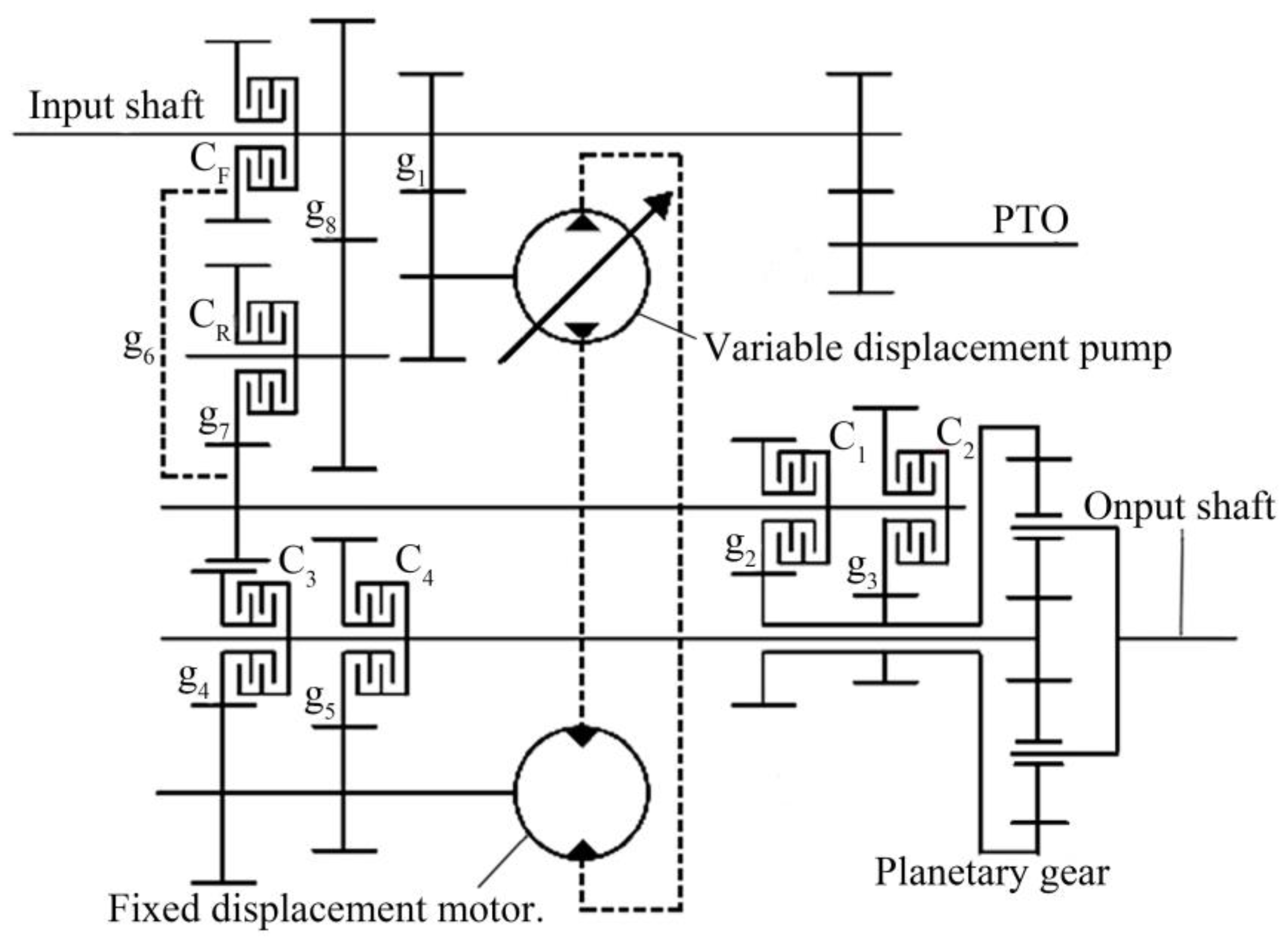
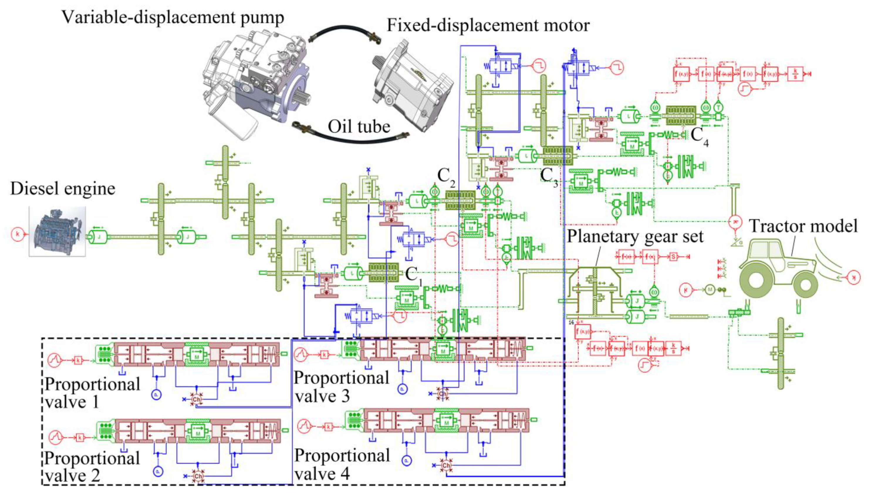
2.1. Powertrain

The hydrostatic power-split transmission proposed in this study has two ranges, HM₁ and HM₂, in the forward direction, which can achieve a stepless speed regulation of the tractor within a range of 0–30 km/h. The principle of the transmission is shown in Figure 1. The engine power is divided into two parts on the input shaft, with part of the power being transferred to the sun gear of the planetary gear set through the swash plate axial piston units and the rest of the power entering the ring gear of the planetary gear set through the gear train. The above two parts of power are marked as the hydraulic circuit power and mechanical circuit power, respectively. The transmission ratio of the mechanical circuit is fixed, so the output speed of the transmission only depends on the displacement ratio of the pump to the motor, which is numerically equal to the actual displacement of the pump divided by the rated displacement of the motor. Since the displacement of the pump changes in two directions with the inclination angle of its swash plate, the displacement ratio ranges from −1 to +1 (“+” indicates that the speed direction of the pump and motor is the same, while “−” indicates the opposite). In each range, the displacement ratio of −1 corresponds to the lowest speed of the tractor, while the displacement ratio of +1 corresponds to the highest speed of the tractor.

Before starting the tractor, the transmission control unit (TCU) needs to adjust the displacement ratio of the pump to the motor to −1 (i.e., the displacement ratio corresponding to the minimum CVT output speed of the range HM₁), engage clutches C₁ and C₃, and separate clutches C_R, C₂, and C₄. Then, the TCU slowly engages the clutch C_F to bring the tractor to its minimum operating speed.

After starting, the transmission operates in the range HM₁. As the displacement ratio changes in the direction of “−1→+1”, the tractor speed continuously increases. Once the tractor reaches its predetermined speed, the TCU separates clutches C₁ and C₃, engages clutches C₂ and C₄, and reversely adjusts the displacement ratio of the pump to the motor to achieve the equal-speed shifting of the transmission, thereby switching the working range of the transmission from HM₁ to HM₂. The speed adjustment process of the ranges HM₁ and HM₂ is completely the same and will not be repeated here.

When clutches C_R, C₁, and C₄ are engaged and clutches C_F, C₂, and C₃ are separated, the transmission operates in the reverse range HM_R. The speed of the tractor in this range covers two directions, and the displacement ratio corresponding to its zero speed is approximately −0.9. When the displacement ratio changes from −0.9 to +1, the tractor can achieve a stepless speed regulation within the range of 0–16 km/h in the reverse direction.

The clutch schedule of this transmission is shown in

Table 1. Clutch schedule of the hydrostatic power-split transmission.

Working Range	Clutches						Displacement Ratio of Pump to Motor	Tractor Speed at Rated Engine Speed/(km/h)
	C1	C2	C3	C4	CF	CR
HM1	●		●		●		−1→+1	2→14
HM2		●		●	●		−1→+1	12→30
HMR	●			●		●	−0.9→+1	0→−16

.

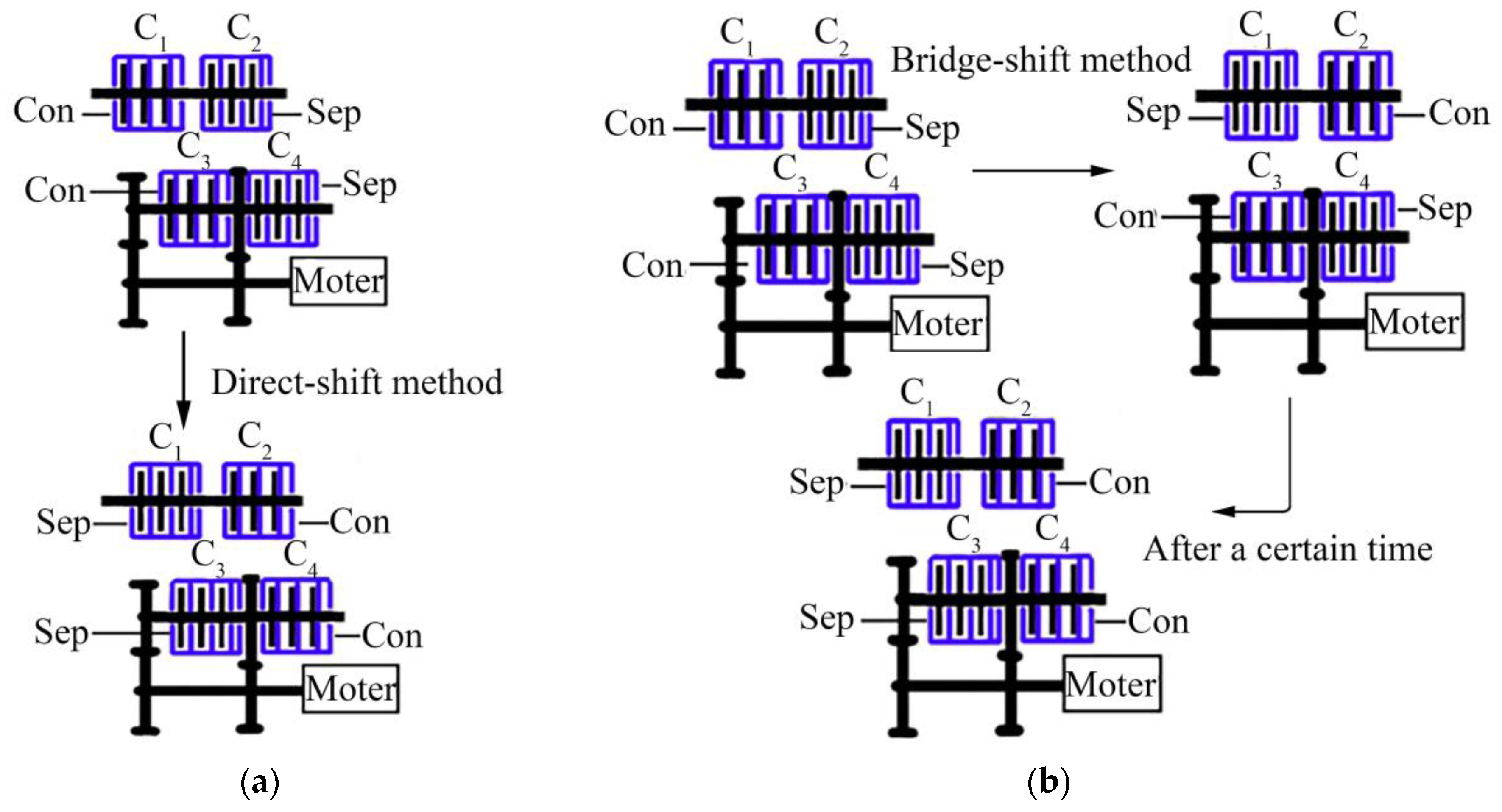
2.2. Control Strategies

The transmission involves the separation or engagement of four clutches during shifting, and the action timing of each clutch will have a significant impact on the shifting process. For example, after the separation of clutches C₁ and C₃, the speed of the tractor will continuously decrease under the action of the load. If the engagement of clutches C₂ and C₄ is slow, the driving and driven plates of the clutch will be in a continuous sliding state, which will burden the cooling system and shorten the service life of the clutch. In severe cases, it can also directly cause power interruption. On the contrary, if the engagement of clutches C₂ and C₄ is very fast, the speed difference between the driving and driven plates of the clutch is quickly eliminated, which will cause severe speed oscillations and significantly reduce the riding comfort of the tractor. The actual shifting process is very complex, which requires precise control of the actions of each clutch in the time domain. To solve this problem, two shifting strategies are proposed: the direct-shift and bridge-shift strategies.

Taking the switching of range HM₁ to range HM₂ as an example, the former separates clutches C₁ and C₃ while directly engaging clutches C₂ and C₄, while the latter needs to insert a transitional state of C₂ and C₃ engagement during the aforementioned process, as shown in Figure 2.

2.3. Modeling of the Swash Plate Axial Piston Units

The swash plate axial piston units are the core speed-regulating components of the CVT, consisting of a variable-displacement pump and a fixed-displacement motor. Its pressure, torque, flow, and speed meet the following equations:

$$T_p=\frac{e\mathsf{\Delta }{P}_p{V}_p}{2\pi }$$

(1)

$$T_m=\frac{{\mathsf{\Delta }P}_m{V}_m}{2\pi }$$

(2)

$$Q_p=\frac{e{V}_p{n}_p}{1000}$$

(3)

$$Q_m=\frac{V_m{n}_m}{1000}$$

(4)

where T_p and T_m are the theoretical torques of the pump shaft and motor shaft, respectively, N·m; ΔP_p and ΔP_m are the pressure differences between the inlet and outlet of the pump and motor, respectively, MPa; Q_p and Q_m are the theoretical flows of the pump and motor, respectively, L/min; n_p and n_m are the rotation speeds of the pump shaft and motor shaft, respectively, r/s; V_p and V_m are the rated displacements of the pump and motor, respectively, cm³/r; and e is the displacement ratio of the pump to the motor.

In actual systems, it is necessary to consider the torque loss and flow loss caused by mechanical friction and oil leakage:

$$T_{pr}=\frac{T_p}{{\eta }_{mp}}$$

(5)

$$T_{mr}=T_m{\eta }_{mm}$$

(6)

$$Q_{pr}=Q_p{\eta }_{vp}$$

(7)

$$Q_{mr}=\frac{Q_m}{{\eta }_{vm}}$$

(8)

where T_pr and T_mr are the real torques of the pump shaft and motor shaft, respectively, N·m; η_mp and η_mm are the mechanical efficiencies of the pump and motor, respectively; Q_pr and Q_mr are the real flows of the pump and motor, respectively, L/min; and η_vp and η_vm are the volume efficiencies of the pump and motor, respectively.

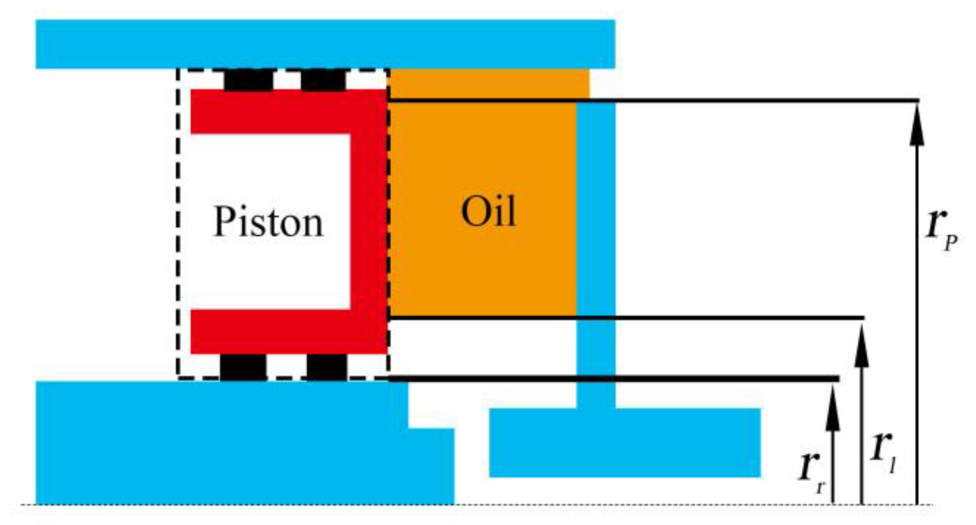
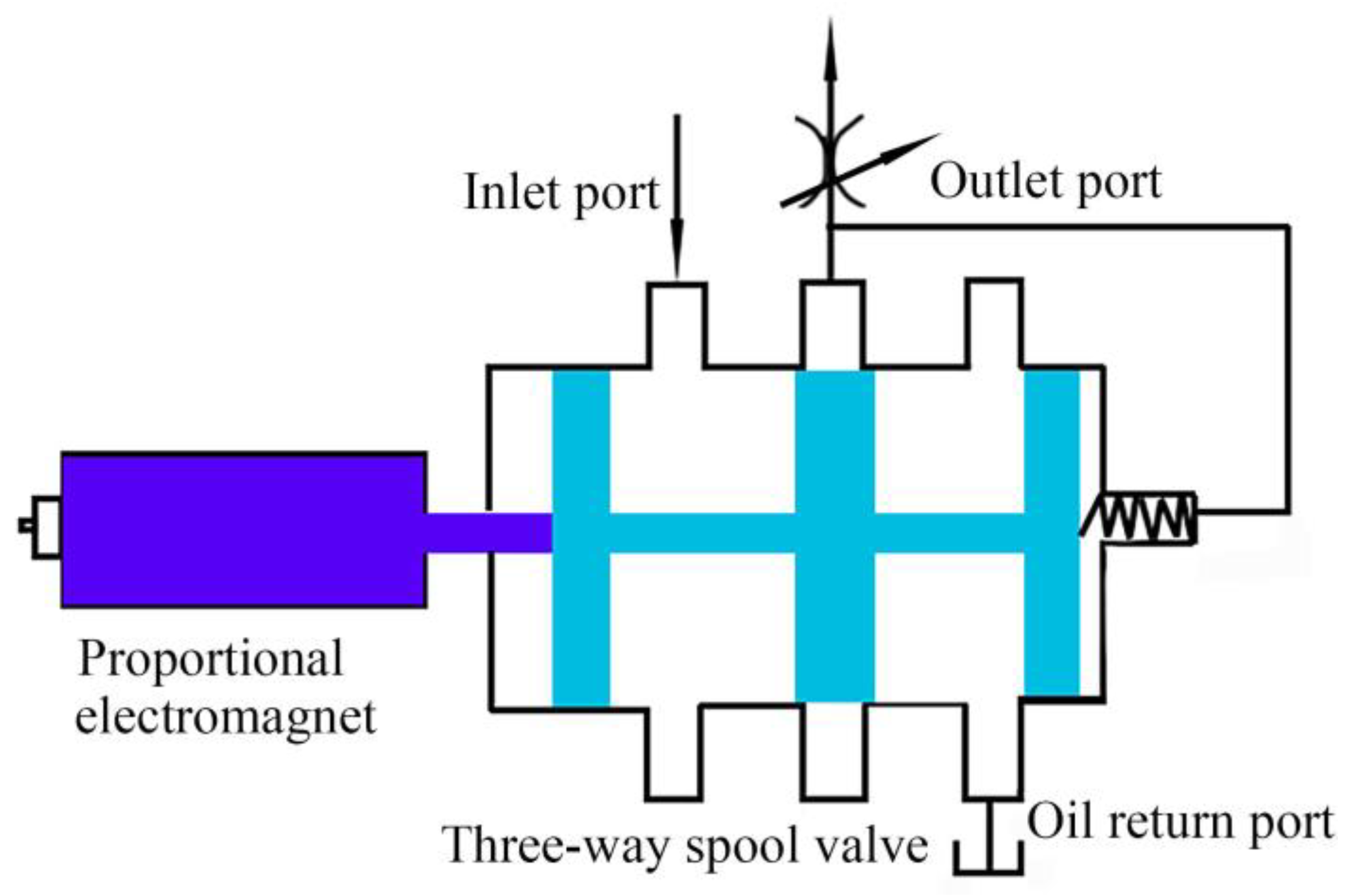
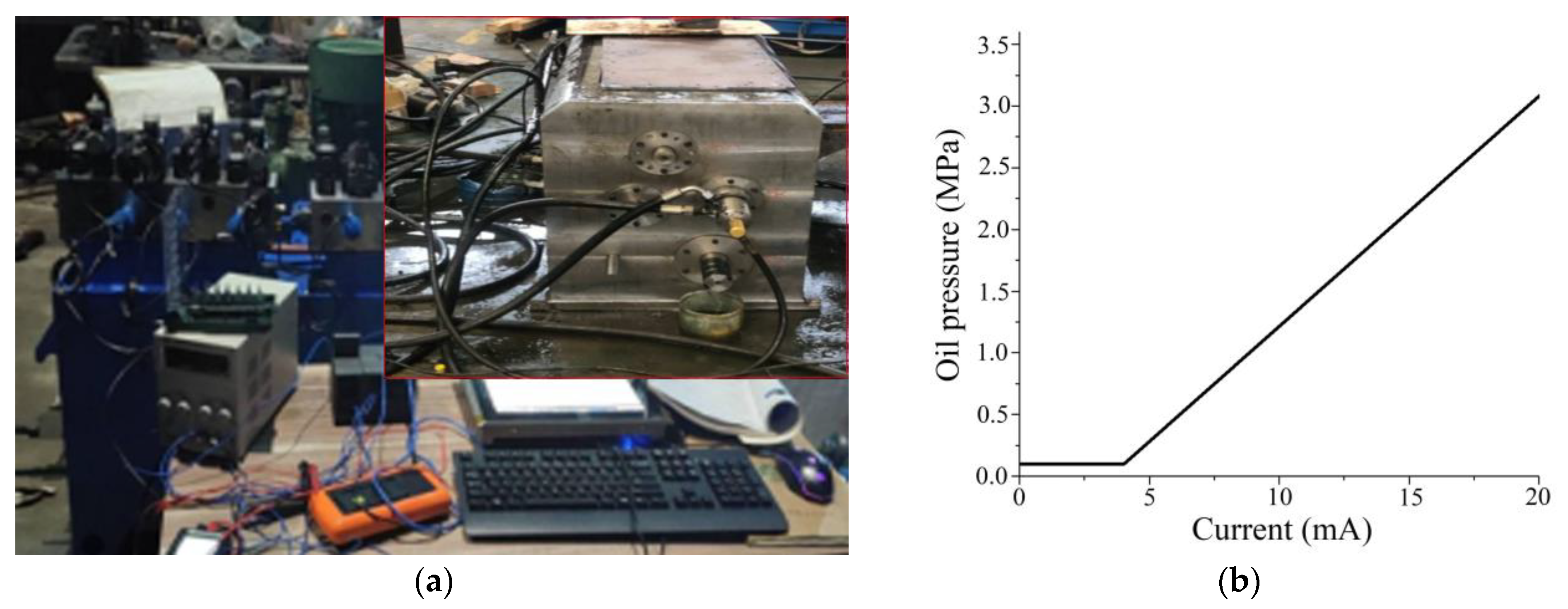
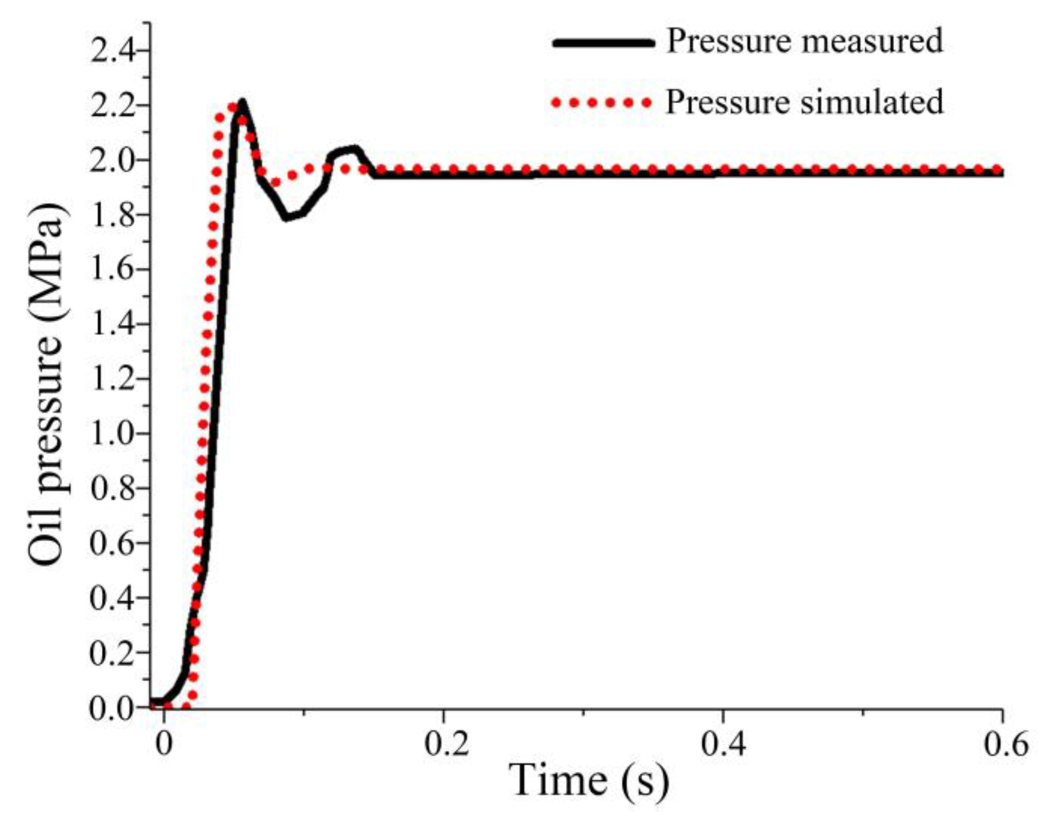
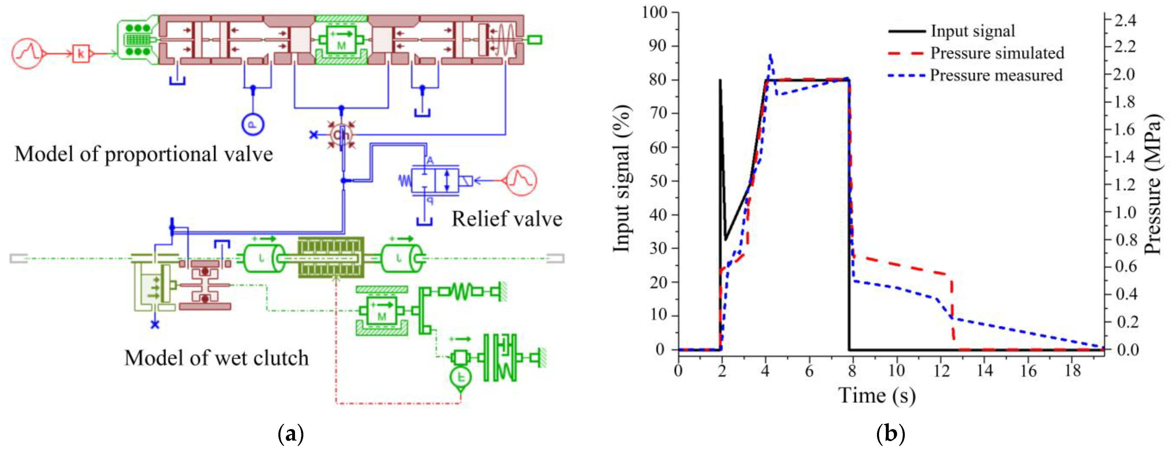
2.4. Modeling of the Power-Shift System

The power-shift system consists of wet clutches and a corresponding hydraulic circuit. The frictional torque that the clutch can transmit is:

$$T_c=\mu F_n{n}_p\times \frac{2\left(r_o^3-r_i^3\right)}{3\left(r_o^2-r_i^2\right)}\tanh \left(2\times \frac{R_n}{d_v}\right)$$

(9)

where T_c is the frictional torque transmitted in the clutch plates, N; μ is the coulomb friction coefficient; F_n is the normal force acting on the clutch plates, N; n_p is the number of clutch contact faces; r_o and r_i are the outside radius and inside radius of the friction plates, respectively, mm; R_n is the relative velocity, r/min; and d_v is the rotary stick velocity threshold, r/min.

The normal force F_n is determined by the combination of the oil pressure, centrifugal force, and spring force:

$$F_n=P_c{A}_c+F_c-k_c\left(x_{ci}+{\mathsf{\Delta }x}_c\right)$$

(10)

where P_c is the oil pressure, MPa; A_c is the effective area of the piston, mm²; F_c is the centrifugal force, N; k_c is the stiffness of the spring, N/mm; and x_ci and Δx_c are the initial compression and relative displacement of the spring, respectively, mm.

The rotary hydraulic cylinder is a typical coupling element used in multi-plate wet clutches in the transmission. Its rotational speed is high, so its oil chamber is subjected to centrifugal acceleration. The structure of the clutch hydraulic cylinder is shown in Figure 3, and the centrifugal force acting on its piston is calculated as follows:

$$F_c=\frac{\pi \rho {\omega }^2\left[r_p^4-r_r^4-2\times r_l^2\left(r_p^2-r_r^2\right)\right]}{4}$$

(11)

where ρ is the bulk density of the hydraulic oil, kg·m³; ω is the angular velocity, r/min; r_p and r_l are the outside radius and inside radius of the fluid volume acting on the piston, respectively, mm; and r_r is the inside radius of the piston, mm.

A proportional pressure valve is used to control the working pressure of the clutch, consisting of a proportional electromagnet and a three-way spool valve, as shown in Figure 4. When the electromagnetic force increases, the valve spool moves to the right to increase the opening of the outlet port, causing the output pressure to increase. When the electromagnetic force decreases, the valve spool moves to the left, causing the output pressure to decrease. On this basis, when the output pressure increases, the valve spool moves left to allow excess oil to flow back to the tank through the oil return port, thereby reducing the output pressure. When the output pressure decreases, the piston moves right to increase the output pressure. According to its working principle, the force equation of the valve spool is expressed as:

$$A_s{p}_{out}+F_{jet}+k_s\left(x_{si}+{\mathsf{\Delta }x}_s\right)=F_g$$

(12)

where A_s is the effective area of the valve spool, mm²; p_out is the output pressure of the valve, MPa; F_jet is the jet force, N; k_s is the stiffness of the spring, N/mm; x_si and Δx_s are the initial compression of the spring and the displacement of the valve spool, respectively, mm; and F_g is the electromagnetic force, N.

The jet force is calculated using the following equation:

$$F_{jet}=2C_q\pi d_s{\mathsf{\Delta }x}_s\left|{\mathsf{\Delta }p}_v\right|\cos {\alpha }_{jet}$$

(13)

where C_q is the flow coefficient; d_s is the equivalent diameter of the valve spool, mm; Δp_v is the pressure difference between the inlet and outlet of the valve, MPa; and α_jet is the jet angle, rad.

The displacement of the valve spool obtained by simultaneous Equations (12) and (13) is as follows:

$${\mathsf{\Delta }x}_s=\frac{F_g-A_s{p}_{out}-k_s{x}_{si}}{k_s+2C_q\pi d_s\left|{\mathsf{\Delta }p}_v\right|\cos {\alpha }_{jet}}$$

(14)

According to the above analysis, the output pressure of the proportional valve depends on the electromagnetic force F_g, which is controlled by a current signal. To clarify the corresponding relationship between the input current and output pressure, a signal generator is used to calibrate the valve, and the results are shown in Figure 5. It can be seen that within the current range of 4–20 mA, the input current of the proportional valve exhibits a clear linear relationship with oil pressure. Therefore, we used the calibration data to construct an electromagnetic model of the valve.

The hydraulic circuit constructed based on clutches and proportional valves is the core of the power-shift system and requires independent experimental verification of its mathematical model. We closed the outlet of the proportional valve before the experiment, and the PLC controlled its AD module to output a step signal corresponding to the rated pressure of the clutch. Note that the output signal of the AD module used was the voltage, which needed to be converted into a 4–20 mA current through a converter module to control the proportional valve. At the same time, the Labview program controlled the data acquisition card (NI USB-6009) to capture the output pressure of the proportional valve feedback from the sensor. The input signal of the simulation model was consistent with the experiment, that is, the input current was modulated from 0 to the maximum value in the experiment in a very short time to observe the pressure response of the model. The simulation and measurement results of the step response of the proportional pressure valve are shown in Figure 6. From the figure, it can be seen that the simulation results of the mathematical model constructed in this study were highly consistent with the experimental results and could meet the needs of subsequent dynamic analysis.

We connected the model of the proportional valve with the model of the wet clutch, further constructed the model of the power-shift system and conducted an experimental verification of it. The simulation and measurement results are shown in Figure 7. The figure shows that under the same input signal of the proportional valve, the clutch pressure response of the simulation model was basically consistent with the experimental results, thus proving the reliability of the constructed model.

The models of the proportional valve and wet clutch were relatively complex; for some models not covered in this article, please refer to the AMESim manual. The key parameters used in the simulation calculations are shown in

Table 2. Configuration parameters of proportional valves.

Input Signal/mA	Output Pressure/MPa	Spring Preload/N	Spring Stiffness/(N/mm)	Flow Coefficient	Mass of Spool/kg	Hole Diameter/mm
4~20	0~2	20.0	19.9	0.6	0.52	1.2

and

Table 3. Configuration parameters of wet clutches.

Clutch	Area of Friction Plate/(mm2)	Area of Piston/(mm2)	Number of Friction Plates	Spring Stiffness/(N/mm)	Frictional Coefficient
C1	7780	7210	7	19.6	0.12
C2	6900	6090	8	10.42	0.11
C3/C4	4780	3810	7	6.7	0.08

.

2.5. Modeling of Gears and Shafts

The torque and speed of the two meshing gears satisfy the following equations:

$$n_2=\frac{n_1}{i_{12}}$$

(15)

$$T_2=i_{12}{T}_1$$

(16)

where i₁₂ is the transmission ratio of the gear pairs; n₁ and n₂ are the speeds of the two gears, r/min; and T₁ and T₂ are the torques of the two gears, N·m.

The speed and torque between the three basic components of the planetary gear, the sun gear, the ring gear, and the carrier satisfy the following equations:

$$n_s+k{n}_r-\left(1+k\right)n_c=0$$

(17)

$$T_s:T_r:T_c=1:k:\left(1+k\right)$$

(18)

where n_s, n_r, and n_c are the speeds of the sun gear, ring gear, and carrier, respectively, r/min; T_s, T_r, and T_c are the torques of the sun gear, ring gear, and carrier, respectively, N·m; and k is the standing ratio of the standard planetary gear.

In this study, the moment of inertia of each component is calculated by the SolidWorks 2016 software and is equivalent to the transmission shaft. Its influence on the torque of each shaft is as follows:

$$T_a=T_0+J\frac{d\omega }{dt}$$

(19)

where T_a and T₀ are the actual torque and theoretical torque of the shaft, respectively, N·m; J is the moment of inertia, kg·m²; ω is the angular velocity of the shaft, rad/s; and t is the time, s.

2.6. Modeling of Tractor

Based on the above equations, a shift dynamics model of the entire continuously variable transmission tractor was constructed using AMESim, as shown in Figure 8.

3. Results and Discussion

3.1. Evaluation Indicators

The speed drop is defined as the difference between the output speed of the transmission before the shift and the lowest output speed during the shift:

$${\delta }_1={\omega }_1-{\omega }_2$$

(20)

where δ₁ is the speed drop, r/min; ω₁ is the output speed before the shift, r/min; and ω₂ is the lowest output speed during the shift, r/min.

According to Duncan and Wegscheid [23], the peak acceleration of a tractor in the longitudinal direction can well reflect its driving comfort during shifting. Therefore, this study took the peak acceleration as one of the indicators for evaluating the shifting quality of the CVT, and its expression is as follows:

$${\delta }_2=\mathrm{m}\mathrm{a}\mathrm{x}\left(\frac{dv}{dt}\right)$$

(21)

where δ₂ is the peak acceleration of the tractor during the shift, m/s².

When the clutch is engaged, a large amount of heat will be generated due to friction, and in severe cases, it may burn out the clutch. The power loss during the aforementioned process is as follows:

$${\delta }_3=\mathrm{m}\mathrm{a}\mathrm{x}\left(\frac{T_c\left|\mathsf{\Delta }\omega \right|}{9550}\right)$$

(22)

where δ₃ is the maximum power loss during the shift, kW; T_c is the friction torque, N·m; and Δω is the difference in the angular speed of the clutch driving and driven disc, r/min.

On this basis, sliding friction work is defined as the integral of the power loss over time:

$${\delta }_4={\int }_{t_1}^{t_2}\frac{T_c\left|\mathsf{\Delta }\omega \right|}{9550}dt$$

(23)

where δ₄ is the sliding friction work, kJ; and t₁ and t₂ are the start and end times of the shift, s.

3.2. Direct-Shift Method

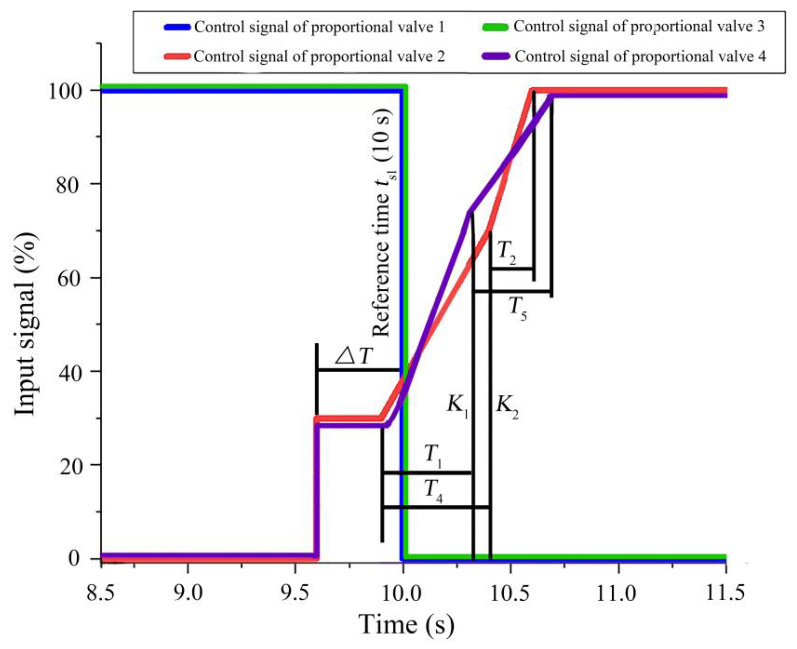
3.2.1. Determination of Shift Points

The process of direct shifting is relatively simple, with clutches C₁ and C₃ being separate while clutches C₂ and C₄ engage. During the shift process, the displacement ratio is synchronously adjusted, and its initial and final values need to meet the following relationship:

$$i_{\mathrm{H}\mathrm{M}1}=\frac{i_1{i}_2{i}_4{i}_6\left(1+k\right)}{k{i}_1{i}_4+e{i}_2{i}_6}$$

(24)

$$i_{\mathrm{H}\mathrm{M}2}=\frac{i_1{i}_3{i}_5{i}_6\left(1+k\right)}{k{i}_1{i}_5+e{i}_3{i}_6}$$

(25)

$$i_{\mathrm{H}\mathrm{M}1}=i_{\mathrm{H}\mathrm{M}2}$$

(26)

where i_HM1 and i_HM2 are the transmission ratios in HM₁ and HM₂, respectively; and i_x is the transmission ratio of the gear pair g_x.

From the perspective of transmission efficiency and energy consumption, the authors have demonstrated in previous research that the optimal shift point for this CVT in the range HM₁ is e = 1. Based on the above equations, the displacement ratio after the shift was calculated to be e = −0.8034.

3.2.2. Optimization of Shifting Quality

The pressure control signal of the proportional valve based on the direct-shift method is shown in Figure 9. If we define the pressure relief time of proportional valves 1 and 3 as t_s1 (i.e., reference time, 10 s), then ΔT is the start time of the pressure rise for proportional valves 2 and 4 relative to t_s1. T₄ and T₂ are the times corresponding to the two inflection points in the pressure rise curve of proportional valve 2, respectively. T₁ and T₅ are the times corresponding to the two inflection points in the pressure rise curve of proportional valve 4, respectively. K₂ and K₁ are the percentages of the input signals corresponding to the second inflection point in the pressure rise curve of proportional valves 2 and 4, respectively. The starting time of T₁ and T₄ is the same, and the starting time and duration of the reverse change in the displacement ratio are T_s and T_d, respectively. On this basis, we adopted an orthogonal experiment with nine factors and four levels to optimize the above control parameters. The schedule of the experiment is shown in

Table 4. Factors and levels used for direct-shift optimization.

Level	T1/ms	T2/ms	K1/%	T4/ms	T5/ms	K2/%	ΔT/ms	Ts/s	Td/ms
1	200	400	40	200	400	40	350	9.9	500
2	250	500	50	250	500	50	400	10	650
3	300	600	60	300	600	60	450	10.1	800
4	350	700	70	350	700	70	500	10.2	950

, and the results are shown in

Table 5. Orthogonal simulation sequence for direct-shift optimization.

	Factor	A	B	C	D	E	F	G	H	I	Peak Acceleration
Number
Test 1		1	1	1	1	1	1	1	1	1	2.754091
Test 2		1	2	2	2	2	2	2	2	2	2.218880
Test 3		1	3	3	3	3	3	3	3	3	0.746190
Test 4		1	4	4	4	4	4	4	4	4	1.523540
Test 5		2	1	1	2	2	3	3	4	4	1.526142
Test 6		2	2	2	1	1	4	4	3	3	1.028317
Test 7		2	3	3	4	4	1	1	2	2	2.135518
Test 8		2	4	4	3	3	2	2	1	1	2.862647
Test 9		3	1	2	3	4	1	2	3	4	1.061769
Test 10		3	2	1	4	3	2	1	4	3	0.627891
Test 11		3	3	4	1	2	3	4	1	2	3.136779
Test 12		3	4	3	2	1	4	3	2	1	0.614615
Test 13		4	1	2	4	3	3	4	2	1	2.631731
Test 14		4	2	1	3	4	4	3	1	2	3.048925
Test 15		4	3	4	2	1	1	2	4	3	1.001010
Test 16		4	4	3	1	2	2	1	3	4	0.674891
Test 17		1	1	4	1	4	2	3	2	3	1.952227
Test 18		1	2	3	2	3	1	4	1	4	2.758566
Test 19		1	3	2	3	2	4	1	4	1	0.501519
Test 20		1	4	1	4	1	3	2	3	2	0.814421
Test 21		2	1	4	2	3	4	1	3	2	0.627852
Test 22		2	2	3	1	4	3	2	4	1	0.584379
Test 23		2	3	2	4	1	2	3	1	4	2.766946
Test 24		2	4	1	3	2	1	4	2	3	1.894956
Test 25		3	1	3	3	1	2	4	4	2	0.901438
Test 26		3	2	4	4	2	1	3	3	1	1.022129
Test 27		3	3	1	1	3	4	2	2	4	1.486624
Test 28		3	4	2	2	4	3	1	1	3	2.839502
Test 29		4	1	3	4	2	4	2	1	3	2.871530
Test 30		4	2	4	3	1	3	1	2	4	1.853240
Test 31		4	3	1	2	4	2	4	3	1	0.999228
Test 32		4	4	2	1	3	1	3	4	2	0.398879

and

Table 6. Range analysis of orthogonal optimization for direct-shift strategy.

Factor	T1	T2	K1	T4	T5	K2	ΔT	Ts	Td
1	1.569	1.791	1.644	1.502	1.467	1.628	1.502	2.880	1.496
2	1.678	1 643	1.681	1.573	1.731	1.626	1.613	1.848	1.660
3	1.461	1.597	1.411	1.609	1 518	1.767	1.510	0.872	1.620
4	1.685	1.453	1.747	1.799	1.768	1.463	1.859	0.883	1.706
Range	0.224	0.338	0.336	0.297	0.301	0.304	0.357	2.008	0.210

. Considering that the peak acceleration directly affects the driving comfort, we only optimized the parameters for this indicator when designing the orthogonal experiments, but we considered other indicators together when analyzing the results.

According to the results of the orthogonal range analysis, when switching from HM₁ to HM₂, the degree of influence of each factor on the direct-shift method was ranked as follows: the reverse starting point T_s, the time difference ΔT, time T₂, current K₁, current K₂, time T₅, time T₄, time T₁, and the reverse duration T_d. The best combination of factors was A₃B₄C₃D₁E₁F₄G₃H₃I₁. By substituting the optimized parameters into the simulation model, the various indicators for the direct-shift method were obtained as follows: the speed drop was 30.67 r/min (no power interruption), the peak acceleration was 0.384535 m/s², the power loss of clutch C₂ was 22.7383 kW, the sliding friction work of clutch C₂ was 8.0752 kJ, the power loss of clutch C₄ was 18.1166 kW, and the sliding friction work of clutch C₄ was 2.3906 kJ.

3.3. Bridge-Shift Method

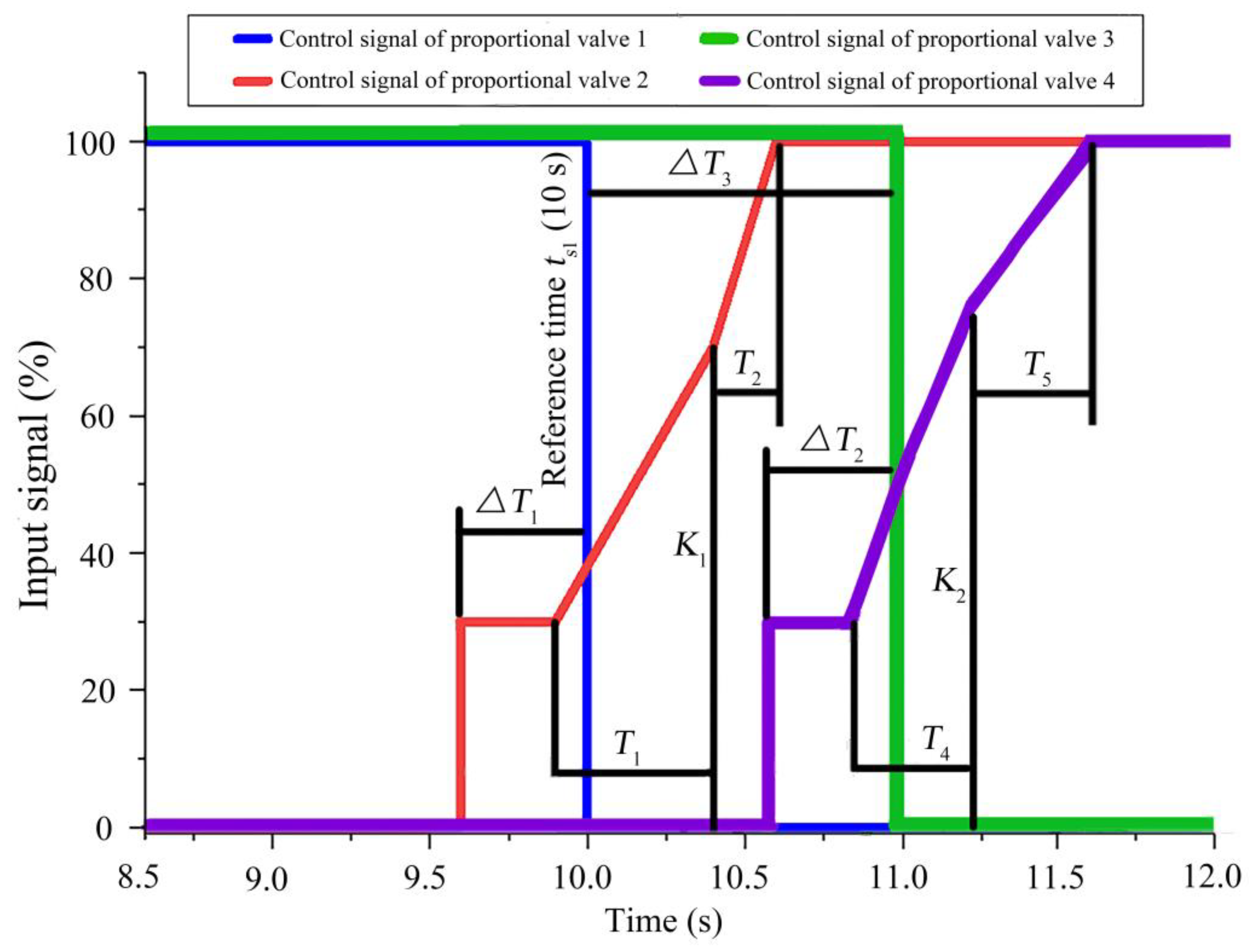
3.3.1. Determination of Shift Points

The process of bridge shifting is divided into two stages. In the first stage, the transmission shifts from the low-speed range HM₁ to the transition range, where clutch C₁ separates while clutch C₂ engages. In the second stage, the transmission shifts from the transition range to the high-speed range HM₂, where clutch C₃ separates and clutch C₄ engages. During the shift process, the displacement ratio is synchronously adjusted, and its initial and final values are the same as those of the direct-shift method. However, the displacement ratio of the transition range will be used as an optimization variable, which will be discussed later.

3.3.2. Optimization of Shifting Quality

The pressure control signal of the proportional valve based on the bridge-shift method is shown in Figure 10. The factors T₁, T₂, K₁, T₄, T₅, and K₂ in the bridge-shift method are the same as those specified in the direct-shift method. We define the pressure relief times for proportional valves 1 and 3 as t_s1 (10 s) and t_s2 (10 s + ΔT₃), respectively; then, ΔT₁ is the start time of the pressure increase for proportional valve 2 relative to t_s1. ΔT₂ is the start time of the pressure increase for proportional valve 4 relative to t_s2. The starting time of the reverse change in displacement ratio is T_s. The duration of the two stages of the reverse change in the displacement ratio are T_d1 and T_d2, respectively. The displacement ratio of the transition range is e_t. On this basis, we adopted an orthogonal experiment with thirteen factors and three levels to optimize the above control parameters. The schedule of the experiment is shown in

Table 7. Factors and levels used for bridge-shift optimization.

Level	T1/ms	T2/ms	K1/%	T4/ms	T5/ms	K2/%	ΔT1/ms	ΔT2/ms	ΔT3/ms	Ts/s	Td1/ms	Td2/ms	et/s
1	250	500	50	250	500	50	400	400	500	9.9	150	350	−1
2	300	600	60	300	600	60	450	450	750	10	200	500	−0.95
3	350	700	70	350	700	70	500	500	1000	10.1	250	650	−0.9

, and the results are shown in

Table 8. Orthogonal simulation sequence for bridge-shift optimization.

	Factor	A	B	C	D	E	F	G	H	I	J	K	L	M	Peak Acceleration
Number
Test 1		1	1	1	1	1	1	1	1	1	1	1	1	1	2.693358
Test 2		1	1	1	1	2	2	2	2	2	2	2	2	2	2.655476
Test 3		1	1	1	1	3	3	3	3	3	3	3	3	3	1.527961
Test 4		1	2	2	2	1	1	1	2	2	2	3	3	3	1.152763
Test 5		1	2	2	2	2	2	2	3	3	3	1	1	1	1.169344
Test 6		1	2	2	2	3	3	3	1	1	1	2	2	2	2.620924
Test 7		1	3	3	3	1	1	1	3	3	3	2	2	2	0.986310
Test 8		1	3	3	3	2	2	2	1	1	1	3	3	3	2.600973
Test 9		1	3	3	3	3	3	3	2	2	2	1	1	1	1.178958
Test 10		2	1	2	3	1	2	3	2	2	3	1	2	3	0.840597
Test 11		2	1	2	3	2	3	1	2	3	1	2	3	1	2.284741
Test 12		2	1	2	3	3	1	2	3	1	2	3	1	2	1.072096
Test 13		2	2	3	1	1	2	3	2	3	1	3	1	2	2.606293
Test 14		2	2	3	1	2	3	1	3	1	2	1	2	3	1.374078
Test 15		2	2	3	1	3	1	2	1	1	3	2	3	1	1.139140
Test 16		2	3	1	2	1	2	2	3	1	2	2	3	1	1.244164
Test 17		2	3	1	2	2	3	3	1	2	3	3	1	2	0.545924
Test 18		2	3	1	2	3	1	1	2	3	1	1	2	3	2.701621
Test 19		3	1	3	2	1	3	2	1	3	2	1	3	2	1.371793
Test 20		3	1	3	2	2	1	3	2	1	3	2	1	3	0.451569
Test 21		3	1	3	2	3	2	1	3	2	1	3	2	1	2.626360
Test 22		3	2	1	3	1	3	2	2	1	3	3	2	1	0.417362
Test 23		3	2	1	3	2	1	3	3	2	1	1	3	2	2.697961
Test 24		3	2	1	3	3	2	1	1	3	2	2	1	3	1.339399
Test 25		3	3	2	1	1	3	2	3	2	1	2	1	3	2.665314
Test 26		3	3	2	1	2	1	3	1	3	2	3	2	1	1.008765
Test 27		3	3	2	1	3	2	1	2	1	3	1	3	2	0.411107

and

Table 9. Range analysis of orthogonal optimization for bridge-shift strategy.

Factor	T1/ms	T2/ms	K1/ms	T4/ms	T5	K2	ΔT1	ΔT2	ΔT3	Ts	Td1	Td2	et
1	1.843	1.726	1.758	1.787	1.553	1.545	1.492	1.573	1.432	2.612	1.604	1.525	1.530
2	1.535	1.613	1.471	1.543	1.644	1.722	1.755	1.541	1.722	1.378	1.711	1.692	1.663
3	1.443	1.483	1.593	1.492	1.624	1.555	1.575	1.707	1.667	0.832	1.506	1.605	1.628
Range	0.400	0.243	0.287	0.295	0.091	0.177	0.263	0.166	0.290	1.780	0.205	0.167	0.133

.

According to the results of the orthogonal range analysis, when switching from HM₁ to HM₂, the degree of influence of each factor with the bridge-shift method was ranked as follows: the reverse starting point T_s, time T₁, time T₄, time difference ΔT₃, current K₁, time difference ΔT₁, time T₂, the reverse duration T_d1, the reverse duration T_d2, current K₂, time difference ΔT₂, displacement ratio e_t, and time T₅. The optimum level combination was A₃B₃C₂D₃E₁F₁G₁H₂I₁J₃K₃L₁M₁, and after substituting the parameters into the simulation model, the various indicators for the bridge-shift method were obtained as follows: the speed drop was 16.035 r/min (no power interruption), the peak acceleration was 0.385807 m/s², the power loss of clutch C₂ was 17.5495 kW, the sliding friction work of clutch C₂ was 6.8700 kJ, the power loss of clutch C₄ was 4.6241 kW, and the sliding friction work of clutch C₄ was 0.5775 kJ.

The shifting results under the two control strategies are shown in Figure 11. Compared to the direct-shift method, the shifting quality of the tractor based on the bridge-shift method was greatly improved: the speed drop was reduced by 47.72%, the peak acceleration was increased by 0.33% (which can be ignored), the power loss of clutch C₂ was reduced by 22.82%, the sliding friction work of clutch C₂ was reduced by 14.92%, the power loss of clutch C₄ was reduced by 74.48%, and the sliding friction work of clutch C₄ was reduced by 75.84%.

3.4. Discussion

Due to the involvement of multiple clutch actions, the generation of parasitic power is inevitable. To determine the direction of the power flow, we observed the power loss of all the clutches during shifting, as shown in Figure 12a,b. The figure shows that in the direct-shift method, parasitic power mainly flowed back along clutch C₃, while in the bridge-shift method, parasitic power mainly flowed back along clutch C₁. However, compared to the power flowing in the forward direction in clutches C₂ and C₄, the parasitic power generated under both shifting strategies was not significant, so the energy loss of clutches C₁ and C₃ was not discussed in this study.

Tractors can operate within a larger range of loads, so it was necessary to further analyze the shifting quality of the tractor under different tractive forces, as shown in Figure 13.

From Figure 13a,b, it can be seen that when the tractive force was less than 20,000 N, the speed drop and peak acceleration both rapidly decreased with the increase in the load. When the tractive force was greater than 20,000 N, the speed drop no longer changed significantly, while the peak acceleration still decreased slightly with the increase in the load. Figure 13c shows that the power loss of clutch C₄ decreased with increasing the load, while the variation law of clutch C₂ was opposite. However, the above law was very insignificant, especially since the variation in clutch C₂ with the load was very small. Figure 13d shows that the sliding friction work of clutch C₂ increased with increasing the load, while clutch C₄ showed the same law but was not significant.

In response to the above laws, we provide the following explanation: the speed impact and energy losses were mutually affected and formed a causal relationship, that is, the clutch absorbed the speed and acceleration impact of the transmission system through its sliding process. Therefore, the load reduced the speed impact, and its cost was the severe sliding of the clutch friction plates and high energy losses.

In addition, by comparing the response of the two shifting strategies to the load, it was found that bridge-shift method had a significantly lower speed drop, power loss, and sliding friction work than the direct-shift method, except for its peak acceleration, which was comparable to that of the direct-shift method. It should be further emphasized that the tractor did not experience power interruption in all the simulation results. Therefore, the bridge-shift method proposed in this study is widely applicable to various load conditions of tractors.

4. Conclusions

This study conducted a shift dynamics analysis of a hydrostatic power-split tractor transmission with a single standard planetary gear set. Two power-shift strategies were proposed and compared, and the conclusions obtained are as follows:

(1)

The degree of influence of each factor with the direct-shift method is ranked as follows: the reverse starting point T_s, the time difference ΔT, time T₂, current K₁, current K₂, time T₅, time T₄, time T₁, and the reverse duration T_d. The best combination of factors is A₃B₄C₃D₁E₁F₄G₃H₃I₁.

(2)

The degree of influence of each factor with the bridge-shift method is ranked as follows: the reverse starting point T_s, time T₁, time T₄, time difference ΔT₃, time difference ΔT₁, time T₂, the reverse duration T_d1, time difference ΔT₂, displacement ratio e_t, swash plate axial piston unit’s reversal start point, current K₂, the reverse duration T_d2, and time T₅. The optimum level combination is A₃B₃C₂D₃E₁F₁G₁H₂I₁J₃K₃L₁M₁.

(3)

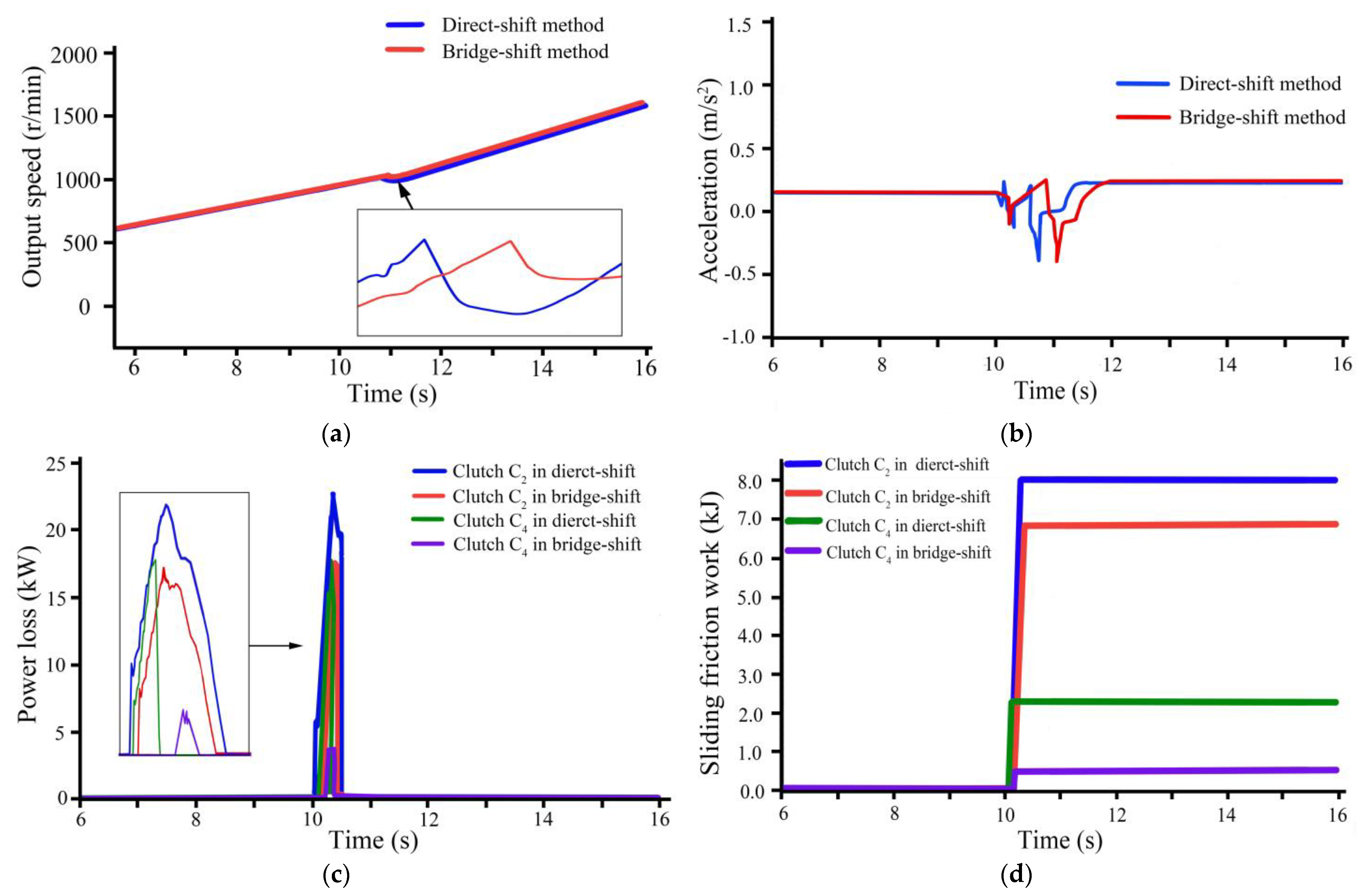
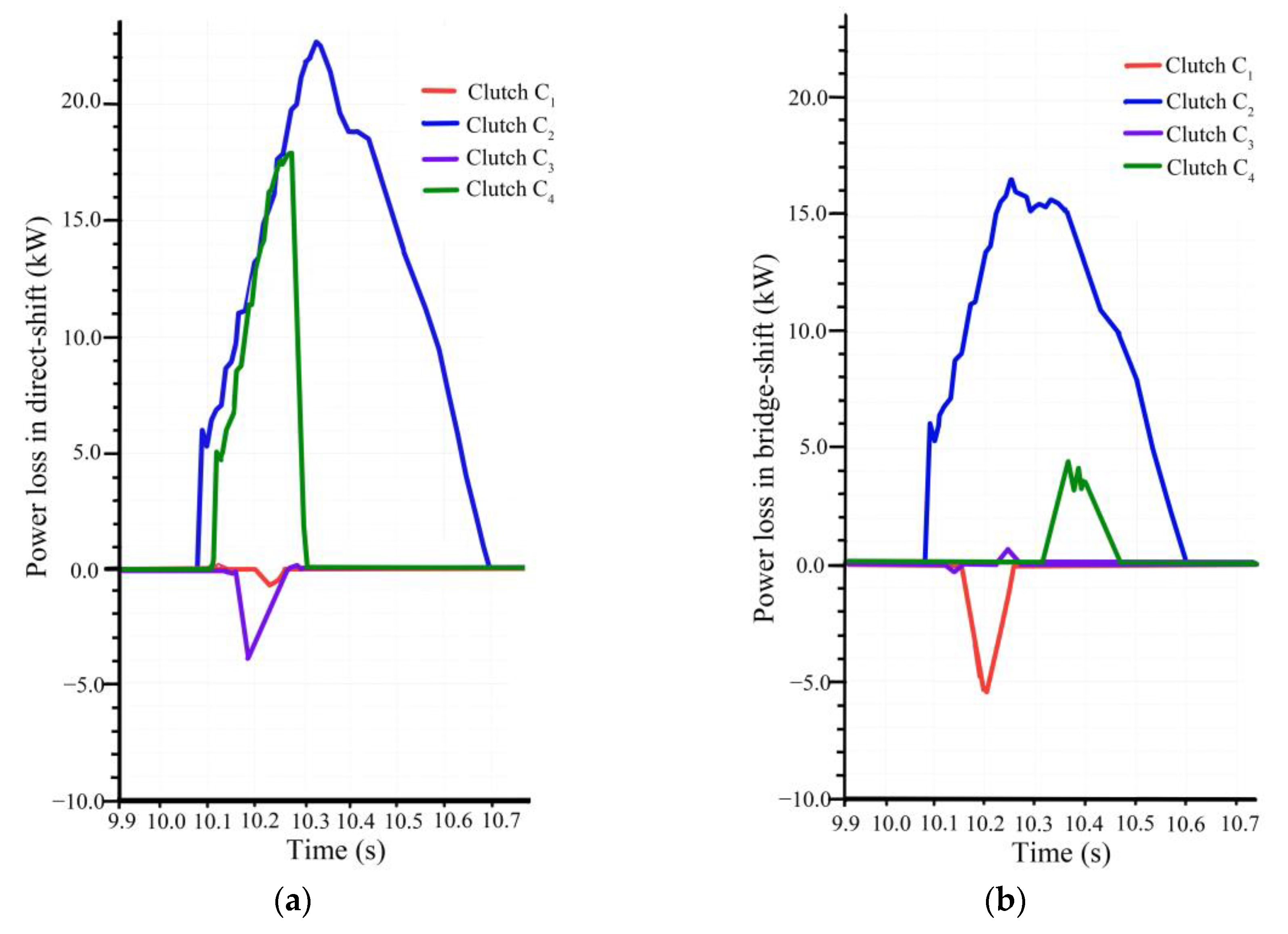
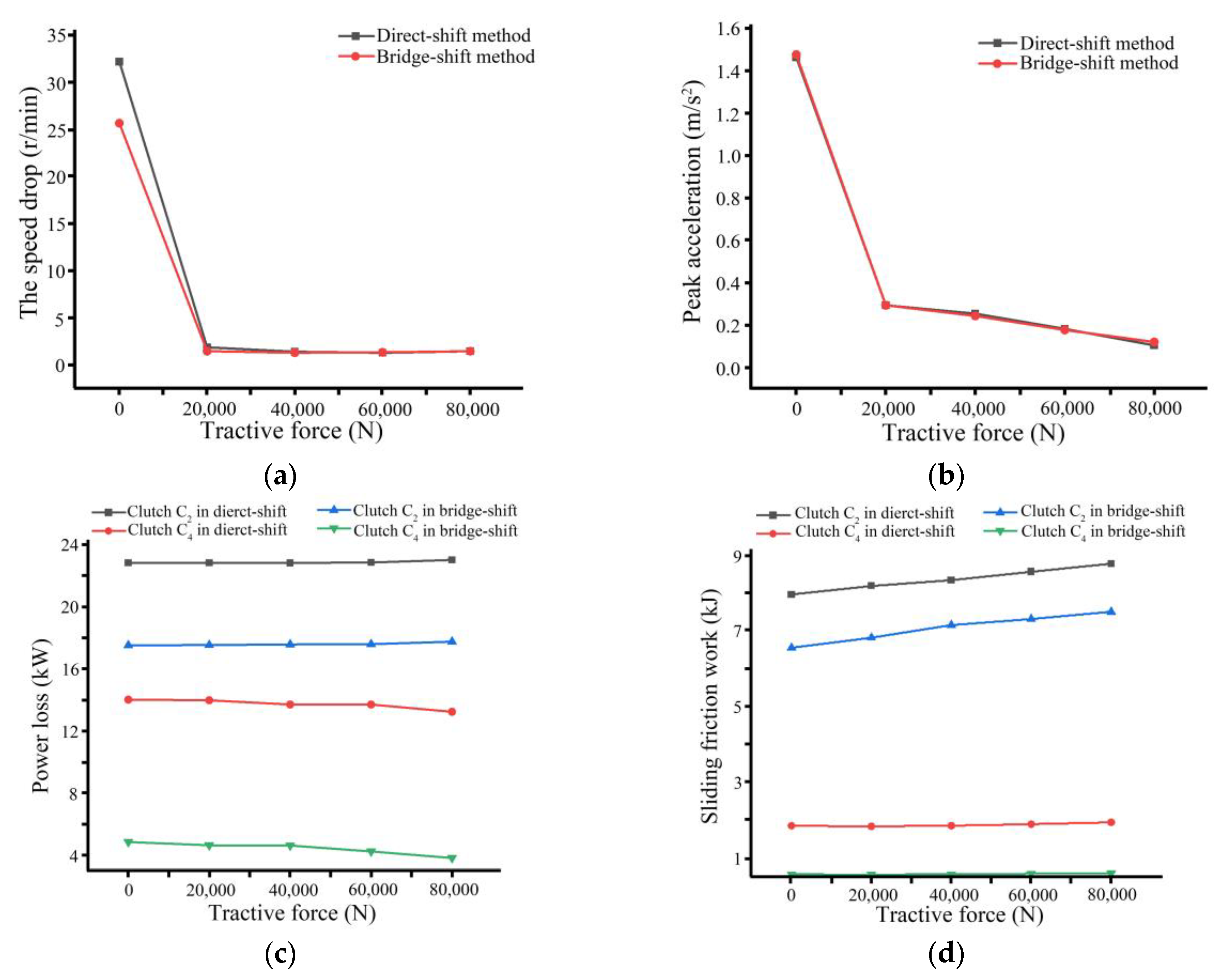
Compared with the direct-shift method, the bridge-shift method reduces the speed drop by 47.72%, the power loss of clutch C₂ by 22.82%, the sliding friction work of clutch C₂ by 14.92%, the power loss of clutch C₄ by 74.48%, and the sliding friction work of clutch C₄ by 75.84%. In addition, the influence of the two control strategies on the peak acceleration can be ignored.

(4)

Under different tractive forces, the quality of the bridge-shift method is better than that of the direct-shift method, and no power interruption phenomenon was observed in all the simulation calculations.

References

1. Guo, X.; Vacca, A. Advanced design and optimal sizing of hydrostatic transmission systems. Actuators 2021, 10, 243. [Google Scholar] [CrossRef]
2. Dario, R.; Macro, C. Power losses in power-split CVTs: A fast black-box approximate method. Mech. Mach. Theory 2018, 128, 528–543. [Google Scholar] [CrossRef]
3. Kim, J.Y.; Bae, D.S. Development of 3D dynamic and 1D numerical model for computing pulley ratio of chain CVT transmission. Int. J. Auto. Technol. 2022, 23, 1045–1053. [Google Scholar] [CrossRef]
4. Chen, Y.; Cheng, Z.; Qian, Y. Fuel consumption comparison between hydraulic mechanical continuously variable transmission and stepped automatic transmission based on the economic control strategy. Machines 2022, 10, 699. [Google Scholar] [CrossRef]
5. İnce, E.; Güler, M.A. On the advantages of the new power-split infinitely variable transmission over conventional mechanical transmissions based on fuel consumption analysis. J. Clean. Prod. 2020, 244, 118795. [Google Scholar] [CrossRef]
6. Zhang, M.; Wang, J.; Wang, J.; Guo, Z.; Guo, F.; Xi, Z.; Xu, J. Speed changing control strategy for improving tractor fuel economy. Trans. Chin. Soc. Agric. Eng. 2020, 36, 82–89. [Google Scholar]
7. Wang, G.; Zhao, Y.; Song, Y.; Xue, L.; Chen, X. Optimizing the fuel economy of hydrostatic power-split system in continuously variable tractor transmission. Heliyon 2023, 9, e15915. [Google Scholar] [CrossRef]
8. Renius, K.T. Fundamentals of Tractor Design; Springer Nature: Cham, Switzerland, 2020. [Google Scholar]
9. Renius, K.T.; Resch, R. Continuously variable tractor transmissions. In Proceedings of the 2005 Agriculture Equipment Technology Conference, Louisville, KY, USA, 14–16 February 2005. [Google Scholar]
10. Xia, Y.; Sun, D.; Qin, D.; Zhou, X. Optimisation of the power-cycle hydro-mechanical parameters in a continuously variable transmission designed for agricultural tractors. Biosyst. Eng. 2020, 193, 12–24. [Google Scholar] [CrossRef]
11. Liu, F.; Wu, W.; Hu, J.; Yuan, S. Design of multi-range hydro-mechanical transmission using modular method. Mech. Syst. Signal Process. 2019, 126, 1–20. [Google Scholar] [CrossRef]
12. Wang, J.; Xia, C.; Fan, X.; Cai, J. Research on transmission characteristics of hydromechanical continuously variable transmission of tractor. Math. Probl. Eng. 2020, 2020, 6978329. [Google Scholar] [CrossRef]
13. Li, B.; Pan, J.; Li, Y.; Ni, K.; Huang, W.; Jiang, H.; Liu, F. Optimization method of speed ratio for power-shift transmission of agricultural tractor. Machines 2023, 11, 438. [Google Scholar] [CrossRef]
14. Wang, J.; Xia, C.; Fan, X.; Cai, J. Research on the influence of tractor parameters on shift quality, based on uniform design. Appl. Sci. 2022, 12, 4895. [Google Scholar] [CrossRef]
15. Li, B.; Ni, K.; Li, Y.; Pan, J.; Huang, W.; Jiang, H.; Liu, F. Control strategy of shuttle shifting process of agricultural tractor during headland turn. IEEE Access 2023, 11, 38436–38447. [Google Scholar] [CrossRef]
16. Bao, M.; Ni, X.; Zhao, X.; Li, S. Research on the HMCVT gear shifting smoothness of the four-speed self-propelled cotton picker. Mech. Sci. 2020, 11, 267–283. [Google Scholar] [CrossRef]
17. Chen, Y.; Qian, Y.; Lu, Z.; Zhou, S.; Xiao, M.; Bartos, P.; Xiong, Y.; Jin, G.; Zhang, W. Dynamic characteristic analysis and clutch engagement test of HMCVT in the high-power tractor. Complexity 2021, 2021, 8891127. [Google Scholar] [CrossRef]
18. Iqbal, S.; Al-bender, F.; Ompusunggu, A.P.; Pluymers, B.; Desmet, W. Modeling and analysis of wet friction clutch engagement dynamics. Mech. Syst. Signal Process. 2015, 60–61, 420–436. [Google Scholar] [CrossRef]
19. Wang, G.; Xue, L.; Zhu, Y.; Zhao, Y.; Jiang, H.; Wang, J. Fault diagnosis of power-shift system in continuously variable transmission tractors based on improved Echo State Network. Eng. Appl. Artif. Intel. 2023, in press. [Google Scholar]
20. Xiang, Y.; Li, R.; Brach, C.; Liu, X.; Geimer, M. A novel algorithm for hydrostatic-mechanical mobile machines with a dual-clutch transmission. Energies 2022, 15, 2095. [Google Scholar] [CrossRef]
21. Li, G.; Görges, D. Optimal control of the gear shifting process for shift smoothness in dual-clutch transmissions. Mech. Syst. Signal Process. 2018, 103, 23–38. [Google Scholar] [CrossRef]
22. Li, J.; Dong, H.; Han, B.; Zhang, Y.; Zhu, Z. Designing comprehensive shifting control strategy of hydro-mechanical continuously variable transmission. Appl. Sci. 2022, 12, 5716. [Google Scholar] [CrossRef]
23. Duncan, J.R.; Wegscheid, E.L. Determinants of off-road vehicle transmission ‘shift quality’. Appl Ergon. 1985, 16, 173–178. [Google Scholar] [CrossRef] [PubMed]
Figure 1. Transmission scheme of hydrostatic power-split CVT. Note: the symbol g represents the gear pair, and the symbol C represents the wet clutch.
Agriculture 13 01685 g001
Figure 2. Shift process under different control strategies. (a) Direct-shift method. (b) Bridge-shift method.
Agriculture 13 01685 g002
Figure 3. Schematic diagram of the clutch hydraulic cylinder.
Agriculture 13 01685 g003
Figure 4. Schematic diagram of the proportional pressure valve.
Agriculture 13 01685 g004
Figure 5. Calibration of the proportional pressure valve. (a) Hydraulic system used for calibration testing. (b) Calibration results of the proportional valve.
Agriculture 13 01685 g005
Figure 6. Simulation and measurement results of step response of proportional pressure valve.
Agriculture 13 01685 g006
Figure 7. Experimental verification of the simulation model of the shift hydraulic system. (a) Simulation model of shift hydraulic system. (b) Simulation and measurement results of the response of clutch pressure to control signals. Note: the relief valve was designed for rapid pressure relief and was consistent with the actual hydraulic circuit.
Agriculture 13 01685 g007
Figure 8. Shifting dynamics model of continuously variable transmission tractor.
Agriculture 13 01685 g008
Figure 9. Pressure control signal of the clutch under direct-shift strategy. Note: considering that the rated pressure of the proportional valve and the clutch are not consistent, the input signal has been redefined here, with the maximum signal corresponding to the rated pressure of the clutch.
Agriculture 13 01685 g009
Figure 10. Pressure control signal of the clutch under bridge-shift strategy. Note: considering that the rated pressure of the proportional valve and the clutch are not consistent, the input signal has been redefined here, with the maximum signal corresponding to the rated pressure of the clutch.
Agriculture 13 01685 g010
Figure 11. Comparison of shifting quality under different control strategies. (a) Output speed of the transmission during shift. (b) Acceleration of the tractor during shift. (c) Power loss of the clutches during shift. (d) Sliding friction work of the clutches during shift.
Agriculture 13 01685 g011
Figure 12. Power loss of clutches. (a) Power loss in direct-shift method. (b) Power loss in bridge-shift method.
Agriculture 13 01685 g012
Figure 13. Shifting quality under different tractive forces. (a) Speed drop of the transmission during shifting. (b) Peak acceleration of the tractor during shifting. (c) Power loss of the clutches during shifting. (d) Sliding friction work of the clutches during shifting. Note: The clutch still loses energy under no load because the model takes into account the effects of cab air resistance and tire rolling resistance. Moreover, inertial loads can also cause energy losses.
Agriculture 13 01685 g013