Author Contributions
Conceptualization, S.M., A.O. and A.S.; methodology, O.P.B., C.S., S.M., A.O. and A.S.; software, O.P.B., C.S. and A.S.; validation, O.P.B., C.S. and A.S.; formal analysis, O.P.B., C.S., S.M., A.O. and A.S.; investigation, O.P.B., C.S., S.M., A.O. and A.S.; resources, O.P.B., C.S., S.M., A.O. and A.S.; data curation, O.P.B., C.S., S.M., A.O. and A.S.; writing—original draft preparation, O.P.B., C.S. and A.S.; writing—review and editing, O.P.B., C.S., S.M., A.O. and A.S.; visualization, O.P.B., C.S. and A.S.; supervision, A.S.; project administration, A.S.; funding acquisition, S.M., A.O. and A.S. All authors have read and agreed to the published version of the manuscript.
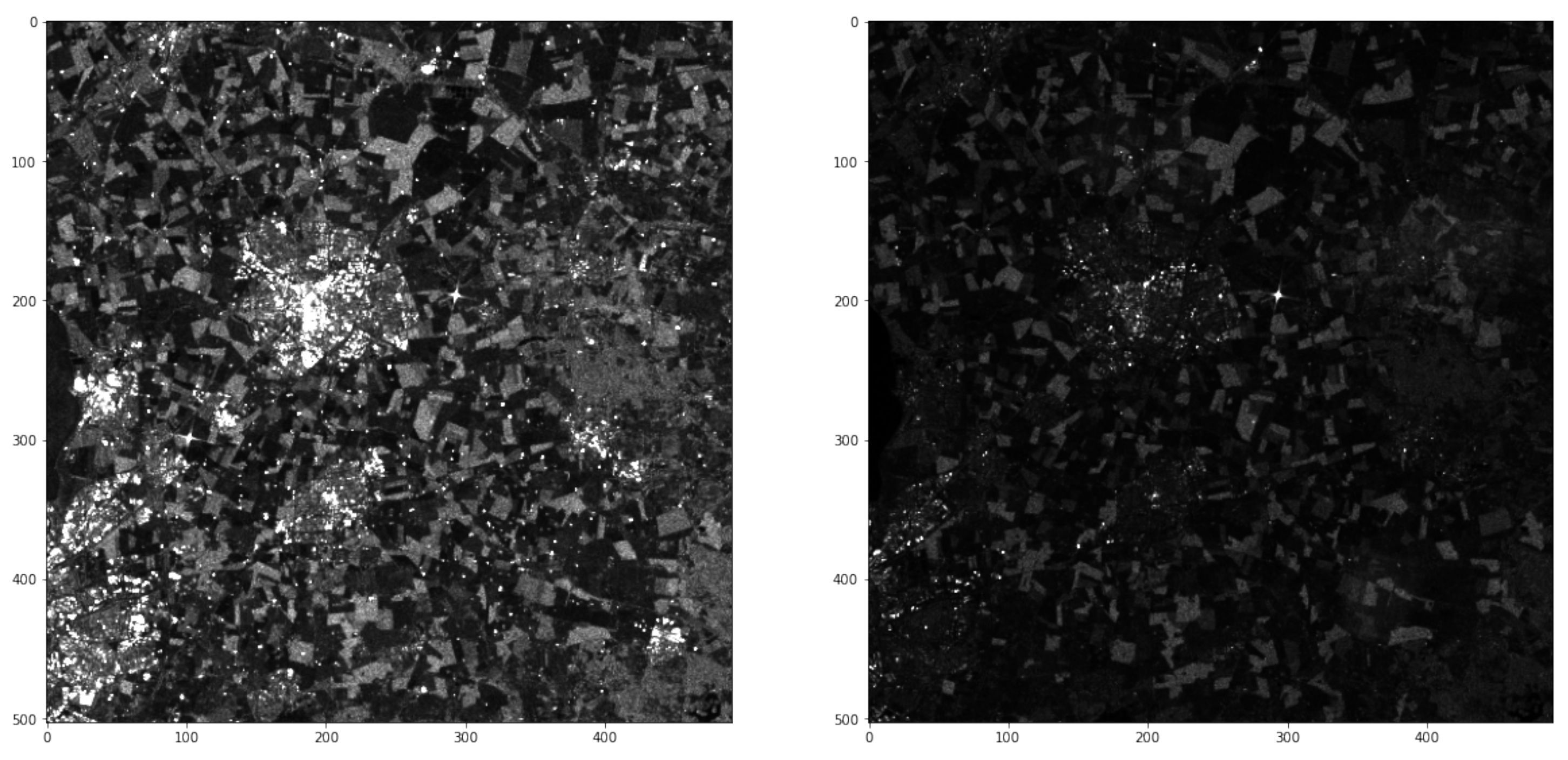
Figure 1.
Typical level-1 SAR backscatter, VH (left), and VV polarization (right), with orthorectification and radiometric calibration.
Figure 1.
Typical level-1 SAR backscatter, VH (left), and VV polarization (right), with orthorectification and radiometric calibration.
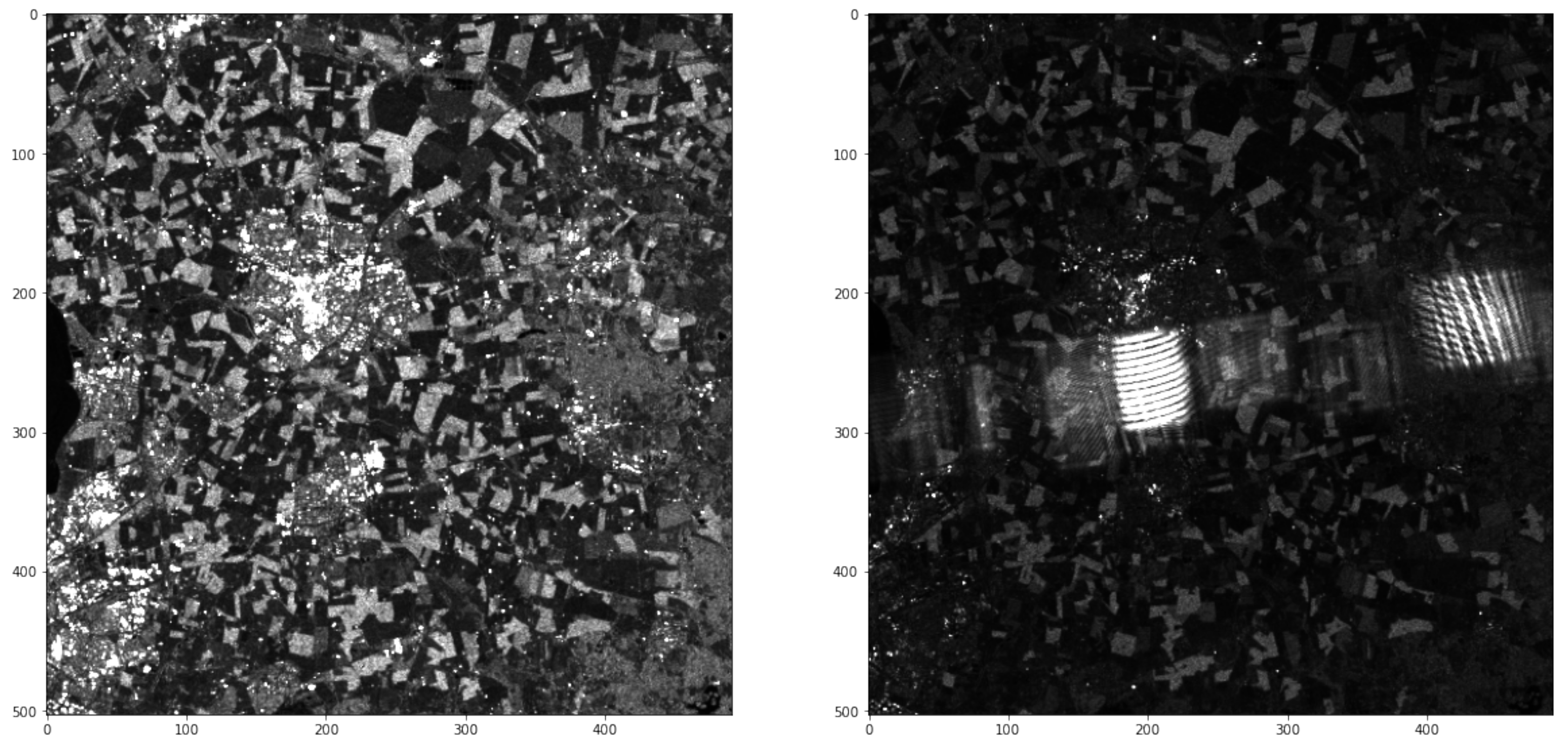
Figure 2.
An example of Sentinel-1 data altered by RFI. VV band (left) is not influenced. VV band (right), however, is heavily affected by RFI.
Figure 2.
An example of Sentinel-1 data altered by RFI. VV band (left) is not influenced. VV band (right), however, is heavily affected by RFI.
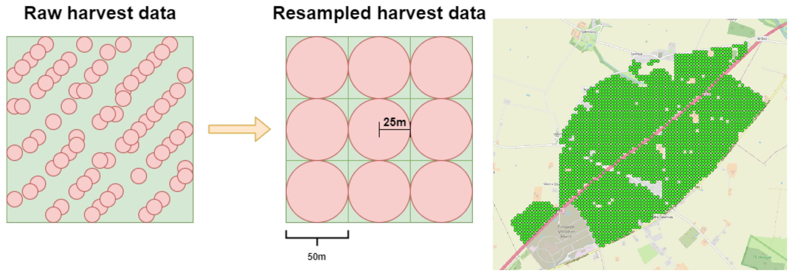
Figure 3.
A geographical overview of the data. The left figure shows the locations of the fields in southwest Sweden. The figure to the right shows the same region where the green tiles represent the regions/patches of Sentinel-1 data downloaded. These patches were selected in order to cover all the fields.
Figure 4.
The Sentinel-1 and weather data were collected from the first of April until the end of July. This end date is approximately a month before harvest, which for winter wheat typically occurs in mid-September in Sweden. In general, however, we only retained a single contribution per week from each of our three input data sources (Sentinel-1, weather, or topography). For Sentinel-1, this was performed by selecting the first RFI-free image from that week. For weather, the daily measurements were accumulated over the whole week.
Figure 5.
Images for VV and VH polarizations before and after applying the transformation and despeckling. The process may have caused some loss of sharpness, but it is generally a significant improvement compared to more traditional speckle filtering techniques [
9].
Figure 5.
Images for VV and VH polarizations before and after applying the transformation and despeckling. The process may have caused some loss of sharpness, but it is generally a significant improvement compared to more traditional speckle filtering techniques [
9].
Figure 6.
Illustration of the unevenly distributed points in the raw yield data and how they were resampled into a grid.
Figure 6.
Illustration of the unevenly distributed points in the raw yield data and how they were resampled into a grid.
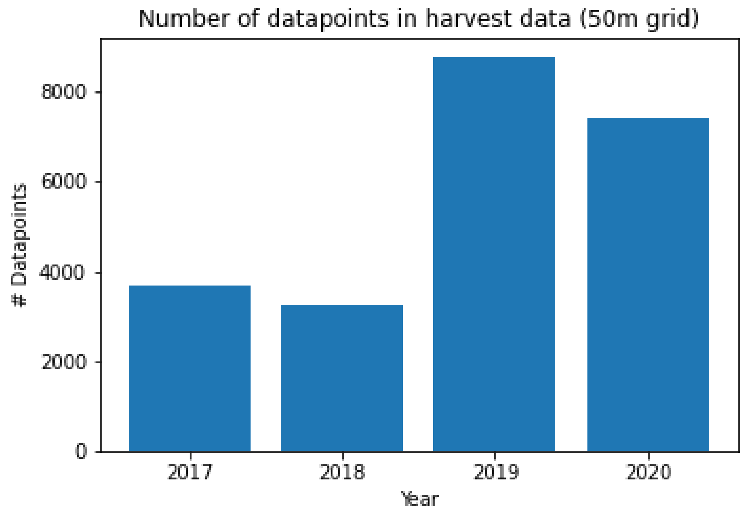
Figure 7.
Winter wheat yield data available for training for each of the study years under the chosen grid. The number of fields where the above data were obtained during the years 2017, 2018, 2019, and 2020 were 49, 31, 132, and 88, respectively.
Figure 7.
Winter wheat yield data available for training for each of the study years under the chosen grid. The number of fields where the above data were obtained during the years 2017, 2018, 2019, and 2020 were 49, 31, 132, and 88, respectively.
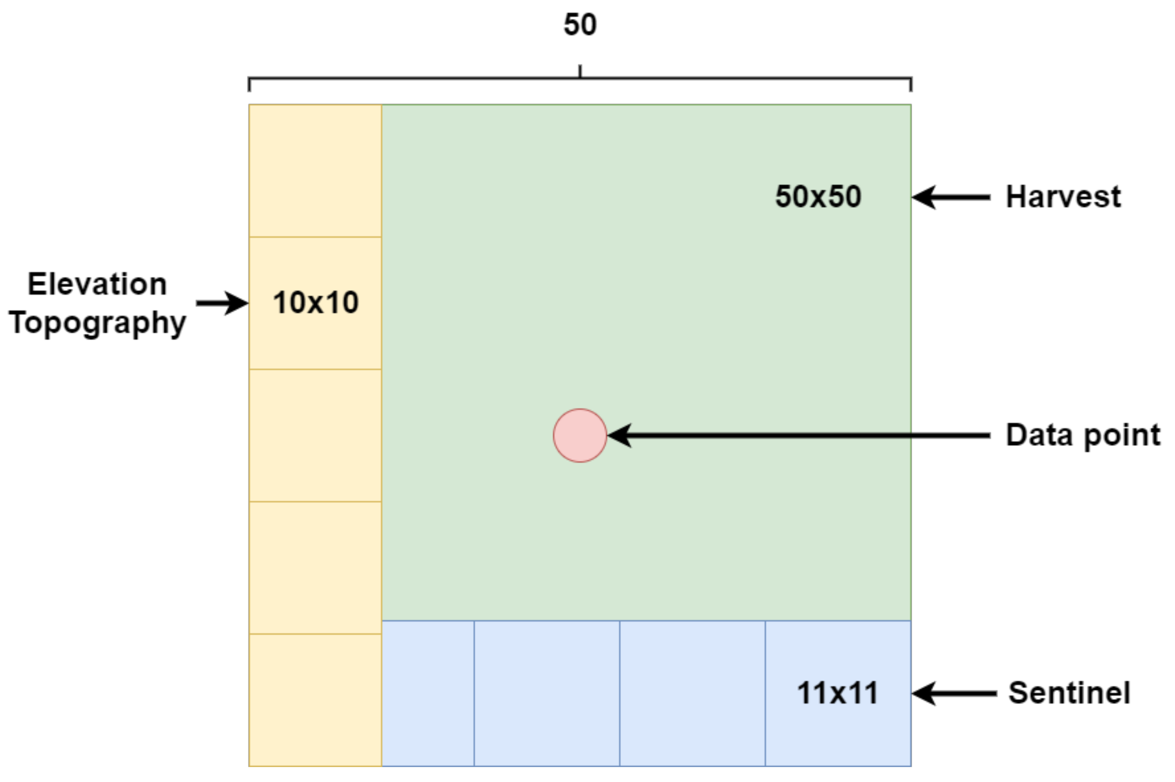
Figure 8.
Visualization of the mismatch in resolution between the yield, Sentinel-1, topography, and elevation data. The lowest resolution was given by the yield data, where each data point summarizes yield within a 50 × 50 area. The satellite data had a finer resolution of 11 × 11 , while the topography and elevation data shared a resolution of 10 × 10 . This resolution difference was the reason for introducing grid sampling instead of just sampling the nearest data point in space.
Figure 9.
The regression RMSE decreased as the size of the dataset increased, with grid G-50 and input VH-VV from Sentinel-1. This result indicates that the Sentinel-1 data contain valuable information for predicting 2019 yield. Results from LGBM (left) and FNN model (right).
Figure 9.
The regression RMSE decreased as the size of the dataset increased, with grid G-50 and input VH-VV from Sentinel-1. This result indicates that the Sentinel-1 data contain valuable information for predicting 2019 yield. Results from LGBM (left) and FNN model (right).
Figure 10.
The predicted yield distribution for 2017 (left), obtained using an LGBM model with grid G-50 and input “All features”, closely matched the true yield distribution (right). The model accurately captured the shape, mean, and variance of the true distribution for this year.
Figure 10.
The predicted yield distribution for 2017 (left), obtained using an LGBM model with grid G-50 and input “All features”, closely matched the true yield distribution (right). The model accurately captured the shape, mean, and variance of the true distribution for this year.
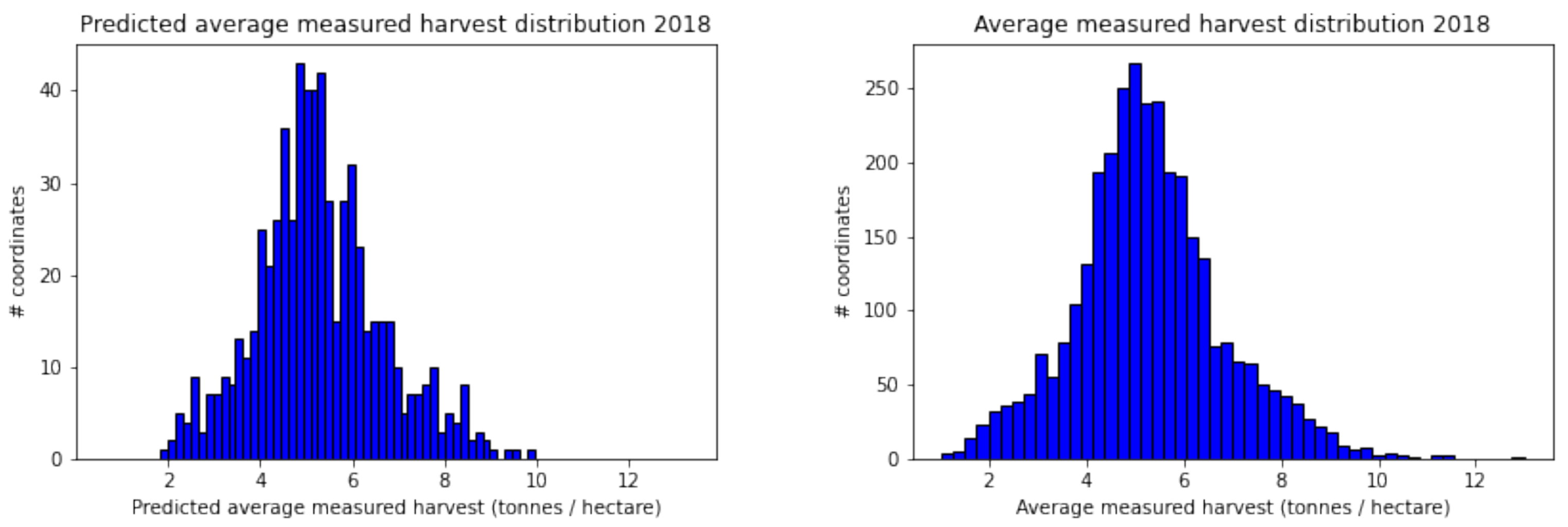
Figure 11.
The predicted yield distribution for 2018 (left), obtained using an LGBM model with grid G-50 and input “All features”, closely matched the true yield distribution (right). The model accurately captured the shape, mean, and variance of the true distribution for this year.
Figure 11.
The predicted yield distribution for 2018 (left), obtained using an LGBM model with grid G-50 and input “All features”, closely matched the true yield distribution (right). The model accurately captured the shape, mean, and variance of the true distribution for this year.
Figure 12.
The predicted yield distribution for 2019 (left), obtained using an LGBM model with grid G-50 and input “All features”, closely matched the true yield distribution (right). The model accurately captured the shape, mean, and variance of the true distribution for this year.
Figure 12.
The predicted yield distribution for 2019 (left), obtained using an LGBM model with grid G-50 and input “All features”, closely matched the true yield distribution (right). The model accurately captured the shape, mean, and variance of the true distribution for this year.
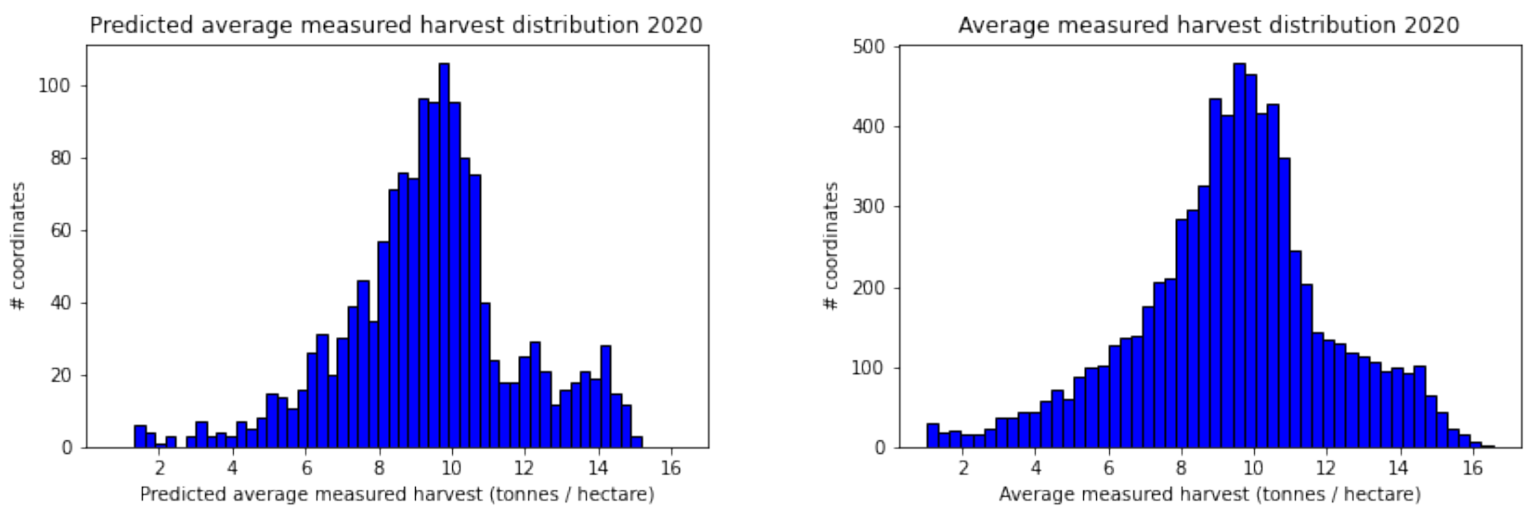
Figure 13.
The predicted yield distribution for 2020 (left), obtained using an LGBM model with grid G-50 and input “All features”, closely matched the true yield distribution (right). The model accurately captured the shape, mean, and variance of the true distribution for this year.
Figure 13.
The predicted yield distribution for 2020 (left), obtained using an LGBM model with grid G-50 and input “All features”, closely matched the true yield distribution (right). The model accurately captured the shape, mean, and variance of the true distribution for this year.
Table 1.
Description of auxiliary training data used.
Table 1.
Description of auxiliary training data used.
| Feature | Description |
|---|
| Weather | Time series of solar irradiance, precipitation, wind speed, temperature, and humidity. |
| Elevation | Single measurement of elevation above sea level at each coordinate. |
| Topographic classification | Topographic terrain classification by Grass GIS geomorphon algorithm encoded with one hot encoding. |
Table 2.
List of different features used in this study and their sizes. Also, note that a random feature is included as a control to uncover a baseline for comparisons.
Table 2.
List of different features used in this study and their sizes. Also, note that a random feature is included as a control to uncover a baseline for comparisons.
| Feature Type | Description | #Features | #Features |
|---|
| | (Nearest) | (Grid) |
|---|
| VH-VV | Processed and min–max normalized VH and VV bands | 32 | 288 |
| Weather | Weekly accumulated or averaged temperature, solar radiation intensity, precipitation, wind speed, and humidity percentage. | 85 | - |
| Topography | One hot encoded topographical classification of terrain | 10 | 90 |
| Elevation | Min–max normalized elevation above sea level | 1 | 9 |
| Random | Random samples from | 32 | - |
| All | Combining VH-VV, Weather, Topography, and Elevation | 128 | 472 |
Table 3.
RMSE for each year, model, feature vector, sampling method, and resolution. The LGBM model outperforms the FNN model in all cases. There seems to be a slight advantage to using Grid sampling. Note that weather is not presented with the Grid sampling method, since we only sample from one weather station per field.
| | | 2017 | 2018 | 2019 | 2020 |
|---|
| | LGBM | FNN | LGBM | FNN | LGBM | FNN | LGBM | FNN |
|---|
| G-50 | All | 0.80 | 1.09 | 0.75 | 0.87 | 0.93 | 1.07 | 1.08 | 1.37 |
| | VH-VV | 0.85 | 1.12 | 0.81 | 0.87 | 1.01 | 1.15 | 1.20 | 1.47 |
| | Topography | 1.35 | 1.47 | 1.51 | 1.58 | 1.82 | 1.90 | 2.67 | 2.77 |
| | Elevation | 1.23 | 1.33 | 1.26 | 1.36 | 1.68 | 1.85 | 2.45 | 2.70 |
| N-50 | All | 0.81 | 1.05 | 0.76 | 0.87 | 0.93 | 1.13 | 1.09 | 1.37 |
| | VH-VV | 0.86 | 1.12 | 0.81 | 0.88 | 1.04 | 1.12 | 1.25 | 1.53 |
| | Weather | 1.08 | 1.29 | 1.11 | 1.39 | 1.34 | 1.52 | 1.66 | 2.05 |
| | Topography | 1.32 | 1.40 | 1.49 | 1.57 | 1.80 | 1.84 | 2.64 | 2.67 |
| | Elevation | 1.24 | 1.33 | 1.29 | 1.35 | 1.75 | 1.83 | 2.54 | 2.68 |
Table 4.
Classification accuracy and F-1 score based on varying error tolerance, in tons/hectare, based on the LGBM model trained with G-50 and All features. Note that the performance increases significantly between .
Table 4.
Classification accuracy and F-1 score based on varying error tolerance, in tons/hectare, based on the LGBM model trained with G-50 and All features. Note that the performance increases significantly between .
| | 2017 | 2018 | 2019 | 2020 |
|---|
| Acc. | F-1 | Acc. | F-1 | Acc. | F-1 | Acc. | F-1 |
|---|
| 0.50 | 0.56 | 0.55 | 0.60 | 0.59 | 0.50 | 0.50 | 0.44 | 0.44 |
| 0.75 | 0.72 | 0.71 | 0.76 | 0.76 | 0.67 | 0.67 | 0.60 | 0.60 |
| 1.00 | 0.83 | 0.82 | 0.86 | 0.86 | 0.79 | 0.78 | 0.72 | 0.72 |
| 1.25 | 0.90 | 0.89 | 0.91 | 0.91 | 0.86 | 0.86 | 0.80 | 0.79 |
| 1.50 | 0.94 | 0.93 | 0.95 | 0.94 | 0.91 | 0.91 | 0.86 | 0.86 |

 ,
, 


