Article

Effects of Weather on Sugarcane Aphid Infestation and Movement in Oklahoma

1
Department of Agricultural Economics, Oklahoma State University, Stillwater, OK 74078, USA
2
Division of Business, Northern Oklahoma College, Stillwater, OK 74078, USA
3
USDA-ARS Plant Science Research Laboratory, Stillwater, OK 74075, USA
4
Department of Entomology, Oklahoma State University, Stillwater, OK 74078, USA
*
Authors to whom correspondence should be addressed.
Agriculture 2023, 13(3), 613; https://doi.org/10.3390/agriculture13030613
Submission received: 23 January 2023 / Revised: 26 February 2023 / Accepted: 1 March 2023 / Published: 3 March 2023
(This article belongs to the Special Issue Application of Econometrics in Agricultural Production)

Abstract

:
Sugarcane aphids have caused economic damage on sorghum and other grain production in Oklahoma. When applied in a timely manner, insecticides provide efficient control; however, it is difficult to protect against the unexpected heavy infestations that have appeared frequently since 2016. This article evaluates the effect of spatial and temporal patterns of weather variables on sugarcane infestation airborne movements. Econometric methods identified persistent northwesterly wind patterns that explain aphid movements. Results serve as a base for sugarcane aphid infestation predictions and to assist stakeholders in developing an early warning system for sorghum producers.

1. Introduction

United States grain sorghum (Sorghum bicolor ssp. bicolor) production maintains a global importance, though it is only regionally important compared to wheat and maize [1]. In 2017, 80% of the world’s total grain sorghum exports originated from North America [2]. Exports to sub-Saharan Africa provide a valuable food source and assist in closing gaps necessary for many developing nations to achieve food security. Elsewhere, sorghum is used as an animal feed in beef and poultry production and on household tables as a sweetener. The total value of grain sorghum produced in the United States (US) in 2019 was USD 151 million, with acreage primarily located in the Great Plains states of Oklahoma, Texas, Kansas, and Nebraska [3,4]. Sorghum is a niche crop for producers in the Great Plains, where its drought tolerance provides an advantage over wheat and maize [5].
Sugarcane aphids (SCA) Melanaphis sacchari (Zehntner) (Hemiptera: Aphididae) were first discovered on US grain sorghum plants during the 2013 growing season and created immediate concerns [6]. Over the following years, SCA have caused subsequent economic damage to sorghum production in Oklahoma, Kansas, Texas, and surrounding states. SCA feeding causes wilting, leaf death, and stunted plant growth, and infestations often result in significant yield loss and economic damage [7]. In extreme cases, SCA can kill grain sorghum plants, though overall damage depends on the period of plant growth stage in which infestation takes hold [7]. Failing to control SCA may result in yield losses of 20–100%, depending on the pest control management practices of the producer [8]. When applied in a timely manner, insecticides provide effective control, making early detection and scouting an important component of pest management.
Studies on the movement of insect damage have been extensively carried out on several crops and regions [9,10,11,12]. Remote sensing (RS) and similar sensor-based methods have been a recent focus of research, with efforts to estimate pest damage and subsequent production losses across broader scales than those confined to the field level [13,14,15,16]. Ye, S. and Rogan, J. proposed an RS method that includes information on changes in forest conditions from mapping early-stage mortality rates caused by bark beetles in Colorado [13]. Magstadt, S. and Gwenzi, D. proposed a similar RS method for the early detection of peeling through mapping spatial patterns of commercial redwood wooden stands [15]. Leal-Sáenz, A. and Waring K. investigated insect damage to Pinus strobiformis in northern Mexico [17]. Gutiérrez, J. and Barry-Ryan C. measured the effects of herbicides on sunflower crops using aerial images of seasonal phases [14]. Other studies measured the effects of mountain pine beetles on tree mortality as explained by environmental variables [16,18,19].
A common conclusion of these studies is that environmental variables affect insect damage on host plant species and that spatial data provide valuable information for mapping and georeferencing insect damage. In particular, the studies emphasize the contribution of various spatial information data sources including moisture indices, Aperture Optical Sciences (AOS), satellite remote sensing data, helicopter-GPS, and aerial photography in providing the required data for spatial analysis. This includes environmental variables that enable synthesizing the biodynamics of organism populations, essential for assessing the temporal and spatial patterns of insect movement. Adding the temporal dimension is consistent with the literature. Robertson, C. and Mulder, M. argue that adding temporal trends in the prediction of spatial patterns improves the predictive ability of insect infestations.
Studies developing spatial and temporal patterns of weather, including their effect on crop yields, have been applied in many fields [20,21] and greatly outnumber studies forecasting patterns of insect movements. Prior studies have often identified persistence in weather patterns, suggesting that pest movements that largely depend on weather can be predicted within statistically significant confidence intervals [22,23]. In the entomological literature, insect movements have primarily been modeled using simulated weather patterns rather than observed weather [24,25]. Simulation methods are acceptable for research, but providing real-time forecasts that have practical use requires the use of actual weather data from recent years.
EDDMapS is a national mapping system that tracks invasive species (insects, wildlife, plants, and disease) and assists producers in near real-time monitoring and control of pests such as SCA. Producers and other stakeholders voluntarily upload infestation reports to the EDDMapS web database. Maps are made available to provide producers with up-to-date information on the spread of ongoing infestations. Such reporting also provides the research community with data that can be used to estimate and create ground-truth models of pest movement, including the effect of weather and other environmental variables on pest population dynamics and migratory movements. Forecasts of the spatial and temporal patterns of pest movements can be integrated with existing platforms such as EDDMapS to provide producers with an early warning system that can alert them to highly probable infestations. Such early warning alarms reinforce the need for scouting and provide additional planning time to enact optimal pest control measures.
The purpose of this study is to determine the effects of spatial and temporal patterns of weather variables on SCA population dynamics and migration. Models based on observed weather data fill a gap in applied entomologic research because they provide improved and more realistic forecasts compared to existing models based on simulated weather. This paper first develops an empirical model of SCA survival and migration based on actual weather data. The weather variables used in the SCA model are evaluated next with a spatial–temporal regression to gauge the effect of weather persistence on migration. The regression model is constructed based on SCA data and is used to explore in-sample model forecasting accuracy. The modeling framework serves as a basis for predicting SCA infestation and, subsequently, producing plans for managing SCA.

2. Methods and Data

2.1. Structural Model of SCA Movement

To measure the effect of weather variables on the probability of predicted migration of SCA, a structural model was developed based on an integrated set of survival and migratory-flight functions. The model uses a daily time step to predict the likely movement of SCA, starting from an initial infestation [24]. Each day, the model updates the survival of the SCA population based on two weather-based probability functions, with one accounting for the effect of rainfall and the other temperature. Wind-related equations then forecast likely SCA flight paths based on prevailing wind speed and its direction. The following subsections describe each of the models’ structural equations, quantifying daily survivability and movement.

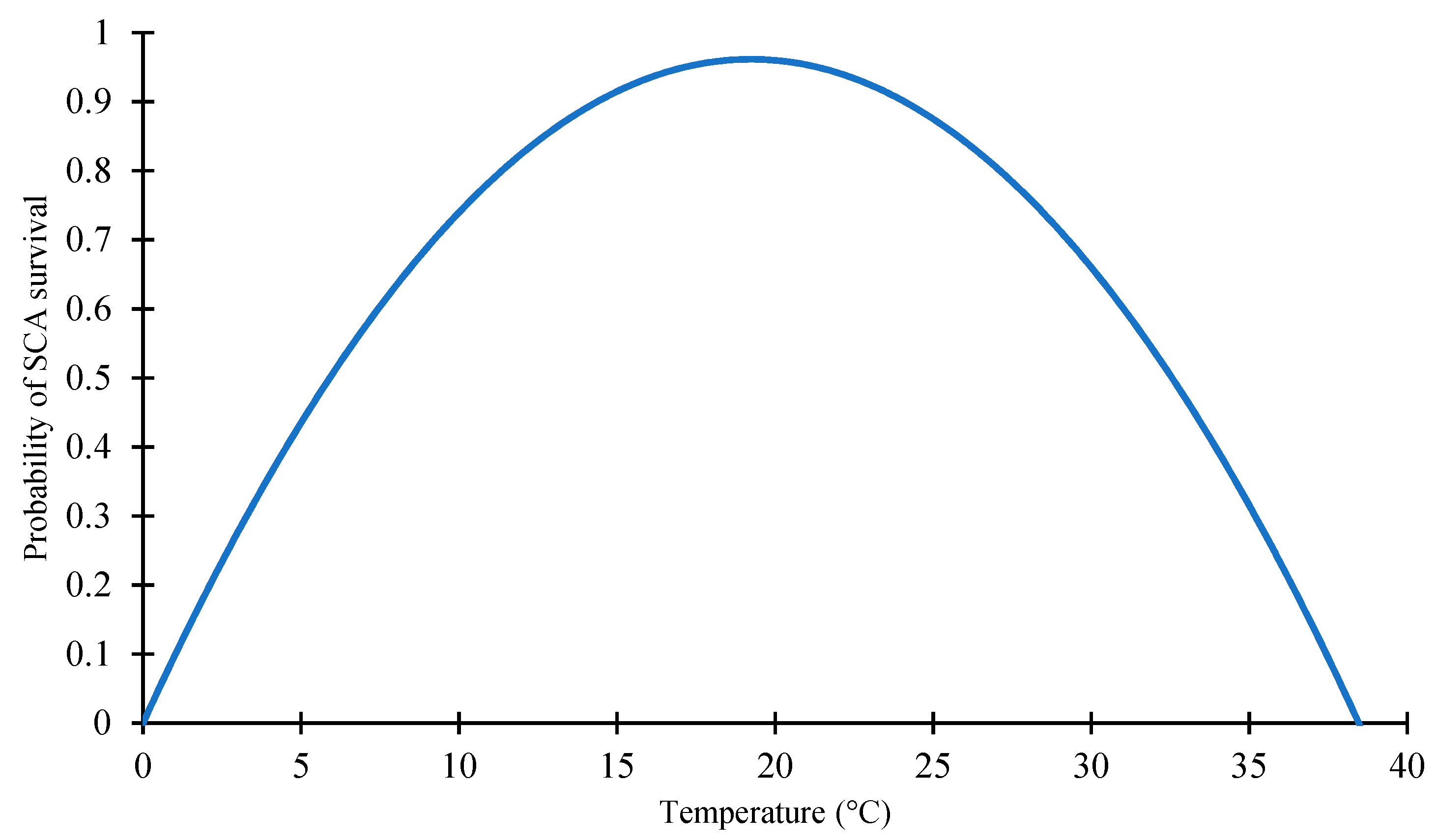
2.1.1. Effect of Temperature on SCA Survivability

Numerous studies report the effect of temperature on the reproduction and survival of SCA, as well as other aphids of similar size and biological features [9,26,27,28,29,30,31,32,33]. In general, although these studies find a diverse and unique response to temperature depending on factors, primarily host plant, they all report temperature’s significant effect on the survival, fecundity, growth, and other transformational properties of aphids. Angleitta, M. and Dunham, A. summarize an even larger number of studies and report that in 73 out of 89 cases, temperature had a positive effect on species growth across temperatures ranging up to 23 °C, beyond which growth turned negative. DeSouza, M. and Armstrong, J. derived SCA survivability and fecundity hosted by sorghum plants in Matagoradoa, TX, a region with agroecological conditions most similar to our Oklahoma study area [33]. Acreman, S.J. and Dixon, A.F. report a similar effect of temperature on the survivability and fecundity of wheat aphids (Sitobion avenae F.).
The daily survivability probability function was developed based on the general characteristics from the prior studies that suggest a quadratic polynomial functional form:
P T A V G = f T A V G = κ T A V G + λ T A V G 2
where P t e m p is the probability of survival, T A V G is the daily average temperature, and κ and λ are parameters affecting the relationship between temperature and SCA survivability ( κ > 0, λ < 0). The quadratic was parametrized to achieve maximum survivability at 20 °C, a compromise between the DeSouza M. and Acreman, S.J. models, corresponding to κ = 0.1 and λ = −0.0026 (Figure 1).

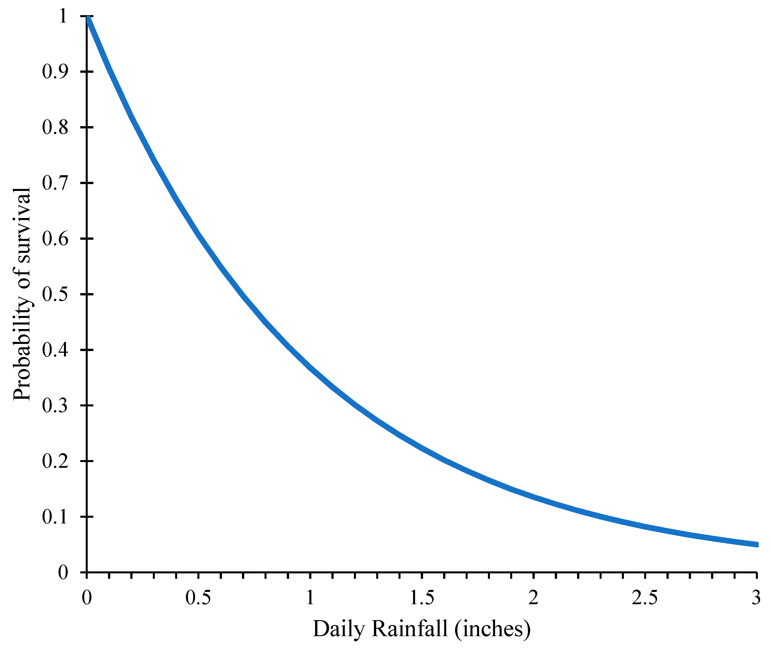
2.1.2. Effect of Rainfall on SCA Survivability

Several experiment station studies have investigated the effect of rainfall on insect survivability. These studies generally report a negative effect on the survival rate and colonization of insects such as SCA [9,10,11,12,34]. Intense rainfall dislodges insects and larvae from the host plant and disrupts feeding and development processes, leading to increased mortality, delayed development, and hindered movement, including flying [10,34,35]. Rainfall’s effect varies by host species and rainfall intensity. Koboro, Y. and Amano, H. report the effect of artificial rainfall intensity as measured by droplet size, which had a significant effect on diamondback moths (Plutella xylostella) hosting on cabbage with larger-sized droplets (3 mm diam.), causing more than 120% more larvae mortality compared to normal droplets (1.7 mm diam.). The survivability of Lepidoptera (Plutella xylostella) feeding on black mustard (Brassica nigra) declined by 36% and 64% when exposed to artificial rainfall of normal and high intensity [10]. In a Bavarian study of Aphidius roseae, foraging on rose bush hosts, survivability, fecundity, foraging, and movement were estimated as explicit functions of discrete rainfall events [34]. Colony survivability decreased by an average of 62.9%, fecundity by 89.4%, foraging by 90.2%, and within-field movement by 35.0% as a result of intense June rainfall. Rainfall’s effect on SCA hosted by sorghum, Sorghum bicolor (L.) Moench, was investigated in Río Bravo, Tamaulipas, Mexico, by Rodriguez-Bosque and Silva under both natural and artificial rainfall events [35]. Their findings are consistent with prior studies that rainfall’s effect is modest at low and normal intensity levels, but increases dramatically under heavy rainfall [36,37,38].
Based on Rodriguez-Bosque, M. and Silva, M., the most relevant to our Oklahoma SCA–sorghum-based study, the daily probability survivability function for rainfall was chosen as:
P r a i n = f R A I N = exp β R A I N
where R is the daily rainfall, β = 3, and exp is the exponential function (Figure 2).

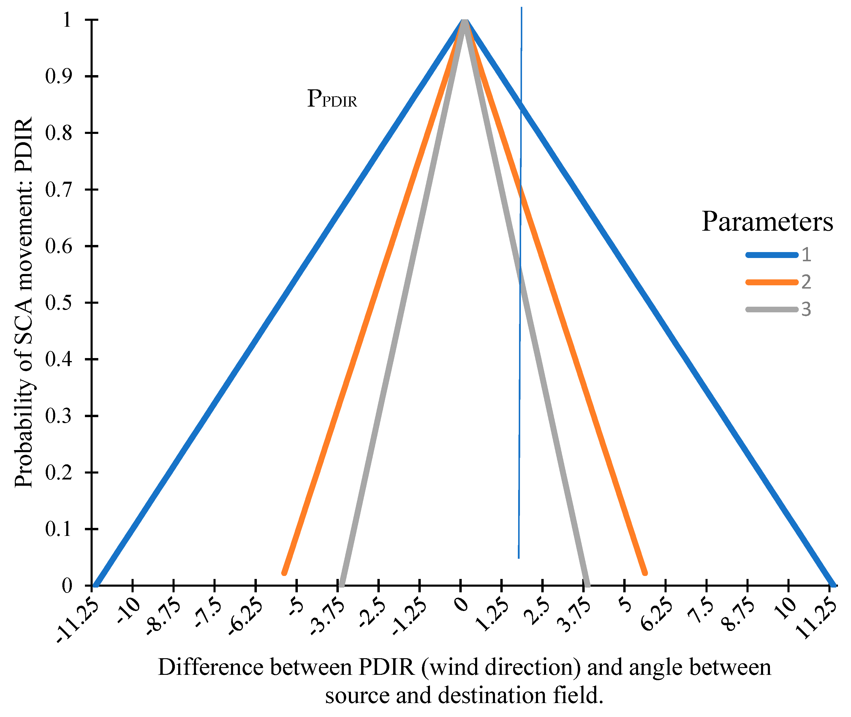
2.1.3. Effect of Wind on SCA Movement

Several studies have dealt with the effects of wind strength, i.e., speed, on the migratory flight patterns of small airborne insect movements such as SCA [35,39,40]. These studies find that wind speed directly affects small organisms such as aphids and is the most important factor in determining the distances that insects travel. Small-sized insects such as SCA essentially “fly with the wind”, as they do not possess adequate strength to change direction or accelerate with or against prevailing wind currents to alter their flight trajectory. Higher wind speeds, hence, increase the expected distances that SCA travel. Existing evidence on the duration of SCA migratory flights is scant, but a reasonable estimate is that SCA travel five hours per day on average. Based on this expected travel time, the probability of distance traveled using the wind speed of the county is given by the following triangular distribution:
P W S P D = f W S P D = 1 W P S D t 5 5 W P S D
where P W S P D is the probability of movement using W S P D , W S P D is the average of all 5 min wind speed observations each day (miles per hours), w is wind speed, and t is the time the SCA travel per day. The probability according to the travel distance according to WSPD is shown in Figure 3 below. Equation (3) shows that the SCA is most likely to travel 5 h according to the wind speed, and the probability decreases as it moves away from it. This means that as the distance between the initial location and the field is closer to the distance traveled for five hours at the corresponding wind speed, the probability that the SCA will move to the field increases. The distance traveled to each field was calculated using the Haversian formula, which was necessary since Euclidean measures are not accurate, given Earth’s curvature. Using the latitude and longitude coordinates of field centroids, the distance between two fields is given by:
d h = 2 a r c c s i n sin 2 θ 2 θ 2 2 + cos θ 1 cos θ 2 sin 2 δ 2 δ 2 2
where θ 2 ,   θ 2 are the field centroid latitudes in radians and δ 2 ,   δ 1 are the field longitude centroids in radians.
There are no studies estimating the correlation between the wind direction and SCA, but studies on observed SCA migratory patterns suggest that wind direction largely determines the vector of SCA movement [35,39,40]. Based on this empirical evidence, a probabilistic function was developed to quantify the likelihood of SCA migration. The function requires the location of both the source field, where SCA infestation has already occurred, and a destination field where migration may occur. If wind direction, as measured from the source field, is in the same direction as the destination field, then the probability of the SCA flying over the destination field is 1, assuming that wind velocity was sufficiently strong (Equation (3)) for the SCA migratory cohort to reach the destination. For wind directions varying away from this ideal situation, the probability of reaching the destination field decreases. The probability distribution has the form of a triangular distribution and is based on the wind direction measurement system used by the Oklahoma Mesonet. This is a 16-point cardinal direction that records daily prevailing wind direction using an integer between 0 and 15, PPDIR, with a corresponding angular range of ±11.25° between each of the 16 possible wind directions. The probability function assumes that flight varies from the primary direction by ±1 wind-directional unit, e.g., a primary direction of 7 is assumed to vary between 6 and 8 by ±11.25°. This parametrization places lower limits on the probability distribution, which declines linearly from a probability of 1 along PPDIR to zero at the boundary between PPDIR and its nearest direction. The probability distribution is shown in Figure 4 and is given by the following formula:
P P D I R = 1 d i σ / 11.25
where P P D I R is probability of movement using the primary wind direction, P D I R is most common wind direction for the day, di is the angular difference in degrees between P D I R and angles, and σ is a parameter (σ > 0) that establishes the boundary where probability equals zero. For this study, a value of σ = 1 was chosen so that the zero-probability boundary occurs at P D I R   ± 1 wind-direction value, whereas other values such as σ = 2 or σ = 3 shift the boundary inward (Figure 4).

2.1.4. Joint Probability of SCA Movement

The modeling of SCA movement took place over 10 days in early June, when SCA infestations typically emerge. The small window of time is appropriate, because the aim was to investigate the flight movement of SCA and the persistence of wind patterns, which are hypothesized to be trending primarily northward in early June. Hence, our aim was to develop a model of SCA survival throughout the ten-day period rather than a complete simulation model. The entomology literature contains excellent examples of such highly developed biophysically and morphologically based aphid and insect simulation models [24]. Moreover, our purpose is not to predict actual aphid populations but to provide probabilities of SCA movement from an initial known location to other fields, so actual population at the time of migration is of much less importance. Probabilities reported in the Results section should be interpreted as the relative probability of SCA infestation on one field compared to others.
Simulation began at an initially infested location i at time t where location is georeferenced at the sorghum field’s centroid and t is measured in days. Each day, the probability of SCA infestation at location i transitioned in according to the temperature and rainfall survival probabilities following in the Leslie population growth approach often used in simulation [25,41,42,43,44]:
P t + 1 i = P t i × P t , r a i n i × P t , t e m p i
where P t , r a i n i and P t , t e m p i are calculated from Equations (1) and (2). A cohort of the remaining SCA population migrated through flight according to the following assumptions: (1) population pressure was sufficiently large to induce migration [24]; (2) a sufficient number of alleles were available each day for migratory flight; and (3) to reduce model complexity, daily migratory SCA population was replaced by colony growth so that daily SCA probability of infestation remained constant.
SCA migration was predicted for all possible paths from field i to all other sorghum fields in Oklahoma. The predicted probability of the SCA cohort movement from field i to a particular field j was calculated based on wind speed (Equation (3)) and wind direction (Equation (5)) that are independent of one another:
P t i j = P t , P D I R i j × P t , W S P D i j   for   t   =   1 , 2     N
where P t i j is the daily probability of moving from initial location i to sorghum field j at time t . Equation (7) is calculated on a daily basis for all 1632 sorghum fields that were actively planted during the initial infestation. Following projected flight movements at time t , the J destination fields were updated beginning on the day following their arrival in the same manner as the source fields. Labeling the newly arrived colonies as P t j , the following day’s probability of survival was updated by the temperature and rainfall survival probabilities given by:
P t + 1 j = P t j × P t , r a i n j × P t , t e m p j
The simulation process was repeated for N = 11 days, always beginning from the initial infestation at location i . Subsequent migration from the J destination fields was not considered since the primary objective is to investigate if persistent weather patterns exist across years. Isolating the predicted movement of a single colony was considered sufficient to achieve our research aim. Once completed, the predicted probability of an SCA infestation on each field j was calculated as the 11-day time average over which the migratory flights were calculated.

2.2. Explaining Spatial Patterns of SCA Movements over Time

The probability of SCA flight migration from an initial infestation in Kiowa County, Oklahoma, was regressed using the GPS coordinates of the destination field’s centroid as explanatory variables. Since the survivability and flight movement probabilities are derived from weather variables, our working hypothesis is that persistence in weather variables implies that field-location regression parameters should likewise be significant. Eight years (2013–2020) of simulated SCA migration generated a balanced dataset of 13,056 observations representing flight migration from an initial infestation in Kiowa County to 1632 destination sorghum fields. Since probabilities are defined in the range from 0 to 1, the use of OLS would provide misleading results. A fractal regression model was hence used since it estimates a logistic function that takes on values from 0 to 1. Its general form is the following:
E ( P j , T   | Z ) = e x p Z 1 + e x p Z
where P j , T is the cumulative probability at the end of the simulation period in year T and Z is a vector of regression parameters. The regression equation uses a 2nd-order polynomial with an interaction term for Z as given by:
Z = a + β 1 X i , j + β 2 Y i , j + β 3 X i , j 2 + β 4 Y i , j 2 + β 5 X i , j Y i , j + d T + ε r t
where X i , j and Y i , j are the relative coordinates measured from field i, the location of the initial infestation in Kiowa County, dt are year dummy variables, a is the intercept, and ε r t is an independently and identically distributed error term for sorghum field r on day t with mean zero and variance σ 2 . The X i , j , Y i , j coordinates were obtained from the georeferenced latitude–longitude of each field’s centroid using ARC-MAP software. The model was estimated in Stata software using the fracreg statement. The estimated regression equation is essentially a probability distribution of SCA movement across two-dimensional space.

2.3. Data

Data used for the SCA weather survival and flight movement simulation equations were daily averaged observations data of air temperature (TAVG), rainfall (RAIN), wind speed (WSPD), and primary wind direction (PDIR) as recorded by the Oklahoma Mesonet. This system includes 119 weather stations located in each county, with some larger counties operating multiple stations. In such cases, weather variables were averaged for each county. Mesonet stations measure TAVG and WSPD based on daily averages of temperature and wind speed measured at 5 min intervals. PDIR is reported as the prevailing wind direction for the day based on a discrete 16-point compass heading, i.e., a 22.5° separation between readings.
The SCA model was run for an eleven-day period, 15–25 June, coinciding with the initial SCA infestation in Kiowa County that was observed in 2018. Since this mid-June time frame is the typical time and place when and where SCA first arrive in Oklahoma, the SCA model was run across the same eleven-day window (15–25 June) using weather conditions from seven other years (2013–2017; 2019–2020) to investigate how SCA movement would have occurred across different years. This constructs a set of panel data from which econometrics can test if weather can explain the temporal and spatial patterns of SCA movement. Hence, model results presented in the following section represent field conditions only for 2018, with other years based on observed weather beginning with the same initial infestation in Kiowa County. Average values of weather variables by year are listed in Table 1.
The SCA migration probabilities were calculated for each sorghum-producing field in Oklahoma. The CROPSCAPE-georeferenced dataset was used to identify the entire population of sorghum-producing fields in Oklahoma (Figure 5). The average number of sorghum fields during the analysis period was 1632. Sorghum production in Oklahoma is mainly concentrated to the western portion of the state, with the primary region in the panhandle. The SCA migration probabilities were calculated using the centroid of Kiowa County as the destination coordinates (Figure 5). This location was selected since the first occurrence of SCA has typically been in this location, or neighboring counties, from early to mid-June [45]. Hence, the SCA probabilities were calculated from 15 June to 25 June. The eleven-day period was chosen since infestations typically last for this length of time before they are either be controlled by pesticides or colonies die off through natural causes. Over an eleven-day period, based on reported sightings, SCA movements were typically in the range of 100 miles.
The probability of SCA movement for a single day, beginning from the source of infestation, Kiowa County, is illustrated in Figure 6. Sample calculations are provided for the field of maximum probability of an SCA airborne infestation, P = 0.37, as indicated by the red square (Figure 6). For this day, 15 June 2018, wind direction was PDIR = 8, indicating a due north wind direction. As a result, only fields contained within a 22.5° spoke emanating from the infested field in Kiowa County, oriented in a due north direction, had non-zero probabilities for this simulation day (Figure 6). All fields outside the spoke had zero probability of SCA migration and are not drawn. Based on Equation (4), fields due north of the infested field had the highest probability based on the prevailing wind direction (PDIR = 8). Moving from the middle of the cone to its boundary decreases the probability of SCA landing on fields in that region. The sample field is oriented −0.19° W of the source field, resulting in a directional probability of PPDIR = 0.983. The effect of wind speed is also evident as the highest probabilities are near the midway point between the infested field and fields furthest to the north. For the sample field, located 91.1 miles from the source field, on a day with a wind speed of 17.9 mph, resulted in a 5.08 h flight. This is extremely close to the ideal 5 h flight, the highest-probability flight time in Equation (3), generating a wind-speed probability of PWSD = 0.9775. SCA colonies successfully landing on a destination field were then updated according to daily rainfall and temperature. The sample field with 0.1766 in of rain and a temperature of 30.1 °C resulted in losses of PRAIN = 0.588 and PTEMP = 0.649 using Equations (1) and (2). Using Equation (7), the overall probability of an SCA colony on the red field was P = 0.37.

3. Results

This section presents the results of the fractal regression model and a discussion of their implications and findings compared to prior research. This includes an assessment of the limitations in our current modeling approach, as well as its potential use in an early warning system.

3.1. Effect of Weather Variables on Predicted Cumulative Probability

The fractal regression model fit the predicted SCA probabilities modestly well with a pseudo R2 of 0.30 and a highly significant Wald test of 1102.13 (Table 2). All of the model parameters were significant at the 5% level or greater except for the year 2014 dummy variable (Table 2). The effect of each regression coefficient on SCA movement was consistent with expectations, as illustrated in Figure 7. For example, ignoring second-order terms, the northwesterly movement found in each year of the simulation is explained by the negative sign on the X variable (westward movement) and the positive sign on the Y variable (northerly movement).
The spatial regression model’s in-sample predictions were reasonably accurate, consistent with the pseudo R2 that explained roughly one third of the model variance (Table 2). Figure 7 illustrates three years of SCA movement: red subfigures represent simulated movements from the SCA model, whereas green subfigures are predicted movements from the regression model. Colored dots represent sorghum fields where output from either the fracreg regression model or the SCA simulated model was greater than 0.5, the threshold value used when interpreting binary variables. Results indicate that the fracreg regression model is able to predict the overall trend in SCA movement across years, which with an average PDIR = 7.42 over the eight years of simulation corresponds to a north-to-northwesterly movement towards the Oklahoma panhandle. Variations in wind patterns across years, in both speed and direction, were not entirely explained by the fracreg regression model (Figure 7). For example, in 2014, there were unusually strong winds to the northeast that were not well-captured by the fractal regression model (Figure 7). Conditions in 2018, when temperature and rainfall events were unusually strong and resulted in fewer forecasted infestations, were also difficult for the regression model to accurately predict (Figure 7).
Marginal effects were significant (5%) for the Y variable and several of the year dummy variables (Table 3). This is likely explained by the strong northerly movement of SCA that is primarily measured by distances along the Y rather than X axis (Table 3). The marginal effect for Y can be interpreted as the increase in probability of SCA infestation for a field located a distance Y miles from the infestation location, i.e., the centroid of Kiowa County. For a typical daily travel distance of 100 miles, the marginal effects indicate that the change in infestation would be 0.00185, according to Table 3. The marginal effects also indicate that weather in 2018 and 2020 had positive, significant effects on SCA infestation, according to the regression model. In 2018, the year effect was greatest, with a marginal effect of 0.002551. When compared to other years, probabilities were, ceteris paribus, forecasted to be as much as 0.004231 larger than in 2016 (Table 3).
The strong level of consistency in predicted pest movements across years, as illustrated in Figure 7, implies the presence of autocorrelation in the weather variables. Statistical tests were thus conducted to identify the presence of spatial, temporal, and joint spatial–temporal correlation. Spatial autocorrelation was identified in all four of the weather variables by both the BSJK and Pesaran tests (Table 4). This supports the working hypothesis that spatially persistent weather patterns existed during the eight-year, eight-day analysis period, and corresponding spatial clustering patterns can be identified. Likewise, the tests identified highly significant (p < 0.05) temporal autocorrelation in all four weather variables except PDIR, which was not significant in the BSJK test (Table 4). A third test found highly significant joint autocorrelation in all four weather variables, implying persistent weather patterns across both time and space.

3.2. Discussion

Prior research has developed numerous simulation models that, in general, include processes for population growth, instar development, reproduction, allele, flight dispersal, and survivability [24,25,45,46]. Our flight dispersal–survivability-based simulation is most similar to Kowalweski, T. and Wang, H., who developed an SCA flight dispersal model for Oklahoma and two bordering states, Texas and Kansas, with initial infestations in the Rio Bravo Valley in south Texas [45]. Their simulation utilizes simulated weather data and an atmospheric dispersal model (NOAA-HYSPLIT) that predicted SCA flight movement among 25 × 25 km sized grids, a much coarser scale than the field level used in this paper. Their primary method of model validation was comparisons between observed and simulated dates of the first SCA infestations reported between 2015 and 2019 as part of the EDDMapS database. For Oklahoma, their simulation was able to predict the average date of first SCA arrival within 7 days, to within 1 day of the latest first arrival, and to within 51 days of the earliest first arrival [45]. Using Passing-Bablok regressions on predicted versus actual days to first infestation, no significant difference was found between them in Texas and Oklahoma, suggesting the simulation model performed well in predicting regional SCA movements, though the Kansas prediction was significantly different from observed outbreaks.
Our model provides complementary and more detailed, localized predictions of subsequent movements following an initial infestation that prior research has not addressed. Though too limited in scope at this point for a formal validation, Figure 8 illustrates the probability of SCA movement at the end of our simulation in June and the location of two EDDMapS-reported SCA infestations, one in Caddo County (20 June 2018) and another in Grady County (21 June 2018). Although the two observed outbreaks were not accurately predicted by our model, our model identified a single hotspot in Ellis County, 110 miles northwest of the initial infestation, which is consistent with overall pest movement during this time of year. While the Caddo and Grady County infestations could have been caused by other fields with unreported infestations, misspecified components of our current model are an equally likely source of error.
One of the most critical features that our future research will address is to use a more complete modeling of wind currents that carry SCA through their flight. We currently use ground-based wind trajectories that are only accurate for flights up to approximately 100 feet, but atmospheric wind currents change in speed and direction at altitudes above this height. This would be the most likely explanation for the lack of model validation shown in Figure 7, since the prevailing ground wind was in the northwest direction with only one day when wind direction was favorable to Caddo and Grady Counties. It is likely that upper-level wind currents were more random and included both due easterly and westerly directions that would explain infestations in Caddo and Greer Counties (Figure 8). Future modeling needs to consider a multilayered approach to SCA flight, considering altitudes up to 10,000 feet.
Flight time is also a critical parameter when predicting dispersal. Kowalweski, T. and Wang, H. consider a longer range of flight time in their modeling work, with a range between 12 and 15 h. Our model considers a range of flight time between 0 and 10 h, with the highest probability at 5 h. Future modeling needs to consider incorporating longer flight times as well.

3.3. Population Survivability

The survivability functions could also create difficulties in obtaining a significant model validation. Our temperature survivability function was based primarily on DeSouza, M. and Armstrong, J., who derived SCA survivability (and fecundity) hosted by sorghum plants in Matagoradoa, TX, a region with agroecological conditions most similar to our Oklahoma study area [33]. Field trials were conducted using growth chambers across a controlled range of temperatures from 5 to 35 °C in 5 °C increments. SCA survivability increased from an expected lifespan of 8.8 days at 5 °C to a maximum life of 47.4 days at 15 °C. Survivability decreased for the remaining hotter temperatures, falling to an expected 8.7-day survivability at 35 °C. SCA fecundity was more temperature-sensitive as the extreme temperatures of 5 °C and 35 °C prevented reproduction and only 0.1 nymphs per day were produced at 10 °C. Fecundity then increased more rapidly, reaching a maximum of 2.4 nymphs per day at 30 °C.
Acreman, S.J. and Dixon, A.F. also reported a similar effect of temperature on the survivability and fecundity of wheat aphids [26] (Sitobion avenae F.). Following a similar experimental design to DeSouza, M. and Armstrong, J., they also reported a maximum wheat aphid survivability of 8.3 days at 15 °C and a maximum fecundity of 3.9 nymphs per day at 25 °C. The resulting curve from Equation (1) is in close proximity to those models. For example, at 15 °C, the models predicted daily mortality probabilities of 97.9% and 92.4%, respectively, while Equation (1) predicts a 91.5% mortality. At 25 °C, the temperature most reflective of conditions observed during our study period, the models predicted daily mortality probabilities of 96.5% and 87.7%, respectively, while Equation (1) predicts an 85.5% mortality. Since our current model did not perform well in a limited validation exercise, future modeling will need to consider additional survival functions to improve validation.
The effect of rainfall on survivability is more difficult to assess due to differences in the data available for our study and those used in previous studies. Weather observations available to this study unfortunately did not include rainfall intensity, e.g., hourly rainfall, which previous studies concluded had a more significant effect than total rainfall. Population losses due to rainfall, modeled in Equation (2), should be modified in future research to include a more refined equation that accounts for rain intensity through hourly or even shorter-duration rainfall measurements (Figure 2). This is particularly important since late spring and summer rainfall in Oklahoma is typically intense, and the daily rainfall used in this study is likely an aggregate of several storms, each high in intensity and of short duration. For example, 1 in (25.4 mm) of daily rainfall could likely be two storm events of 15 min with an intensity of 50.8 mm per hr of rainfall. Our current model would underpredict SCA population losses from rainfall. For example, our model predicts a loss of 63.2% compared to the 78.0% loss predicted by Rodriguez-Bosque under actual rainfall conditions.

3.4. Weather Persistence and Improved Forecasting

The significant explanatory power of the spatial regression model provides empirical support that persistent wind patterns existed during the study period that are further corroborated by the spatial and temporal autocorrelation reported in Table 4. This is a meaningful finding since known weather patterns should result in more accurate predictions and are expected to provide localized models such as ours an advantage over regional models that rely on simulated data that have no forecasting capacity. Hence, approaches such as the one presented in this paper are better suited for an early warning system. Existing extension networks have integrated a large number of producers into various information-sharing programs including pest management. State reporting of infestations typically occurs from county-level agents scouting alongside producers. Once identified, state agencies relay this information to producers through web-based portals, providing recommended treatments and maps indicating affected farms. Recent advances in AI and image detection are on the verge of adoption and are expected to vastly improve scouting by reducing time in the field, and improve accuracy.
To function as an early warning system, existing reporting methods need to provide producers with forecasted movements in real-time so farms can be adequately prepared for upcoming events. The preliminary findings in this paper suggest that the joint spatial–temporal autocorrelation identified in the weather panel data could be the basis of a pest movement-forecasting tool for airborne infestations that are highly dependent on prevailing wind currents, such as SCA. Once identified, infested-field location could be used to initiate the forecasting procedure by combining predicted weather outcomes based on both previous years, through the temporal autocorrelation, and across the statewide farming community through spatial autocorrelation. Temporal autocorrelation would provide a weather forecast based on a daily time step, using information from previous weather. For example, an infestation reported on 10 June could be forecasted using expected weather on 11 June since the temporal autocorrelation implies prior days’ weather has significant explanatory power. Likewise, the spatial autocorrelation would provide improved forecasts across space. For example, fields in flight proximity of an infested field would have weather forecasts based on their location in regard to the infested field. The spatial autocorrelation implies that having field location provides significant forecasting power. The forecasted weather could then be fed into a daily time step pest movement model, such as that developed in this paper, to provide producers with expected areas of infestation.

4. Conclusions

In this study, the temporal and spatial characteristics of weather variables were investigated to assess whether SCA movements could be forecasted. Spatial and temporal correlations of weather variables were estimated and results suggest that wind direction, wind speed, average temperature, and precipitation have joint spatial and temporal autocorrelation in both cross-sectional data and panel data, exhibiting persistence. While further analysis is required to develop findings across different climatic regions, initial evidence indicates that weather variables could potentially be utilized in forecasting SCA movements.
A critical need is to continue developing early warning programs to provide producers with adequate time to prepare for likely infestations. The scant data available on SCA infestation make it difficult for model validation and calibration. Ongoing efforts that encourage producers to upload their SCA scouting and monitoring findings in real time, in conjunction with AI-based cell phone apps that greatly reduce scouting time, should continue and be expanded as it is unlikely that satellite imagery or related technology will be able to substitute for manually based scouting approaches.
The model presented in this paper was intended primarily to investigate weather patterns and to assess if there was adequate predictive power to provide contemporaneous forecasts of SCA movement. In future research, the equations governing SCA movement need to be expanded to include additional variables and model parameters estimated based on empirical data. Estimation is currently challenged by lack of observed SCA infestations, but over time, data will become increasingly available. This could include the effect of wind, plant growth stage, and plant stress on SCA survivability. The latter could be of particular importance since water-stressed plants are typically more susceptible to phytophagous insects due to increased nitrogen availability [12]. Weather variability and extreme events could also be included in the negative effects of extreme, fluctuating temperatures. Machine learning and similar estimation approaches can be utilized to train the governing equations consistent with observed outbreaks, including the use newly developed algorithms based on deep learning.
Future modeling could include a broader geographic scope and a longer time span encompassing earlier migratory movements. SCA are believed to begin their northward migration in early spring from southern Texas, near latitudes where temperatures remain above freezing. This paper presented a modest framework to forecast movement from a single location over an expected colony lifespan of ten days. While additional scrutiny is warranted, findings suggest that weather persistence could provide significant predictive power. A suggested second-generation modeling approach would consider tracking daily SCA movements from a larger number of infested fields. From experience gained in developing the model presented in this paper, considering simultaneous outbreaks is expected to greatly increase computing requirements. Artificial intelligence algorithms, including machine learning and neural networks, should be explored as possible approaches.

Author Contributions

Conceptualization, J.V. and P.V.; methodology, S.L. and J.V.; software, D.L.; validation, J.V.; formal analysis, P.V., J.V. and D.L.; investigation, N.E. and K.G.; resources, N.E.; writing—original draft preparation, S.L. and D.L.; writing—review and editing, P.V. and J.V.; visualization, N.E. and K.G.; supervision, J.V., D.L. and K.G.; project administration, N.E. and K.G.; funding acquisition, J.V. All authors have read and agreed to the published version of the manuscript.

Funding

The USDA Agricultural Research Service provided funding for this project through the Areawide Pest Management Program Areawide Pest Management of the Invasive Sugarcane Aphid in Grain Sorghum, project number 3072-22000-017-12-S. Mention of trade names or commercial products in this publication is solely for the purpose of providing specific information and does not imply recommendation or endorsement by the U.S. Department of Agriculture. USDA is an equal opportunity provider and employer.

Institutional Review Board Statement

Not applicable.

Informed Consent Statement

Not applicable.

Data Availability Statement

Data is available upon request from contact author.

Conflicts of Interest

The authors declare no conflict of interest.

References

  1. Aruna, C.; Suguna, M.; Visarada, K.; Deepika, C.; Ratnavathi, C.; Tonapi, V. Identification of sorghum genotypes suitable for specific end uses: Semolina recovery and popping. J. Cereal Sci. 2020, 93, 102955. [Google Scholar] [CrossRef]
  2. Foreign Agricultural Service (FAS). Available online: https://www.fas.usda.gov/data (accessed on 28 February 2023).
  3. Brewer, M.J.; Gordy, J.W.; Kerns, D.L.; Woolley, J.B.; Rooney, W.L.; Bowling, R.D. Sugarcane aphid population growth, plant injury, and natural enemies on selected grain sorghum hybrids in Texas and Louisiana. J. Econ. Entomol. 2017, 110, 2109–2118. [Google Scholar] [CrossRef]
  4. Gordy, J.W.; Brewer, M.J.; Bowling, R.D.; Buntin, G.D.; Seiter, N.J.; Kerns, D.L.; Reay-Jones, F.P.; Way, M. Development of economic thresholds for sugarcane aphid (Hemiptera: Aphididae) in susceptible grain sorghum hybrids. J. Econ. Entomol. 2019, 112, 1251–1259. [Google Scholar] [CrossRef] [PubMed]
  5. Bergtold, J.S.; Ramsey, S.; Maddy, L.; Williams, J.R. A review of economic considerations for cover crops as a conservation practice. Renew. Agric. Food Syst. 2017, 34, 62–76. [Google Scholar] [CrossRef]
  6. Smith, C.M.; Chuang, W.P. Plant resistance to aphid feeding: Behavioral, physiological, genetic and molecular cues regulate aphid host selection and feeding. Pest Manag. Sci. 2014, 70, 528–540. [Google Scholar] [CrossRef] [PubMed]
  7. Elliott, N.; Brewer, M.; Seiter, N.; Royer, T.; Bowling, R.; Backoulou, G.; Gordy, J.; Giles, K.; Lindenmayer, J.; McCornack, B. Sugarcane Aphid1 Spatial Distribution in Grain Sorghum Fields. Southwest. Entomol. 2017, 42, 27–35. [Google Scholar] [CrossRef]
  8. Szczepaniec, A. Assessment of a density-based action threshold for suppression of sugarcane aphids,(Hemiptera: Aphididae), in the Southern High Plains. J. Econ. Entomol. 2018, 111, 2201–2207. [Google Scholar]
  9. Ukoroije, R.B.; Otayor, R.A. Review on the bio-insecticidal properties of some plant secondary metabolites: Types, formulations, modes of action, advantages and limitations. Asian J. Res. Zool. 2020, 3, 27–60. [Google Scholar]
  10. Chen, C.; Harvey, J.A.; Biere, A.; Gols, R. Rain downpours affect survival and development of insect herbivores: The specter of climate change? Ecology 2019, 100, e02819. [Google Scholar] [CrossRef] [Green Version]
  11. Kobori, Y.; Amano, H. Effect of rainfall on a population of the diamondback moth, Plutella xylostella (Lepidoptera: Plutellidae). Appl. Entomol. Zool. 2003, 38, 249–253. [Google Scholar] [CrossRef] [Green Version]
  12. Huberty, A.F.; Denno, R.F. Plant water stress and its consequences for herbivorous insects: A new synthesis. Ecology 2004, 85, 1383–1398. [Google Scholar] [CrossRef]
  13. Ye, S.; Rogan, J.; Zhu, Z.; Hawbaker, T.J.; Hart, S.J.; Andrus, R.A.; Meddens, A.J.; Hicke, J.A.; Eastman, J.R.; Kulakowski, D. Detecting subtle change from dense Landsat time series: Case studies of mountain pine beetle and spruce beetle disturbance. Remote Sens. Environ. 2021, 263, 112560. [Google Scholar] [CrossRef]
  14. Gutierrez, J.; Barry-Ryan, C.; Bourke, P. The antimicrobial efficacy of plant essential oil combinations and interactions with food ingredients. Int. J. Food Microbiol. 2008, 124, 91–97. [Google Scholar] [CrossRef] [PubMed] [Green Version]
  15. Magstadt, S.; Gwenzi, D.; Madurapperuma, B. Can a Remote Sensing Approach with Hyperspectral Data Provide Early Detection and Mapping of Spatial Patterns of Black Bear Bark Stripping in Coast Redwoods? Forests 2021, 12, 378. [Google Scholar] [CrossRef]
  16. Meddens, A.J.; Hicke, J.A. Spatial and temporal patterns of Landsat-based detection of tree mortality caused by a mountain pine beetle outbreak in Colorado, USA. For. Ecol. Manag. 2014, 322, 78–88. [Google Scholar] [CrossRef]
  17. Leal-Sáenz, A.; Waring, K.M.; Sniezko, R.A.; Menon, M.; Hernández-Díaz, J.C.; López-Sánchez, C.A.; Martínez-Guerrero, J.H.; Mariscal-Lucero, S.D.R.; Silva-Cardoza, A.; Wehenkel, C. Differences in cone and seed morphology of Pinus strobiformis and Pinus ayacahuite. Southwest. Nat. 2021, 65, 9–18. [Google Scholar] [CrossRef]
  18. Robertson, C.; Wulder, M.; Nelson, T.; White, J. Risk rating for mountain pine beetle infestation of lodgepole pine forests over large areas with ordinal regression modelling. For. Ecol. Manag. 2008, 256, 900–912. [Google Scholar] [CrossRef]
  19. White, J.; Coops, N.; Hilker, T.; Wulder, M.; Carroll, A. Detecting mountain pine beetle red attack damage with EO-1 Hyperion moisture indices. Int. J. Remote Sens. 2007, 28, 2111–2121. [Google Scholar] [CrossRef]
  20. O’Neal, M.R.; Frankenberger, J.R.; Ess, D.R. Use of CERES-Maize to study effect of spatial precipitation variability on yield. Agric. Syst. 2002, 73, 205–225. [Google Scholar] [CrossRef]
  21. Kravchenko, A.; Robertson, G.; Thelen, K.; Harwood, R. Management, topographical, and weather effects on spatial variability of crop grain yields. Agron. J. 2005, 97, 514–523. [Google Scholar] [CrossRef] [Green Version]
  22. Stevens, S.C. Evidence for a Weather Persistence Effect on the Corn, Wheat and Soybean Growing Season Price Dynamics. 1990. Available online: https://ageconsearch.umn.edu/record/13907/ (accessed on 28 February 2023).
  23. Weatherhead, E.; Gearheard, S.; Barry, R.G. Changes in weather persistence: Insight from Inuit knowledge. Glob. Environ. Chang. 2010, 20, 523–528. [Google Scholar] [CrossRef]
  24. Duffy, C.; Fealy, R.; Fealy, R.M. An improved simulation model to describe the temperature-dependent population dynamics of the grain aphid, Sitobion avenae. Ecol. Model. 2017, 354, 140–171. [Google Scholar] [CrossRef] [Green Version]
  25. Ma, Z.S.; Bechinski, E.J. A survival-analysis-based simulation model for Russian wheat aphid population dynamics. Ecol. Model. 2008, 216, 323–332. [Google Scholar] [CrossRef]
  26. Acreman, S.; Dixon, A. The effects of temperature and host quality on the rate of increase of the grain aphid (Sitobion avenae) on wheat. Ann. Appl. Biol. 1989, 115, 3–9. [Google Scholar] [CrossRef]
  27. Angilletta, J.; Michael, J.; Dunham, A.E. The temperature-size rule in ectotherms: Simple evolutionary explanations may not be general. Am. Nat. 2003, 162, 332–342. [Google Scholar] [CrossRef] [Green Version]
  28. Asin, L.; Pons, X. Effect of high temperature on the growth and reproduction of corn aphids (Homoptera: Aphididae) and implications for their population dynamics on the northeastern Iberian peninsula. Environ. Entomol. 2001, 30, 1127–1134. [Google Scholar] [CrossRef]
  29. Auad, A.; Alves, S.; Carvalho, C.; Silva, D.; Resende, T.; Veríssimo, B. The impact of temperature on biological aspects and life table of Rhopalosiphum padi (Hemiptera: Aphididae) fed with signal grass. Fla. Entomol. 2009, 92, 569–577. [Google Scholar] [CrossRef]
  30. Bale, J.S.; Masters, G.J.; Hodkinson, I.D.; Awmack, C.; Bezemer, T.M.; Brown, V.K.; Butterfield, J.; Buse, A.; Coulson, J.C.; Farrar, J. Herbivory in global climate change research: Direct effects of rising temperature on insect herbivores. Glob. Chang. Biol. 2002, 8, 1–16. [Google Scholar] [CrossRef]
  31. Murúa, M.G.; Vera, M.A.; Michel, A.; Casmuz, A.S.; Fatoretto, J.; Gastaminza, G. Performance of field-collected Spodoptera frugiperda (Lepidoptera: Noctuidae) strains exposed to different transgenic and refuge maize hybrids in Argentina. J. Insect Sci. 2019, 19, 21. [Google Scholar] [CrossRef] [Green Version]
  32. Souza, M.; Davis, J. Detailed characterization of Melanaphis sacchari (Hemiptera: Aphididae) feeding behavior on different host plants. Environ. Entomol. 2020, 49, 683–691. [Google Scholar] [CrossRef] [PubMed]
  33. De Souza, M.A.; Armstrong, J.S.; Hoback, W.W.; Mulder, P.G.; Paudyal, S.; Foster, J.E.; Payton, M.E.; Akosa, J. Temperature dependent development of sugarcane aphids Melanaphis Sacchari, (Hemiptera: Aphididae) on three different host plants with estimates of the lower and upper threshold for fecundity. Curr. Trends Entomol. Zool. Stud. 2019. [Google Scholar] [CrossRef]
  34. Weisser, W.W.; Volkl, W.; Hassell, M.P. The importance of adverse weather conditions for behaviour and population ecology of an aphid parasitoid. J. Anim. Ecol. 1997, 1, 386–400. [Google Scholar] [CrossRef]
  35. Rodríguez-del-Bosque, L.A.; Silva-Serna, M.M.; Aranda-Lara, U. Effect of Natural and Simulated Rainfall and Wind on Melanaphis sacchari1 on Sorghum. Southwest. Entomol. 2020, 45, 357–364. [Google Scholar] [CrossRef]
  36. Balikai, R.; Lingappa, S. Bio-Ecology and Management of Sorghum Aphid: Melanaphis Sacchari; LAP LAMBERT Academic Publishing: Saarland, Germany, 2012. [Google Scholar]
  37. Patel, D.; Purohit, M. Influence of different weather parameters on aphid, Melanaphis sacchari infesting Kharif sorghum. Int. J. Plant Prot. 2013, 6, 484–486. [Google Scholar]
  38. Colares, F.; Michaud, J.; Bain, C.L.; Torres, J.B. Indigenous aphid predators show high levels of preadaptation to a novel prey, Melanaphis sacchari (Hemiptera: Aphididae). J. Econ. Entomol. 2015, 108, 2546–2555. [Google Scholar] [CrossRef]
  39. Mann, J.A.; Tatchell, G.M.; Dupuch, M.J.; Harrington, R.; Clark, S.J.; McCartney, H.A. Movement of apterous Sitobion avenae (Homoptera: Aphididae) in response to leaf disturbances caused by wind and rain. Ann. Appl. Biol. 1995, 126, 417–427. [Google Scholar] [CrossRef]
  40. Shao, X.; Zhang, Q.; Liu, Y.; Yang, X. Effects of wind speed on background herbivory of an insect herbivore. Écoscience 2020, 27, 71–76. [Google Scholar] [CrossRef]
  41. Leslie, P.H. On the use of matrices in certain population mathematics. Biometrika 1945, 33, 183–212. [Google Scholar] [CrossRef]
  42. Nordheim, E.V.; Hogg, D.B.; Chen, S.-Y. Leslie matrix models for insect populations with overlapping generations. In Estimation and Analysis of Insect Populations; Springer: Berlin/Heidelberg, Germany, 1989; pp. 289–298. [Google Scholar]
  43. Carter, N.; Aikman, D.; Dixon, A. An appraisal of Hughes’ time-specific life table analysis for determining aphid reproductive and mortality rates. J. Anim. Ecol. 1978, 47, 677–687. [Google Scholar] [CrossRef]
  44. Bannerman, J.A.; Roitberg, B.D. Impact of extreme and fluctuating temperatures on aphid–parasitoid dynamics. Oikos 2014, 123, 89–98. [Google Scholar] [CrossRef]
  45. Koralewski, T.E.; Wang, H.-H.; Grant, W.E.; Brewer, M.J.; Elliott, N.C. Evaluation of Areawide Forecasts of Wind-borne Crop Pests: Sugarcane Aphid (Hemiptera: Aphididae) Infestations of Sorghum in the Great Plains of North America. J. Econ. Entomol. 2022, 115, 863–868. [Google Scholar] [CrossRef] [PubMed]
  46. Wennergren, U.; Landin, J. Population growth and structure in a variable environment: I. Aphids and temperature variation. Oecologia 1993, 93, 394–405. [Google Scholar] [CrossRef] [PubMed]
Figure 1. Relationship between probability of SCA survival and temperature based on Equation (1) (κ = 0.1, λ = −0.0026).
Agriculture 13 00613 g001
Figure 2. Probability of SCA survival as given by rainfall (β = 3).
Agriculture 13 00613 g002
Figure 3. Probability of SCA movement along a straight-line distance from initial infestation to destination field.
Agriculture 13 00613 g003
Figure 4. Probability of SCA migratory flight landing on destination field as a function of angular deviation from daily observed wind direction.
Agriculture 13 00613 g004
Figure 5. Georeferenced map of sorghum fields in Oklahoma identified during the 2018 growing season. Source: CROPSCAPE.
Agriculture 13 00613 g005
Figure 6. SCA flight migration on day 1 of simulation, 15 June 2018, showing the probability of movement from initial infestation to destination fields. Source: Authors’ calculations.
Agriculture 13 00613 g006
Figure 7. Regression predicted (green) and model forecasted (red) SCA movements in Oklahoma: 2014 (top), 2018 (middle), and 2019 (bottom).
Agriculture 13 00613 g007aAgriculture 13 00613 g007b
Figure 8. SCA probability of infestation on 25 June 2018.
Agriculture 13 00613 g008
Table 1. Summary statistics for weather variables used in SCA movement model.
YearTAVG (°F)RAIN (Inches)WSPD (Miles/Hours)PDIR (16-Point)
201379.800.1314.807.29
201477.400.1213.907.53
201578.500.0311.907.65
201681.400.1011.107.63
201777.000.0810.506.43
201876.300.2712.807.70
201973.300.139.788.32
202077.500.1413.306.83
Ave77.340.1212.267.42
Note: TAVG is average of all 5 min averaged temperature observations, PDIR is most common wind direction for the day, WSPD is average of all 5 min wind speeds, and RAIN is liquid precipitation measured each day. Source: https://www.mesonet.org/ (accessed on 28 February 2023).
Table 2. Fractional regression results for sugarcane aphid predicted cumulative probability (2013–2020).
VariableCoeff.Std. ErrZp > |z| [95% CI]
Lower   Upper
X−0.0132 a0.001−10.220−0.0158216−0.010
Y0.0094 a0.0018.8800.007390.0115
X2−0.0003 a1.1 × 10−5−29.410−0.0003467−0.0003
Y2−0.5 × 10⁻³ a8.1 × 10−6−5.810−0.0000632−3.1 × 10⁻⁵
XY−0.23 × 10⁻³ b1.2 × 10−5−2.000.046−0.0000467−4.20 × 10⁻⁷
2014−0.04840.0612−0.790.429−0.16840280.0715
2015−0.8925 a0.0981−9.090−1.084918−0.7001
2016−0.3168 a0.0778−4.070−0.4694808−0.1642
2017−0.2949 a0.0556−5.300−0.4040613−0.1857
20180.25337 a0.04345.8300.1681270.3386
2019−0.2769 a0.0511−5.410−0.3773219−0.1766
20200.2020 a0.04454.5300.114640.2894
a−2.305402 a0.035933−64.160−2.375828−2.23498
Note: a, b indicate 1% and 5% significance levels.
Table 3. Marginal effects of the fracreg regression model.
Var.Coef.Std. Errzp > |z| [95% CI]
Lower   Upper
X3.19 × 10−62.03 × 10⁻⁶−1.570.116−7.17 × 10−67.83 × 10−7
Y1.85 × 10−51.77 × 10−610.4901.51 × 10−50.000022
2014−0.000360.000435−0.820.415−0.00120790.0004979
2015−0.002920.000218−13.40−0.0033454−0.00249
2016−.0017650.000344−5.130−0.0024399−0.00109
2017−0.001680.000282−5.950−0.0022324−0.00113
20180.0025510.0004865.2500.0015980.0035047
2019−0.001610.000273−5.880−0.0021415−0.00107
20200.0019270.0004624.1700.0010220.0028326
Table 4. Spatial and serial correlation tests of weather variables.
Test StatisticTAVGRAINPDIRWSPD
Serial correlation
 BSJK (LM)4.3 b3.3098 c2.625417.333 a
 Breusch–Godfrey (LM)212.34 a89.813 a235.96 a345.01 a
Spatial dependence
 BSJK (LM)104.84 a146.37 a60.99 a130.65 a
 Pesaran CS Dependence (Z)108.14 a97.8 a64.473 a105.26 a
Joint Serial–Spatial correlation
 BSJK (LM)894.68 a579.17 a1042.4 a1569.4 a
Note: a, b, and c mean indicate rejecting the null hypothesis at the 1%, 5%, and 10% significance levels, respectively.
Disclaimer/Publisher’s Note: The statements, opinions and data contained in all publications are solely those of the individual author(s) and contributor(s) and not of MDPI and/or the editor(s). MDPI and/or the editor(s) disclaim responsibility for any injury to people or property resulting from any ideas, methods, instructions or products referred to in the content.

