Article

Detection and Correction of Abnormal IoT Data from Tea Plantations Based on Deep Learning

1
School of Information and Computer, Anhui Agriculture University, Hefei 230036, China
2
Anhui Province Key Laboratory of Smart Agricultural Technology and Equipment, Anhui Agriculture University, Hefei 230036, China
*
Author to whom correspondence should be addressed.
Agriculture 2023, 13(2), 480; https://doi.org/10.3390/agriculture13020480
Submission received: 9 December 2022 / Revised: 3 January 2023 / Accepted: 5 January 2023 / Published: 17 February 2023
(This article belongs to the Special Issue Sensors Applied to Agricultural Products)

Abstract

:
This paper proposes a data anomaly detection and correction algorithm for the tea plantation IoT system based on deep learning, aiming at the multi-cause and multi-feature characteristics of abnormal data. The algorithm is based on the Z-score standardization of the original data and the determination of sliding window size according to the sampling frequency. First, we construct a convolutional neural network (CNN) model to extract abnormal data. Second, based on the support vector machine (SVM) algorithm, the Gaussian radial basis function (RBF) and one-to-one (OVO) multiclassification method are used to classify the abnormal data. Then, after extracting the time points of abnormal data, a long short-term memory network is established for prediction with multifactor historical data. The predicted values are used to replace and correct the abnormal data. When multiple consecutive abnormal values are detected, a faulty sensor judgment is given, and the specific faulty sensor location is output. The results show that the accuracy rate and micro-specificity of abnormal data detection for the CNN-SVM model are 3–4% and 20–30% higher than those of the traditional CNN model, respectively. The anomaly detection and correction algorithm for tea plantation data established in this paper provides accurate performance.

1. Introduction

The application of IoT technology has generated and accumulated a large amount of data in the field of tea plantations, providing a rich source of data for intelligent management and decision-making. However, due to the complex tea plantation production environment and other factors, the data contain many abnormal data, which affects their availability [1]. Therefore, the detection of abnormal data is the first problem to be solved in the process of tea plantation data processing [2]. On the one hand, the detection of abnormal data can improve the quality of the data; on the other hand, the identification of abnormal data sources can be used to address problems with the IoT system.
There are many reasons for abnormal data, which have the characteristics of transience, sudden change, asynchronous phenomena and concept drift. However, most detection algorithms can be applied only to a certain feature in a certain situation and can only detect abnormal data and discard it without correcting it, causing a significant loss of information hidden behind the data. Common detection methods for abnormal data include distance-based methods, statistics-based methods, and machine learning-based methods [3,4,5]. Distance-based methods are usually used to quantitatively measure the difference between the data values through the data distance when there is a large difference between the data value of the abnormal data and the normal data value. The Euclidean distance and Markov distance are usually used to calculate the data distance. On this basis, Ying Long et al. introduced a sliding window to judge data anomalies by calculating the distance between data instances in the window, which reduced the computational complexity [6]. Oussama et al. used the distance of sensor node data distance to quickly determine outliers in the sensor network to find anomalies in the network [7]. Although distance-based methods are easy to use and versatile, they are not efficient when working with large data segments.
Statistical-based methods generally first construct a normal data distribution model from a normal dataset and perform fitting judgments based on this model. Samparthi et al. proposed an anomaly detection method based on a hypothetical mathematical, statistical model and kernel density function [8]. N Pikolaos et al. proposed a method for classifying time series data using a Bag-of-Features (BoF) model with neural generalization capabilities [9]. The statistical-based method can quickly detect the anomalies of the dataset when the mathematical model is by the change law of the dataset. However, for high-dimensional data-sets, it is difficult to establish a more accurate mathematical model. This kind of method must combine the feature extraction algorithm with the classifier, which cannot be recognized automatically, and the emergence of convolutional neural networks (CNNs) has changed this situation.
Machine learning-based methods mainly include decision trees, clustering algorithms, genetic algorithms, and neural networks [10,11,12,13,14,15]. Machine learning methods can fully use the difference between normal and abnormal datasets for detection. As the amount of data increases, the detection accuracy of the algorithm gradually increases, so these methods are suitable for large-scale high-dimensional datasets. Jonathan et al. proposed replacing the fully connected layers in the CNN model with other machine learning algorithms (logistic regression, support vector machines (SVM), K-nearest neighbours, etc.) to improve model classification capabilities [16]. However, these methods do not consider the possibility of using backpropagation to train subsequent classifiers. Further classifier training is required, resulting in longer training time for the CNN alone. Anil et al. proposed a new entropy-based divergence function to avoid redundant activation of CNN hidden layers, reduce the number of training parameters, ensure sparsity, avoid CNN overfitting problems, and improve the CNN classification capability [17]. However, the modeling process of the improved algorithm is complicated, and the accuracy rate is low relative to the CNN model. Jithin et al. proposed combining the multi-channel and long short-term memory (LSTM) into the CNN model for prediction. Compared with the SVM model, the performance is improved by six times [18]. However, the model can be used only for prediction but not classification, and the model training time is long.
Deep learning (DL) is mainly used in image classification [19,20,21,22,23], speech recognition [24], and natural language processing [25], and its performance is significantly better than shallow networks. DL is also widely used in the detection of abnormal data. Ma et al. used an improved RNN to detect anomalous data in cloud computing systems, thus effectively improving the detection success rate [26]. Ji et al. proposed a single classification SVM model based on a genetic algorithm to detect abnormal data during ship driving, which can effectively reduce the detection error and be applied to real-time monitoring of ship anomalies [27]. An improved LeNet-5 and LSTM model was proposed by Zhang et al. to solve the network intrusion problem, and experiments showed that this obtains the best performance for anomalous traffic detection [28]. Although all the above methods are able to solve the problem of anomalous data in different types of IoT well, it is clearly suboptimal to simply detect and remove the anomalous data, which can cause a partial loss of information. Therefore, this research adds the correction of anomalous data on top of that.
Different from other agricultural IoT data, such as rice pest data (rainfall, light, and average humidity) [29], temperature and humidity data required for the growth of wolfberry [30], as well as the more common temperature, humidity, and wind speed data [31], this research focuses on tea plantation IoT data. In addition to the above types of data, the data for this experiment also include soil moisture at 20 cm, 40 cm, and 60 cm below the surface, which plays a vital role in the growth of tea trees. And the above work [29,30,31] only predict the data in agricultural IoT and does not detect abnormal data.
Tea plantation IoT cloud system with the help of PC can easily realize the remote real-time monitoring of weather, soil and water environment of tea garden production site, and realize remote automatic control of agricultural facilities of tea garden. This paper takes the high-dimensional time-series data collected by the tea plantation IoT system as an object. It uses SVM and CNN technology to construct a tea plantation IoT abnormal data classification detection CNN-SVM model through the optimization of model parameters, abnormal detection, and identification of abnormal data sources of high-dimensional time-series data of the tea plantation IoT system. Aiming at the characteristics of time correlation and spatial correlation of multi-sensor data, a tea plantation IoT data prediction method based on the LSTM model is proposed. It uses multi-factor historical data to predict the data change trend of anomalous data sources and improve the integrity of tea plantation IoT data and availability.
The main contributions of this work are summarized as follows:
(1)
This paper proposes a general tea plantation IoT abnormal data detection model to detect abnormal data.
(2)
This paper proposes a combination algorithm of CNN, SVM, and LSTM for correcting abnormal data of the tea plantation IoT system and improving the authenticity and availability of datasets.
(3)
This paper uses the dataset of a tea plantation in the Huangshan area of Anhui Province to verify the algorithm. Compared with the traditional SVM or CNN/RNN models in other anomaly detection methods, our proposed algorithm can improve the accuracy by 3–4% and the specificity by 20–30%.

2. Materials and Methods
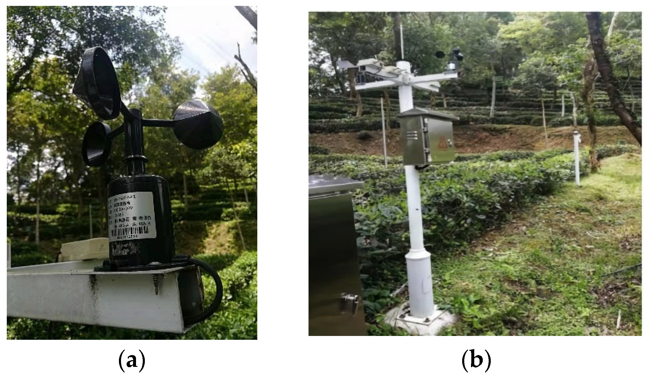
This section details the dataset, CNN-SVM, and LSTM model, including its composition and overall architecture. The application and parameter settings in the experiment are also introduced.

2.1. Dataset

The experimental data were collected in the field with an IoT system at a tea plantation in Huangshan City, Anhui Province. Notably, data were collected for twelve parameters, including time, wind direction, light, air temperature, air humidity, atmospheric pressure, and other environmental information. Additionally, the soil temperature and soil water content at 20 cm, 40 cm, and 60 cm below the surface of the test area at different locations were recorded. The soil temperature and moisture content were measured with an integrated sensor, and there were seven sensors in the system. The sensor collects data every 10 min. A total of 50,455 data points were used in the experiment. Seventy percent of the data were used as the training set, and ten percent of this set consisted of randomly added abnormal values. The remaining 30% of the data were used for testing, and ten percent of this set consisted of randomly added abnormal values. Figure 1 shows part of the collection devices for the data collected in this experiment.

2.2. Data Pre-Processing

2.2.1. Standardization

Different evaluation indexes in a multi-index evaluation system generally have different dimensions and orders of magnitude. If indexes are considerably different and an original index value is used directly for analysis, the result will be biased toward indexes with high values over those with low values. Therefore, to ensure the reliability of the results, it is necessary to standardize index data. This approach can improve the model convergence speed and the model and classifier accuracies.
The most common data standardization methods are min-max standardization and Z-score standardization. This article uses the Z-score standardization method, also known as standard deviation standardization. This method normalizes the data set to the mean and standard deviation of the original data. The standardized data conform to the standard normal distribution; the mean is 0, and the standard deviation is 1. The corresponding conversion function is:
x = x μ / σ
where μ is the mean of all sample data, and σ is the standard deviation. x is the original data, and x is the preprocessed data.

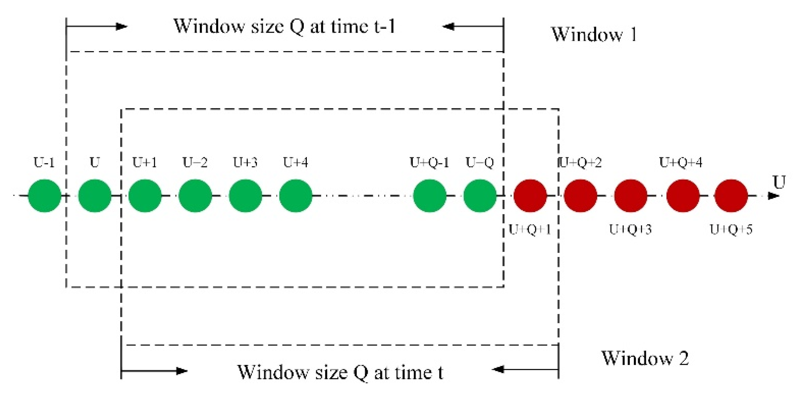
2.2.2. Sliding Window

Time series data processing models usually include landmark, snapshot, and sliding window models. The sliding window model keeps the most recent data in the window, and this approach is more applicable for sensor data than other data stream processing models. Therefore, this paper uses the sliding window model to process IoT time series of data from a tea plantation. The distribution of the collected data may vary over time. Therefore, the sliding window model is used to place newly collected data and the data collected at the previous time step in the same window for the CNN-SVM model to perform anomaly detection. Notably, data detection can be performed online in real-time by moving the window, and the temporal correlation of the data can be used to improve the accuracy of anomaly detection.
The sliding window model is shown in Figure 2. For the convenience of description, it is assumed that the current moment is U, the size of the sliding window is Q, the data set in sliding window 1 is Du = {xU…,xU+Q}, and the data set in window 2 is Du+1 = {xU+1…,xU+1+Q} [32]. In Figure 1, the green dots represent the detected data, and the red dots represent the data to be detected. When new data are collected at the next time step, the window slides to the right; some circles are slid into the window, and some circles are shifted outside the window.
The data in the new window are input into the CNN-SVM model to determine whether they are abnormal data. After many tests (as shown in Table 1), a sliding window size of Q = 7 was established.

2.3. Abnormal Data Detection Model

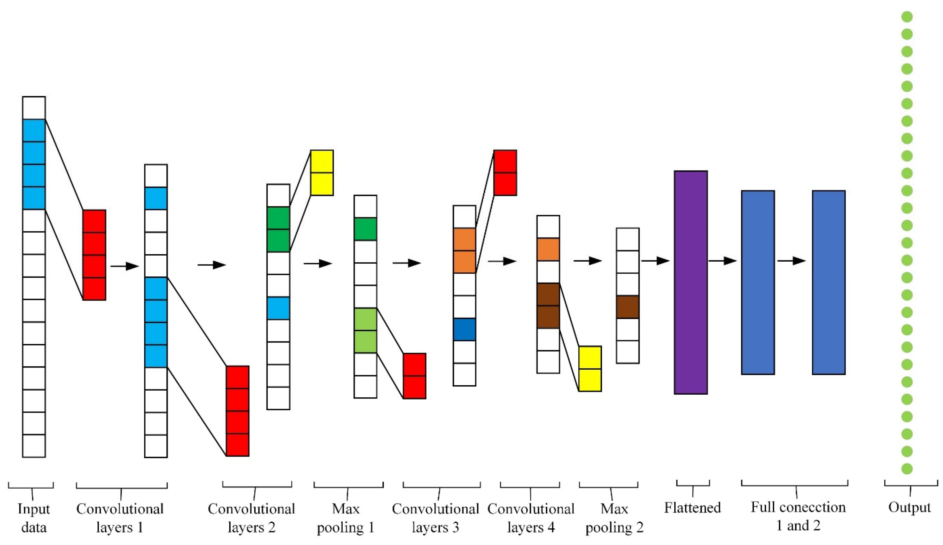
2.3.1. Convolution and Pooling Layer

The convolution kernel of this layer is used to slide the window in the previous level of the input layer, add the offset value, obtain each feature extraction layer through the activation function, and produce the corresponding feature mapping layer [17]. A convolution kernel of a certain size in the convolution layer traverses the input feature map to extract features and performs convolution operations within local areas of the feature map.
The pooling layer, also known as the downsampling layer, uses downsampling to compress dimensions and reduce parameters without affecting the characteristics of the data set [33]. The most common pooling methods are average pooling (average pooling) and maximum pooling (max pooling); this article focuses on max pooling.

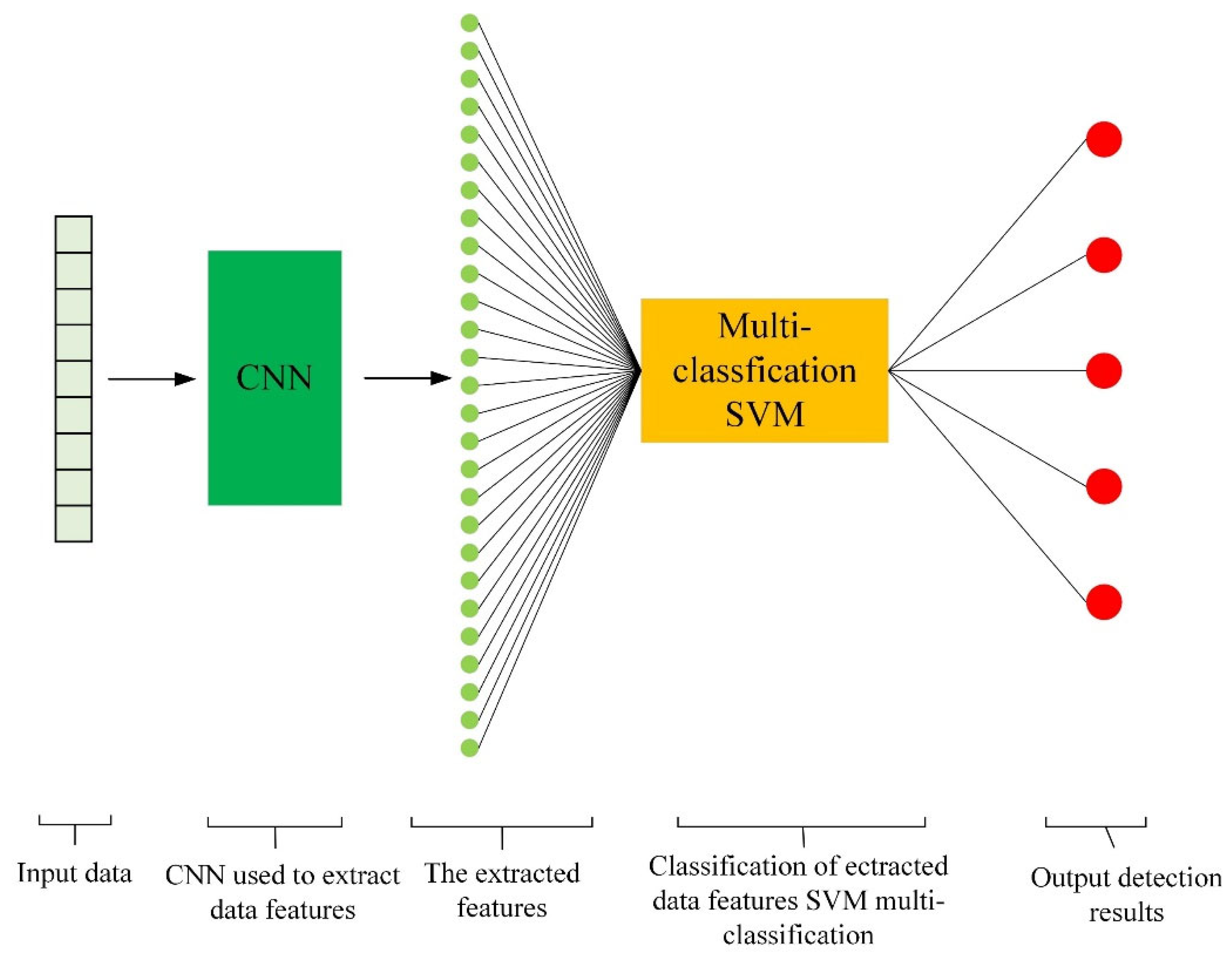
2.3.2. Fully Connected Layer and Support Vector Machine

The fully connected layer is connected to the pooling layer, and the pooled feature map is input into the fully connected layer [34]. An SVM is a machine learning algorithm based on statistical theory and the principle of structural risk minimization. By defining an appropriate kernel function, a nonlinear transformation is performed to transform the input space into a linearly separable high-dimensional space. The optimal linear hyperplane in the high-dimensional space is identified.
A traditional SVM usually solves a two-class classification problem or multiclass classification problem in data anomaly detection, and ‘one-to-one’, ‘one-to-many’, and ‘directed acyclic graph’ methods can be used. This paper adopts the one-to-one method, and a total of N(N-1)/2 subclassifies are constructed for N types of samples. When predicting the category to which a new sample belongs, each subclassifier assesses the sample and casts a vote for the corresponding category. In the final decision stage, the category with the most votes is set as the category of the identified sample [35].

2.3.3. Construction of Exception Data Detection Model

To improve the correlation classification problem involving abnormal data from a tea plantation, a one-dimensional convolutional neural network was selected, and the CNN-SVM model consisting of 8 convolutional, pooling, and fully connected layers was proposed. The model includes three main parts: the input layer, output layer, and hidden layer, as depicted in Figure 3.
First, the time series data are reprocessed, and the processed data are input into the model through the input layer [36]. To classify abnormal data, the activation function of the convolution layer uses the ReLU function, and the scaled exponential linear unit (SeLU) function with normalization is used in the fully connected layer. This is since SeLU can solve the problems of gradient disappearance and explosion very well.
Additionally, the alpha dropout algorithm is selected to accelerate the convergence speed of the model and improve the generalization ability. Alpha dropout is a type of dropout that keeps the input means and variance unchanged. The role of this layer is to maintain the self-standardization of data during dropout through scaling and translation. Additionally, alpha dropout works well with the SeLU activation function. The main parameter settings in the hidden layer are shown in Table 2.
In Table 2, Filter 1 is the number of convolution kernels in convolution layer 1, Filter 2 is the number of convolution kernels in convolution layer 2, and Kernel_size is the length of the convolution window in the convolution layer. Pool_size is the maximum number of windows merged in the largest pooling layer, α is the drop rate in the alpha dropout layer, and Units is the dimension of the output of the fully connected layer.
The data extracted by the dense layer are input into the SVM, and the kernel function of the SVM is the Gaussian radial basis function (RBF). After verification by the K-fold cross-validation algorithm, the penalty factor C = 5.32 , the kernel parameter γ = 2.15 , the OVO classification method, and g a m m a = 0.1 are selected [37]. The smaller the gamma value is, the more continuous the classification interface. The larger the gamma value is, the more scattered the classification interface and the better the classification effect; however, overfitting may occur in this case. ‘OVO’ is a one-to-one classification problem involving division between two categories, and two classification methods are used to simulate the results of multiple classification steps. An objective function (loss function) is introduced to assess the degree of difference between the predicted and actual values. This paper selects the square folded leaf loss function, and regularized penalty terms are added to suppress numerical weights and improve the model generalization ability. The SVM multiclass objective function is given as follows:
L o s s = 1 N i j y i [ m a x ( 0 , f x i ; W j f x i ; W y i + ) ] 2 + λ k l W k , l
where x i is the i t h sample, which is correctly classified as y i ; f x i ; W y i is calculated by the scoring function f for the j t h classification; is the boundary value; the weight is W ; N is the total number of samples, and λ is the penalty factor. The specific flow chart of the CNN-SVM abnormal data detection algorithm is shown in Figure 4.

2.4. Tea Plantation Data Prediction Model
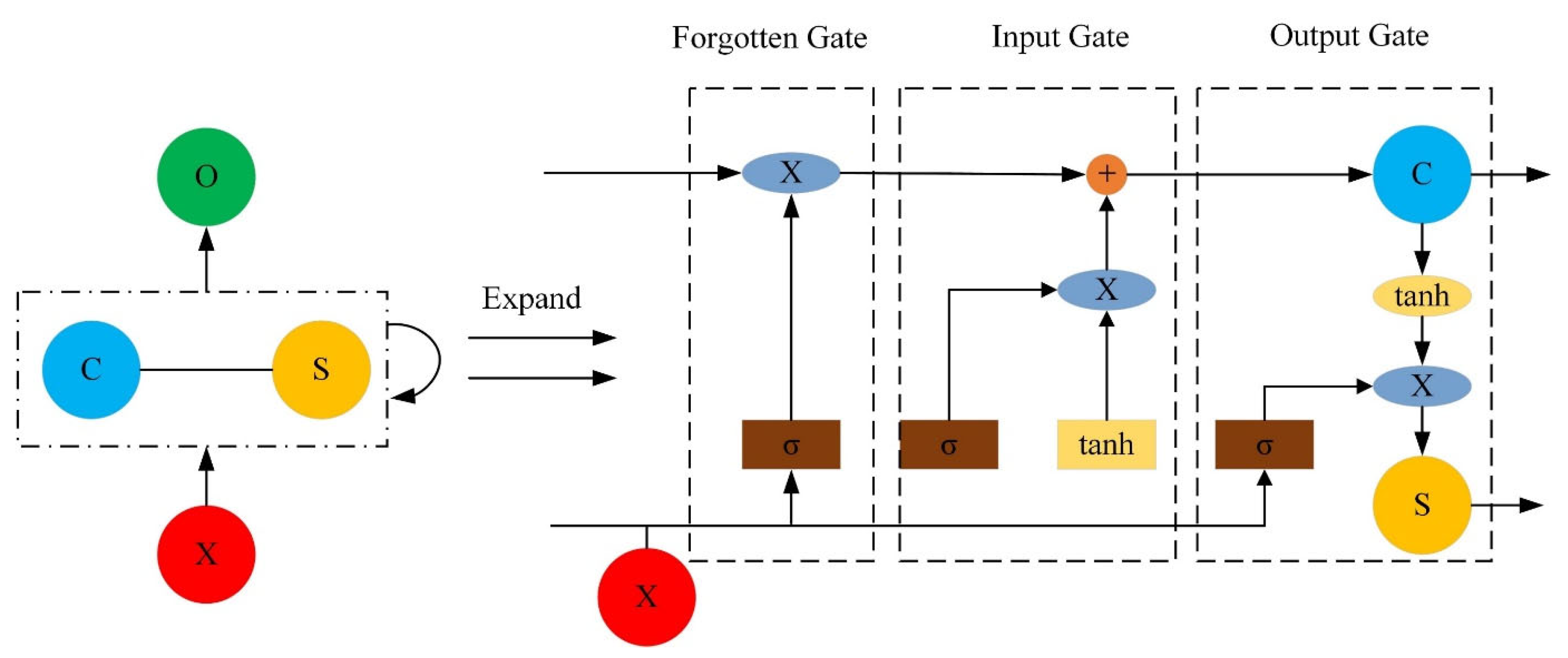
2.4.1. LSTM

To compensate for the shortcoming that ordinary RNNs cannot learn long-distance information, an LSTM model is proposed to predict tea plantation sensor data. An LSTM network is a variant of a recurrent neural network that avoids long-term dependence problems through targeted design. LSTM information is stored in the control unit outside the normal information flow of an RNN; notably, a new state unit is introduced. As shown in Figure 5. LSTM effectively mines the time series dependence of information by adding forget gates, input gates, and output gates to the hidden layer. The core of LSTM design is the threshold mechanism, which involves the abovementioned gates; the functional design of this mechanism can be described as follows.
The input gate i n controls the input layer information that reaches the hidden layer and determines what new information is stored in the new unit state. The corresponding mathematical model is given as follows:
i n = σ U i x n + W i s n 1 + V i c n 1 C n ˜ = t a n h U c x t + W c s n 1
where i n is the input of the input gate at time n, and the information filtered by the input gate is i n C n ˜ . σ is the sigmoid activation function, tanh is the tangent function, U i , U c , W i , W c , V i are the weight matrix, x n is the current input, s n 1 is the output of the previous storage unit, and c n 1 is the original cell state.
The forget gate f n is used to control the storage of information by the current hidden layer node and determine which information is deleted from the memory unit; the mathematical model is given as follows:
f n = σ U f x n + W f s n 1 + V f c n 1
where f n is the threshold for the forget gate, and the information that passes through the forget gate is f n c n 1 .
The output gate o n determines the final output and saves information. The corresponding mathematical model is given as follows:
c n = i n C n ˜ + f n c n 1 o n = σ U o x n + W o s n 1 + V o c n 1 s n = o n t a n h c n
where c n is state c after the forget and input gates, o n is state O for the output layer at time n , and s n is state s in the hidden layer.

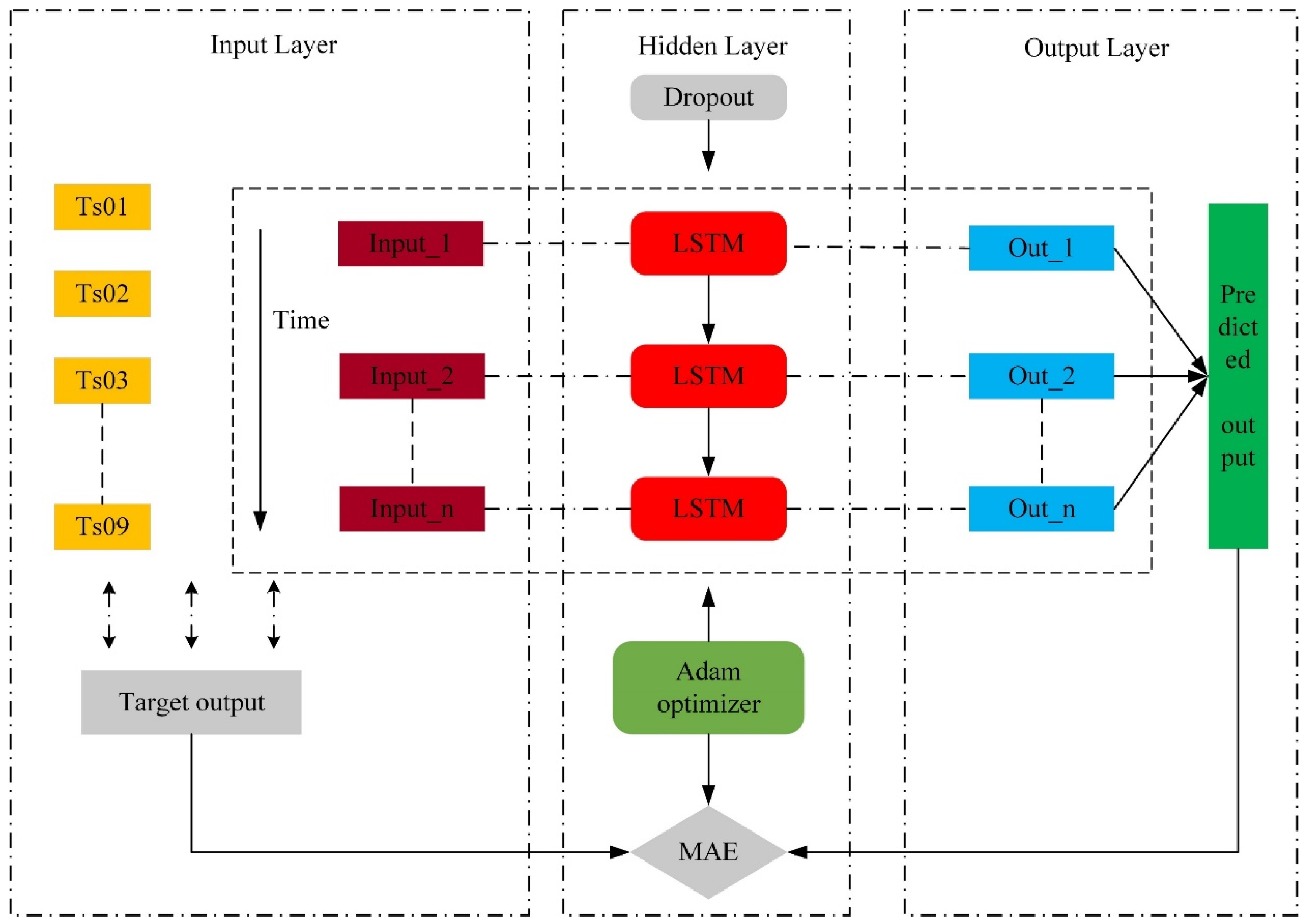
2.4.2. Construction of the Tea Plantation Data Prediction Model

Considering the multivariate correlations among tea plantation data types, an improved multivariate LSTM sensor timing prediction model is proposed. The network structure of this model includes three layers: an input layer, a hidden layer, and an output layer. Among them, the input layer controls the input data format; the hidden layer contains several LSTM units and iteratively adjusts the model weights to reduce the error until convergence is reached, and the output layer restores the format of the result to the original data format. The topological diagram of this model is shown in Figure 6.
Figure 6 shows that the pre-processed sensor data are first converted from the input layer format to data that can be used for supervised learning. Q time points are selected as the interval used in the LSTM model, and the data from T time points are used as the time inputs. The target output is the true value corresponding to an input data time point. Six types of sensors are used to obtain integrated 3D data (time, true value, and features), and time is input as an index in the hidden layer.
The collected tea plantation data sets have strong correlations, so too many hidden layers will lead to overfitting. Therefore, this test uses a double hidden layer structure. Equations (1)–(5) indicate that the choice of the threshold activation function is the key to the success of the experiment because the ReLU function can reduce the problem of gradient dispersion; therefore, the ReLU function is selected as the activation function. To alleviate the impact of overfitting, a dropout algorithm is added to the hidden layer, and the loss function selects the mean absolute error (MAE) function. This function measures the average error margin and is suitable for comparing the average error levels of most models. The optimizer used in the hidden layer is the Adam optimizer, and it optimizes the weights calculated for each loss function until the loss function converges. After model training is completed, the output layer performs denormalization and other processing steps to restore the format of the predicted values to the original data format [38]. The main parameter settings are shown in Table 3.
Among the parameters in Table 3, the number of Units and dropout rate are obtained through grid search, and the search values are 32, 64, 128, 256, and 0.2, 0.3, 0.4, 0.5, 0.6, 0.7, respectively. Use_bias reflects whether the Boolean layer uses the offset vector, and Bias_initializer is the initializer of the offset vector. Unit_forget_bias adds 1 to the bias of the forget gate during initialization. Kernel_initializer is the initializer of the weight matrix and is used for the linear conversion of inputs.

2.5. Evaluation Index of Abnormal Data Detection Algorithm

The traditional indicators of classification algorithm are accuracy, micro-precision, micro-recall, micro-specificity, and the micro-F1 score [39]. The corresponding formulas are shown in Table 4. TP represents a normal value that is correctly predicted; FP represents a normal value that is incorrectly predicted; TN represents an abnormal value that is correctly predicted; FN represents an abnormal value that is incorrectly predicted. TP ¯ ,   FP ¯ ,   TN ¯ ,   and   FN ¯ in Table 4 are the average values of TP, FP, TN, and FN, respectively. Accuracy (ACC) indicates the proportion of all the results of the classification model that are correctly predicted to the total number of observations. Micro-precision (Micro-P) is the proportion of correct normal predictions to the total number of possible normal predictions. Micro-recall represents the proportion of correct normal predictions to the total number of predictions. Micro-specificity refers to the proportion of correct abnormal predictions to the total number of possible abnormal predictions. The micro-F1 score combines the accuracy rate and the output result of micro-recall and reflects the performance of the model. The micro-F1 score ranges from 0 to 1, with 1 representing the best and 0 representing the worst model performance.

2.6. Evaluation Index of Tea Plantation Data Prediction Algorithm

The indicators used to evaluate the prediction performance of the algorithm included the MAE, root mean square error (RMSE), and R squared value (R2) [39]. The formulas for these indexes are shown in Table 5. The MAE is the sum of the absolute values of the deviations of all real values from the corresponding arithmetic averages. MAE can avoid the problem of error cancellation, so it can accurately reflect the actual prediction error. The RMSE represents the degree of dispersion of the predicted values, and the best-fit state is RMSE = 0. R2 reflects the performance of the model, and the value range is [0, 1]. A value of 0 represents the worst model-fitting ability, and 1 represents the best model-fitting ability. In Table 5, Y i is the true value, Y ^ i   is the predicted value, and Y i ¯ is the mean value.

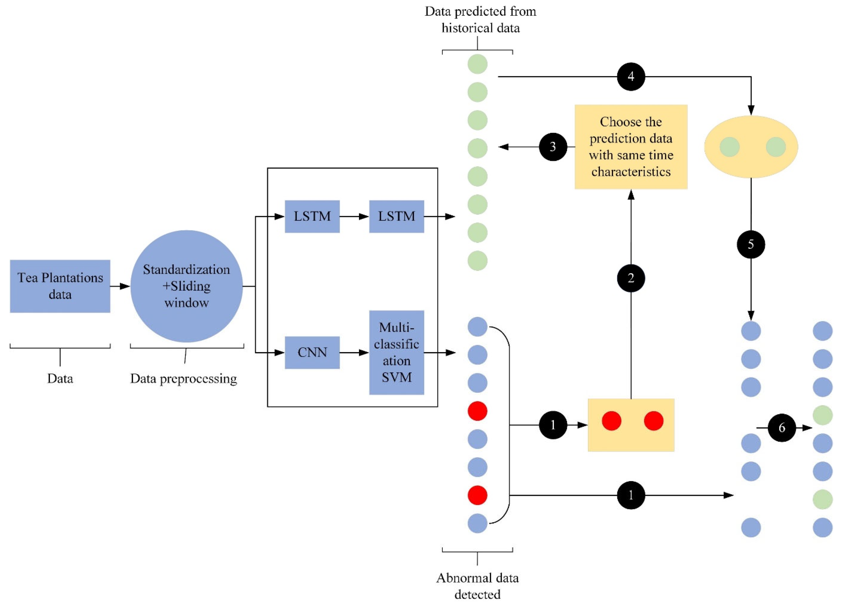
2.7. Correction Model of Abnormal Data in Tea Plantations

Based on the abnormal data detection and prediction methods proposed in Section 2.2 and Section 2.3, a model for correcting abnormal data with predicted values is designed. The model is divided into three parts. The first part is the abnormal data detection stage. The CNN-SVM model is obtained by training the data collected at the tea plantation, which are used to detect abnormal data. The second part is the data prediction stage. It includes model training with historical tea plantation data to obtain an LSTM model that can accurately predict future tea plantation data. The third part is the correction stage. If the CNN-SVM model detects abnormal data, the data predicted by the LSTM model are used to correct the abnormal data. This paper addresses the detection, prediction, and correction of IoT anomalous data in tea plantations, which helps in the intelligent management of tea plantations, scientific irrigation, and other efforts. Thus, only the data accuracy of the IoT system was improved in this research, but the tea yield and other issues are affected indirectly.
Figure 7 shows the overall structure of the abnormal data correction model. The historical tea plantation data are pre-processed by normalization and time slicing into the CNN-SVM model and the LSTM model for data detection and prediction. If the detected data are normal, they are output to the tea plantation data set. If the detected data are abnormal, these data are retained, and the time points T of the abnormal data are extracted. Then, the LSTM model predicts the data at time T and corrects the abnormal data. The result is input into the tea plantation data set.

3. Results and Discussion

This section introduces the anomaly data detection model is compared and analyzed by the CNN-SVM and CNN models. The results of the tea plantation data prediction model and abnormal data model correction are analyzed.

3.1. Results

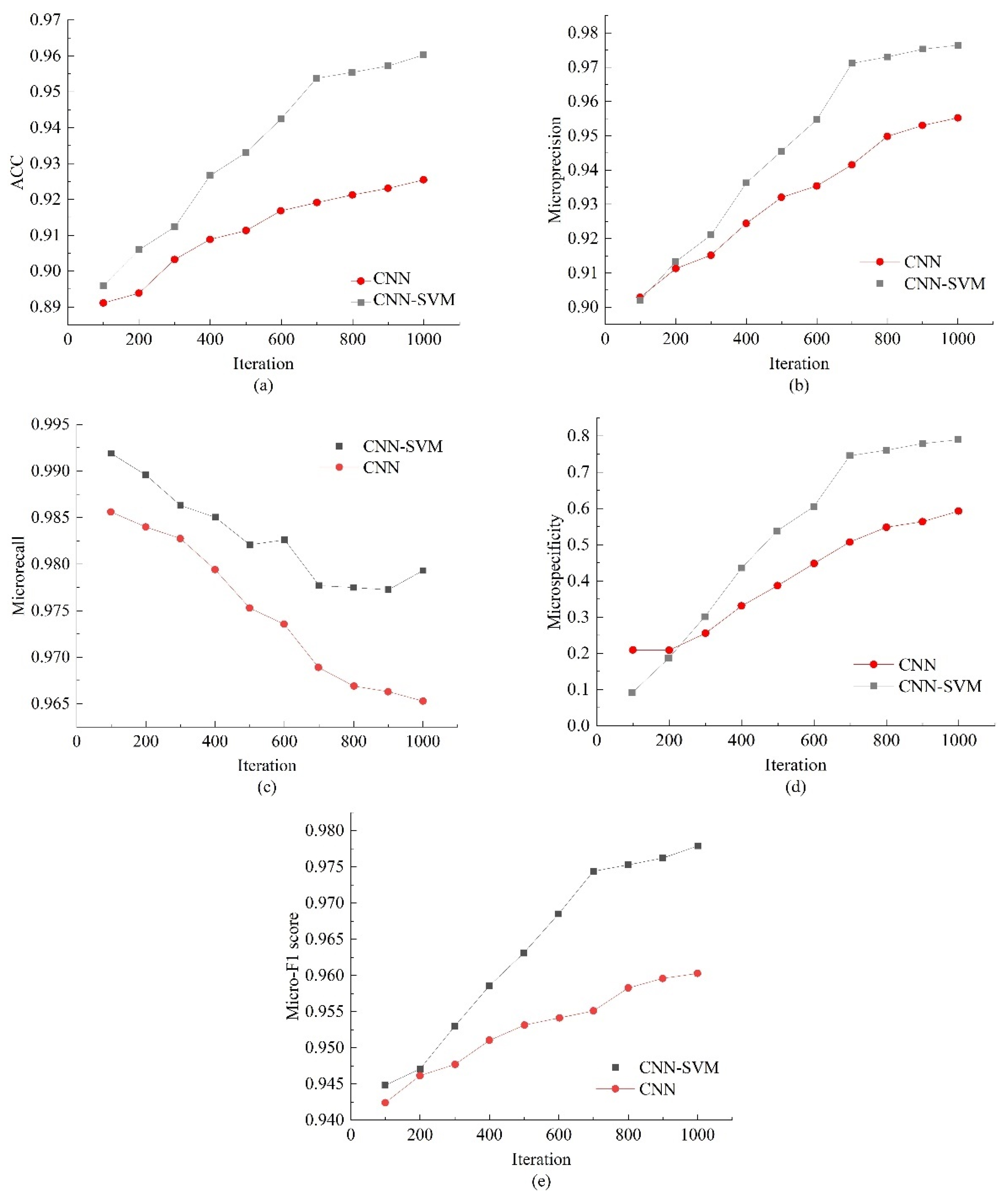
3.1.1. Results of the Abnormal Data Detection Algorithm

The curve in Figure 8 shows the variation in the training data’s loss values and the CNN-SVM model’s testing data. Figure 8 indicates that when the number of iterations reaches 700, the training and testing data loss function values are close to 0.2386. Subsequently, the value of the loss function decreases. When the number of iterations reaches 800, the value of the loss function stabilizes at 0.1987. In the interval of [0, 700] iterations, the value of the loss function also decreases rapidly. The loss value decreases slowly in the interval of (700, 900) iterations. In the interval of (900, 1000) iterations, the loss function fluctuates near approximately 0.188 8 and tends to be stable.
Figure 9 gives a comparison of the performance of the classification results for the CNN and CNN-SVM models for the studied dataset. Figure 9a compares the changes in the accuracy of the two models for the same ratio dimension and the same data set. Notably, as the number of iterations increases, the accuracy of the model improves. In the process, the highest accuracies of the CNN and CNN-SVM models are 92.55% and 96.02%, respectively. Compared with the CNN model, the detection accuracy of the CNN-SVM model is approximately 3.5% higher. Figure 9b shows the Micro-P of the two models at different iteration times. Notably, the Micro-P values of the CNN-SVM model are better than those of the CNN model, and the two result sets are similar only in the interval of [0, 100] iterations. The gap is largest at the 700th iteration and then tends to stabilize.
Figure 9 gives a comparison of the performance of the classification results for the CNN and CNN-SVM models for the studied data set. Figure 9a compares the changes in the accuracy of the two models for the same ratio dimension and data set. Notably, as the number of iterations increases, the accuracy of the model improves. In the process, the highest accuracies of the CNN and CNN-SVM models are 92.55% and 96.02%, respectively. Compared with the CNN model, the detection accuracy of the CNN-SVM model is approximately 3.5% higher. Figure 9b shows the Micro-P of the two models at different iteration times. Notably, the Micro-P values of the CNN-SVM model are better than those of the CNN model, and the two result sets are similar only in the interval of [0, 100] iterations. The gap is largest at the 700th iteration and then tends to stabilize.
Figure 9c,d show the changes in the micro-recall and micro-specificity of the two models, respectively. Specifically, as the number of iterations increases, the micro-recall rate of the CNN model tends to be stable at 96.63%, and that of the CNN-SVM model tends to be stable at 97.72%. The final micro-recall rate of the CNN-SVM model is 97.93%, and the micro-specificity is 78.78%. The final micro-recall rate of the CNN model is 96.63%, and the micro-specificity is 56.71%. Compared with that of the CNN model, the micro-recall rate of the CNN-SVM model is approximately 1.3% higher, and the micro-specificity is approximately 22.2% higher. Figure 9e shows the change in Micro-F1 as the number of iterations increases in the two models. After the 800th iteration, the Micro-F1 results gradually stabilize. The final Micro-F1 value of the CNN-SVM model is 97.79%, and that for the CNN model is 96.03%.
In summary, based on evaluations of ACC, Micro-P, micro-recall, micro-specificity, and the micro-F1 score, the detection results of the CNN-SVM model are significantly better than those of the CNN model.

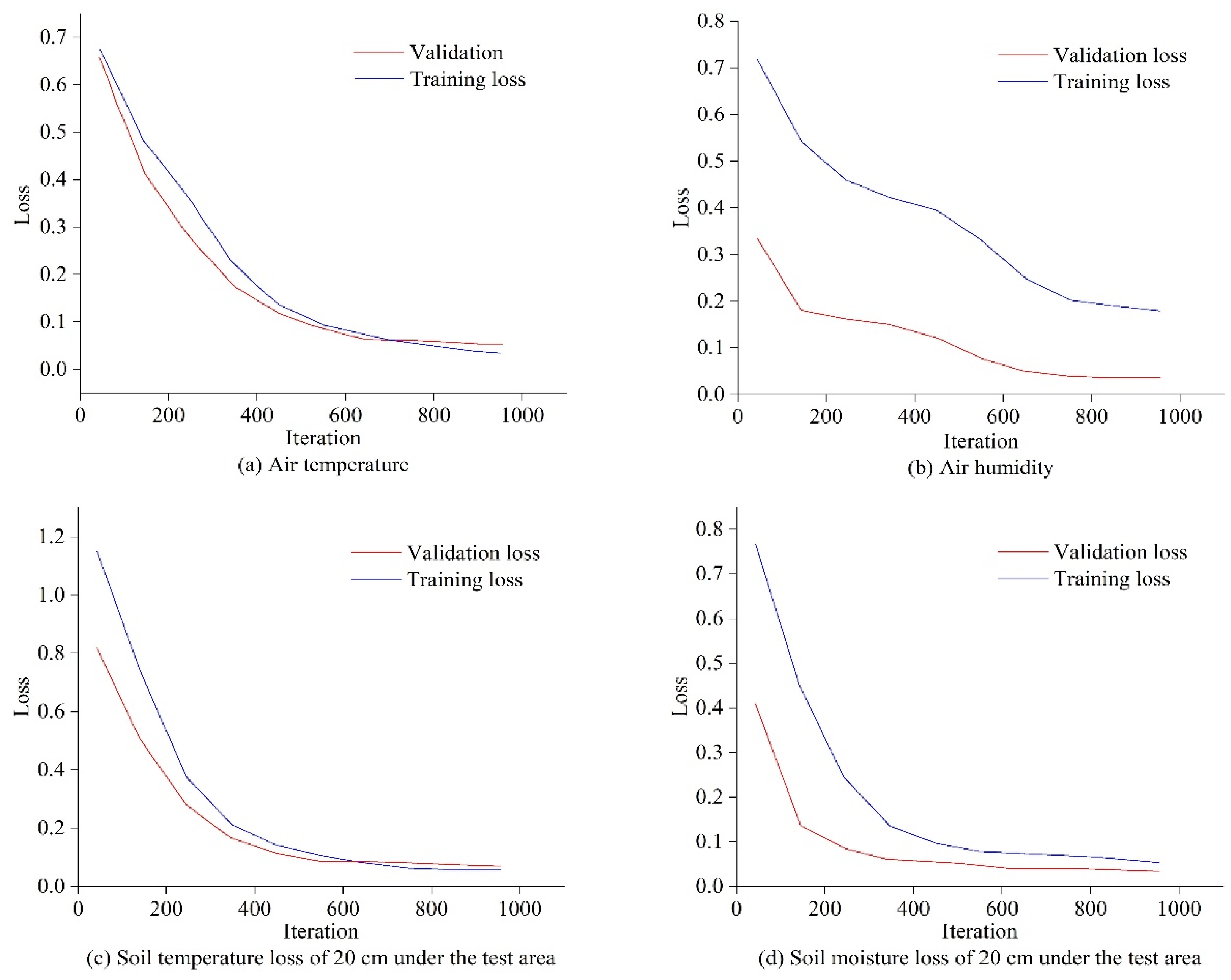
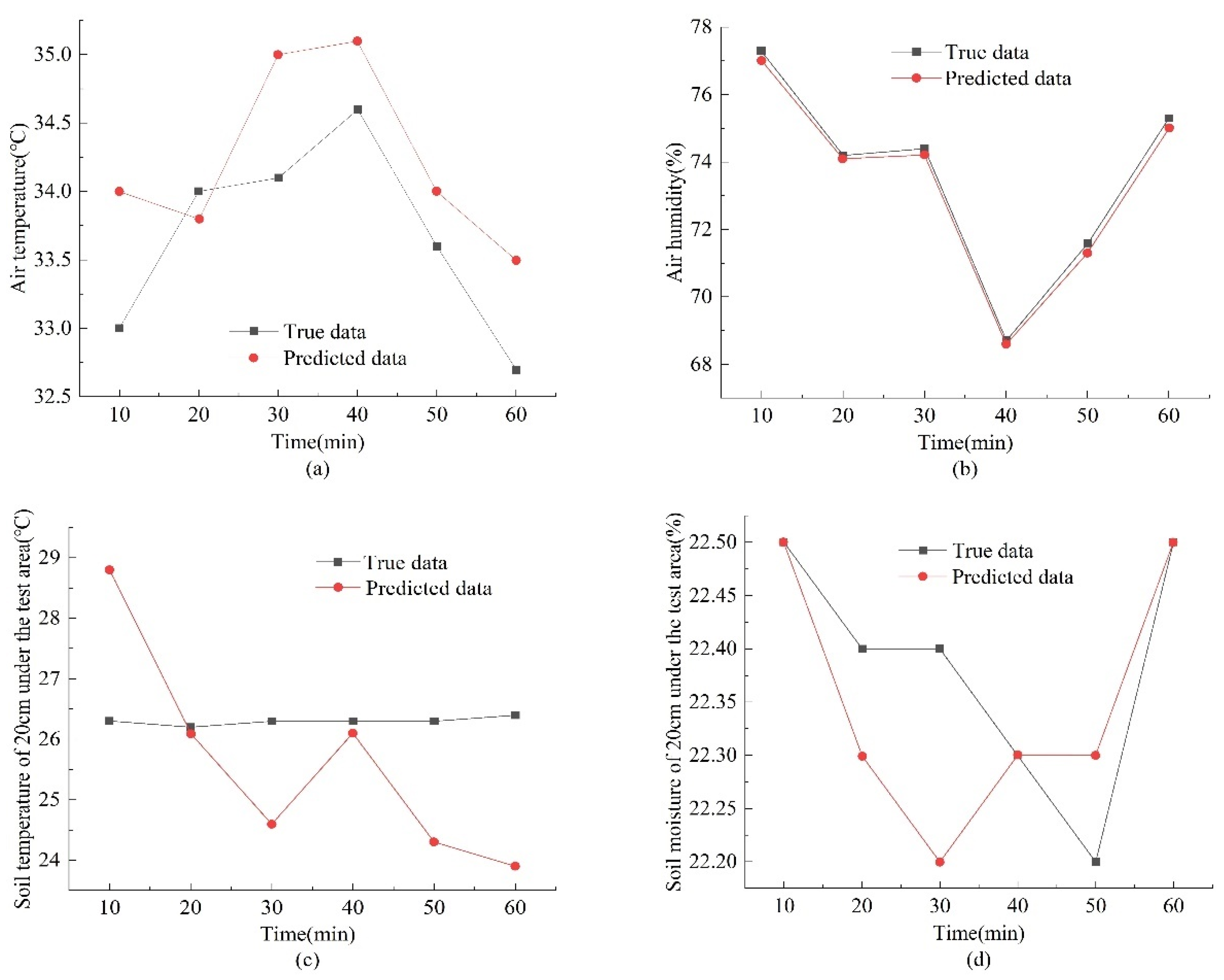
3.1.2. Results of Data Prediction Algorithm of Tea Plantations

The prediction results are shown in Figure 10 and Figure 11. Twelve-hour data are selected as the observation data set, and 1-h data forecasts are produced. Because the data are collected every 10 min, 72 data points are needed as observations, and 6 data points are predicted. Figure 10 shows the change in the obtained loss function value, and Figure 11 shows a comparison between the predicted and real values.
Figure 10 shows that the LSTM model training and prediction results are good. Except for the air humidity loss, which converges at approximately 800 iterations, the remaining three sets of variables all begin to converge around the 400th iteration, and the final loss is in the [0, 0.1] interval. To verify the prediction results, Figure 11 intuitively shows the prediction effect, where the red dots are the true values, the blue dots are the predicted values, and the broken blue line is the observation data. In hour-ahead forecasting, the air humidity and soil moisture 20 cm below the experimental area’s surface best fit the actual data. Additionally, the soil temperature 20 cm below the experimental area’s surface needs to be a better fit for the actual data, and the air temperature prediction performance could be better.
Table 6 shows the changes in MAE, RMSE, and R2 of the LSTM model as the number of iterations increases. As can be seen from the table, when iterating 1000 times, MAE, RMSE, and R2 perform best at 0.0022, 0.0148 and 0.9669, respectively. Additionally, the correction results are shown in Figure 12.

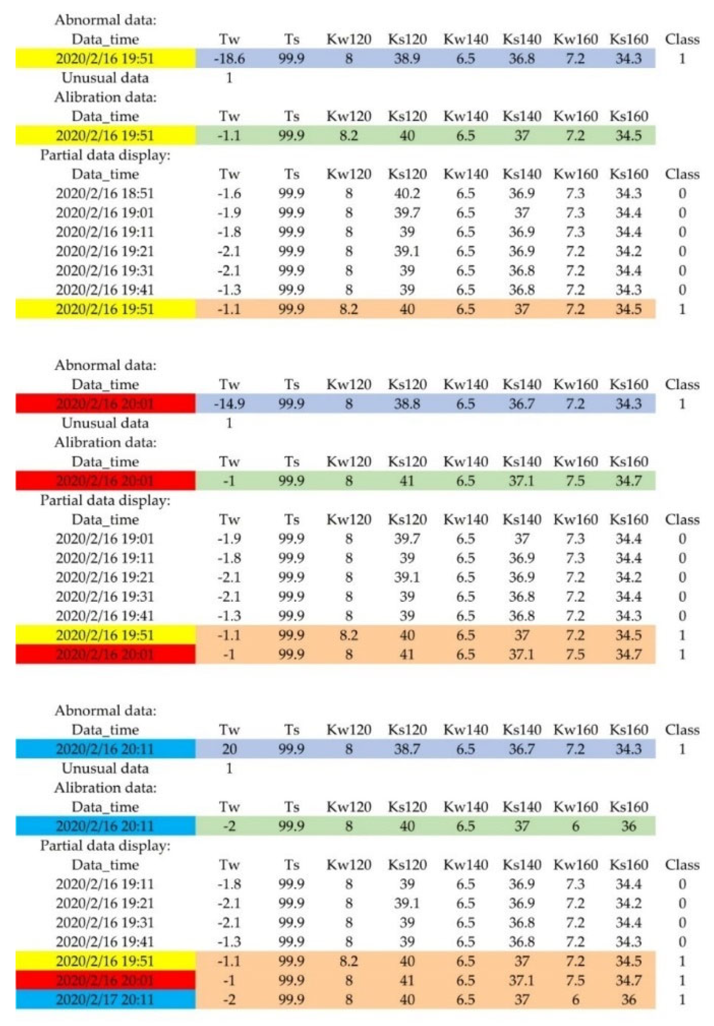
3.1.3. Results of Abnormal Data Correction

As shown in Figure 12, Data_time is the data collection time, and Tw and Ts represent the air temperature and air humidity, respectively. Kw120, Kw140, and Kw160 are the soil temperatures 20 cm, 40 cm, and 60 cm below the experimental area, respectively, and Ks120, Ks140, and Ks160 are the soil moisture contents 20 cm, 40 cm, and 60 cm below the experimental area, respectively. In Figure 12, the light blue box represents the abnormal data detected by the CNN-SVM model, the green box represents the predicted data of the LSTM network, and the orange box is the corrected dataset. Red, yellow and blue boxes are abnormal data time points. Figure 12 indicates that when abnormal data are detected, the system extracts the time points of the abnormal data and simultaneously extracts the corresponding predicted data according to these time points for correction. The system will automatically store abnormal data.

3.2. Discussion

In this subsection, the method proposed in this study is compared with other methods for anomalous data detection, such as support vector machine (SVM) [40], local anomaly factor (LOF) [41], and isolated forest (IForest) [42]. As observed in Table 7, the CNN-SVM model proposed in this research can be optimal in most categories of data detection but only in some categories of anomalous data detection in IoT of tea plantations. This may be due to the fact that CNN-SVM extracts features from the data better than traditional machine algorithms and performs well with multi-dimensional data. Although SVM and Iforest achieve optimal results under a certain measure, our proposed method is more widely applicable. Therefore, in future work, this study can go more deeply into the model research for a certain class of anomalous data detection, and combine CNN with more machine algorithms to obtain further results. Table 8 shows the comparison of the prediction performance of LSTM and RNN [26]. It can be seen that LSTM has a higher performance. Since LSTM can better handle long-term information and avoid the gradient disappearance that often occurs in RNNs, LSTM achieves optimality in every measure.
In the actual conditions, the real data obtained will be interfered with by kinds of conditions (such as wind speed, wind direction, sudden changes, etc.) then our predicted values will be biased. However, replacing the anomalous values with our predicted values is more scientific and effective than removing them directly. The model proposed in this study performs detection and prediction once every 60 min, as a shorter detection period is better for the timely detection of anomalous data. In our future work, we will select appropriate time intervals for detection and prediction and further consider potential factors such as prediction accuracy and robustness.

4. Conclusions and Future Work

To address issues associated with abnormal data collected by tea plantation sensors, this paper proposes a high-dimensional time series correction algorithm for abnormal data based on deep learning. This approach has the following advantages:
  • Based on standardized data processing, the algorithm uses a CNN-SVM model with a sliding window to monitor the processed data online. The results show that compared with the traditional CNN model for anomaly detection algorithm, the proposed algorithm can obtain better detection results, with accuracy and micro-specificity improvements of 3–4% and 20–30%, respectively.
  • An abnormal data correction method based on an LSTM model is proposed. This algorithm predicts the trends in abnormal data based on multifactor historical data, which effectively improves the detection accuracy of the model for time series of data. When the anomaly detection algorithm detects abnormal data, the time points of the anomalous data are extracted, normal data are predicted with the LSTM model, and the abnormal data are corrected and added to the tea plantation data set.
  • This paper’s CNN-SVM model and LSTM model are versatile and easy to combine with other algorithms. Although this research focuses on a tea plantation, the proposed method provides an important reference for detecting and processing sensor data.
In future research, the simultaneous failure of multiple sensors will be considered to improve the versatility of the model. Additionally, the improved LSTM model or other machine learning algorithms will be used to correct abnormal data to improve the accuracy of data correction.

Author Contributions

Methodology, J.F. and G.Z.; investigation, B.L., S.X. and Y.H.; resources, L.Z.; data curation, Y.L., Z.Z. and X.W.; writing—original draft preparation, R.W. and T.W.; writing—review and editing, W.Z.; visualization, C.Z. All authors have read and agreed to the published version of the manuscript.

Funding

This research received no external funding.

Acknowledgments

This work was supported by the Independent Project of Anhui Key Laboratory of Smart Agricultural Technology and Equipment (grant no. APKLSATE2019X001), and the Key Research and Development Projects of Anhui Province (grant no. 201904a06020056, 202104a06020012, 202204c06020022). Special thanks to Feng J for his contribution to this paper.

Conflicts of Interest

The authors declare no conflict of interest.

References

  1. Ma, J.; Sun, L.; Wang, H.; Zhang, Y.; Aickelin, U. Supervised anomaly detection in uncertain pseudoperiodic data streams. ACM Trans. Internet Technol. 2016, 16, 1–20. [Google Scholar] [CrossRef] [Green Version]
  2. Kim, M.; Ou, E.; Loh, P.L.; Allen, T.; Agasie, R.; Liu, K. RNN-Based online anomaly detection in nuclear reactors for highly imbalanced datasets with uncertainty. Nucl. Eng. Des. 2020, 364, 110699. [Google Scholar] [CrossRef]
  3. Ahmed, M.; Mahmood, A.N.; Islam, M.R. A survey of anomaly detection techniques in financial domain. Futur. Gener. Comput. Syst. 2016, 55, 278–288. [Google Scholar] [CrossRef]
  4. Chen, Q.; Lam, K.Y.; Fan, P. Comments on “Distributed Bayesian algorithms for fault-tolerant event region detection in wireless sensor networks”. IEEE Trans. Comput. 2005, 54, 1182–1183. [Google Scholar] [CrossRef]
  5. Limthong, K.; Fukuda, K.; Ji, Y.; Yamada, S. Unsupervised learning model for real-time anomaly detection in computer networks. IEICE Trans. Inf. Syst. 2014, E97-D, 2084–2094. [Google Scholar] [CrossRef] [Green Version]
  6. Liu, C.; Gryllias, K. A semi-supervised Support Vector Data Description-based fault detection method for rolling element bearings based on cyclic spectral analysis. Mech. Syst. Signal Process. 2020, 140, 106682. [Google Scholar] [CrossRef]
  7. Ghorbel, O.; Ayedi, W.; Snoussi, H.; Abid, M. Fast and efficient outlier detection method in wireless sensor networks. IEEE. Sens. J. 2015, 15, 3403–3411. [Google Scholar] [CrossRef]
  8. Samparthi VS, K.; Verma, H.K. Outlier detection of data in wireless sensor networks using kernel density estimation. Int. J. Comput. Appl. 2010, 5, 28–32. [Google Scholar] [CrossRef]
  9. Passalis, N.; Tsantekidis, A.; Tefas, A.; Kanniainen, J.; Gabbouj, M.; Iosifidis, A. Time-series classification using neural bag-of-features. In Proceedings of the 2017 25th European Signal Processing Conference (EUSIPCO), Kos, Greece, 28 August–2 September 2017; pp. 301–305. [Google Scholar]
  10. Jin, C.-B.; Li, S.; Do, T.D.; Kim, H. Real-time human action recognition using CNN over temporal images for static video surveillance cameras. In Pacific Rim Conference on Multimedia; Springer: Cham, Switzerland, 2015; pp. 330–339. [Google Scholar]
  11. Jiang, Z.; Li, T.; Min, W.; Qi, Z.; Rao, Y. Fuzzy c-means clustering based on weights and gene expression programming. Pattern Recognit. Lett. 2017, 90, 1–7. [Google Scholar] [CrossRef]
  12. Xu, R.; Cheng, Y.; Liu, Z.; Xie, Y.; Yang, Y. Improved Long Short-Term Memory based anomaly detection with concept drift adaptive method for supporting IoT services. Futur. Gener. Comput. Syst. 2020, 112, 228–242. [Google Scholar] [CrossRef]
  13. Xu, C.; Chen, H. A hybrid data mining approach for anomaly detection and evaluation in residential buildings energy data. Energy Build. 2020, 215, 109864. [Google Scholar] [CrossRef]
  14. Androulidakis, G.; Chatzigiannakis, V.; Papavassiliou, S. Network anomaly detection and classification via opportunistic sampling. IEEE Netw. 2009, 23, 6–12. [Google Scholar] [CrossRef]
  15. Xu, X. Sequential anomaly detection based on temporal-difference learning: Principles, models and case studies. Appl. Soft Comput. J. 2010, 10, 859–867. [Google Scholar] [CrossRef]
  16. Janke, J.; Castelli, M.; Popovič, A. Analysis of the proficiency of fully connected neural networks in the process of classifying digital images: Benchmark of different classification algorithms on high-level image features from convolutional layers. Expert Syst. Appl. 2019, 135, 12–38. [Google Scholar] [CrossRef] [Green Version]
  17. Kumar, A.; Gandhi, C.P.; Zhou, Y.; Kumar, R.; Xiang, J. Improved deep convolution neural network (CNN) for the identification of defects in the centrifugal pump using acoustic images. Appl. Acoust. 2020, 167, 107399. [Google Scholar] [CrossRef]
  18. Eapen, J.; Bein, D.; Verma, A. Novel deep learning model with CNN and bi-directional LSTM for improved stock market index prediction. In Proceedings of the 2019 IEEE 9th Annual Computing and Communication Workshop and Conference (CCWC), Las Vegas, NV, USA, 7–9 January 2019; pp. 264–270. [Google Scholar] [CrossRef]
  19. Krizhevsky, A.; Sutskever, I.; Hinton, G.E. Imagenet classification with deep convolutional neural networks. Adv. Neural Inf. Process. Syst. 2012, 25, 1097–1105. [Google Scholar] [CrossRef] [Green Version]
  20. He, K.; Zhang, X.; Ren, S.; Sun, J. Deep residual learning for image recognition. In Proceedings of the IEEE Conference on Computer Vision and Pattern Recognition, Las Vegas, NV, USA, 27–30 June 2016; pp. 770–778. [Google Scholar]
  21. Rehman, A.; Saba, T.; Kashif, M.; Fati, S.M.; Bahaj, S.A.; Chaudhry, H. A revisit of internet of things technologies for monitoring and control strategies in smart agriculture. Agronomy 2022, 12, 127. [Google Scholar] [CrossRef]
  22. Khan, M.A.; Akram, T.; Sharif, M.; Awais, M.; Javed, K.; Ali, H.; Saba, T. CCDF: Automatic system for segmentation and recognition of fruit crops diseases based on correlation coefficient and deep CNN features. Comput. Electron. Agric. 2018, 155, 220–236. [Google Scholar] [CrossRef]
  23. Wang, R.; Zhang, W.; Ding, J.; Xia, M.; Wang, M.; Rao, Y.; Jiang, Z. Deep Neural Network Compression for Plant Disease Recognition. Symmetry 2021, 13, 1769. [Google Scholar] [CrossRef]
  24. Hinton, G.; Deng, L.; Yu, D.; Dahl, G.E.; Mohamed, A.-R.; Jaitly, N.; Senior, A.; Vanhoucke, V.; Nguyen, P.; Sainath, T.N.; et al. Deep neural networks for acoustic modeling in speech recognition: The shared views of four research groups. IEEE Signal Process. Mag. 2012, 29, 82–97. [Google Scholar] [CrossRef]
  25. Young, T.; Hazarika, D.; Poria, S.; Cambria, E. Recent trends in deep learning based natural language processing. IEEE Comput. Intell. Mag. 2018, 13, 55–75. [Google Scholar] [CrossRef]
  26. Ma, W. Analysis of anomaly detection method for Internet of things based on deep learning. Trans. Emerg. Telecommun. Technol. 2020, 31, e3893. [Google Scholar] [CrossRef]
  27. Ji, C.; Lu, S. Exploration of marine ship anomaly real-time monitoring system based on deep learning. J. Intell. Fuzzy Syst. 2020, 38, 1235–1240. [Google Scholar] [CrossRef]
  28. Zhang, Y.; Chen, X.; Jin, L.; Wang, X.; Guo, D. Network intrusion detection: Based on deep hierarchical network and original flow data. IEEE Access 2019, 7, 37004–37016. [Google Scholar] [CrossRef]
  29. Liu, Q.; Wu, Y.; Jun, Z.; Li, X. Deep learning in the information service system of agricultural Internet of Things for innovation enterprise. J. Supercomput. 2022, 78, 5010–5028. [Google Scholar] [CrossRef]
  30. Jin, X.B.; Yu, X.H.; Wang, X.Y.; Bai, Y.T.; Su, T.L.; Kong, J.L. Deep learning predictor for sustainable precision agriculture based on internet of things system. Sustainability 2020, 12, 1433. [Google Scholar] [CrossRef] [Green Version]
  31. Jin, X.B.; Yang, N.X.; Wang, X.Y.; Bai, Y.T.; Su, T.L.; Kong, J.L. Hybrid deep learning predictor for smart agriculture sensing based on empirical mode decomposition and gated recurrent unit group model. Sensors 2020, 20, 1334. [Google Scholar] [CrossRef] [PubMed] [Green Version]
  32. Jin, P.; Xia, X.; Qiao, Y.; Cui, X. High-dimensional data anomaly detection for wsns based on deep belief network. Chin. J Sens. Actuators 2019, 32, 892–901. [Google Scholar] [CrossRef]
  33. Wang, X.F.; Sun, X.M.; Fang, Y. Genetic algorithm solution for multi-period two-echelon integrated competitive/uncompetitive facility location problem. Asia-Pac. J. Oper. Res. 2008, 25, 33–56. [Google Scholar] [CrossRef]
  34. Pittino, F.; Puggl, M.; Moldaschl, T.; Hirschl, C. Automatic anomaly detection on in-production manufacturing machines using statistical learning methods. Sensors 2020, 20, 2344. [Google Scholar] [CrossRef] [Green Version]
  35. Munir, M.; Siddiqui, S.A.; Dengel, A.; Ahmed, S. DeepAnT: A Deep Learning Approach for Unsupervised Anomaly Detection in Time Series. IEEE Access 2019, 7, 1991–2005. [Google Scholar] [CrossRef]
  36. Canizo, M.; Triguero, I.; Conde, A.; Onieva, E. Multi-head CNN–RNN for multi-time series anomaly detection: An industrial case study. Neurocomputing 2019, 363, 246–260. [Google Scholar] [CrossRef]
  37. Hsu, C.W.; Chang, C.C.; Lin, C.J. A practical guide to support vector classification. 2003. [Google Scholar]
  38. Ravanbakhsh, M.; Nabi, M.; Mousavi, H.; Sangineto, E.; Sebe, N. Plug-and-play cnn for crowd motion analysis: An application in abnormal event detection. In Proceedings of the 2018 IEEE Winter Conference on Applications of Computer Vision (WACV), Lake Tahoe, NV, USA, 12–15 March 2018; pp. 1689–1698. [Google Scholar]
  39. Zheng, Q.; Tasian, G.; Fan, Y. Transfer learning for diagnosis of congenital abnormalities of the kidney and urinary tract in children based on ultrasound imaging data. In Proceedings of the 2018 IEEE 15th International Symposium on Biomedical Imaging (ISBI 2018), Washington, DC, USA, 4–7 April 2018. [Google Scholar]
  40. Fang, W.; Tan, X.; Wilbur, D. Application of intrusion detection technology in network safety based on machine learning. Saf. Sci. 2020, 124, 104604. [Google Scholar] [CrossRef]
  41. Sun, S.; Li, G.; Chen, H.; Guo, Y.; Wang, J.; Huang, Q.; Hu, W. Optimization of support vector regression model based on outlier detection methods for predicting electricity consumption of a public building WSHP system. Energy Build. 2017, 151, 35–44. [Google Scholar] [CrossRef]
  42. Xing, G.; Chen, J.; Hou, R.; Zhou, L.; Dong, M.; Zeng, D.; Luo, J.; Ma, M. Isolation Forest-Based Mechanism to Defend against Interest Flooding Attacks in Named Data Networking. IEEE Commun. Mag. 2021, 59, 98–103. [Google Scholar] [CrossRef]
Figure 1. Environment and equipment of tea plantation. (a) a wind speed monitor; (b) a small agricultural weather station.
Agriculture 13 00480 g001
Figure 2. Sliding window model.
Agriculture 13 00480 g002
Figure 3. CNN extracted data feature structure map from the CNN-SVM model. The number of filters in the first two layers is 64, and in the latter two layers is 32. The first two filters have size 4; the last two have size 2. The window size of the maximum pool layer is 2. The activation function of the fully connected layer adopts the SeLU function.
Agriculture 13 00480 g003
Figure 4. CNN-SVM Model for Detection of Abnormal Data in IoT in Tea Plantations.
Agriculture 13 00480 g004
Figure 5. LSTM network design structure. It introduces the cell state C to store the long-term information of the sequence, and S is the output of the current storage cell. σ represents the sigmoid activation function, while × and + represent the matrix multiplication and addition, respectively.
Agriculture 13 00480 g005
Figure 6. LSTM topological structure diagram.
Agriculture 13 00480 g006
Figure 7. Abnormal Data Detection and Correction Model Structure Chart.
Agriculture 13 00480 g007
Figure 8. The change in values in the CNN-SVM model loss training and testing set.
Agriculture 13 00480 g008
Figure 9. CNN-SVM and CNN performance comparison plots. (a) CNN and CNN-SVM accuracy comparison. (b) CNN and CNN-SVM micro-precision comparison. (c) CNN and CNN-SVM micro-recall comparison. (d) CNN and CNN-SVM micro-specificity comparison. (e) CNN and CNN-SVM micro-F1 scores comparison.
Agriculture 13 00480 g009
Figure 10. Variations in the loss function results for various sensors.
Agriculture 13 00480 g010
Figure 11. Comparison of LSTM Model Forecast and Real Value. (a) Comparison of predicted and real air temperatures over the next hour. (b) Comparison of predicted and true air humidity values over the next hour. (c) Comparison of predicted and true soil temperatures of 20 cm in the experimental area over the next hour. (d) Comparison of predicted and true soil moisture values for 20 cm in the experimental area over the next hour.
Agriculture 13 00480 g011
Figure 12. Results of abnormal data correction.
Agriculture 13 00480 g012
Table 1. Determine the sliding window size.
Sliding Window SizeCorrect Rate for 100 Rounds of Training (Accuracy)Correct Rate for 500 Rounds of Training (Accuracy)
Q = 7 89.350%96.002%
Q = 8 89.450%95.996%
Q = 9 89.470%96.101%
Q = 10 89.330%95.990%
Q = 11 89.310%95.938%
Table 2. Partial parameter setting for the abnormal data detection model.
Title 1Title 2
Filter64
Kernel_size 14
α 0.6
Filter 264
Pool_size2
Units128
Learning rate0.001
Filter 332
Filter 432
Kernel_size 22
Table 3. Partial parameter settings for the Tea Plantation Data Prediction Model.
Parameter NameValue
Unit 1128
Unit 264
Unit 38
Bias_initializerzeros
Dropout0.5
Use_biasTrue
Unit_forget_biasTure
Kernel_initializerglorot_unfiprm
Learning rate0.001
Table 4. Classification algorithm performance indicators.
Formula
Accuracy A c c u r a c y = T P + T N T P + T N + F P + F N × 100 %
Micro-precision M i c r o P = T P ¯ T P ¯ + F P ¯ × 100 %
Micro-recall M i c r o R =   T P ¯ T P ¯ + F N ¯ × 100 %
Micro-specificity M i c r o S = T N ¯ T N ¯ + F P ¯ × 100 %
Micro-F1 score F 1   S c o r e = 2 × M i c r o P × M i c r o R M i c r o P + M i c r o R × 100 %
Table 5. Forecasting algorithm performance indexes.
Formula
Mean absolute error (MAE) M A E = 1 n i 1 n ( Y i Y ^ i )
Root mean square error (RMSE) R M S E = 1 n i 1 n ( Y i Y ^ i ) 2
R squared value ( R 2 ) R 2 = 1 i ( Y i Y ^ i ) 2 i ( Y ¯ i Y i ) 2
Table 6. LSTM model performance evaluation results.
IterationsMAERMSER2
2000.34420.58670.7562
4000.09730.03860.8614
6000.00610.02000.9090
8000.00390.01980.9413
10000.00220.01480.9669
Table 7. The detailed performance indicators of each model. Class 0 indicates normal data, Class 1~5 indicate the anomaly categories of air temperature, air humidity, and soil humidity of 20 cm, 40 cm, and 60 cm under the experimental area, respectively.
ModelACCClassMicroprecisionMicrorecallMicro-F1 Score
CNN-SVM93.35%Class 099.02%92.48%95.64%
Class 199.34%97.43%98.38%
Class 248.69%78.15%59.99%
Class 374.15%90.83%81.65%
Class 492.11%87.50%89.75%
Class 573.76%86.67%79.70%
SVM86.42%Class 093.06%91.38%92.21%
Class 135.53%68.07%46.69%
Class 245.78%63.87%53.33%
Class 398.46%53.33%69.19%
Class 462.73%57.50%60.00%
Class 571.08%49.17%63.86%
Iforest92.51%Class 098.55%94.03%96.24%
Class 161.67%93.28%74.25%
Class 274.31%89.92%81.37%
Class 359.39%81.67%68.77%
Class 484.07%79.17%81.55%
Class 566.23%83.33%73.80%
LOF82.34%Class 093.25%85.60%89.26%
Class 155.08%53.33%54.19%
Class 258.00%48.74%52.97%
Class 358.67%73.33%65.19%
Class 470.25%70.83%70.54%
Class 564.46%65.00%64.73%
Table 8. Comparison of prediction performance between LSTM and RNN models.
ModelPrediction Category 2MAEMSER2
LSTMair temperature0.48590.94990.9639
air humidity0.63861.08280.9680
soil temperature
(20 cm)
0.33470.30300.9695
soil temperature
(40 cm)
0.36250.30700.9681
soil temperature
(60 cm)
0.35570.30490.9680
RNNair temperature1.05391.07410.9284
air humidity1.64972.25470.9259
soil temperature
(20 cm)
0.71490.62310.9467
soil temperature
(40 cm)
0.69410.61500.9461
soil temperature
(60 cm)
0.68070.70980.9462
Disclaimer/Publisher’s Note: The statements, opinions and data contained in all publications are solely those of the individual author(s) and contributor(s) and not of MDPI and/or the editor(s). MDPI and/or the editor(s) disclaim responsibility for any injury to people or property resulting from any ideas, methods, instructions or products referred to in the content.

