
Design and Experiment of Greenhouse Self-Balancing Mobile Robot Based on PR Joint Sensor
Abstract
:1. Introduction
2. Materials and Methods
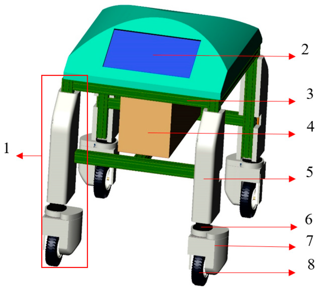
2.1. Design Scheme and Working Principle of Self-Balancing Mobile Robot in Greenhouse
2.2. Research on Control Method of Body Attitude Angle
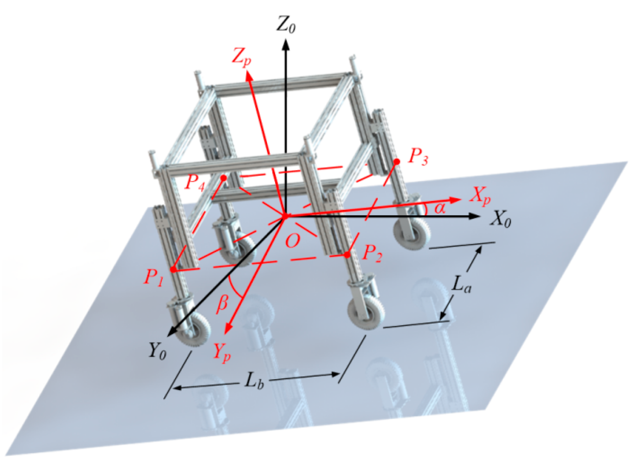
2.2.1. Attitude Angle Control Model Establishment
2.2.2. Adjusting Speed Control Model
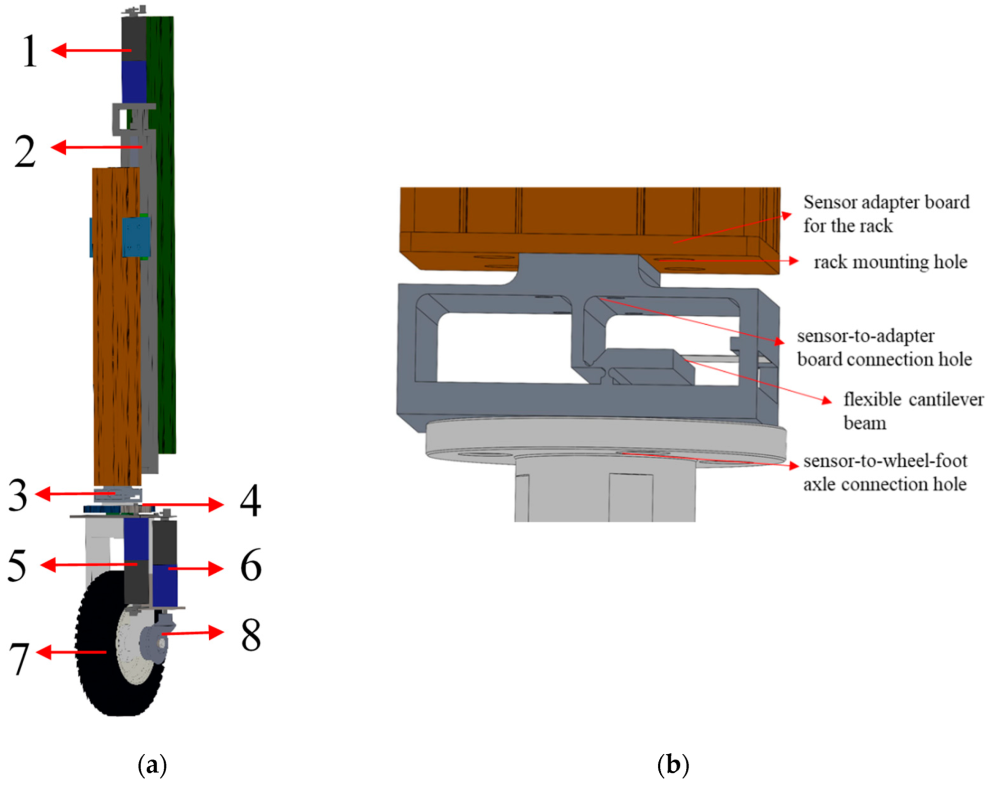
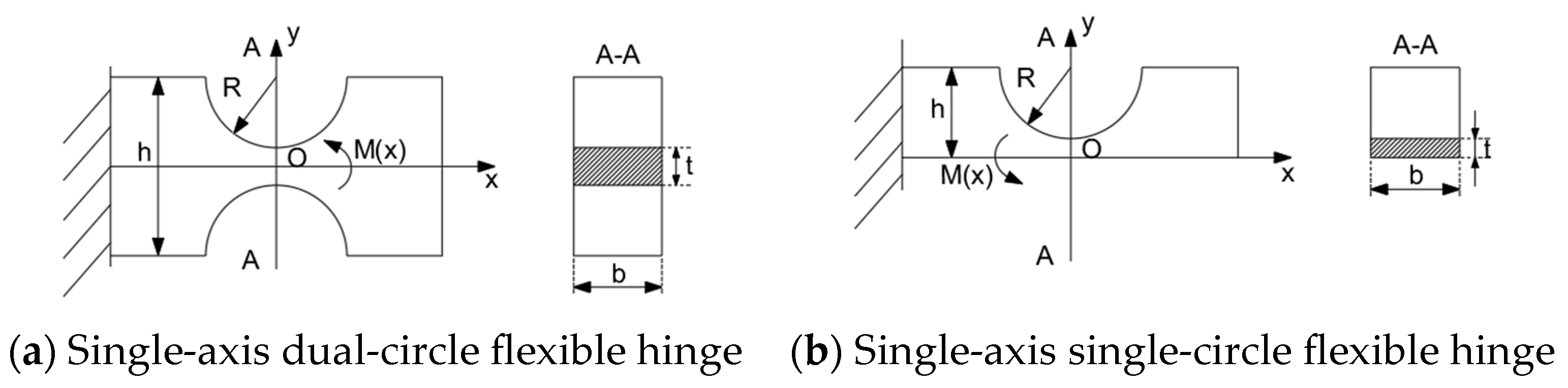
2.3. The Design of PR Flexible Joint Sensor
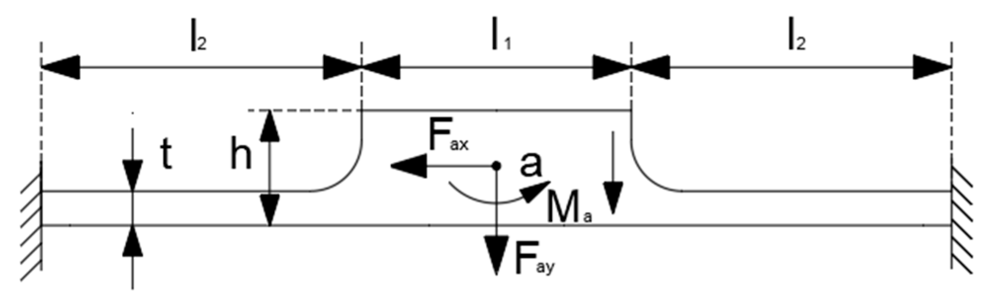
2.3.1. Constraint Analysis of Flexible Joint Sensor
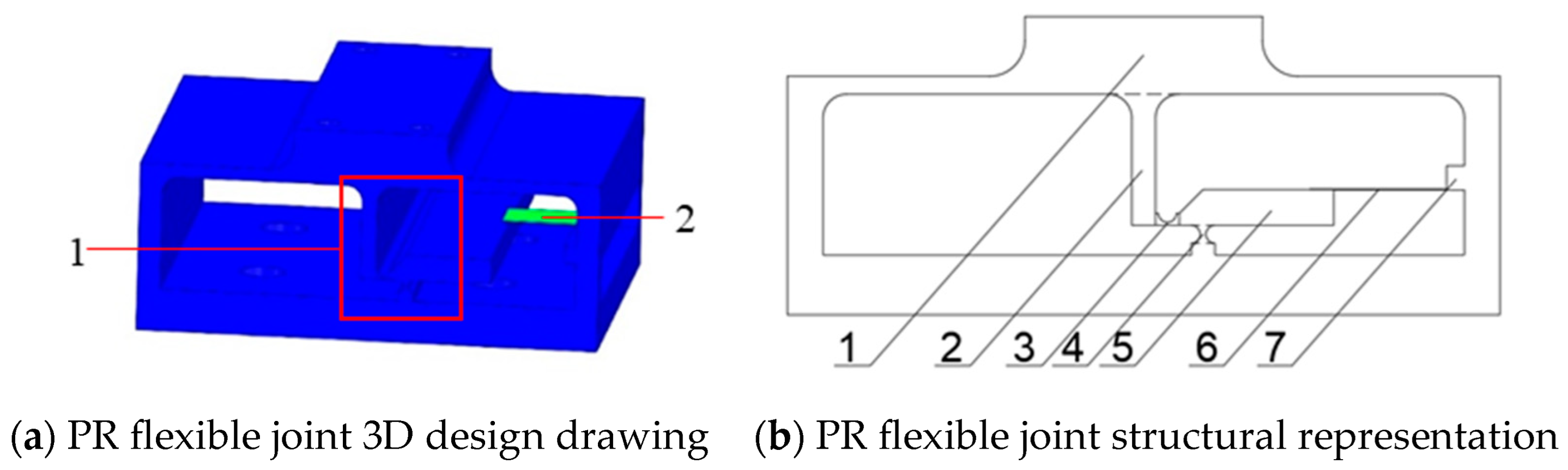
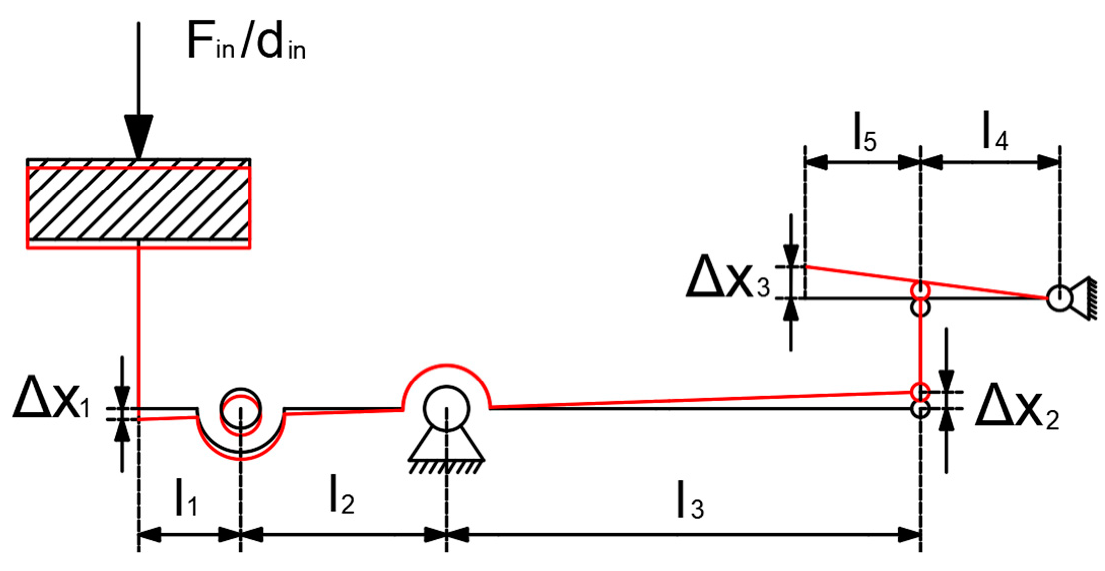
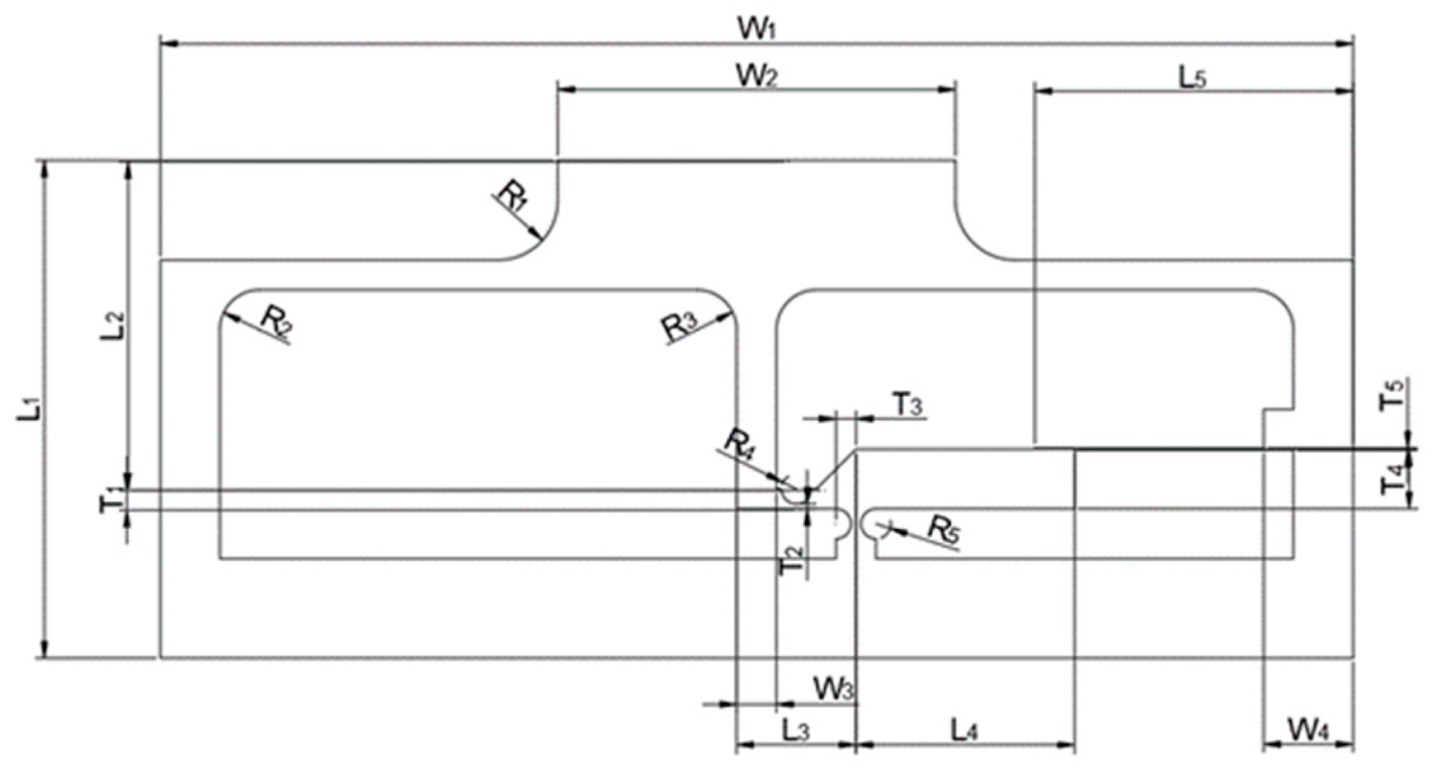
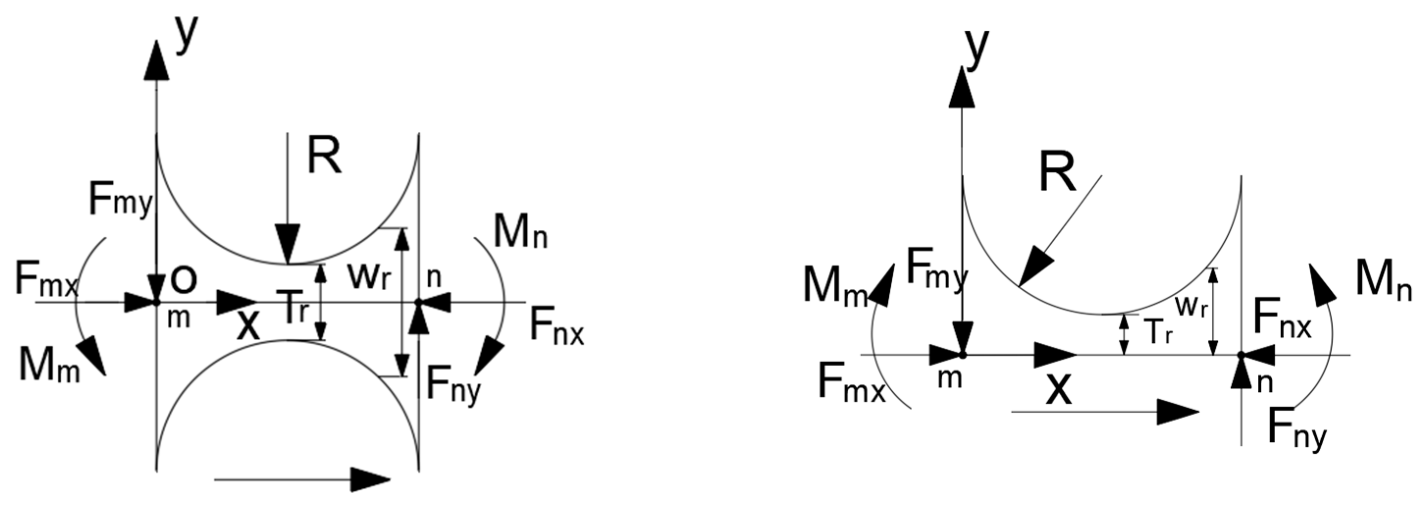
2.3.2. PR-Type Displacement Transfer Amplification Structure Design
2.3.3. Solution of PR-Type Flexible Joint Magnification
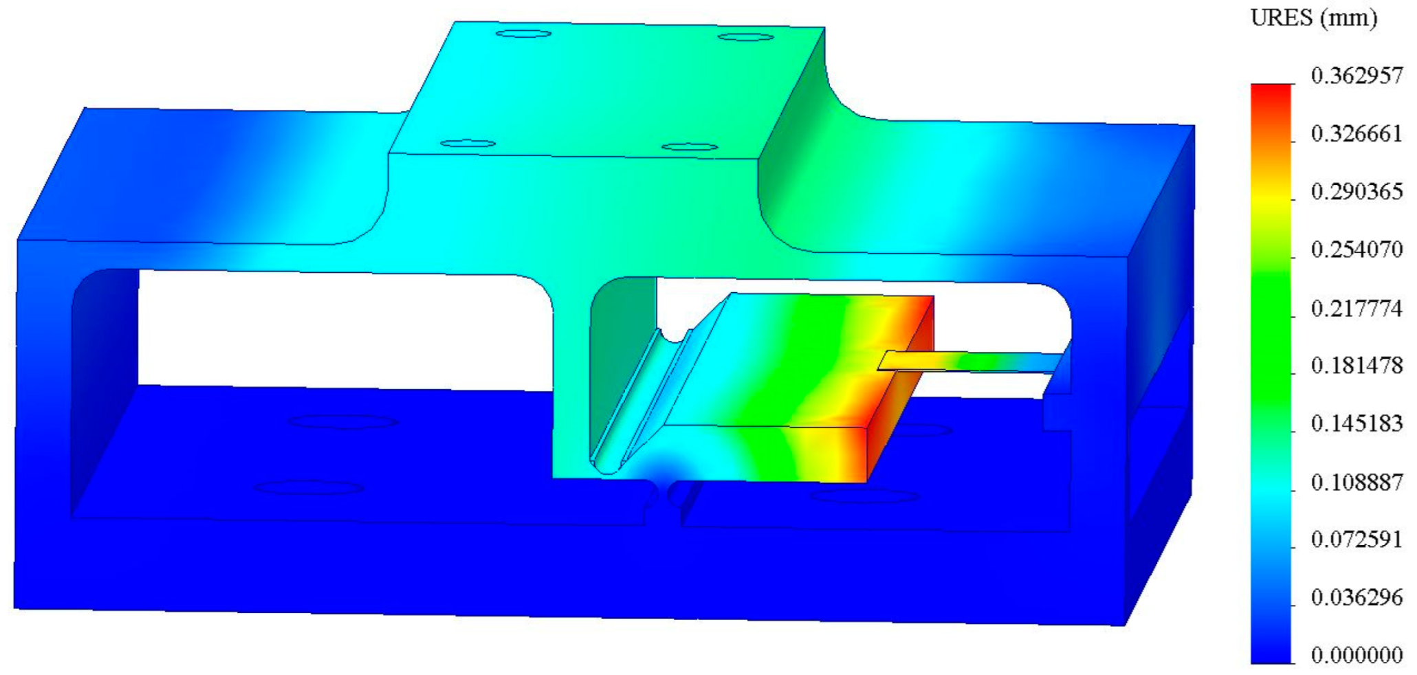
2.4. Finite Element Simulation Analysis of Flexible Joints
2.4.1. Stiffness Finite Element Analysis of Flexible Joint Sensor
- (1)
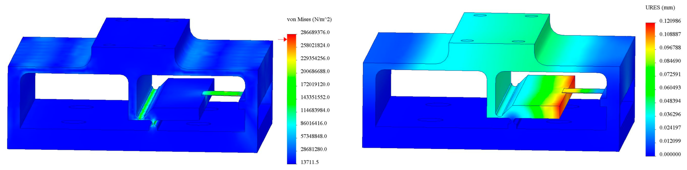
- Define the material properties of the structure according to the material parameters in the table. Then, fix the flexible joint with constraints and select the contact surface between the end of the lever-type micro-displacement amplification structure and the flexible cantilever beam as non-penetrating and the global contact as bonded. During operation, the flexible joint is subjected to a surface force that is uniformly distributed; therefore, a uniformly distributed surface force is applied at the input end with four spans.
- (2)
- Obtain the simulation results and, based on the relationship between the input force Fin, output displacement Dout, and stiffness k, as shown in Equation (A41) (Appendix A), obtain the stiffness of the flexible joint.
2.4.2. Finite Element Analysis of Effective Magnification Model of PR Flexible Joint
- (1)
- Define the material properties of the structure according to the material parameters in the table. Then, fix the flexible joint with constraints and select the contact surface between the end of the lever-type micro-displacement amplification structure and the flexible cantilever beam as non-penetrating and the global contact as bonded. During operation, the flexible joint is subjected to a uniformly distributed surface force with an area of 1172 mm2; therefore, different displacements of 5 μm, 10 μm, 20 μm, and 50 μm can be directly input to the surface to obtain the corresponding output displacement.
- (2)
3. Results and Discussion
3.1. Design of Performance Testing Experiments
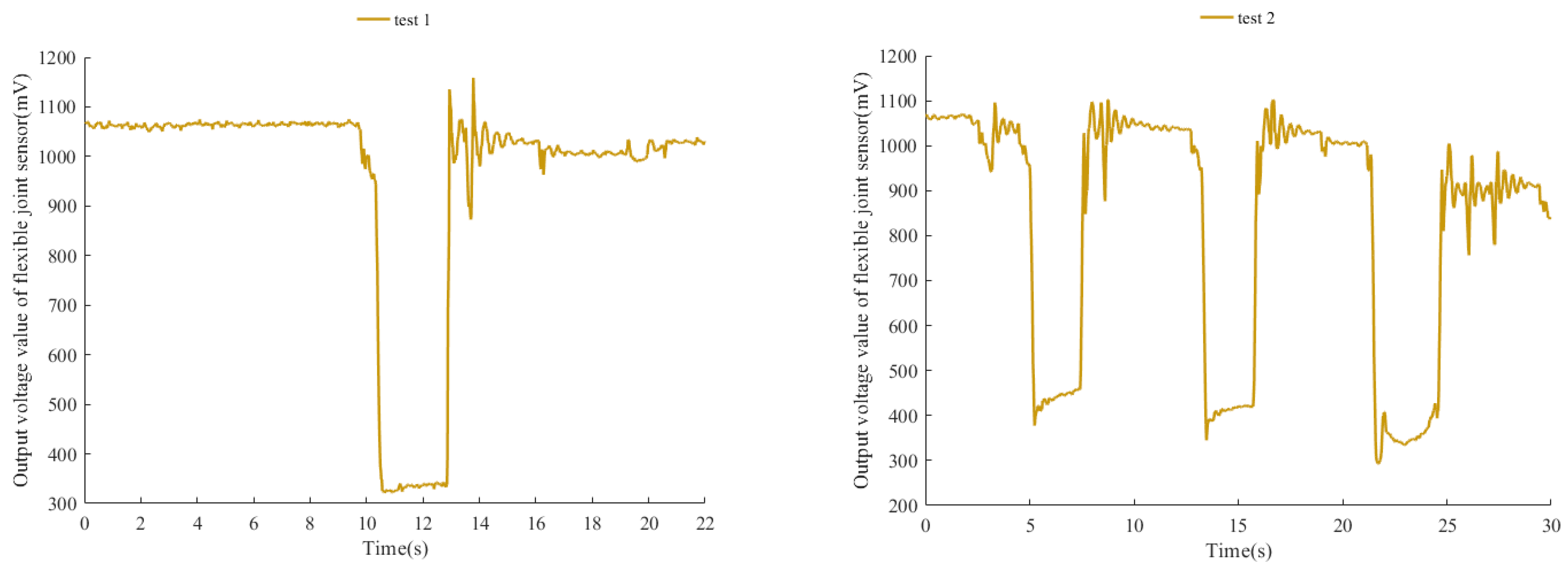
3.1.1. Performance Test Plan of PR Flexible Joint Sensor
- (1)
- The first set of test cycles was set to 22 s, with an initial state of grounding and holding for 10 s, then transitioning to a suspended state and holding for 2 s, and finally transitioning back to the grounding state and holding for 10 s.
- (2)
- The second set of test cycles was set to 30 s, with an initial state of grounding and holding for 5.5 s, then transitioning to a suspended state and holding for 2.5 s, alternating between the grounding and suspended states twice, and finally transitioning back to the grounding state and holding for 6 s.
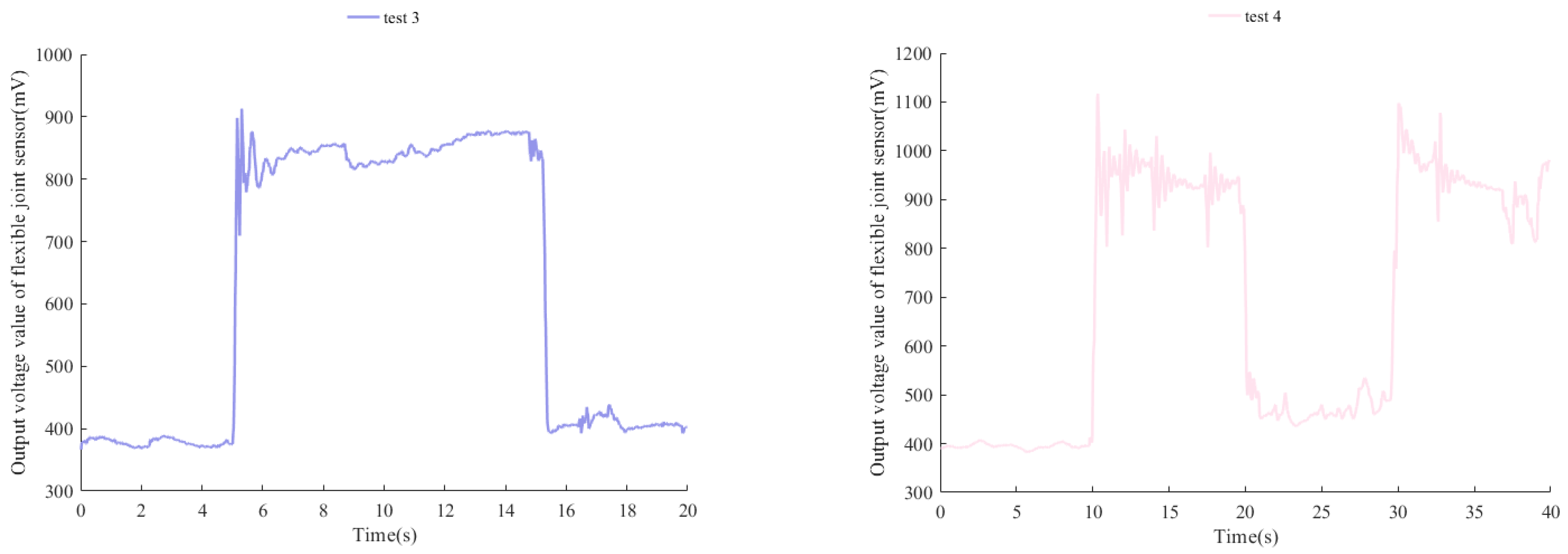
- (3)
- The third set of test cycles was set to 20 s, with an initial state of suspension and holding for 5 s, then transitioning to the grounding state and holding for 10 s, and finally transitioning back to the suspended state and holding for 5 s.
- (4)
- The fourth set of test cycles was set to 40 s, with an initial state of suspension and holding for 10 s, then transitioning to the grounding state and holding for 10 s, alternating between the suspension and grounding states once, and finally transitioning back to the suspension state and holding for 10 s.
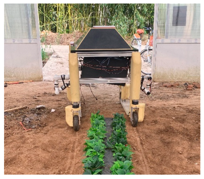
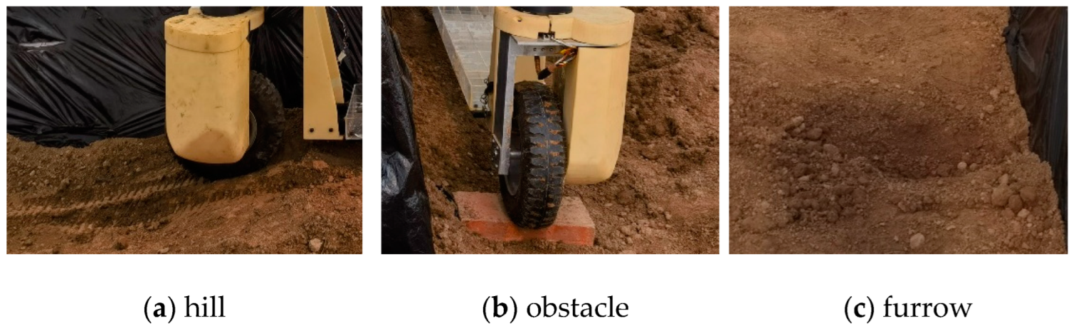
3.1.2. Field Test Plan for Self-Balancing System of Mobile Robots in Greenhouse
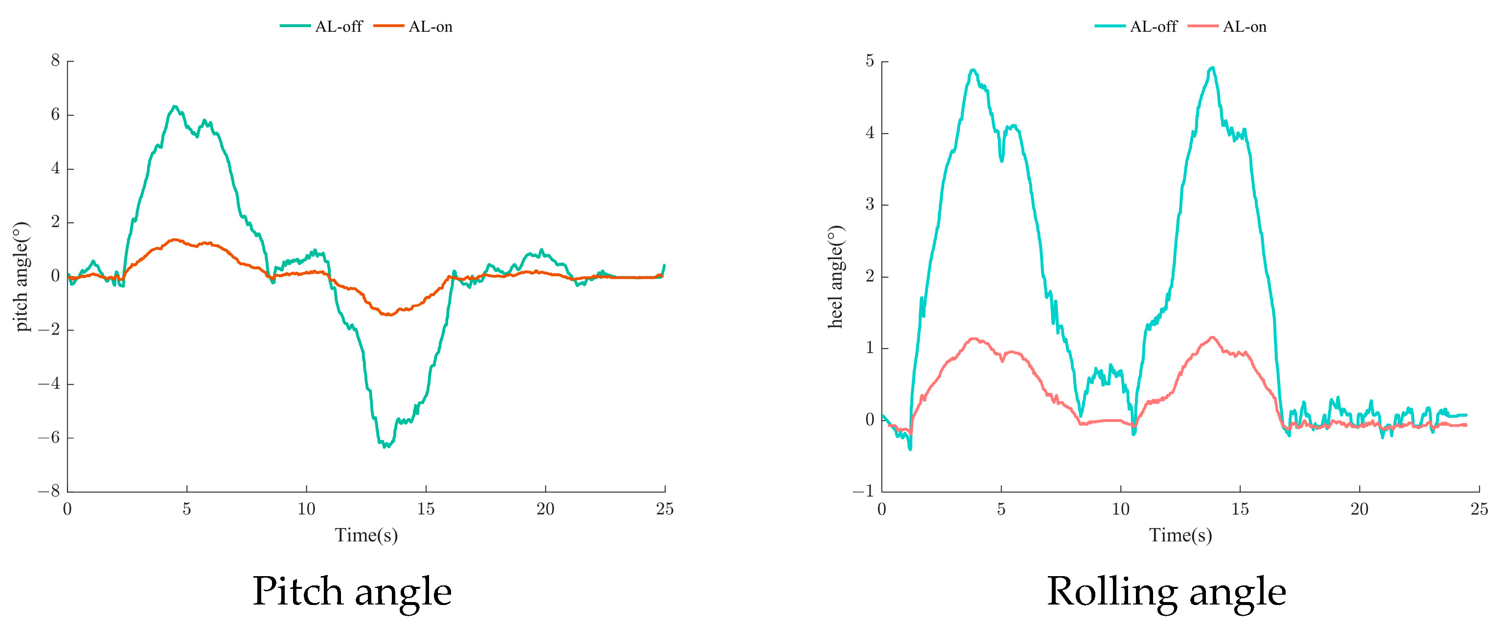
- (a)
- The environment of climbing a hill
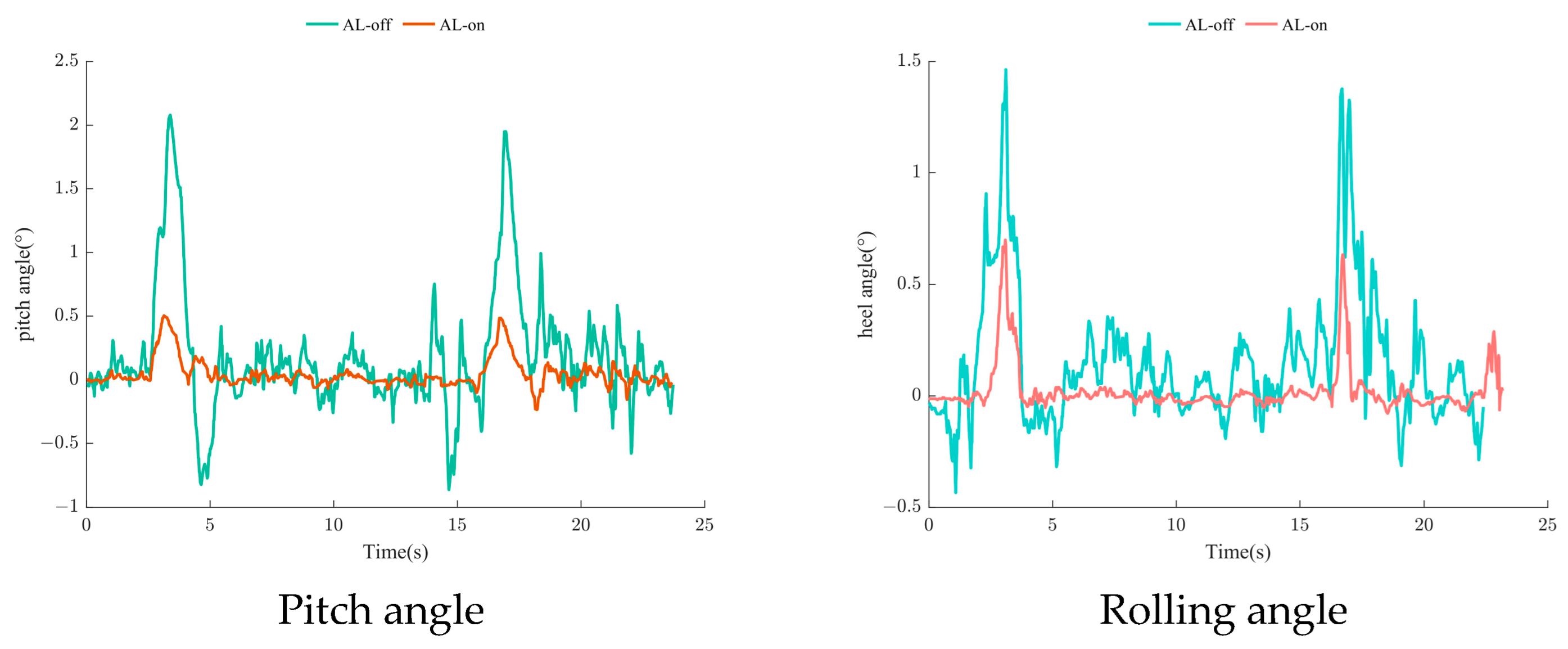
- (b)
- The environment of traversing obstacles
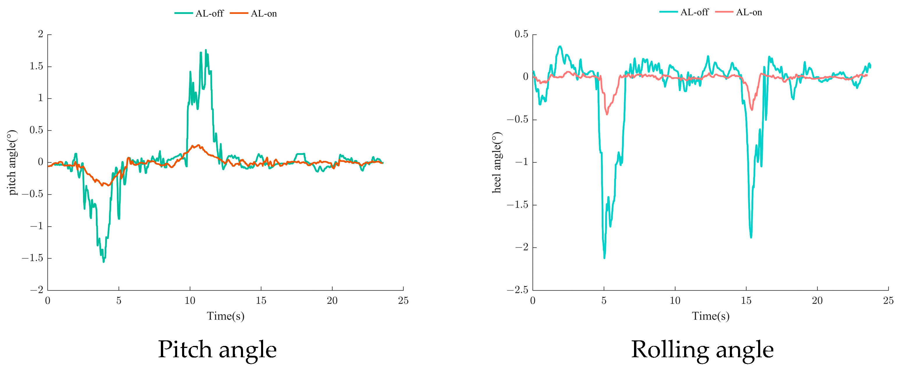
- (c)
- The environment of crossing a furrow
3.2. Mobile Platform Robot Performance Test Results and Analysis
3.2.1. Performance Test Results and Analysis of PR Flexible Joint Sensor
3.2.2. Field Performance Test Results and Analysis of the Greenhouse Mobile Robot Self-Balancing System
4. Conclusions
Author Contributions
Funding
Institutional Review Board Statement
Data Availability Statement
Conflicts of Interest
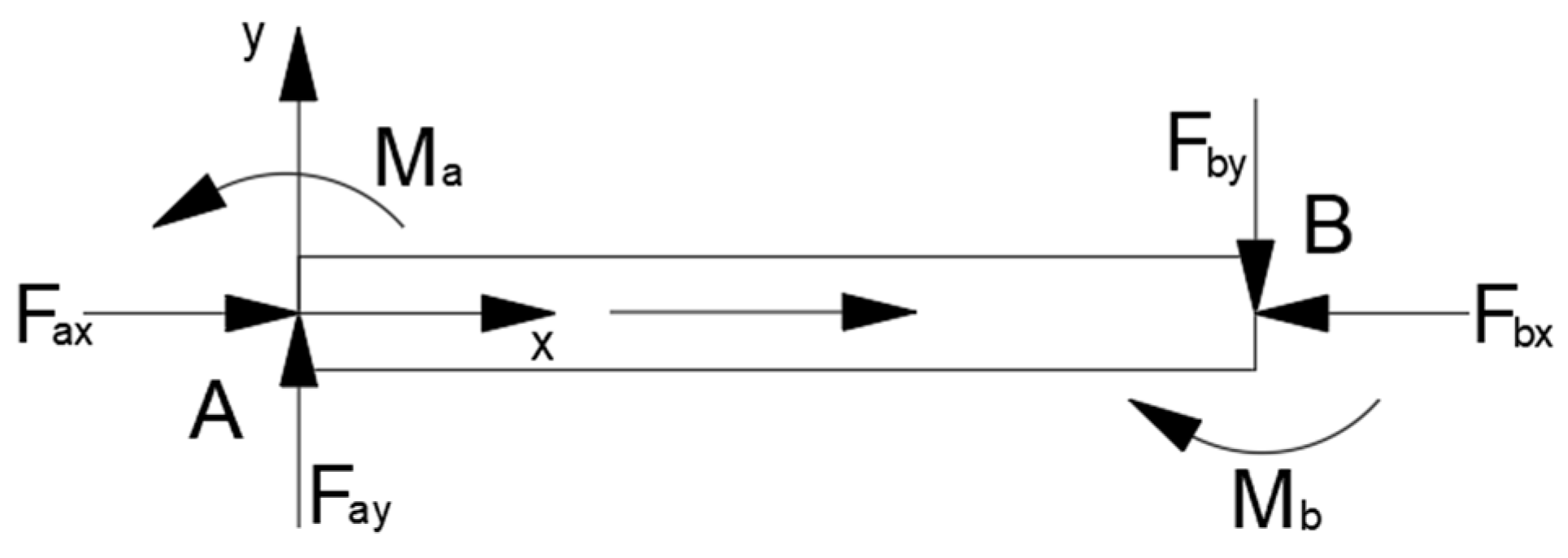
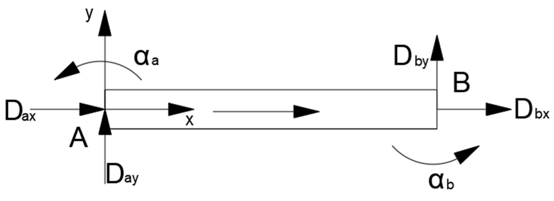
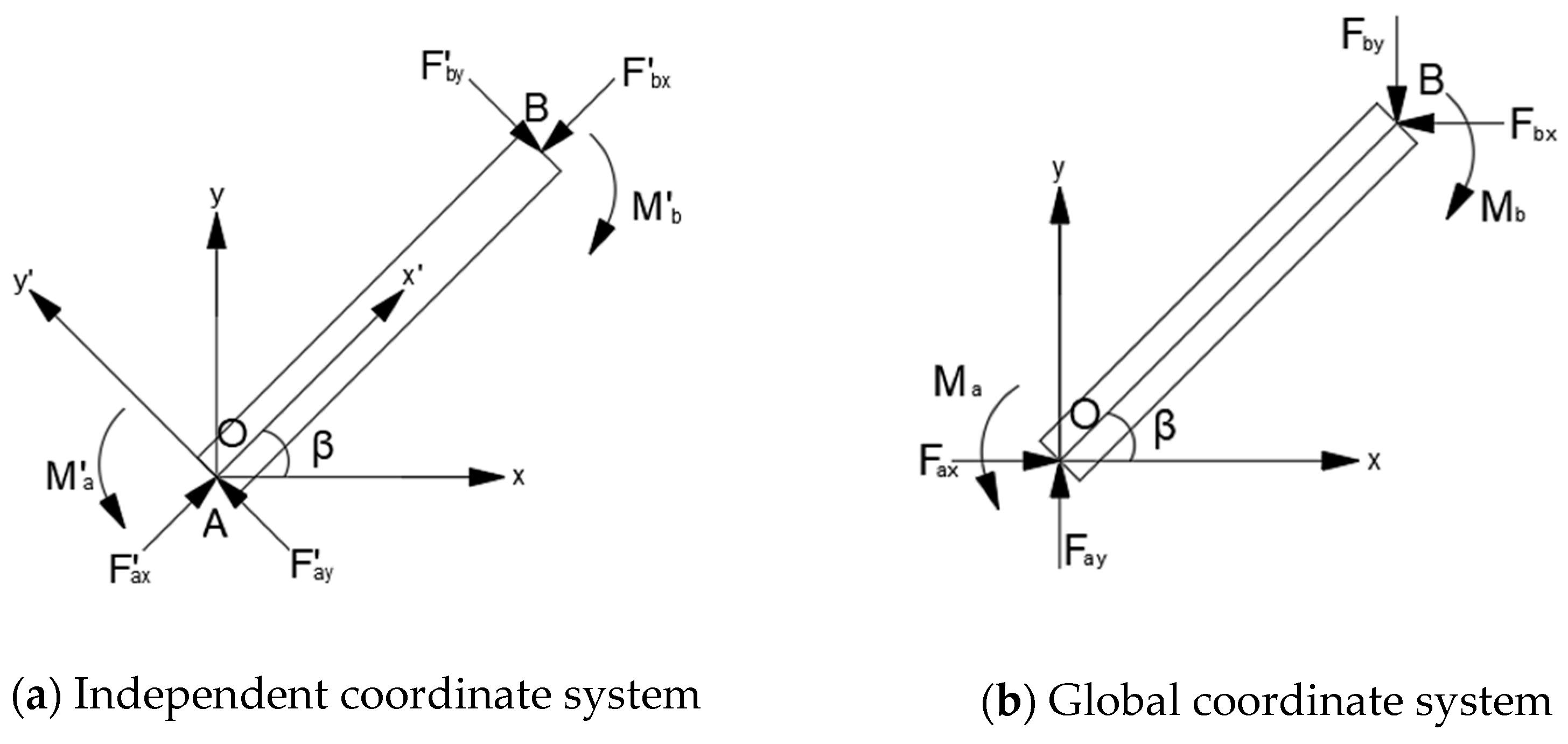
Appendix A
- (1)
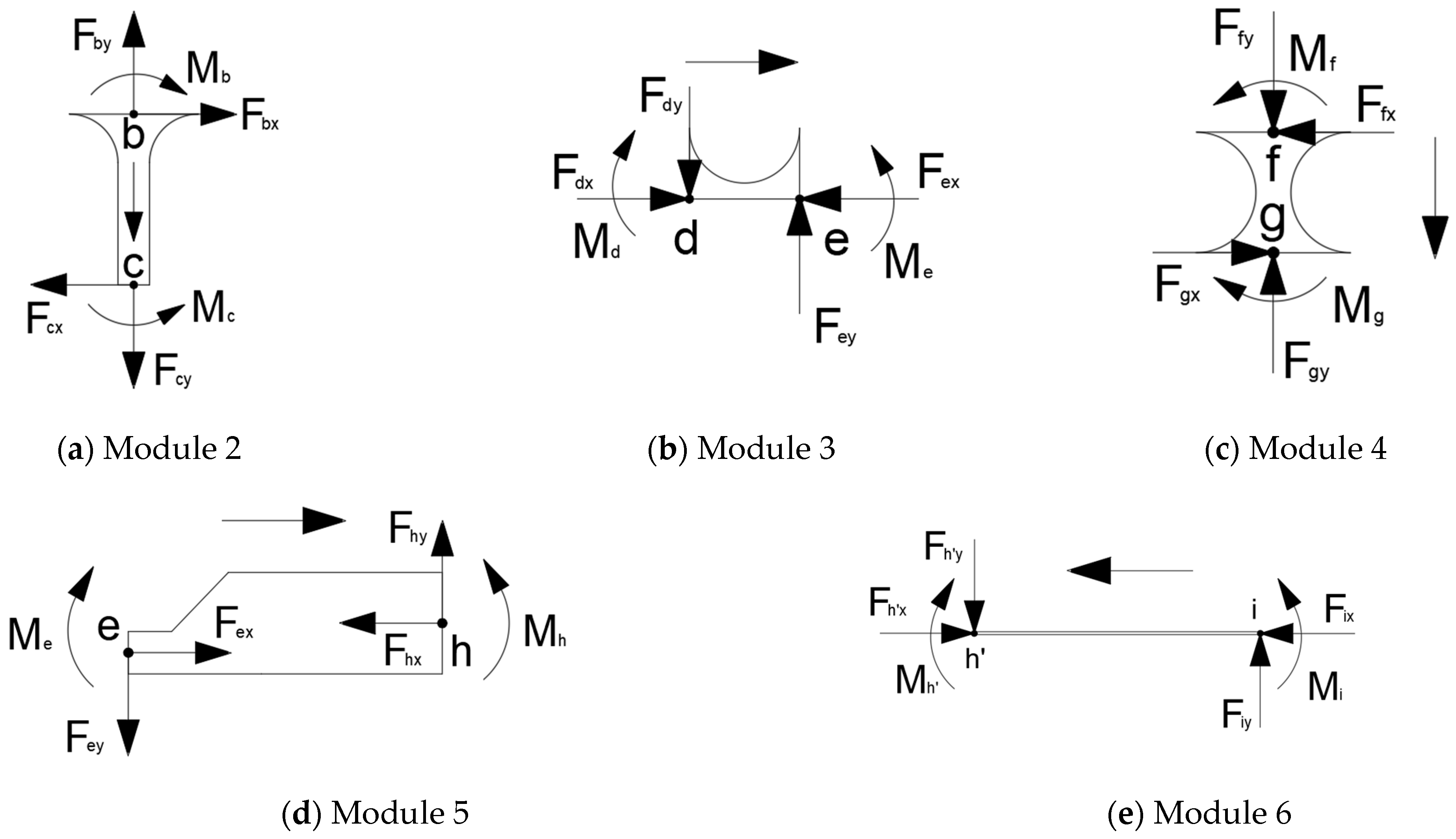
- Transfer matrix calculation method


- (2)
- Stiffness solution of flexible guide pair module

- (3)
- Solution of transfer matrix of flexible hinge module

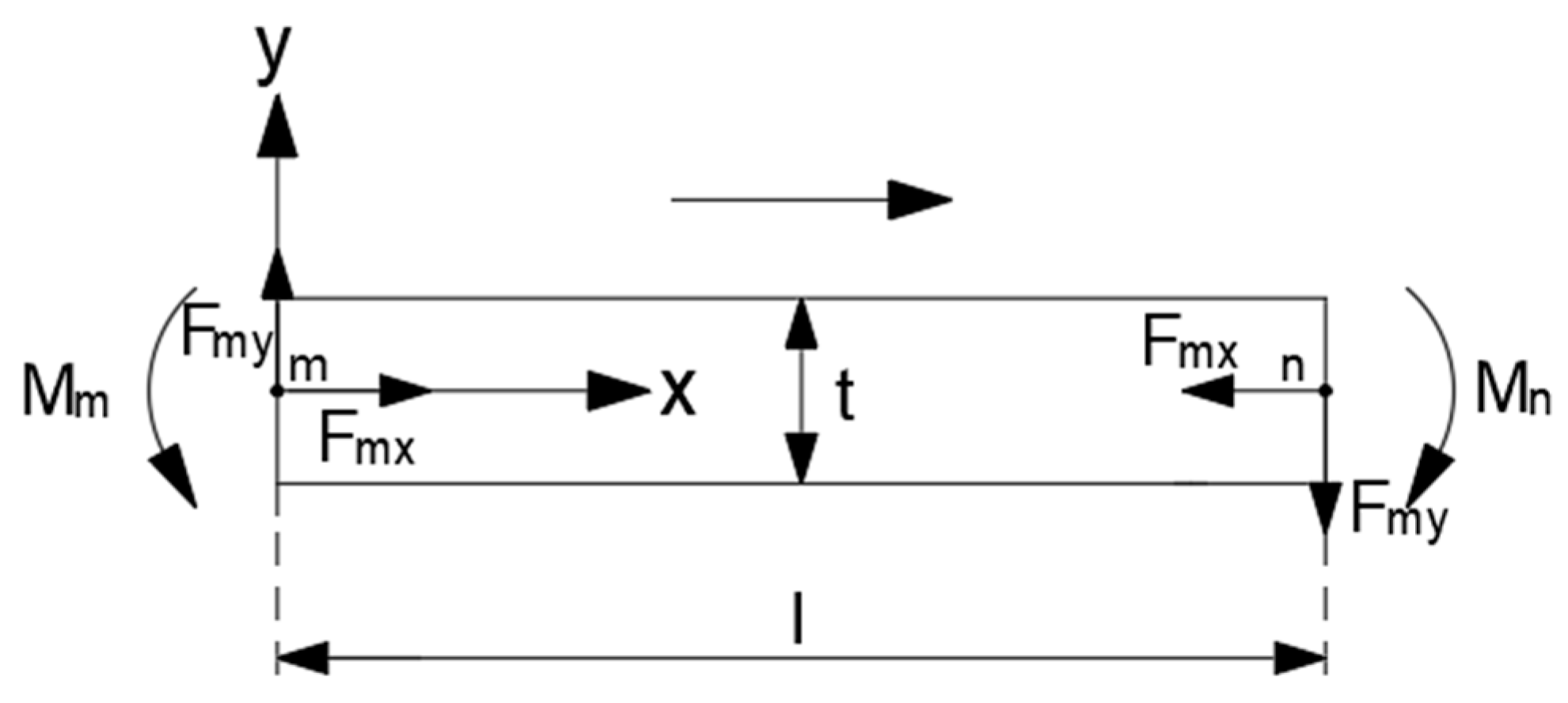
- (4)
- Solution of transfer matrix of flexible beam module


References
- Yu, Y.; Zhang, K.; Liu, H.; Yang, L.; Zhang, D. Real-Time Visual Localization of the Picking Points for a Ridge-Planting Strawberry Harvesting Robot. IEEE Access 2020, 8, 116556–116568. [Google Scholar] [CrossRef]
- Yu, Y.; Zhang, K.; Yang, L.; Zhang, D. Fruit detection for strawberry harvesting robot in non-structural environment based on Mask-RCNN. Comput. Electron. Agric. 2019, 163, 104846. [Google Scholar] [CrossRef]
- Bechar, A.; Vigneault, C. Agricultural robots for field operations: Concepts and components. Biosyst. Eng. 2016, 149, 94–111. [Google Scholar] [CrossRef]
- Gao, C.; He, L.; Fang, W.; Wu, Z.; Jiang, H.; Li, R.; Fu, L. A novel pollination robot for kiwifruit flower based on preferential flowers selection and precisely target. Comput. Electron. Agric. 2023, 207, 107762. [Google Scholar] [CrossRef]
- Peng, C.; Vougioukas, S.G. Deterministic predictive dynamic scheduling for crop-transport co-robots acting as harvesting aids. Comput. Electron. Agric. 2020, 178, 105702. [Google Scholar] [CrossRef]
- Wang, X.; Kang, H.; Zhou, H.; Au, W.; Wang, M.Y.; Chen, C. Development and evaluation of a robust soft robotic gripper for apple harvesting. Comput. Electron. Agric. 2023, 204, 107552. [Google Scholar] [CrossRef]
- Suzumura, A.; Fujimoto, Y. Real-Time Motion Generation and Control Systems for High Wheel-Legged Robot Mobility. IEEE Trans. Ind. Electron. 2013, 61, 3648–3659. [Google Scholar] [CrossRef]
- Xu, K.; Wang, S.; Yue, B.; Wang, J.; Peng, H.; Liu, D.; Chen, Z.; Shi, M. Adaptive impedance control with variable target stiffness for wheel-legged robot on complex unknown terrain. Mechatronics 2020, 69, 102388. [Google Scholar] [CrossRef]
- Shrivastava, S.; Karsai, A.; Aydin, Y.O.; Pettinger, R.; Bluethmann, W.; Ambrose, R.O.; Goldman, D.I. Material remodeling and unconventional gaits facilitate locomotion of a robophysical rover over granular terrain. Sci. Robot. 2020, 5, eaba3499. [Google Scholar] [CrossRef]
- Sun, Z.; Hu, S.; Xie, H.; Li, H.; Zheng, J.; Chen, B. Fuzzy adaptive recursive terminal sliding mode control for an agricultural omnidirectional mobile robot. Comput. Electr. Eng. 2023, 105, 108529. [Google Scholar] [CrossRef]
- Fan, G.; Wang, Y.; Zhang, X.; Zhao, J.; Song, Y. Design and experiment of automatic leveling control system for orchards lifting platform. Trans. Chin. Soc. Agric. Eng. 2017, 33, 38–46. [Google Scholar] [CrossRef]
- Chen, L.; Karkee, M.; He, L.; Wei, Y.; Zhang, Q. Evaluation of a Leveling System for a Weeding Robot under Field Condition. IFAC-PapersOnLine 2018, 51, 368–373. [Google Scholar] [CrossRef]
- Iagnemma, K.; Rzepniewski, A.; Dubowsky, S.; Schenker, P. Control of Robotic Vehicles with Actively Articulated Suspensions in Rough Terrain. Auton. Robot. 2003, 14, 5–16. [Google Scholar] [CrossRef]
- Grand, C.; Benamar, F.; Plumet, F. Motion kinematics analysis of wheeled–legged rover over 3D surface with posture adaptation. Mech. Mach. Theory 2010, 45, 477–495. [Google Scholar] [CrossRef]
- Lim, K.B.; Yoon, Y. Reconfiguration Planning for a Robotic Vehicle with Actively Articulated Suspension in Obstacle Terrain during Straight Motion. Adv. Robot. 2012, 26, 1471–1494. [Google Scholar] [CrossRef]
- Reid, W.; Perez-Grau, F.J.; Goktogan, A.H.; Sukkarieh, S. Actively articulated suspension for a wheel-on-leg rover operating on a Martian analog surface. In Proceedings of the 2016 IEEE International Conference on Robotics and Automation, Stockholm, Sweden, 16–21 May 2016. [Google Scholar]
- Qi, W.; Li, Y.; Zhang, J.; Qin, C.; Liu, C.; Yin, Y. Double Closed Loop Fuzzy PID Control Method of Tractor Body Leveling on Hilly and Mountainous Areas. Trans. Chin. Soc. Agric. Mach. 2019, 50, 17–23. [Google Scholar]
- Yin, X.; An, J.; Wang, Y.; Li, J.; Jin, C. Design and Test of Automatic Beam Leveling System for High-clearance Sprayer. Trans. Chin. Soc. Agric. Mach. 2022, 53, 98–105. [Google Scholar] [CrossRef]
- Cordes, F.; Kirchner, F.; Babu, A. Design and field testing of a rover with an actively articulated suspension system in a Mars analog terrain. J. Field Robot. 2018, 35, 1149–1181. [Google Scholar] [CrossRef]
- Sun, Y.; He, J.; Xing, Y. Multi-target coordinated control of wheel-legged Mars rover. Acta Aeronaut. Astronaut. Sin. 2021, 42, 327–339. [Google Scholar] [CrossRef]
- Shu, Y.; Zhuang, W.; Li, K.; Yang, M. Weak leg compensation strategy and electromechanical joint simulation for a four-leg electromechanical leveling system. Radar ECM 2017, 37, 55–59. [Google Scholar] [CrossRef]
- Dai, J.; Chen, C.-Y.; Zhu, R.; Yang, G.; Wang, C.; Bai, S. Suppress Vibration on Robotic Polishing with Impedance Matching. Actuators 2021, 10, 59. [Google Scholar] [CrossRef]
- Savaee, E.; Hanzaki, A.R.; Anabestani, Y. Kinematic Analysis and Odometry-Based Navigation of an Omnidirectional Wheeled Mobile Robot on Uneven Surfaces. J. Intell. Robot. Syst. 2023, 108, 13. [Google Scholar] [CrossRef]
- Terakawa, T.; Komori, M.; Matsuda, K.; Mikami, S. A Novel Omnidirectional Mobile Robot with Wheels Connected by Passive Sliding Joints. IEEE/ASME Trans. Mechatron. 2018, 23, 1716–1727. [Google Scholar] [CrossRef]
- Hernandez-Barragan, J.; Martinez-Soltero, G.; Rios, J.D.; Lopez-Franco, C.; Alanis, A.Y. A Metaheuristic Optimization Approach to Solve Inverse Kinematics of Mobile Dual-Arm Robots. Mathematics 2022, 10, 4135. [Google Scholar] [CrossRef]
- Leng, J.; Mou, H.; Tang, J.; Li, Q.; Zhang, J. Design, Modeling, and Control of a New Multi-Motion Mobile Robot Based on Spoked Mecanum Wheels. Biomimetics 2023, 8, 183. [Google Scholar] [CrossRef] [PubMed]
- Wang, H.; Xu, Z.; Zhou, H. Design of heavy load vehicle leveling systems based on CANopen. J. China Univ. Metrol. 2018, 29, 269–275. [Google Scholar]
- Ha, J.-L.; Kung, Y.-S.; Hu, S.-C.; Fung, R.-F. Optimal design of a micro-positioning Scott-Russell mechanism by Taguchi method. Sens. Actuators A Phys. 2006, 125, 565–572. [Google Scholar] [CrossRef]
- Liu, G.; He, Z.; Bai, G.; Zheng, J.; Zhou, J.; Chang, M. Modeling and Experimental Study of Double-Row Bow-Type Micro-Displacement Amplifier for Direct-Drive Servo Valves. Micromachines 2020, 11, 312. [Google Scholar] [CrossRef]
- Wu, H.; Lai, L.; Zhang, L.; Zhu, L. A novel compliant XY micro-positioning stage using bridge-type displacement amplifier embedded with Scott-Russell mechanism. Precis. Eng. 2022, 73, 284–295. [Google Scholar] [CrossRef]
- Ling, M.; Zhang, C.; Chen, L. Optimized design of a compact multi-stage displacement amplification mechanism with enhanced efficiency. Precis. Eng. 2022, 77, 77–89. [Google Scholar] [CrossRef]
- Elsisy, M.M.; Arafa, M.H.; Saleh, C.A.; Anis, Y.H. Modeling of a Symmetric Five-Bar Displacement Amplification Compliant Mechanism for Energy Harvesting. Sensors 2021, 21, 1095. [Google Scholar] [CrossRef] [PubMed]
- Hui, L.X.; Lei, G.; Yan, W.; Haoran, S.; Yong, H. Micro-displacement amplifier of giant magnetostrictive actuator using flexure hinges. J. Magn. Magn. Mater. 2022, 556, 169415. [Google Scholar] [CrossRef]
- Fan, W.; Jin, H.; Fu, Y.; Lin, Y. A type of symmetrical differential lever displacement amplification mechanism. Mech. Ind. 2021, 22, 5. [Google Scholar] [CrossRef]


| Material | Parameters | |||
|---|---|---|---|---|
| Elastic Modulus E (GPa) | Poisson’s Ratio ν | Yield Strength σ (MPa) | Density ρ | |
| 6061-T6 aluminum alloy (main part) | 68.9 | 0.33 | 275 | 2700 |
| 65 Mn (signal output structure) | 206 | 0.3 | 78.4 | 7.85 |
| Parameters | Length/mm | Parameters | Length/mm |
|---|---|---|---|
| L1 | 25 | R1 | 2 |
| L2 | 16.5 | R2 | 2 |
| L3 | 5 | R3 | 2 |
| L4 | 11 | R4 | 0.75 |
| L5 | 16 | R5 | 0.75 |
| T1 | 1 | W1 | 60 |
| T2 | 0.25 | W2 | 20 |
| T3 | 0.5 | W3 | 2 |
| T4 | 3 | W4 | 4.5 |
| T5 | 0.1 | Joint width | 60 |
| Input Force Fin/N | Output Displacement Dout/μm | Stiffness k/(N/μm) | Relative Error (%) | |
|---|---|---|---|---|
| Simulation Stiffness | Theoretical Stiffness | |||
| 100 | 21.52 | 4.6468 | 5.0065 | 7.74 |
| 300 | 64.57 | 4.6461 | 5.0118 | 7.87 |
| 500 | 107.6 | 4.6468 | 5.0098 | 7.81 |
| 900 | 193.7 | 4.6464 | 5.0148 | 7.93 |
| Input Displacement Din (μm) | Output Displacement Dout/μm | Magnification | Relative Error (%) | |
|---|---|---|---|---|
| Simulation Stiffness | Theoretical Stiffness | |||
| 5 | 17.65 | 3.51 | 3.20 | 9.69 |
| 10 | 35.30 | 3.53 | 3.30 | 6.97 |
| 20 | 70.59 | 3.53 | 3.56 | 1.40 |
| 50 | 176.48 | 3.53 | 3.60 | 1.94 |
| Operational Mode | Response Time (s) | Average Response Time (s) |
|---|---|---|
| suspension-grounding | 0.11 | 0.16 |
| 0.16 | ||
| 0.21 | ||
| 0.15 | ||
| 0.18 | ||
| grounding-suspension | 0.14 | 0.12 |
| 0.09 | ||
| 0.10 | ||
| 0.14 | ||
| 0.13 |
| Hill Climbing Test | Extremal Value | Mean Value | Standard Deviation | |||
|---|---|---|---|---|---|---|
| Pitch Angle | Rolling Angle | Pitch Angle | Rolling Angle | Pitch Angle | Rolling Angle | |
| AL-off | 6.39 | 4.92 | 1.87 | 1.65 | 2.14 | 1.71 |
| AL-on | 1.42 | 1.22 | 0.41 | 0.40 | 0.47 | 0.43 |
| reduce ratio | 77.78% | 75.20% | 78.07% | 75.76% | 78.04% | 74.85% |
| Traversing Obstacle Test | Extremal Value | Mean Value | Standard Deviation | |||
|---|---|---|---|---|---|---|
| Pitch Angle | Rolling Angle | Pitch Angle | Rolling Angle | Pitch Angle | Rolling Angle | |
| AL-off | 2.09 | 1.51 | 0.30 | 0.21 | 0.41 | 0.26 |
| AL-on | 0.53 | 0.71 | 0.08 | 0.04 | 0.10 | 0.10 |
| reduce ratio | 74.64% | 52.98% | 73.33% | 80.95% | 75.61% | 61.54% |
| Crossing Furrow Test | Extremal Value | Mean Value | Standard Deviation | |||
|---|---|---|---|---|---|---|
| Pitch Angle | Rolling Angle | Pitch Angle | Rolling Angle | Pitch Angle | Rolling Angle | |
| AL-off | 1.79 | 2.15 | 0.24 | 0.24 | 0.40 | 0.40 |
| AL-on | 0.35 | 0.44 | 0.08 | 0.04 | 0.09 | 0.07 |
| reduce ratio | 80.45% | 79.53% | 66.67% | 83.33% | 77.5% | 82.5% |
Disclaimer/Publisher’s Note: The statements, opinions and data contained in all publications are solely those of the individual author(s) and contributor(s) and not of MDPI and/or the editor(s). MDPI and/or the editor(s) disclaim responsibility for any injury to people or property resulting from any ideas, methods, instructions or products referred to in the content. |
© 2023 by the authors. Licensee MDPI, Basel, Switzerland. This article is an open access article distributed under the terms and conditions of the Creative Commons Attribution (CC BY) license (https://creativecommons.org/licenses/by/4.0/).
Share and Cite
Zhang, Y.; Song, Y.; Lu, F.; Zhang, D.; Yang, L.; Cui, T.; He, X.; Zhang, K. Design and Experiment of Greenhouse Self-Balancing Mobile Robot Based on PR Joint Sensor. Agriculture 2023, 13, 2040. https://doi.org/10.3390/agriculture13102040
Zhang Y, Song Y, Lu F, Zhang D, Yang L, Cui T, He X, Zhang K. Design and Experiment of Greenhouse Self-Balancing Mobile Robot Based on PR Joint Sensor. Agriculture. 2023; 13(10):2040. https://doi.org/10.3390/agriculture13102040
Chicago/Turabian StyleZhang, Yaohui, Yugang Song, Fanggang Lu, Dongxing Zhang, Li Yang, Tao Cui, Xiantao He, and Kailiang Zhang. 2023. "Design and Experiment of Greenhouse Self-Balancing Mobile Robot Based on PR Joint Sensor" Agriculture 13, no. 10: 2040. https://doi.org/10.3390/agriculture13102040