Optimization and Accuracy Analysis of a Soil–Planter Model during the Sowing Period of Wheat after a Rice Stubble Based Discrete Element Method

Abstract

The soil during the sowing period of wheat after rice stubble cannot be accurately described by existing models and parameters with DEM because of its high moisture content and strong viscosity. The purpose of this study is to conduct an overall simulation of high-viscosity paddy soil and to analyze the accuracy of the model. Based on the results of an unconfined compression test and shear test, the range of bond parameters is preliminarily determined by a simulation test. Through the P-BD test and RSM test, the parameters with significant influence are determined to be normal stiffness per unit area (S_N), shear stiffness per unit area (S_S), and critical shear stress (C_S), and an optimized combination of these parameters is obtained. Based on the optimized model, the error range and error generation mechanism of the model are analyzed under different operating parameters. The results show that the optimal parameter combination is S_N of 1.07 × 10⁷ N/m³, S_S of 0.70 × 10⁷ N/m³, and C_S of 0.35 × 10⁵ Pa, corresponding to a compression force of 120.1 N and a shear force of 7.70 N. With an increase in forward speed or seeding quantity or a decrease in rotary plowing speed, the model accuracy tends to increase, and the range of relative errors was found to be from 8.8% to 28.4%. The results can provide a research basis for the study of the motion state of seeds under soil. It can also further enrich parameter data of soil discrete element simulation models and provide a reference for related research studies.

1. Introduction

The rice–wheat rotation system is an important method of wheat production in China and is commonly used in the middle and lower reaches of the Yangtze River plain [1,2]. The mainstream process of producing wheat under this model has changed due to alterations in the agricultural production model in China, i.e., rice harvesting–straw crushing and returning–wheat sowing–wheat harvesting [3,4]. The basic physical parameters of soils in this production mode differ significantly from those in other tillage systems. This is particularly evident because (i) under the rice–wheat rotation mode, the soil alternates between dry and wet periods, resulting in high soil compaction, hardening, and low porosity; (ii) the moisture content of rice plots are relatively high, and all straw is left on the field after rice harvesting, thus reducing field water evaporation efficiency. Hence, the soil has a high moisture content and strong viscosity [5,6]. 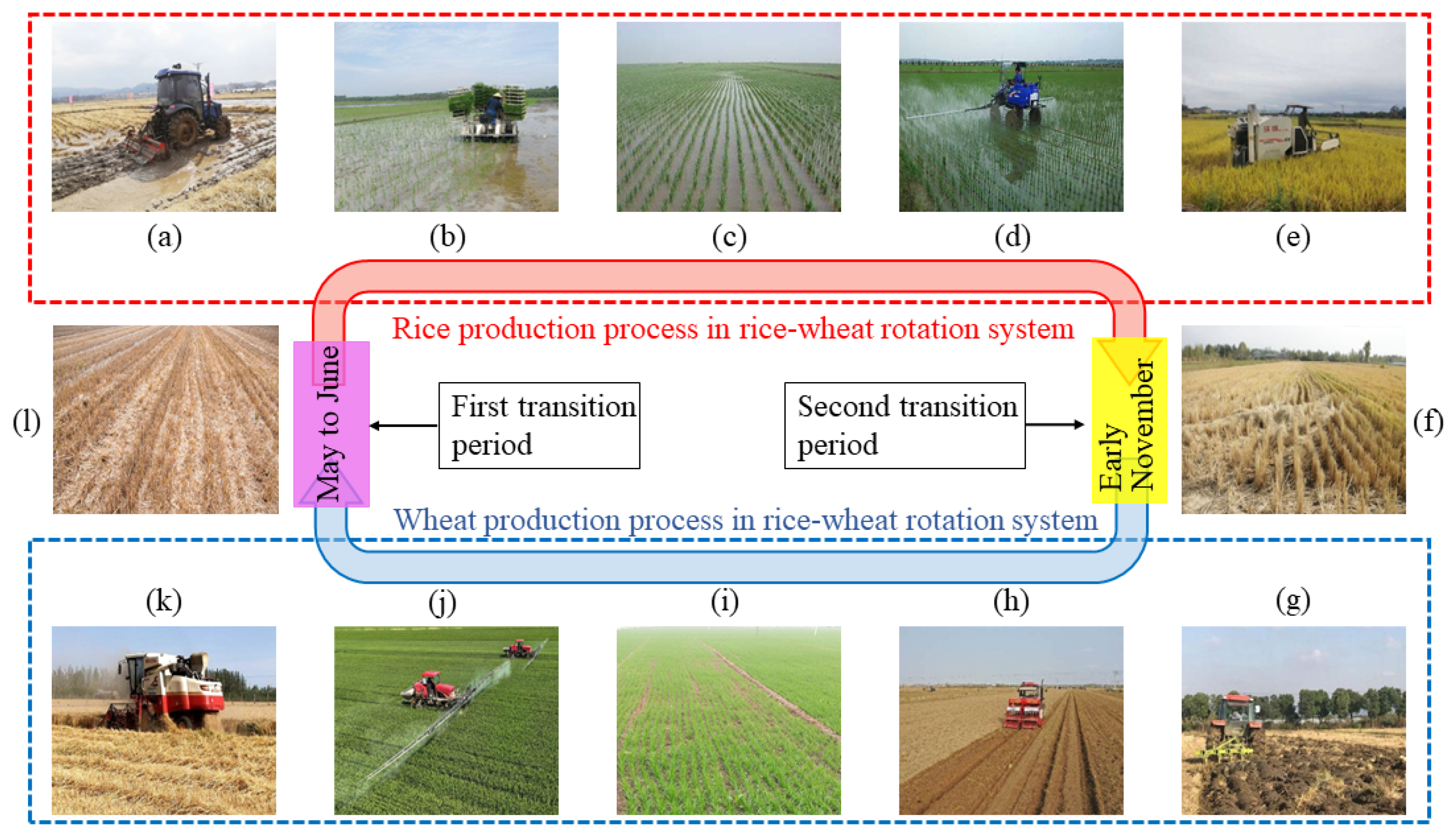Conventional wheat-sowing technology and equipment are not well adapted to the sowing conditions in the southern rice–wheat rotation area due to this unique cycle process (Figure 1) and significant differences in soil physical properties [7,8]. So, the development of wheat sowing equipment suitable for the agronomic model of the rice–wheat rotation system is an effective way to improve the mechanized sowing quality of wheat in full rice stubble fields.

Seeding performance for wheat planters is the result of collective seed–mechanical–soil action [9]. Seed location in the paddy soil is an important index to evaluate the performance of the wheat seeder; however, conventional tools cannot readily measure the state of seeds in soil [10]. Numerical simulation with DEM is an important visualization method for studying the seed–mechanical–soil interaction mechanism, which can effectively make up for the shortcomings of traditional measurement methods in the measurement of subsoil parameters [11,12,13,14].

Ucgul et al. determined appropriate DEM parameters for modeling soil–tool interactions in cohesionless soil using a linear plastic contact model and a natural slope angle test [15,16]. In addition, the discrete element parameters and the interaction process with the plow tools are simulated accurately by means of confined compression, direct shear tests, and simulating the actual working process [17,18,19]. Based on the Hertz–Mindlin (no slip) model, the material properties (cohesion, sliding friction angle, shear stress, internal friction angle) and soil–mechanism contact parameters of various soils, such as sandy soil [20], loess plateau slope soil [21], and loam soil [22], were measured and calibrated. These simulations served as a basis for analyzing soil interaction characteristics and implementation. The bonding model is mainly used to study compacted or agglomerated materials [23]. On the basis of soil parameters obtained by stacking angle, Li et al. investigated the crushing characteristics of agglomerate soil blocks using the shear test [24]; Ding et al. established a bond model of paddy field soil through uniaxial compression tests and conducted DEM analyses of subsoiling process in wet clay paddy soil [25]; Fang et al. analyzed the macroscopic and microscopic movement behaviors of soil, and the movement characteristics of straw, during rotary tillage process by comparing simulations and experiments [26,27]; Chen et al. established the DEM model of organic fertilizer composed of caked and bulk fertilizers, performed DEM simulations of solid fertilizer movement and breakage, and optimized the performance of solid organic fertilizer crushing and striping machine [28].

So far, the international research on the application of DEM for numerical simulation has mainly focused on the simulation of a stable mechanical state of materials, such as the parameter calibration of material particles in a stable state, the calibration of contact parameters between materials and equipment, and the movement characteristics of materials during motion [29]. However, there is a lack of research on using DEM to conduct an overall simulation of paddy soil before and after rotary tillage (modeling of soil dynamic mechanical properties). Moreover, few studies have explored the accuracy of DEM simulation under different operating parameters of seeders, as well as the variation pattern of simulation errors with operating parameters. Hence, the current study aimed to bridge this gap by calibrating the parameters of paddy soil (dynamic mechanical properties) before and after rotary tillage and analyzing the influence laws of the operating parameters on the relative error under this calibrated parameter model. This is crucial for advancing soil–seed coupled motion studies, such as optimizing sowing wheat performance using DEM simulations. It is of practical significance to provide a reference for numerical simulations of seeding wheat after rice and suppression, thereby improving the quality of seeding wheat after rice.

The purpose of this study is to conduct an overall simulation of high-viscosity paddy soil before and after rotary tillage and to analyze the accuracy of the model. Paddy soils (in the rice–wheat rotation area) with rice harvest were selected as samples for this study, and the Hertz–Mindlin JKR + Bonding Integrated Model was chosen as the DEM model for the simulation experiments. The first task is to conduct significance analysis and parameter optimization of paddy soil bonding parameters through unconfined compression tests, shear tests, and simulation tests. The second task is to evaluate the influence of each operation parameter of the planter on the relative error and relative error range of the DEM simulation by comparing the DEM simulation and actual test on the basis of the integrated model and the parameters optimal scheme. It facilitates visual study of the kinematic properties during the seed–soil interaction during sowing and suppression.

2. Material and Methods

2.1. Contact Model of Soil Model

The contact model is the basis for the contact mechanics elasto-plasticity analysis of granular solids under quasi-static conditions, which is an important foundation of DEM simulation [30]. To ensure the accuracy of the simulation results, accurate contact models need to be established according to the physical properties of different materials. The mechanical properties of the paddy field before and after rotary plowing differ greatly. The soil before rotary tillage solidifies into blocks with strong cohesion, while the soil after rotary tillage becomes loose but still exhibits a certain degree of stickiness. In contrast, the bonding contact model makes adjacent particles bond to each other through bonds, which can transfer force and moment. It is suitable for simulating the cohesive force of unrotated paddy soil. Using the Hertz–Mindlin with the JKR (Johnson–Kendall–Roberts) model to introduce surface energy into the interactions between particles, it can be used to simulate the viscous interactions between loose soil particles and between loose soil and seeds. Thus, the Hertz–Mindlin JKR + Bonding Integrated Model was used to simulate paddy soil.

2.2. Determination of Parameter Range

When the machine is working in the field, the paddy soil in the field receives mainly squeezing and shearing from the machine. So, the unconfined compressive strength test and shear strength test were carried out using a universal testing machine to analyze the physical properties of the soil prior to numerical simulation. When conducting unconfined compressive strength tests, only vertical axial pressure is applied to the sample, and the lateral direction of the sample is not restricted during the test [31]. It is suitable for cohesive substances, especially saturated soft clays. 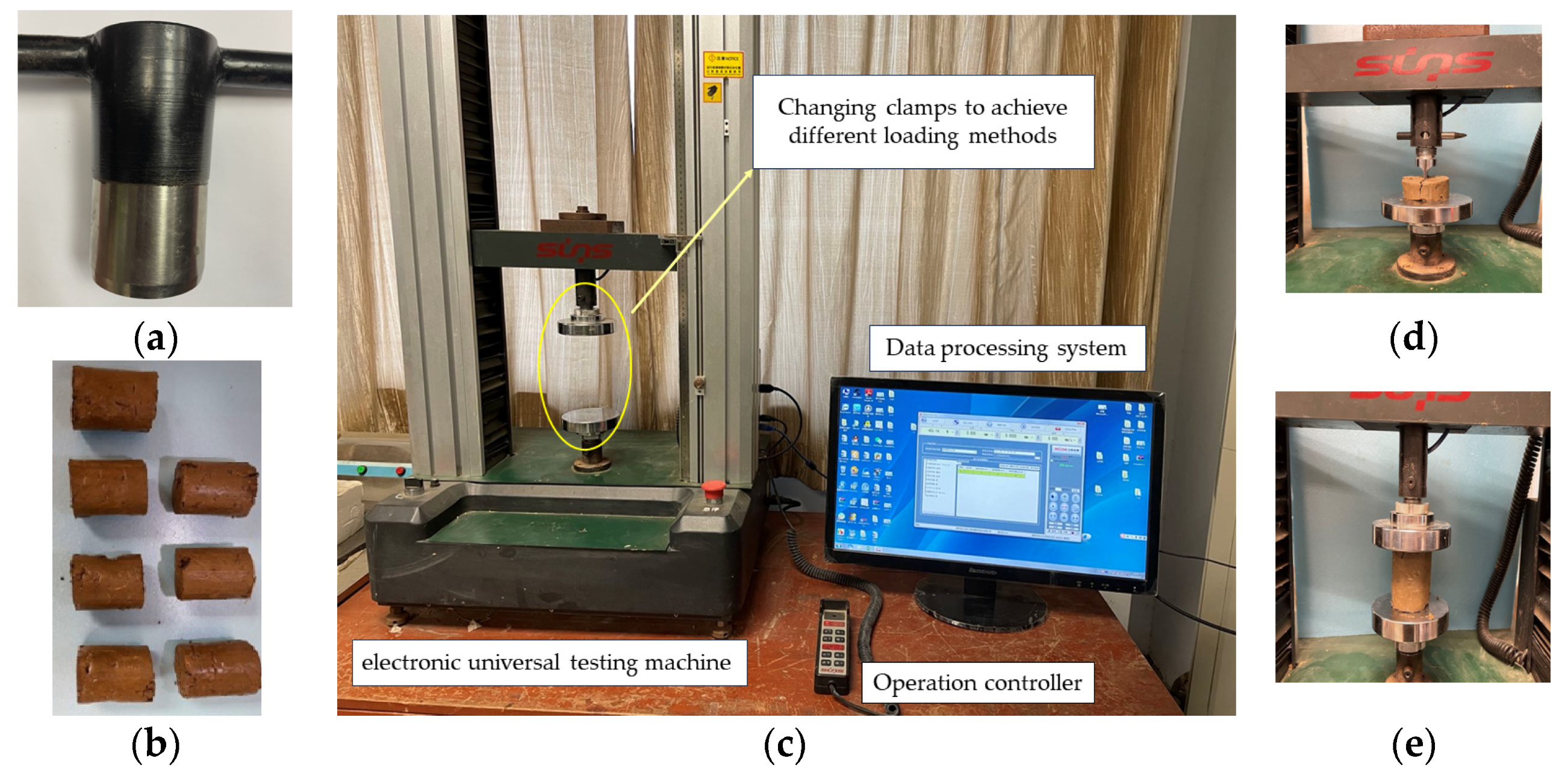The test response values are the maximum compressive strength (represented by the corresponding force) (F_C) obtained from the unconfined compressive strength test and the maximum shear force (F_S) obtained from the shear test. Paddy soil was sampled from the rice–wheat rotation trial site of the Chinese Academy of Agricultural Sciences. The agronomy of the sampling area was subjected to rice–wheat rotation, and the sampling period was the wheat–after–rice sowing period. The inside of the sampling tool was lubricated to minimize the friction between the tool and the soil. The sampling tool was inserted slowly and upright into the soil, and the soil was subsequently cut from the bottom of the container. Then, the handle was removed, and a cylindrical soil block with good regularity as the test sample was selected. The universal testing machine speed was set to 60 mm/min. The test was conducted at 0.5% strain reading to record the axial pressure until the sample deformation value reached 25 mm, and then the experiment was stopped. Before the shear test, a soil cutter was used to divide each test sample into 3 pieces transversely. Then, the shear sample is placed on the test bed so that the shearing knife is located in the symmetrical center of the sample. The shear test speed is set to 60 mm/min, and the shearing knife passes through the sample to stop the test. The maximum shear force during the shearing process is taken as the shear strength index. The physical tests are shown in Figure 2.

The bonding parameters of particles are mainly obtained through numerical simulation test calibration. The values of critical normal stress (C_N) and critical shear stress (C_S) are mainly concentrated in 2 × 10⁴ ~ 4 × 10⁵ Pa [24,25]. There are significant differences in the values of normal/shear stiffness per unit area (S_N/S_S) during different experimental processes, mainly using three orders of magnitude: 5 × 10⁶, 5 × 10⁷, and 1 × 10⁸ N/m³. The values of shear modulus (G) are mainly in the order of 1 × 10⁶, 1 × 10⁷, and 1 × 10⁸ Pa. However, the values of the simulation parameters are very much related to their models, so the selection of a suitable range of values for the above parameters is the basis for accurate simulation.

Parameter combinations of stiffness and shear modulus of the above orders of magnitude were used to conduct simulation tests (the critical stresses were taken as average values), and the effects of these factors on the compressive strength and deformation (Fc-x) curves were investigated. In the simulation experiment, the soil-related discrete element parameters are derived from experimental measurements and references (

Table 1. Discrete element parameter settings for EDEM simulation experiments.

Item	Steel	Soil
Density/(kg·m−3)	7850	2600
Shear modulus/Pa	7.9 × 1010	1.0 × 106
Poisson ratio	0.30	0.38
Rolling friction coefficient (Interaction with soil)	0.6	0.35
Static friction coefficient (Interaction with soil)	0.05	0.65
Restitution coefficient (Interaction with soil)	0.6	0.12
interfacial surface energy (Interaction with soil)/J/m2	---	3.90

) [27,32,33]. The remaining settings of the simulation test are the same as those of the actual test. The results of the simulation tests were compared with the actual physical test results to select the suitable parameter ranges. The test scheme and results are shown in

Table 2. Design and results of a preliminary determination of the parameter range by simulation.

Test Number	G (Pa)	SN/SS (N/m3)	CN/CS (Pa)	FC (N)
1	1 × 106	5 × 106	2.1 × 105	73.3
2	1 × 106	5 × 107	2.1 × 105	592.9
3	1 × 106	1 × 108	2.1 × 105	558
4	6 × 107	5 × 106	2.1 × 105	69.4
5	6 × 107	5 × 107	2.1 × 105	713.1
6	6 × 107	1 × 108	2.1 × 105	1369.3
7	1 × 108	5 × 106	2.1 × 105	70.2
8	1 × 108	5 × 107	2.1 × 105	703
9	1 × 108	1 × 108	2.1 × 105	1325

. On the basis of the obtained parameter ranges, a single-factor simulation test of the stiffness was conducted to further determine the value range of the stiffness.

2.3. P-BD Tests

During mechanized seeding, the implements primarily compress and shear the soil. Therefore, with F_C and F_S as the response values, the parameters with significant impact were screened using the PB test method. The test factors include two parts: one is the parameters that were uncalibrated in the study of DEM simulation of paddy soil after rotary tillage; the other is the bonding parameters. Preliminary experiments show that when the soil–soil rolling friction coefficient was 0.35, there was a better fitting result. So, the value range of the static friction coefficient was set to 0.40~0.80. The value range of S_N/S_S was 0.5 × 10⁷ ~ 1.3 × 10⁷ N/m³, and the value range of C_N/C_S was 0.2 × 10⁵ ~ 4 × 10⁵ Pa. The PB test scheme and results are shown in

Table 3. Design and results of P-BD tests.

Test Number	SF	SN (N/m3)	SS (N/m3)	CN (Pa)	CS (Pa)	FC (N)	FS (N)
1	0.40	1.3 × 107	0.5 × 107	4.0 × 105	4.0 × 105	90.1	7.35
2	0.40	1.3 × 107	1.3 × 107	4.0 × 105	0.2 × 105	107.7	5.85
3	0.40	0.5 × 107	0.5 × 107	4.0 × 105	0.2 × 105	64.6	4.98
4	0.40	0.5 × 107	0.5 × 107	0.2 × 105	0.2 × 105	63.6	4.78
5	0.40	0.5 × 107	1.3 × 107	0.2 × 105	4.0 × 105	135.4	8.76
6	0.40	1.3 × 107	1.3 × 107	0.2 × 105	4.0 × 105	165.3	8.93
7	0.80	0.5 × 107	0.5 × 107	0.2 × 105	4.0 × 105	82.2	4.99
8	0.80	1.3 × 107	1.3 × 107	0.2 × 105	0.2 × 105	121.4	6.89
9	0.80	0.5 × 107	1.3 × 107	4.0 × 105	0.2 × 105	101.9	5.09
10	0.80	0.5 × 107	1.3 × 107	4.0 × 105	4.0 × 105	167.1	9.92
11	0.80	1.3 × 107	0.5 × 107	0.2 × 105	0.2 × 105	117.8	7.25
12	0.60	0.9 × 107	0.9 × 107	2.1 × 105	2.1 × 105	133.6	8.39
13	0.80	1.3 × 107	0.5 × 107	4.0 × 105	4.0 × 105	118.9	7.9

.

2.4. Optimization Experiment of Significant Parameters

Response surface tests and parameter optimization fitting analysis were performed to obtain the optimal parameter combination scheme of the integrated model. The test factors were the significant influencing parameters selected from the P-BD test. Since the C_N is a factor with insignificant influence in this test model, the C_N value was taken as 2.1 × 10⁵ Pa for the test. Therefore, the C_S value range in the test was set to 0.2 × 10⁵ ~ 2 × 10⁵ Pa. The test response values are F_C and F_S. The test scheme and results are shown in

Table 4. Design and results of the Box–Behnken test for optimization experiment of significant parameters.

Test Number	SN (N/m3)	SS (N/m3)	CS (Pa)	FC (N)	FS (N)
1	0.9 × 107	1.3 × 107	0.2 × 105	106.7	5.66
2	0.9 × 107	0.5 × 107	2.0 × 105	92.5	6.19
3	0.9 × 107	1.3 × 107	2.0 × 105	179.7	10.2
4	1.3 × 107	0.9 × 107	0.2 × 105	123.6	7.3
5	1.3 × 107	1.3 × 107	1.1 × 105	192.5	11.42
6	0.9 × 107	0.5 × 107	0.2 × 105	92.1	6.05
7	0.5 × 107	1.3 × 107	1.1 × 105	151.5	9.39
8	1.3 × 107	0.9 × 107	2.0 × 105	154.2	9.39
9	0.5 × 107	0.9 × 107	0.2 × 105	102.2	5.38
10	1.3 × 107	0.5 × 107	1.1 × 105	106.1	7.24
11	0.5 × 107	0.5 × 107	1.1 × 105	74.3	4.82
12	0.9 × 107	0.9 × 107	1.1 × 105	133.9	8.39
13	0.5 × 107	0.9 × 107	2.0 × 105	112.3	7.04

. The optimization scheme of parameter combination was obtained using design-expert software. The obtained parameter optimization schemes were simulated, respectively, and the simulation experiments were compared with the actual experiments to determine the optimal parameter combination scheme.

2.5. Analysis of Relative Errors

The difference between the DEM simulation and the actual test is an important indicator for evaluating the accuracy of the model and related parameters. Therefore, the wheat planter, widely used in rice–wheat rotation systems, was selected for error analysis between simulations and field trials further to evaluate the accuracy of the discrete element parameters. In addition, the lateral relative error ($\delta$) of wheat seeds was used as the response value, as the agronomic goal of this sowing method was to sow wheat evenly and completely within the 240 mm seed strip.

The operating parameters of the implements, such as forward speed (V₀), seeding quantity (S_Q), and rotary tillage speed (N_T), influence the lateral relative error of wheat seeds during operation [34]. The parameter ranges of the implement were forward speed: 0.8~1.6 m/s, seeding quantity: 150~300 kg/hm², and rotary tillage speed: 180~280 rpm. The level of each factor was altered separately to investigate the influence of each factor on the relative error (the other two factors were considered the middle-value level), and the lateral error change was statistically analyzed. In the simulation experiment of the sowing process, the soil-related discrete element parameters are derived from Table 1 and experimental measurements. According to the actual measurement, the wheat discrete element model is 6.9 mm in length, 3.4 mm in width, and 3 mm in height, and the discrete element parameters of wheat grains came from references [35,36]. The wheat grain density is 1350 Kg/m³, Poisson’s ratio is 0.29, and shear modulus is 5.1 × 10⁸ Pa.

Table 5. Discrete element parameter settings for seeding simulation experiments.

Item	Steel	Wheat	Soil
Rolling friction coefficient (Interaction with wheat)	0.05	0.08	0.29
Static friction coefficient (Interaction with wheat)	0.4	0.58	0.48
Restitution coefficient (Interaction with wheat)	0.5	0.41	0.13
Interfacial surface energy (Interaction with wheat)/J/m2	---	---	1.69

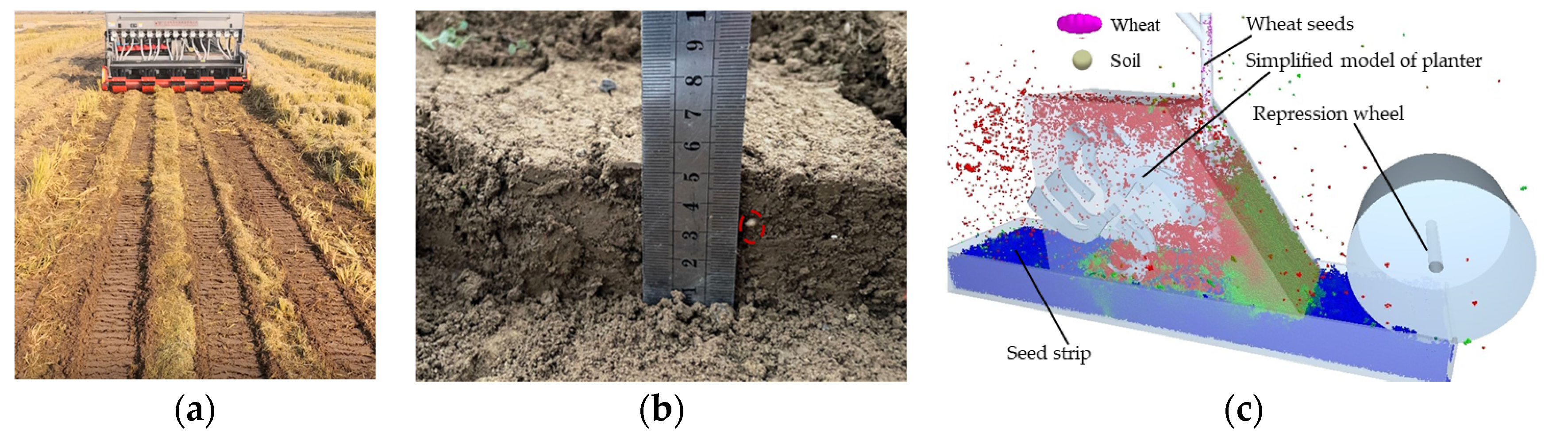
shows the relevant parameter settings for discrete element simulation. Figure 3 depicts a comparison test of the relative error analysis for the simulation and the actual operation.

The Box–Behnken design test was used to analyze further the relative error range and the interaction of each parameter with the relative error under the DEM model and the parameter values. The lateral distribution error of wheat seeds during the simulation and test was counted using V₀, S_Q, and N_T as influencing factors (

Table 6. Design and results of the Box–Behnken test for the analysis of error range.

Test Number	V0	SQ	NT	$\mathit{\delta }$
1	0.8	15	180	14.27
2	1.2	10	280	22.36
3	1.6	10	230	12.34
4	1.2	15	230	12.3
5	1.2	15	230	11.36
6	1.6	20	230	8.87
7	1.6	15	180	12.02
8	0.8	15	280	24.81
9	1.2	10	180	10.63
10	1.6	15	280	15.94
11	1.2	15	230	12.81
12	1.2	15	230	10.78
13	0.8	20	230	14.59
14	1.2	15	230	13.69
15	0.8	10	230	19.28
16	1.2	20	280	18.73
17	1.2	20	180	9.12

).

3. Results and Discussion

3.1. Result Analysis of Parameter Range Determination Experiment

The test results for the maximum compression force in the unconfined test are 105.43 N, 125.56 N, 154.27 N, 120.71 N, and 11.61 N, and the test results for the maximum shear force are 6.22 N, 7.63 N, 8.38 N, 6.92 N and 8.13 N. The physical test results show that the average maximum compression force of unconfined compression is 123.52 N, and the average maximum shear force is 7.46 N. 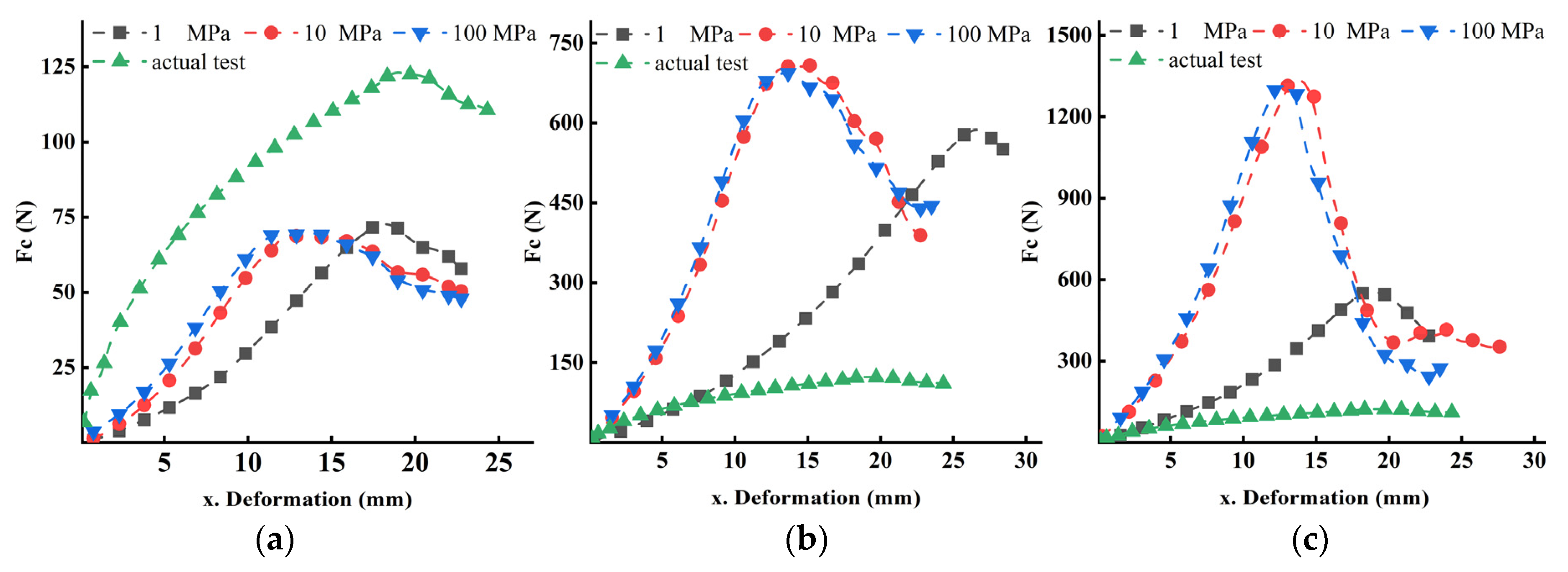To further analyze the influence of parameter combination schemes on the unconfined compression test process, the F_C-x diagram of each group of tests in Table 1 was extracted, drawn, and compared with the F_C-x curve variation law of the actual test, as shown in Figure 4. As can be seen from Table 1, the F_C is in the order of 0.7 × 10², 5 × 10², and 1 × 10³ N when the stiffness is 5 × 10⁶, 5 × 10⁷, and 1 × 10⁸ N/m³, respectively. At stiffnesses of 5 × 10⁷ or 1 × 10⁸ N/m³, the simulation test values have large differences from the actual test values. When the stiffness is 5 × 10⁶ N/m³, the simulation test results are 73.3, 69.4, and 70.4 N, which are closest to the actual test values. From Figure 4, it can be seen that with an increase in shear modulus, the deformations corresponding to the maximum values of the simulation tests are shifted forward. When the shear modulus value is 1 Mpa, the deformation corresponding to the maximum value of the simulation experiment is the closest to the deformation amount corresponding to the maximum value of the actual test. The values of shear modulus and stiffness were initially determined to be 1 MPa and 5 × 10⁶ N/m³.

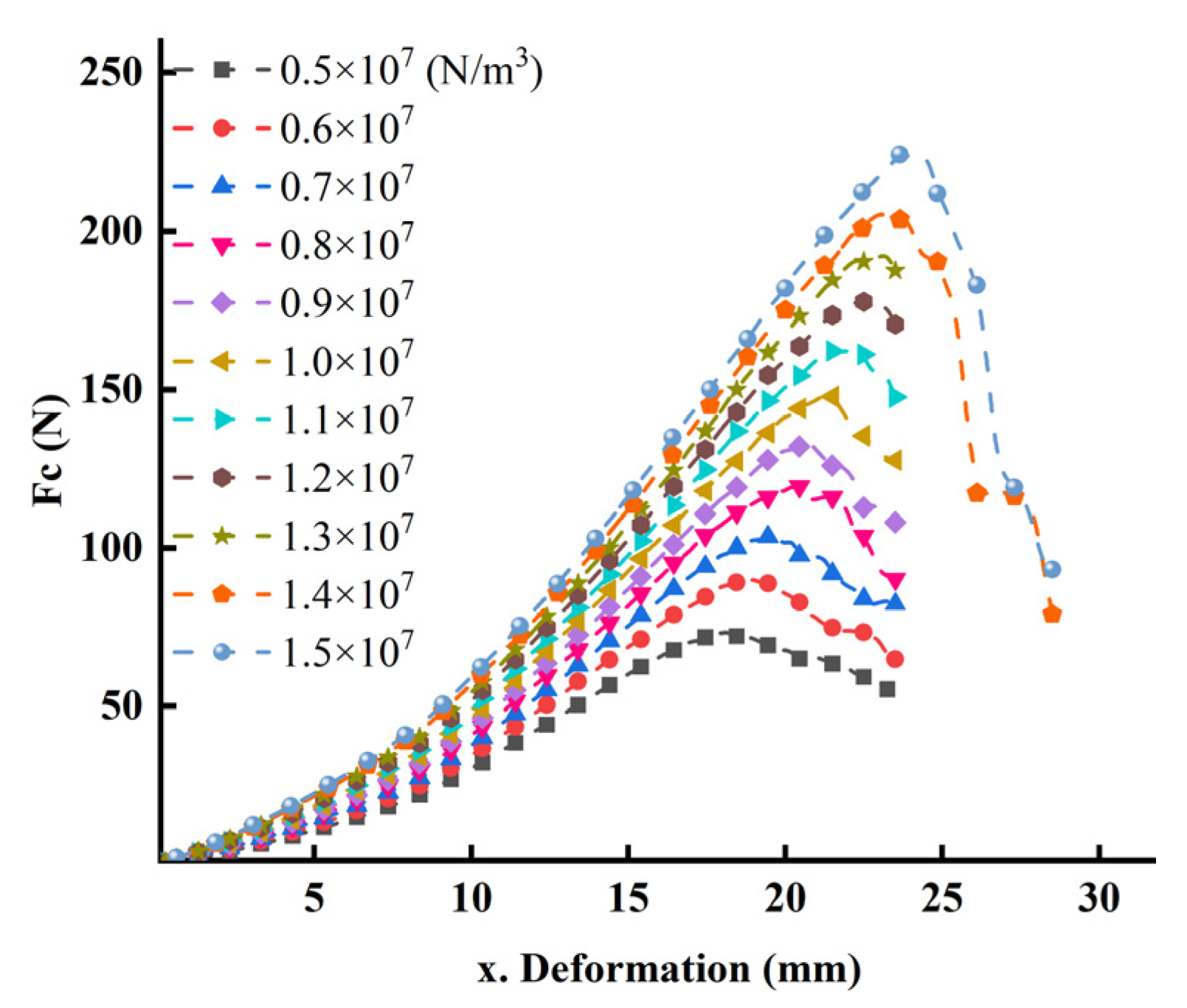
As shown in Figure 5, the simulation test results of unconfined compressive strength with a shear modulus of 1mpa, a critical stress of 2.1 × 10⁵ Pa, and a stiffness range of 0.5 × 10⁷ ~ 1.5 × 10⁷ N/m³. As seen from Figure 5, with an increase in stiffness per unit area, the value of F_C shows an increasing trend, and the deformation corresponding to the maximum value of Fc also increases in response. When the stiffness per unit area is greater than 1.3 × 10⁷ N/m³, the value of F_C is greater than 200 N, and the curve is quite different from the actual test curve. Therefore, the value range of the stiffness per unit area for subsequent tests was determined to be 0.5 × 10⁷ ~ 1.3 × 10⁷ N/m³.

3.2. P-BD Test Analysis

Table 7. Significant analysis results of parameters by P-BD test.

Terms	Source of Contribution	Stdized Effect	Sum of Squares	Contribution/%	Order of Significance
FC	SF	13.77	568.56	3.32	4
	SN	17.73	943.41	5.52	3
	SS	43.6	5702.88	33.34	1
	CN	−5.9	104.43	0.61	5
	CS	30.33	2760.33	16.14	2
FS	SF	0.23	0.16	0.35	4
	SN	0.94	2.66	5.75	3
	SS	1.37	5.59	12.09	2
	CN	−0.09	0.02	0.05	5
	CS	2.17	14.11	30.51	1

shows the influence of each test factor on the unconfined compressive strength and shear force. Both experimental indicators (F_C and F_S) increase with an increase in S_F, S_N, S_S, and C_S, while they decrease with an increase in C_N. The contribution of both factors, S_F and C_N, to both test metrics is less than 5%. Based on the integration model, the order of significance on F_C is S_S, C_S, S_N, S_F, and C_N, and the order of significance on Fs is C_S, S_S, S_N, S_F, and C_N. S_N, S_S, and C_S are factors that have a significant effect on all indexes.

3.3. Result Analysis of Parameter Optimization Test

The design-expert software was used to analyze these experimental data, and the ANOVA after merging the insignificant terms is shown in

Table 8. Variance analysis of the Box–Behnken test for parameters optimization.

Terms	Source	Sum of Squares	df	Mean Square	F-Value	p-Value
FC	Model	14,065.09	4	3516.27	23.43	0.0002	***
	SN	2315.40	1	2315.40	15.43	0.0044	***
	SS	8804.64	1	8804.64	58.66	<0.0001	***
	CS	1627.35	1	1627.35	10.84	0.0110	**
	SSCS	1317.69	1	1317.69	8.78	0.0181	**
	Residual	1200.80	8	150.10
	Cor Total	15,265.89	12
FS	Model	42.36	4	10.59	11.50	0.0021	***
	SN	9.50	1	9.50	10.32	0.0124	**
	SS	19.13	1	19.13	20.77	0.0019	***
	CS	8.88	1	8.88	9.65	0.0145	**
	SSCS	4.84	1	4.84	5.26	0.0510	**
	Residual	7.37	8	0.9207
	Cor Total	49.72	12

Note: ***, extremely significant (p < 0.01); **, significant (0.01 < p < 0.05).

. From the results of the ANOVA on F_C, it can be seen that the p-value in the regression model is 0.0002 (p < 0.01), indicating that the regression model is extremely significant. Regression terms S_N and S_S are extremely significant for F_C, and regression terms C_S and S_SC_S are significant for F_C. From the results of the ANOVA on F_S, it can be seen that the p-value in the regression model is 0.0021 (p < 0.01), indicating that the regression model is highly significant. The effect of the regression term S_S on F_S is highly significant, and the effect of regression terms S_N, C_S, and S_SC_S on the F_S model is significant. From the analysis of the F-value of each factor, it can be seen that the order of significance of the effect of each factor on both the F_C model and F_S model is S_S > S_N > C_S. Regression models of F_C and F_S with each significant term were developed, respectively, as shown in Equations (1) and (2).

$${\mathrm{F}}_{\mathrm{C}}=44.30+42.531\times S_N+27.48\times S_S-29.53\times C_S+50.42\times S_S{C}_S$$

(1)

$${\mathrm{F}}_{\mathrm{S}}=3.38+2.73\times S_N+0.50\times S_S-1.60\times C_S+3.06\times S_S{C}_S$$

(2)

From Table 8, it can be seen that the S_SC_S term has a significant effect on F_C and a relatively significant effect on F_S. The effect patterns of the S_SC_S interaction on F_C and F_S were further analyzed separately. When the value of S_N is taken at the center position (0.9 × 10⁷ N/m³), the interaction of S_S and C_S on F_C and F_S is shown in Figure 6. Both F_C and F_S show an increasing trend with an increase in S_S or C_S. The overall influence trend for each factor on F_C and F_S is that F_C and F_S increase with an increase in S_N, S_S, and C_S, respectively, among which the S_S factor causes the largest increase in F_C and F_S, and the C_S factor causes F_C and F_S showed the smallest increase.

To accurately simulate the compression and shear properties of soil at the same time, a multi-objective variable optimization method was adopted to solve the model optimization with F_C value and F_S in the actual test as the objectives. The optimized parameter combination schemes are obtained. That is, S_N is 1.07 × 10⁷ N/m³, S_S is 0.70 × 10⁷ N/m³, and C_S is 0.35 × 10⁵ Pa, corresponding F_C and F_S are 120.1 N and 7.70 N, respectively.

3.4. Effect Analysis of Factors on Relative Error

3.4.1. Effect of Forward Speed on Relative Error

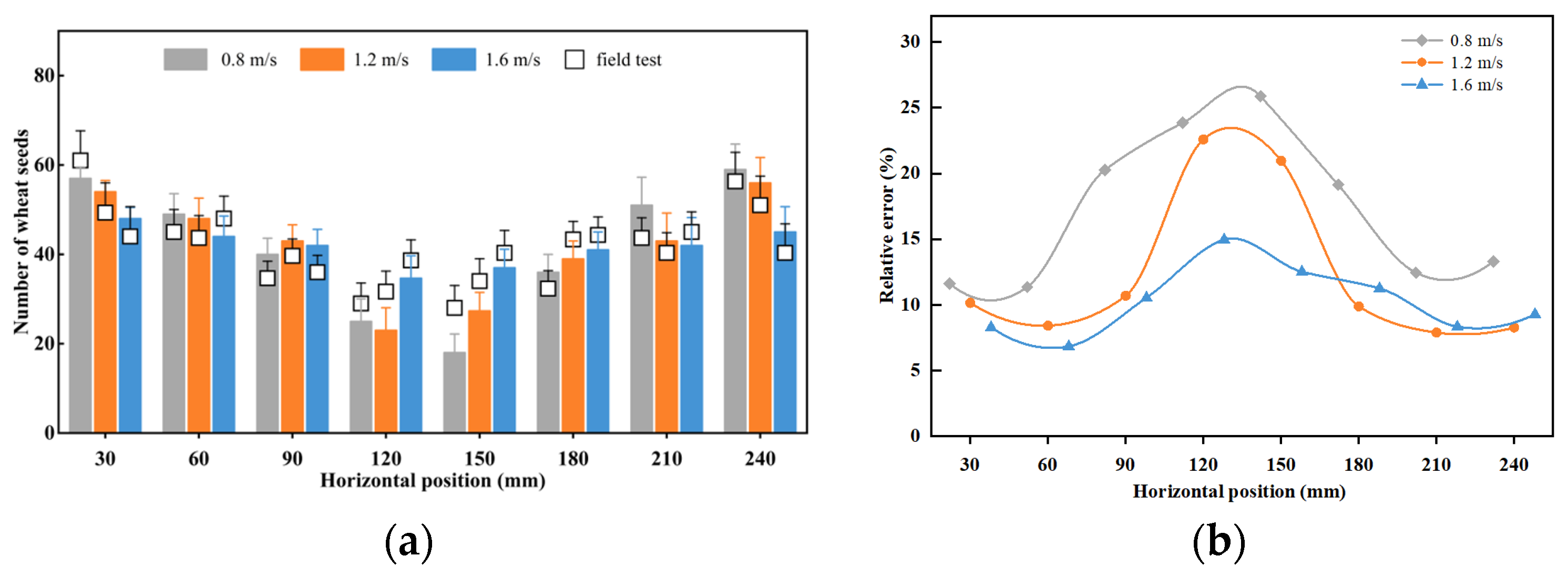
DEM simulations and actual tests were conducted for seeding operation processes with forward speeds of 0.8, 1.2, and 1.6 m/s. The distribution of wheat seeds in the soil was then determined and compared under the three working conditions. The wheat seeds in the simulation and test exhibit similar distribution rules when the simulation and test analyses are combined (Figure 7). Seed distribution generally exhibited a pattern of less distribution in the middle of the seed belt and more distribution on both sides of the seed belt. The distribution of seeds tended to increase gradually from the middle to the sides. In addition, as forward speed increased, this trend gradually weakened, i.e., the difference in the number of wheat seeds between the middle and sides of the strip gradually decreased.

The relative error under each working condition exhibited a trend of smaller relative error on the sides of the seed belt and a significant relative error in the middle of the seed belt. When the forward speed of the implement was 0.8, 1.2, and 1.6 m/s, the minimum relative errors were 11.24%, 7.87%, and 6.83%; the maximum relative errors were 25.87%, 22.58%, and 14.96%; and the average relative errors were 17.37%, 12.35%, and 10.24%, respectively. It can be seen that the relative errors between the simulation and actual test show a decreasing trend with an increase in the forward speed when the average relative errors under different working conditions are compared.

3.4.2. Effect of Seeding Quantity on Relative Error

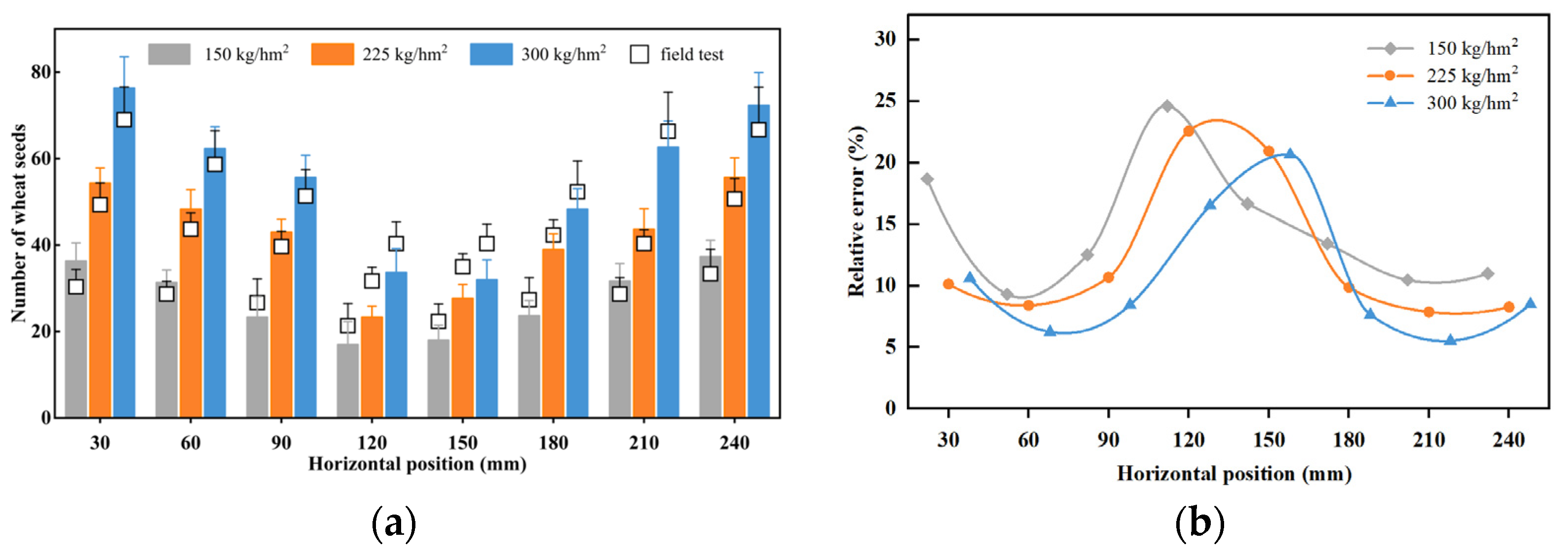
The DEM simulation and actual experiment were compared and analyzed under seeding quantities of 150, 225, and 300 kg/hm². The distribution of wheat seeds in the soil and relative errors were counted under the three working conditions (Figure 8). The results of the simulation and field test showed the same change law; that is, wheat seeds in the soil were distributed less in the middle of the seed belt but more distributed in the edges of the seed belt. When the seeding quantity was 150, 225, and 300 kg/hm², the minimum relative errors were 9.30%, 7.87%, and 6.25%; the maximum relative errors were 24.62%, 22.58%, and 20.66%; and the average relative errors were 14.58%, 12.35%, and 10.52%, respectively.

3.4.3. Effect of Rotary Tillage Speed on Relative Error

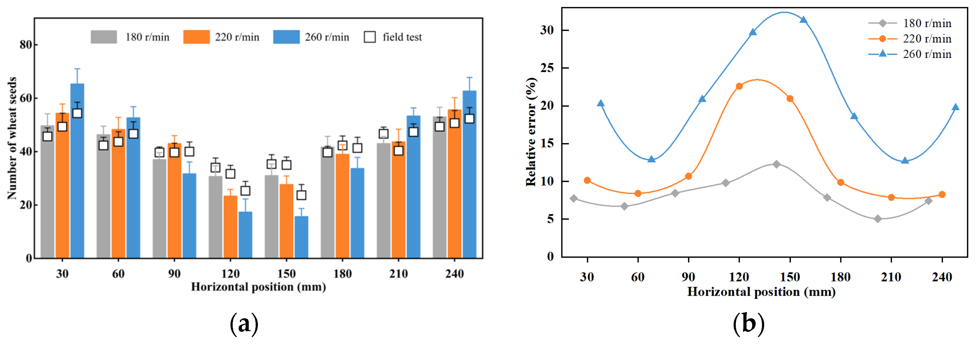
The DEM simulation and the actual test were compared and analyzed at three different rotary tillage speeds: 180, 230, and 280 rpm. The distribution of wheat seeds in the soil and relative errors were counted under the three working conditions (Figure 9). These seeds in the soil were distributed less in the middle of the seed belt but more distributed at the edges of the seed belt. However, the occurrence of seeds gathering at the edges became more obvious as the rotary tillage speed increased. Simultaneously, the presence of seeds gathering at the edges was more obvious in the simulation than in the actual operation. When the rotary tillage speeds were 180, 230, and 260 r/min, the minimum relative errors per cell were 5.04%, 7.87%, and 12.67%; the maximum relative errors per cell were 12.26%, 22.58%, and 31.30%; and the average relative errors were 8.42%, 12.35%, and 21.29%, respectively. The relative errors per cell in the middle of the seed strip were significant, while the relative errors per cell at the edges of the seed strip were small. Further, the relative error varied greatly at different rotary tillage speeds, with the smallest relative error at 180 r/min and the greatest relative error at 280 rpm.

3.5. Analysis of Error Range

Table 9. Variance analysis of regression equation of the Box–Behnken test for the analysis of error range.

Source	Sum of Squares	df	Mean Square	F-Value	p-Value
Model	316.35	9	35.15	19.40	0.0004	***
V0	70.69	1	70.69	39.02	0.0004	***
SQ	22.11	1	22.11	12.21	0.0101	**
NT	160.20	1	160.20	88.44	<0.0001	***
V0SQ	0.3721	1	0.3721	0.2054	0.6641
V0NT	10.96	1	10.96	6.05	0.0435	**
SQNT	1.12	1	1.12	0.6203	0.4568
V02	10.32	1	10.32	5.70	0.0484	**
SQ2	0.0010	1	0.0010	0.0006	0.9815
NT2	38.04	1	38.04	21.00	0.0025	***
Lack of fit	7.35	3	2.45	1.84	0.2801
Cor Total	329.03	16

Note: ***, extremely significant (p < 0.01); **, significant (0.01 < p < 0.05).

presents the results of the ANOVA and shows that the p-value of the regression model is p = 0.0004 < 0.01, and that of the lack of fit is p = 0.2801 > 0.1. This indicates that the regression model is extremely significant and the lack of fit is insignificant, implying that the model is well-fitted and highly reliable. Furthermore, p-value analysis of each factor reveals that the terms V₀, N_T, and N_T² (square term of N_T) have a highly significant effect on the model. In contrast, S_Q, V₀N_T (interaction term of V₀ and N_T), and V₀² (square term of V₀) have a significant effect on the model. In addition, the order of significance of the effect of each factor on relative error was N_T > V₀ > S_Q. Therefore, a quadratic regression model of the relative error and three key factors (V₀, S_Q, N_T) was established, as shown in Equation (3).

$$\begin{array}{c}\delta =55.935-14.172V_0-0.046S_Q-0.333N_T+0.153V_0{S}_Q\\ -0.083V_0{N}_T+0.002S_Q{N}_T+9.79V_0{}^2+0.001S_Q{}^2+0.001N_T{}^2\end{array}$$

(3)

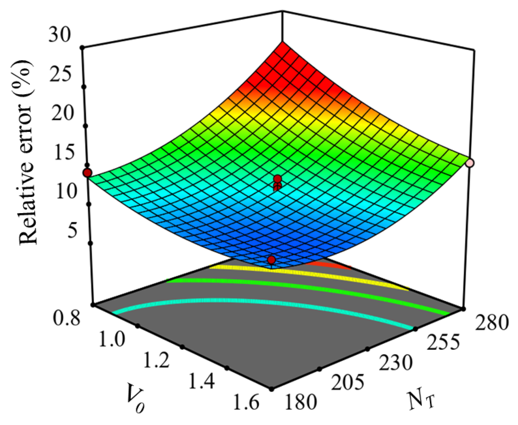
The interaction effect model of V₀ and N_T on the relative error when the S_Q was at the middle level (225 kg/hm²) is shown in Figure 10. The relative error showed a gradually decreasing trend with an increase in V₀; with an increase in N_T, the relative error initially decreased and then increased.

The regression equation was solved, and the relative error range was found to range from 8.8% to 28.4% when the value range of the factors was combined. The minimum relative error between the simulation and the actual experiment is 8.8% when the parameter combination is V₀ = 1.4 m/s, S_Q = 300 kg/hm², and N_T = 205 rpm. The simulation has the maximum relative error with the actual experiment, which is 28.4% when the parameter combinations are V₀ = 0.8 m/s, S_Q = 150 kg/hm², and N_T = 280 rpm.

4. Discussions

Compared with related studies, the accuracy of the results of this study can be compared and analyzed. Ding [25] research results show that the stiffness per unit area and critical stress of paddy soil are of the order of magnitude of 10⁷ N/m³ and 10⁵ Pa, respectively, and the lower the soil layer, the larger the parameter. This is consistent with the results of this study. Fang’s [26,27] research results show that the rotary tillage operation can be simulated accurately when the shear modulus is set to 1 MPa. Li et al. investigated the crushing characteristics of agglomerate soil blocks using the shear test. The results show that the values of normal stiffness per unit area, shear stiffness per unit area, critical normal stress, and critical shear stress are 2.86 × 10⁶ N·m⁻², 1.64 × 10⁶ N·m⁻², 2.42 × 10⁵ Pa, and 1.47 × 10⁵ Pa, respectively [24]. The results of the corresponding parameters in this study are S_N of 1.07 × 10⁷ N/m³, S_S of 0.70 × 10⁷ N/m³, and C_S of 0.35 × 10⁵ Pa, respectively. The two are in the same order of magnitude, and the difference is not huge. The main sources of difference are the differences in soil quality and moisture content. The results of these studies are the same in order of magnitude, and the difference is not significant. The main sources of difference are the differences in soil quality and moisture content. This shows the accuracy of this study.

Under different rotary tillage speeds, the possible reasons for the errors between simulation and actual values are as follows. This may be due to the soil composition and surface structure being more complex in the actual operation process, making wheat seeds enter the soil crevices more quickly and thus remain in their original position.

The relative average error between the simulation and actual test showed a gradual decreasing trend with increasing seeding quantity; however, this trend was not particularly obvious. Nevertheless, it can be seen that the differences in the relative error values per cell are small under different seeding quantities, comparing the relative error per cell of the simulation and test under different seeding quantities. It showed a regular pattern of a significant relative error per cell in the middle region of the seed strip and a smaller relative error per cell at the edges of the seed strip. This may be because as the seeding quantity increases, the probability of seed–seed interaction increases, and the probability of seed–soil interaction decreases with an increase in seeding quantity, resulting in a decrease in the cumulative relative error.

The reasons for the interaction effect of V₀ and N_T on the relative error are as follows. This may be because with an increase in V₀ or a decrease in N_T, the interval for soil cutting increases. The smaller the effective action area between wheat seed and soil, the shorter the effective action time. Hence, the value of accumulated relative error is smaller. However, as N_T increases, so does the speed of the rotary cutter tip and the ability of the rotary cutter to throw particles to the seed strip edges, resulting in a large amount of wheat seed in the middle of the seed belt being thrown to the edges, thus increasing the relative error increases.

5. Conclusions

This study conducted a simulation of paddy soil with high moisture content and high viscosity based on the Hertz–Mindlin JKR + Bonding Integrated Model. The influence of each planter operation parameter on the relative error is evaluated by comparing the DEM simulation and the actual test results. It facilitates visual study of the kinematic properties during seed–soil interaction during sowing and suppression.

(1) When the shear modulus value is 1 Mpa, the deformation corresponding to the maximum value of the simulation experiment is the closest to the deformation amount corresponding to the maximum value of the actual test; the difference between the simulation curve and the actual test curve is small when the ranges of the stiffness per unit area form 0.5 × 10⁷ ~ 1.3 × 10⁷ N/m³.

(2) The overall influence trend of each factor on F_C and F_S is that F_C and Fs increase with an increase in S_N, S_S, and C_S, respectively, among which S_S factor causes the largest increase in F_C and F_S, and C_S factor causes F_C and F_S showed the smallest increase. There is a minimum relative error (6.05%) when S_N is 1.07 × 10⁷ N/m³, S_S is 0.70 × 10⁷ N/m³, and C_S is 0.35 × 10⁵ Pa, corresponding to F_C and F_S of 120.1 N and 7.70 N, respectively.

(3) The sequence of effects of each factor on the relative error was N_T > V₀ > S_Q. The average relative errors were 17.04%, 12.35%, and 9.02% when V₀ was 0.8, 1.2, and 1.6 m/s, respectively. The average relative errors were 14.58%, 12.35%, and 10.52% when S_Q was 150, 225, and 300 kg/hm², respectively. The average relative errors were 8.42%, 12.35%, and 21.29% when N_T was 180 rpm, 230 rpm, and 280 rpm, respectively. In addition, combined with the value range of these factors, the range of relative error was found to be from 8.8% to 28.4%.

References

- Yuan, G.; Huan, W.; Song, H.; Lu, D.; Chen, X.; Wang, H.; Zhou, J. Effects of Straw Incorporation and Potassium Fertilizer on Crop Yields, Soil Organic Carbon, and Active Carbon in the Rice–Wheat System. Soil Tillage Res. 2021, 209, 104958. [Google Scholar] [CrossRef]
- Singh, A.; Phogat, V.K.; Dahiya, R.; Batra, S.D. Impact of Long-Term Zero till Wheat on Soil Physical Properties and Wheat Productivity under Rice–Wheat Cropping System. Soil Tillage Res. 2014, 140, 98–105. [Google Scholar] [CrossRef]
- Ahmad, F.; Weimin, D.; Qishou, D.; Rehim, A.; Jabran, K. Comparative Performance of Various Disc-Type Furrow Openers in No-Till Paddy Field Conditions. Sustainability 2017, 9, 1143. [Google Scholar] [CrossRef]
- Li, C.; Tang, Y.; McHugh, A.D.; Wu, X.; Liu, M.; Li, M.; Xiong, T.; Ling, D.; Tang, Q.; Liao, M.; et al. Development and Performance Evaluation of a Wet-Resistant Strip-till Seeder for Sowing Wheat Following Rice. Biosyst. Eng. 2022, 220, 146–158. [Google Scholar] [CrossRef]
- Fengwei, G.; Youqun, Z.; Feng, W.; Zhichao, H.; Lili, S. Simulation Analysis and Experimental Validation of Conveying Device in Uniform Rrushed Straw Throwing and Seed-Sowing Machines Using CFD-DEM Coupled Approach. Comput. Electron. Agric. 2022, 193, 106720. [Google Scholar] [CrossRef]
- Tang, H.; Xu, C.; Xu, W.; Xu, Y.; Xiang, Y.; Wang, J. Method of Straw Ditch-Buried Returning, Development of Supporting Machine and Analysis of Influencing Factors. Front. Plant Sci. 2022, 13, 967838. [Google Scholar] [CrossRef] [PubMed]
- Xi, X.; Gu, C.; Shi, Y.; Zhao, Y.; Zhang, Y.; Zhang, Q.; Jin, Y.; Zhang, R. Design and Experiment of No-Tube Seeder for Wheat Sowing. Soil Tillage Res. 2020, 204, 104724. [Google Scholar] [CrossRef]
- Kaur, M.; Singh, D.; Anand, A.; Singh, T. Do Attributes of Happy Seeder Technology Influence Its Adoption Speed? An Investigation Using Duration Analysis in Northern India. Int. J. Agric. Sustain. 2023, 21, 2198324. [Google Scholar] [CrossRef]
- Tang, H.; Xu, C.; Wang, Z.; Wang, Q.; Wang, J. Optimized Design, Monitoring System Development and Experiment for a Long-Belt Finger-Clip Precision Corn Seed Metering Device. Front. Plant Sci. 2022, 13, 814747. [Google Scholar] [CrossRef]
- Tang, H.; Xu, F.; Xu, C.; Zhao, J.; Wang, Y.-J. The Influence of a Seed Drop Tube of the Inside-Filling Air-Blowing Precision Seed-Metering Device on Seeding Quality. Comput. Electron. Agric. 2023, 204, 107555. [Google Scholar] [CrossRef]
- Coetzee, C.J. Review: Calibration of the Discrete Element Method. Powder Technol. 2017, 310, 104–142. [Google Scholar] [CrossRef]
- Horabik, J.; Molenda, M. Parameters and Contact Models for DEM Simulations of Agricultural Granular Materials: A Review. Biosyst. Eng. 2016, 147, 206–225. [Google Scholar] [CrossRef]
- Yinyan, S.; Man, C.; Xiaochan, W.; Odhiambo, M.O.; Weimin, D. Numerical Simulation of Spreading Performance and Distribution Pattern of Centrifugal Variable-Rate Fertilizer Applicator Based on DEM Software. Comput. Electron. Agric. 2018, 144, 249–259. [Google Scholar] [CrossRef]
- Tang, H.; Xu, C.; Zhao, J.; Wang, J. Stripping Mechanism and Loss Characteristics of a Stripping-Prior-to-Cutting Header for Rice Harvesting Based on CFD-DEM Simulations and Bench Experiments. Biosyst. Eng. 2023, 229, 116–136. [Google Scholar] [CrossRef]
- Ucgul, M.; Fielke, J.M.; Saunders, C. Three-Dimensional Discrete Element Modelling (DEM) of Tillage: Accounting for Soil Cohesion and Adhesion. Biosyst. Eng. 2015, 129, 298–306. [Google Scholar] [CrossRef]
- Ucgul, M.; Fielke, J.M.; Saunders, C. 3D DEM Tillage Simulation: Validation of a Hysteretic Spring (Plastic) Contact Model for a Sweep Tool Operating in a Cohesionless Soil. Soil Tillage Res. 2014, 144, 220–227. [Google Scholar] [CrossRef]
- Ucgul, M. Simulating Soil–Disc Plough Interaction Using Discrete Element Method–Multi-Body Dynamic Coupling. Agriculture 2023, 13, 305. [Google Scholar] [CrossRef]
- Ucgul, M.; Saunders, C. Simulation of Tillage Forces and Furrow Profile during Soil-Mouldboard Plough Interaction Using Discrete Element Modelling. Biosyst. Eng. 2020, 190, 58–70. [Google Scholar] [CrossRef]
- Bahrami, M.; Naderi-Boldaji, M.; Ghanbarian, D.; Ucgul, M.; Keller, T. Simulation of Plate Sinkage in Soil Using Discrete Element Modelling: Calibration of Model Parameters and Experimental Validation. Soil Tillage Res. 2020, 203, 104700. [Google Scholar] [CrossRef]
- Zhang, R.; Han, D.; Ji, Q.; He, Y.; Li, J. Calibration methods of sandy soil parameters in simulation of discrete element method. Trans. Chin. Soc. Agric. Mach. 2017, 48, 49–56. [Google Scholar] [CrossRef]
- Sun, J.; Liu, Q.; Yang, F.; Liu, Z.; Wang, Z. Calibration of discrete element simulation parameters of sloping soil on loess plateau and its interaction with rotary tillage components. Trans. Chin. Soc. Agric. Mach. 2022, 53, 63–73. [Google Scholar] [CrossRef]
- Hoseinian, S.H.; Hemmat, A.; Esehaghbeygi, A.; Shahgoli, G.; Baghbanan, A. Development of a Dual Sideway-Share Subsurface Tillage Implement: Part 1. Modeling Tool Interaction with Soil Using DEM. Soil Tillage Res. 2022, 215, 105201. [Google Scholar] [CrossRef]
- Zeng, Z.; MA, X.; Cao, X.; Li, Z.; Wang, X. Critical review of applications of discrete element method in agricultural engineering. Trans. Chin. Soc. Agric. Mach. 2021, 52, 1–20. [Google Scholar] [CrossRef]
- Li, Y.; Fan, J.; Hu, Z.; Luo, W.; Yang, H.; Shi, L.; Wu, F. Calibration of Discrete Element Model Parameters of Soil around Tubers during Potato Harvesting Period. Agriculture 2022, 12, 1475. [Google Scholar] [CrossRef]
- Ding, Q.; Ren, J.; Belal, E.A.; Zhao, J.; Ge, S.; Li, Y. DEM analysis of subsoiling process in wet clayey paddy soil. Trans. Chin. Soc. Agric. Mach. 2017, 48, 38–48. [Google Scholar] [CrossRef]
- Fang, H.; Ji, C.; Zhang, Q.; Guo, J. Force analysis of rotary blade based on distinct element method. Trans. Chin. Soc. Agric. Eng. 2016, 32, 54–59. [Google Scholar] [CrossRef]
- Fang, H.; Ji, C.; Ahmed, A.T.; Zhang, Q.; Guo, J. Simulation analysis of straw movement in straw-soil-rotary blade system. Trans. Chin. Soc. Agric. Mach. 2016, 47, 60–67. [Google Scholar] [CrossRef]
- Chen, G.; Wang, Q.; Li, H.; He, J.; Lu, C.; Zhang, X. Design and experiment of solid organic fertilizer crushing and striping machines. Trans. Chin. Soc. Agric. Eng. 2023, 39, 13–24. [Google Scholar]
- Aikins, K.A.; Ucgul, M.; Barr, J.B.; Awuah, E.; Antille, D.L.; Jensen, T.A.; Desbiolles, J.M.A. Review of Discrete Element Method Simulations of Soil Tillage and Furrow Opening. Agriculture 2023, 13, 541. [Google Scholar] [CrossRef]
- Tang, H.; Xu, W.; Zhao, J.; Xu, C.; Wang, J. Comparison of Rice Straw Compression Characteristics in Vibration Mode Based on Discrete Element Method. Biosyst. Eng. 2023, 230, 191–204. [Google Scholar] [CrossRef]
- Xie, F.; Wu, Z.; Wang, X.; Liu, D.; Wu, B.; Zhang, Z. Calibration of discrete element parameters of soils based on unconfined compressive strength test. Trans. Chin. Soc. Agric. Eng. 2020, 36, 39–47. [Google Scholar] [CrossRef]
- Ucgul, M.; Saunders, C.; Li, P.; Lee, S.-H.; Desbiolles, J.M.A. Analyzing the Mixing Performance of a Rotary Spader Using Digital Image Processing and Discrete Element Modelling (DEM). Comput. Electron. Agric. 2018, 151, 1–10. [Google Scholar] [CrossRef]
- Zhu, Q.; Wu, G.; Chen, L.; Zhao, C.; Meng, Z.; Shi, J. Structural design and optimization of seed separated plate of wheat wide-boundary sowing device. Trans. Chin. Soc. Agric. Eng. 2019, 35, 1–11. [Google Scholar]
- Luo, W.; Wu, F.; Gu, F.; Xu, H.; Wang, G.; Wang, B.; Yang, H.; Hu, Z. Optimization and Experiment of Fertilizer-Spreading Device for Wheat Wide-Boundary Sowing Planter under Full Rice Straw Retention. Agronomy 2022, 12, 2251. [Google Scholar] [CrossRef]
- Lu, C.; Gao, Z.; Li, H.; He, J.; Wang, Q.; Wei, X.; Wang, X.; Jiang, S.; Xu, J.; He, D.; et al. An Ellipsoid Modelling Method for Discrete Element Simulation of Wheat Seeds. Biosyst. Eng. 2023, 226, 1–15. [Google Scholar] [CrossRef]
- Liu, F.; Zhang, J.; Li, B.; Chen, J. Calibration of parameters of wheat required in discrete element method simulation based on repose angle of particle heap. Trans. Chin. Soc. Agric. Eng. 2016, 32, 247–253. [Google Scholar]
Figure 1.
The circulation planting process in the rice–wheat rotation system: (a) seedbed preparation before rice transplanting; (b) transplanting rice; (c) rice seedling growth; (d) rice field management; (e) rice harvest; (f) straw left in the field after rice harvest; (g) seedbed preparation before wheat sowing; (h) sowing wheat; (i) wheat germination; (j) wheat field management; (k) wheat harvest; (l) straw left in the field after wheat harvest.
Figure 2.
Physical tests to measure soil mechanical properties: (a) soil sample preparation tool; (b) physical test sample; (c) precision micro-control electronic universal testing machine; (d) shear strength test; (e) unconfined compressive strength test.
Figure 3.
Comparative tests of relative error analysis for simulation and actual operation: (a) actual operation of wheat–after–rice sowing in the field; (b) data measurement of wheat distribution under the soil; (c) simulation of wheat sowing process.
Figure 4.
Comparison of Fc-x curves between DEM simulation and physical experiments under different parameter conditions: (a) stiffness is 5 × 10⁶ N/m3; (b) stiffness is 5 × 10⁷ N/m3; (c) stiffness is 5 × 10⁸ N/m3.
Figure 5.
FC-x curves under different stiffness values.
Figure 6.
Effect of interaction between SS and CS on FC and FS: (a) the interaction effect between SS and CS on FC; (b) the interaction effect between SS and CS on FS.
Figure 7.
Comparison of differences between simulation and actual operation at different forward speeds: (a) Seeds distribution at different forward speeds; (b) Seeds relative error for simulation and actual operation at different forward speeds.
Figure 8.
Comparison of differences between simulation and actual operation at different seeding quantities: (a) Seeds distribution at different seeding quantities; (b) Seeds relative error for simulation and actual operation at different seeding quantities.
Figure 9.
Comparison of differences between simulation and actual operation at different rotary tillage speeds: (a) Seeds distribution at different rotary tillage speeds; (b) Seeds relative error for simulation and actual operation at different rotary tillage speeds.
Figure 10.
Effect of interaction between V0 and NT on relative error.