
Vibration Performance Analysis and Multi-Objective Optimization Design of a Tractor Scissor Seat Suspension System
Abstract
:1. Introduction
2. Methods
2.1. Main Effect Analysis
2.2. Analysis of Contribution
2.3. Gray Relation Analysis
2.4. Entropy Method
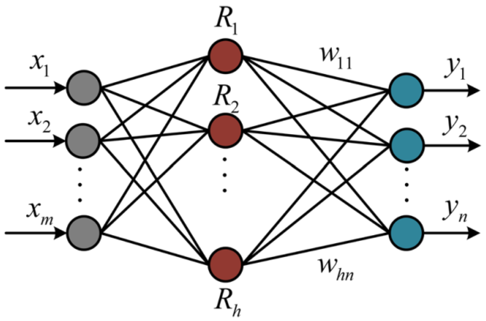
2.5. RBF Approximation Model
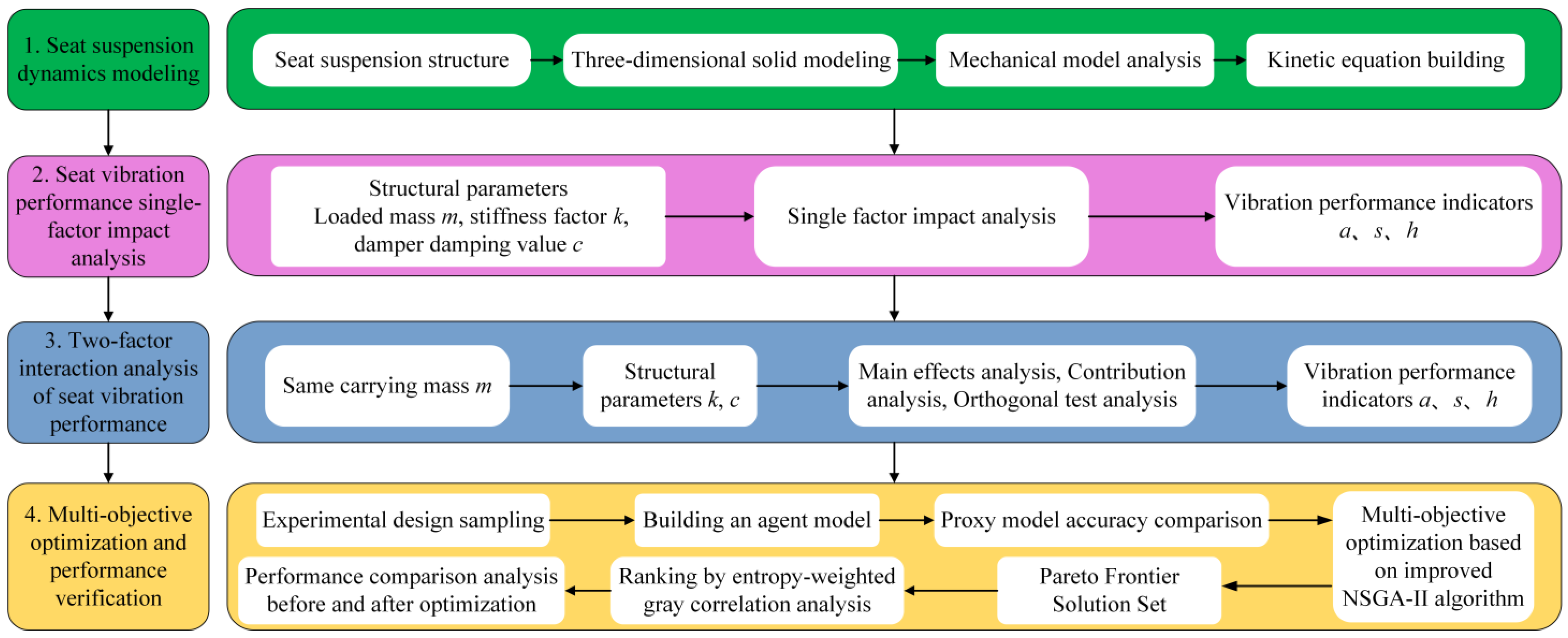
2.6. Optimize the Design Process
3. Scissor Seat Suspension Dynamics Model
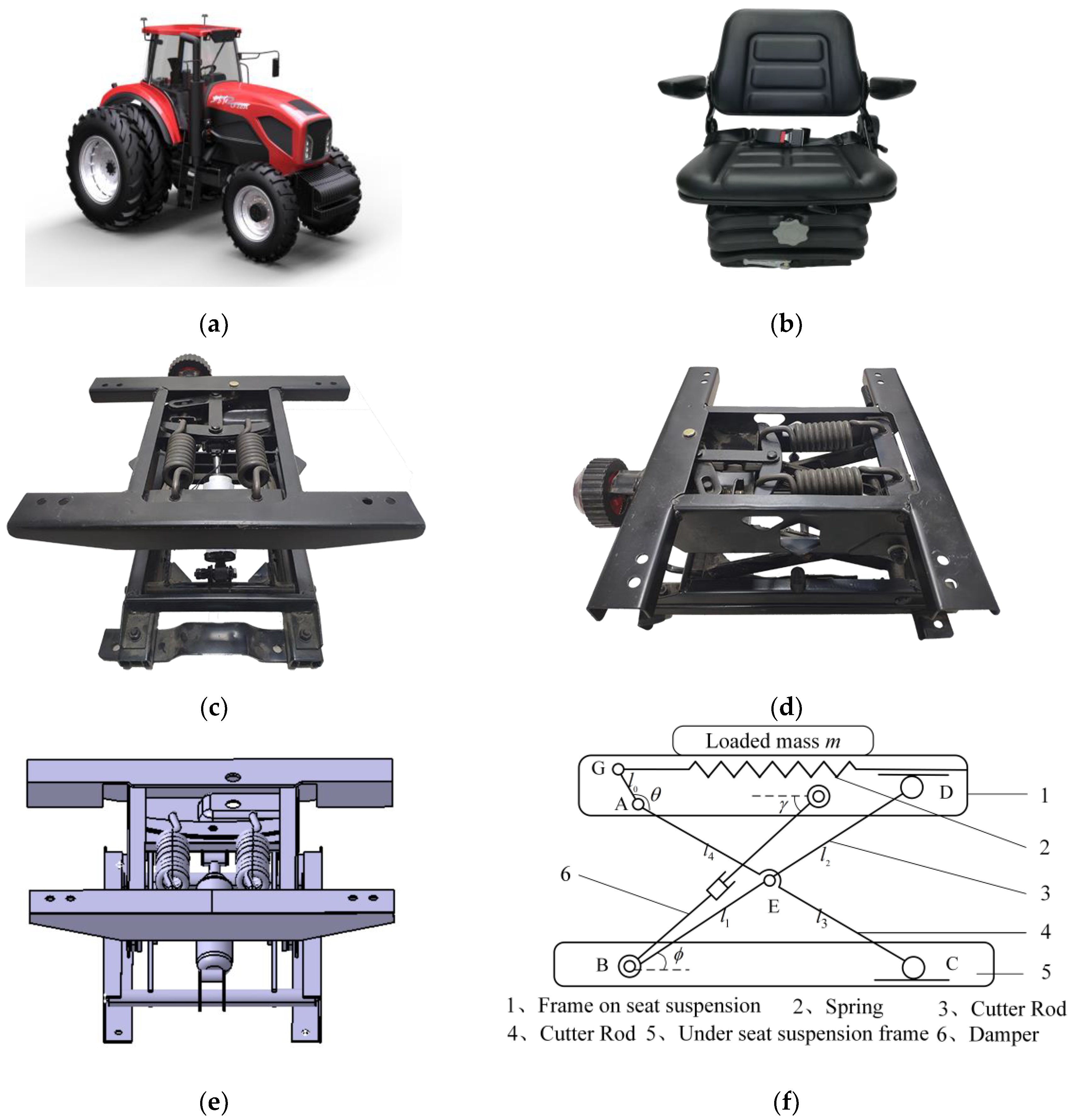
3.1. Seat Suspension Structure Form
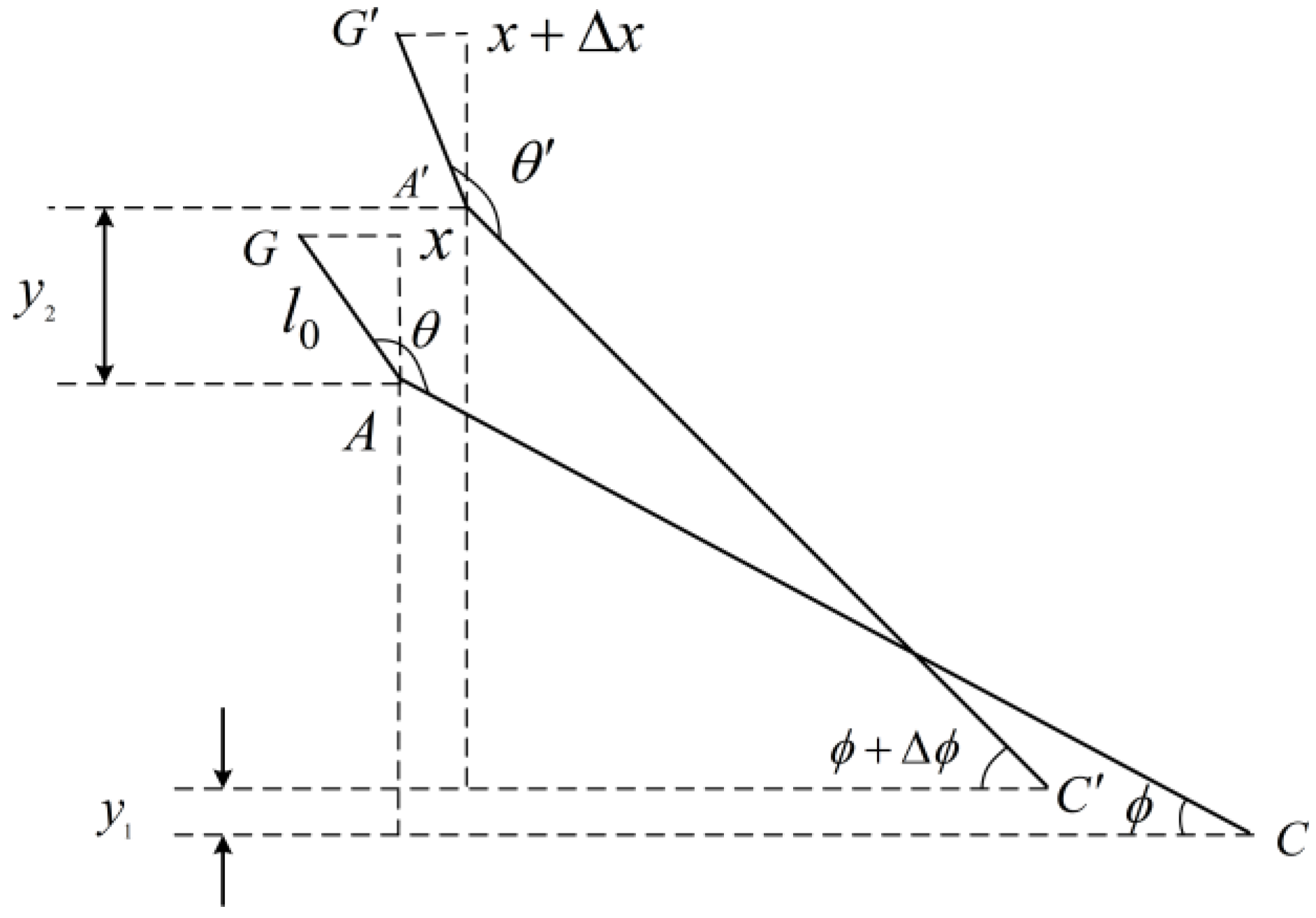
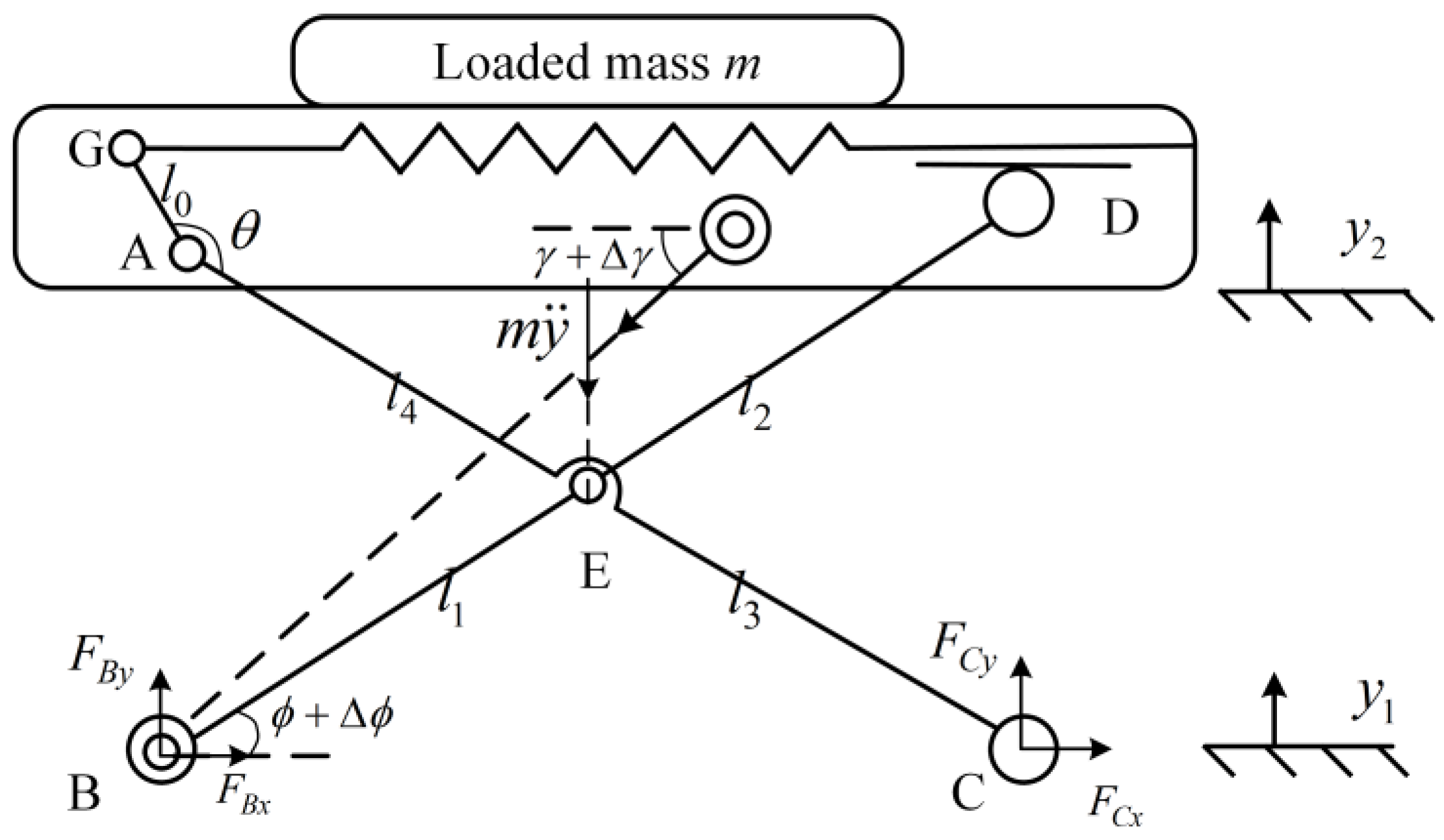
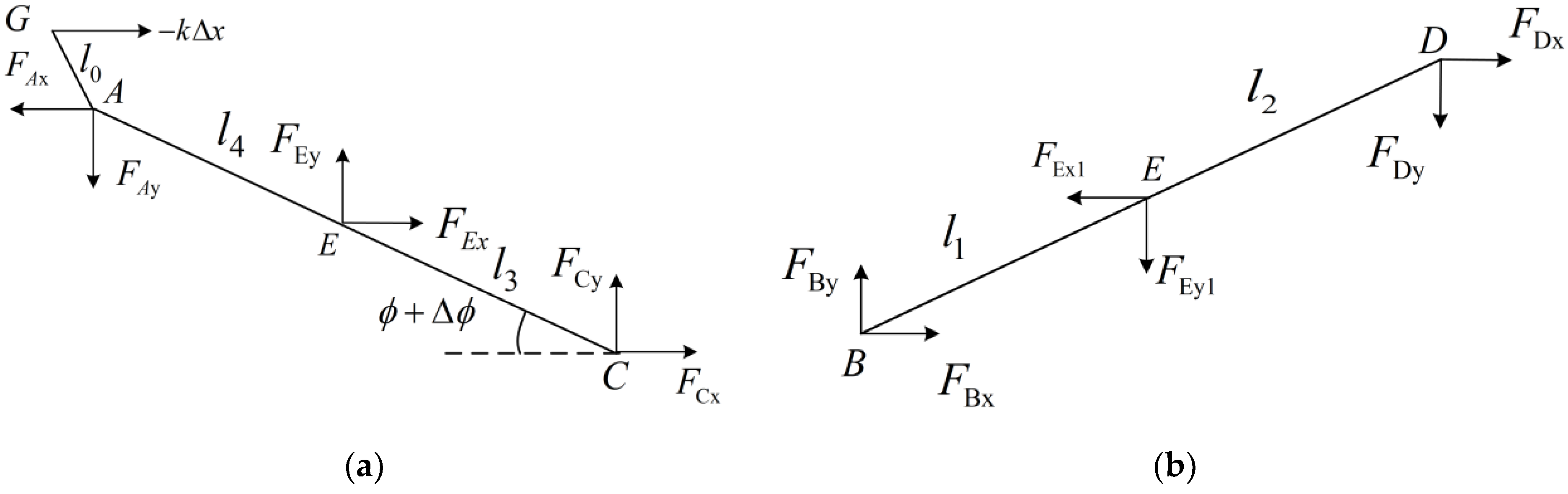
3.2. Seat Suspension Mechanics Model
4. Seat Suspension Vibration Performance Impact Analysis
4.1. Main Performance Parameters of the Seat Suspension
4.1.1. Stiffness Coefficient k
4.1.2. Damping Ratio ζ
4.1.3. Displacement s
4.1.4. Acceleration a
4.1.5. Transmission Rate η
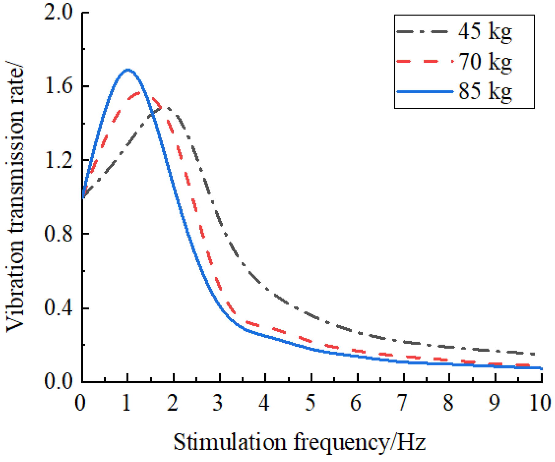
4.2. Load Quality Impact Analysis
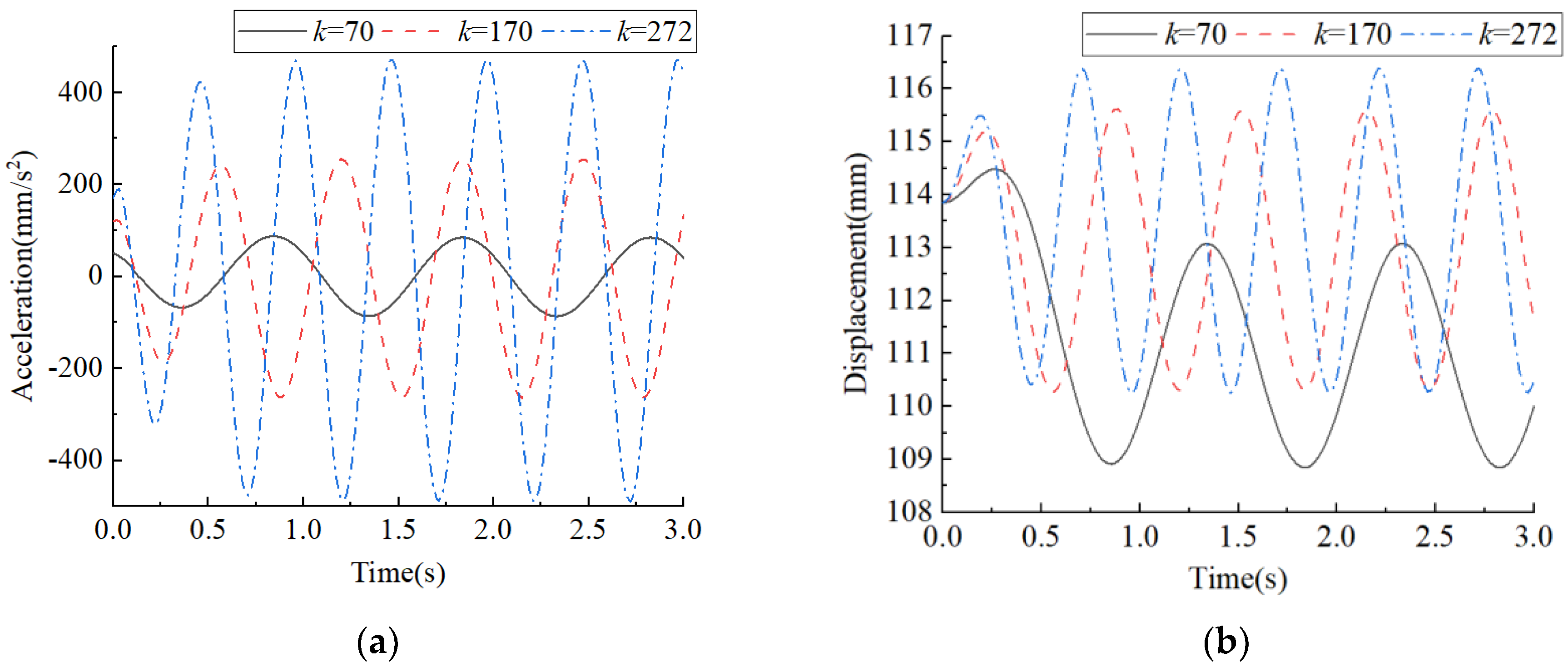
4.3. Spring Stiffness Coefficient Influence Analysis
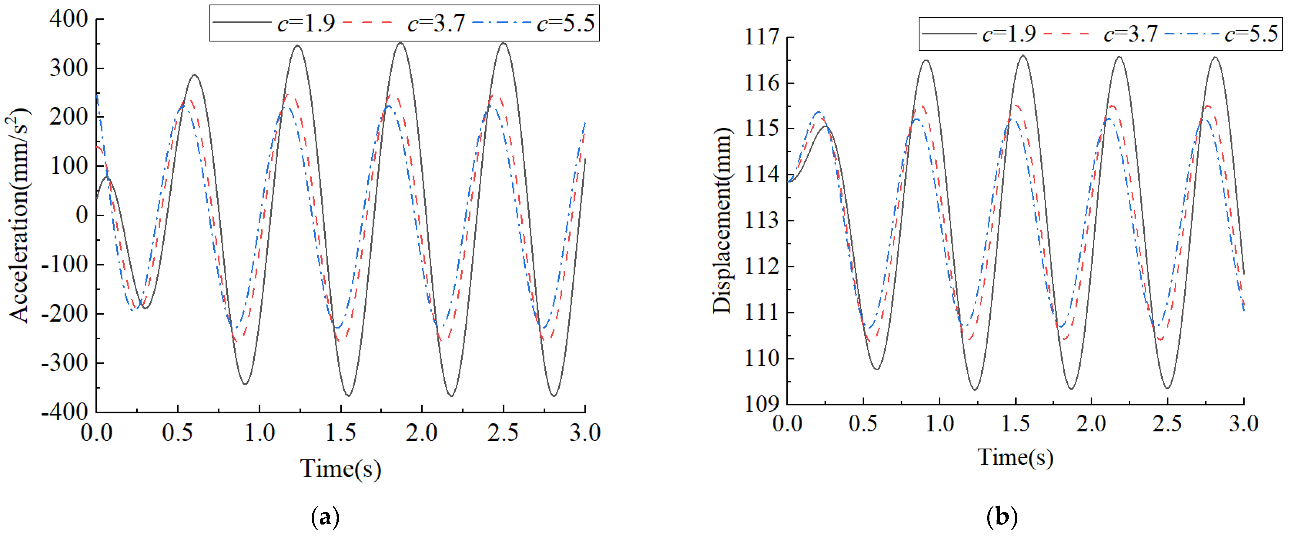
4.4. Damper Damping Influence Analysis
4.5. Analysis of Factors Influencing Different Performance Indicators
- (1)
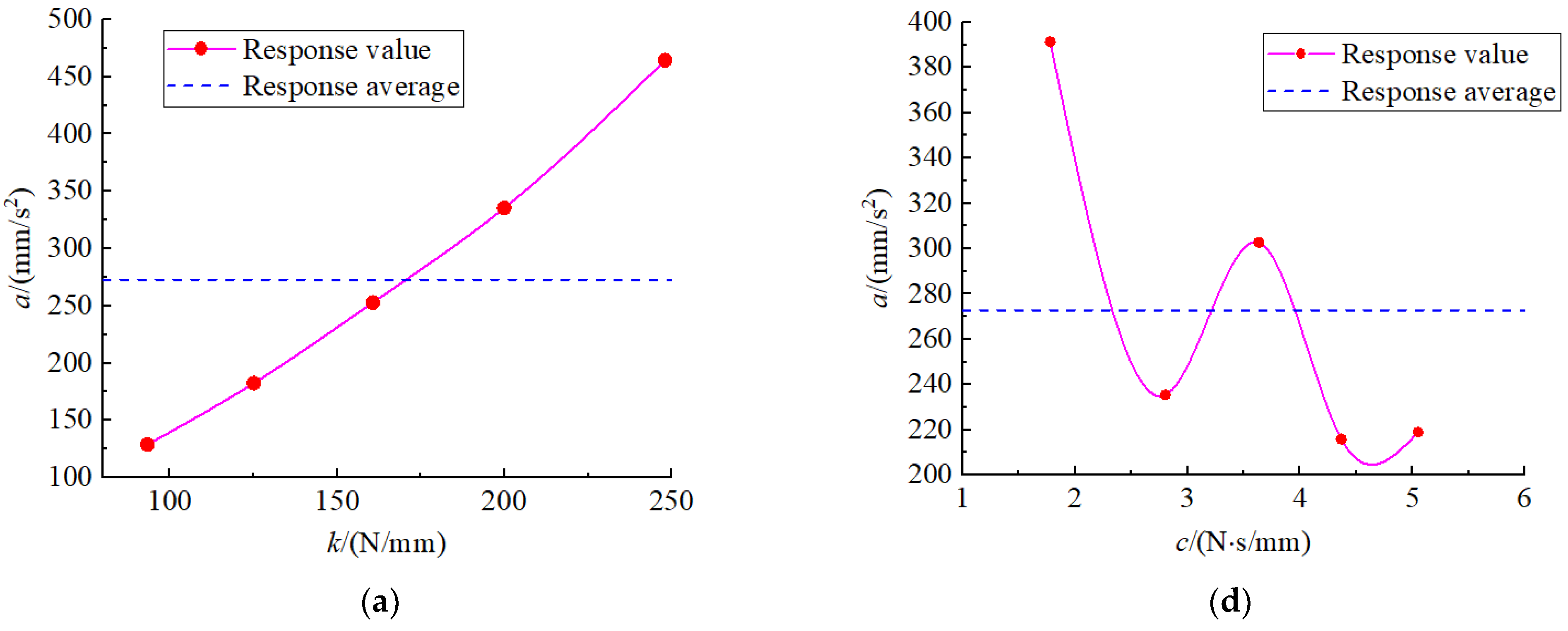
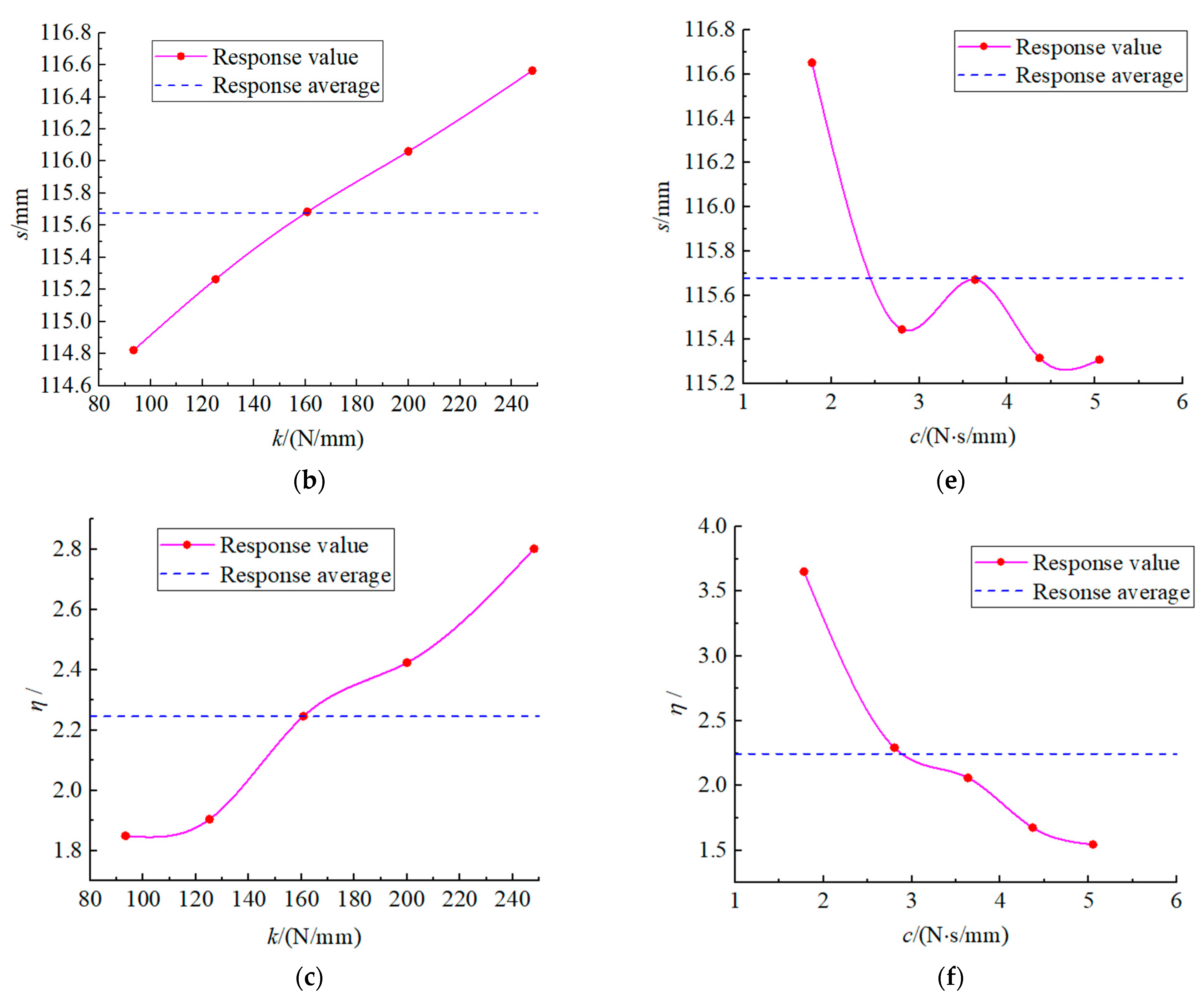
- Main Effect Analysis
- (2)
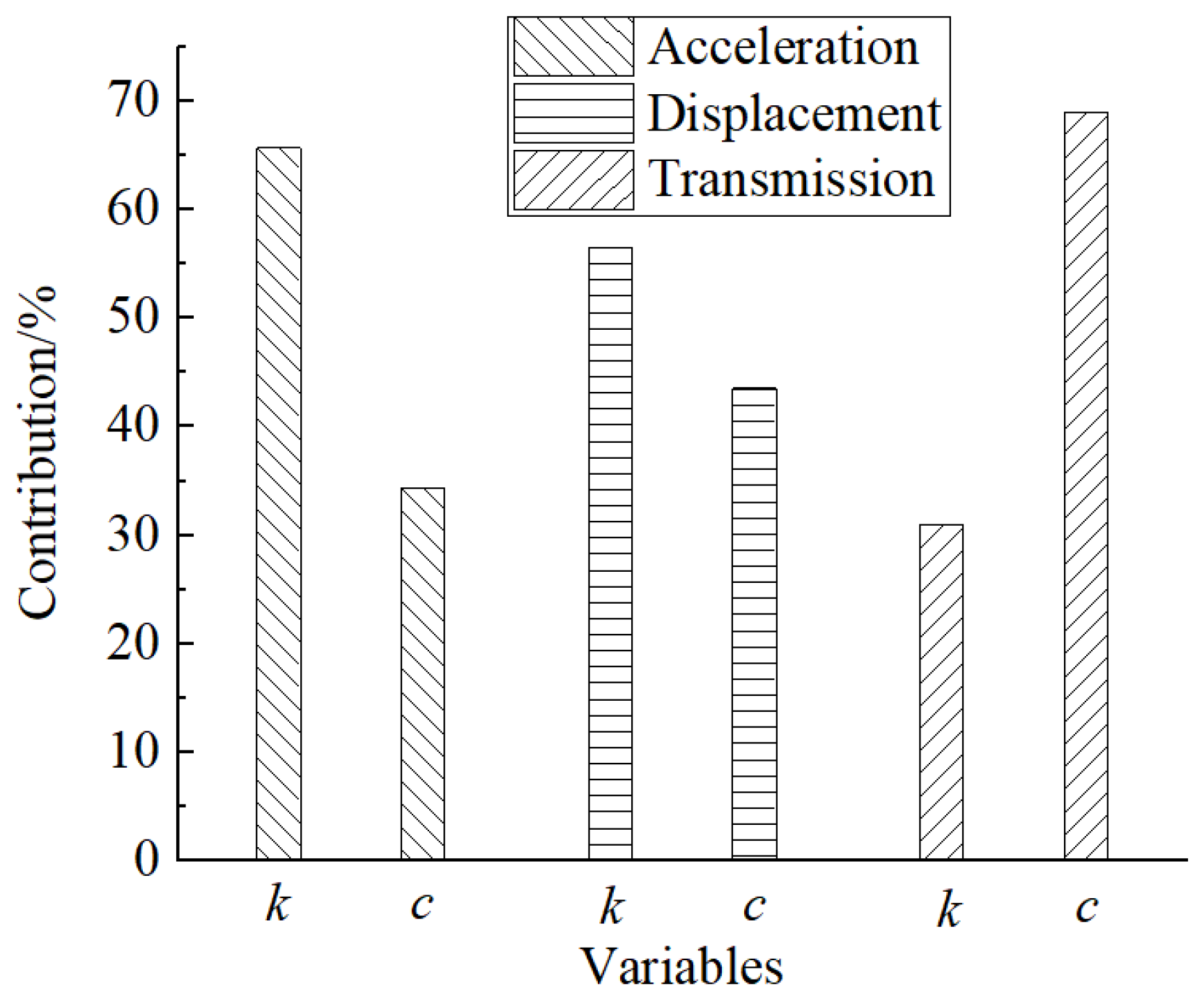
- Contribution analysis
5. Seat Suspension Vibration Attenuation Multi-Objective Optimization
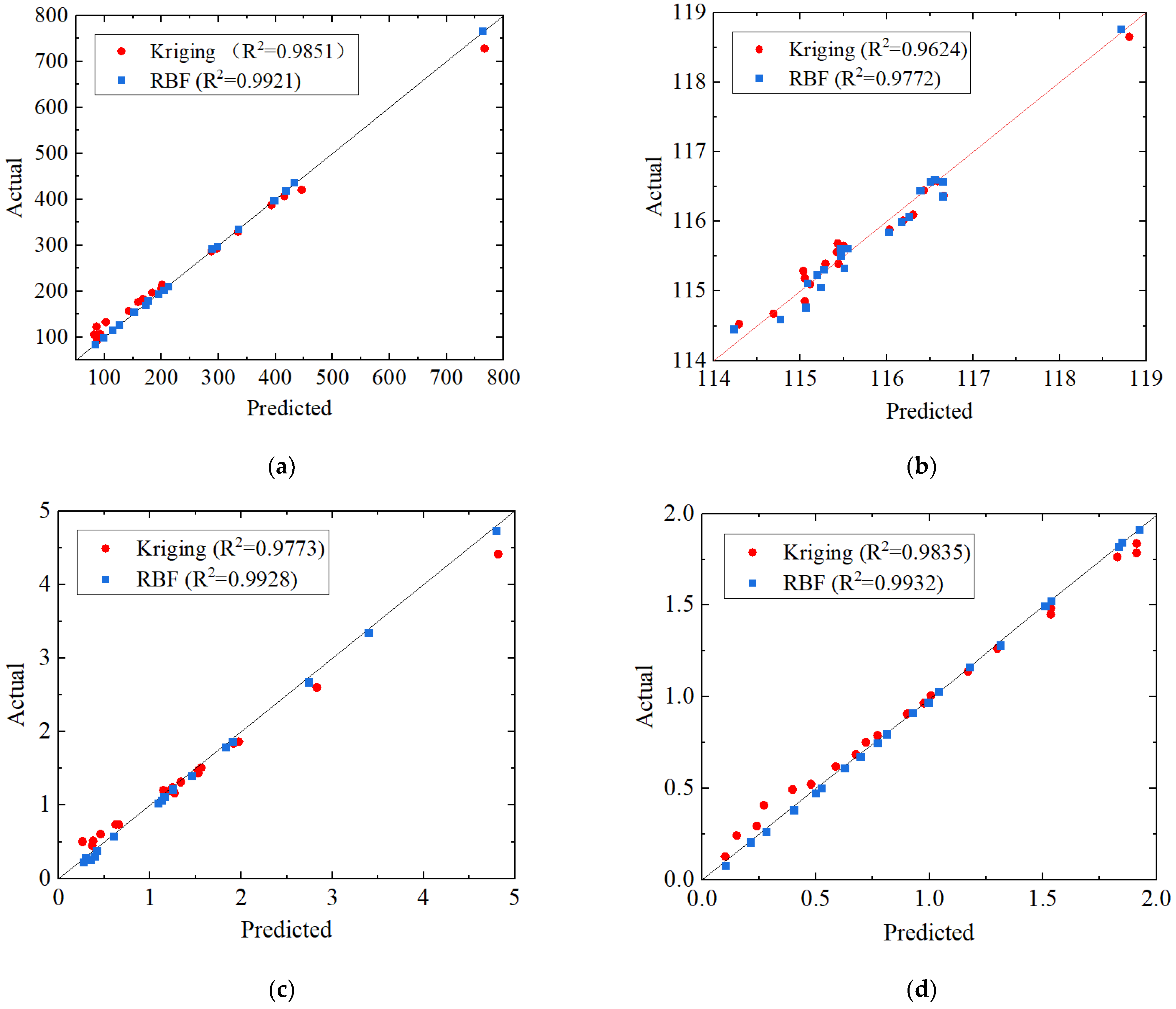
5.1. Approximate Model Approach
5.2. Multi-Objective Optimization Methods
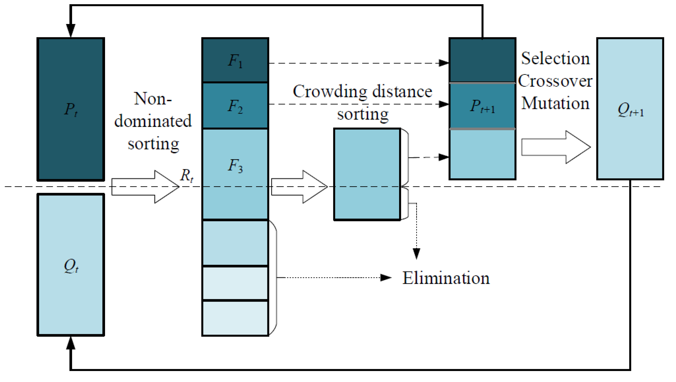
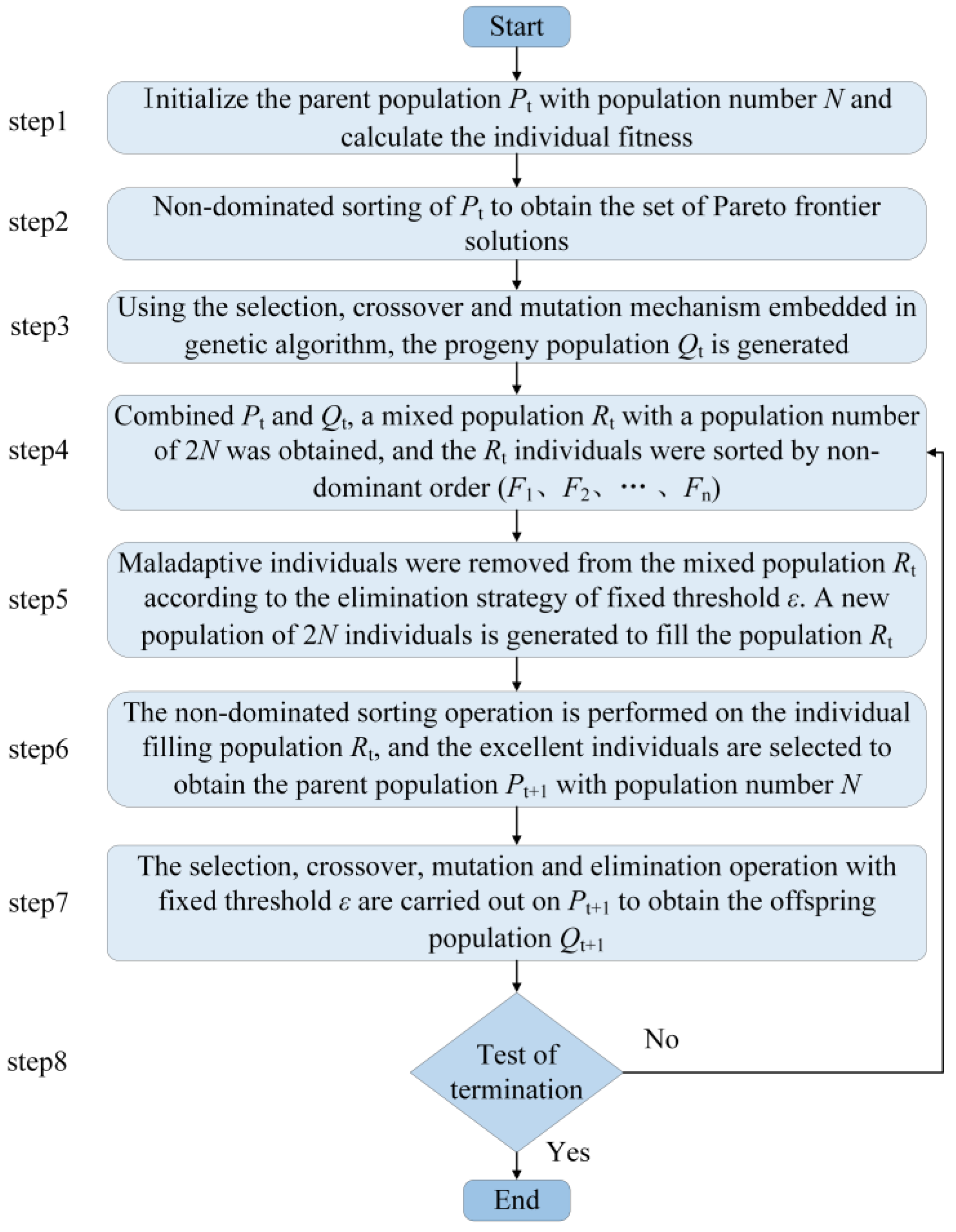
5.2.1. Improved NSGA-II Algorithm
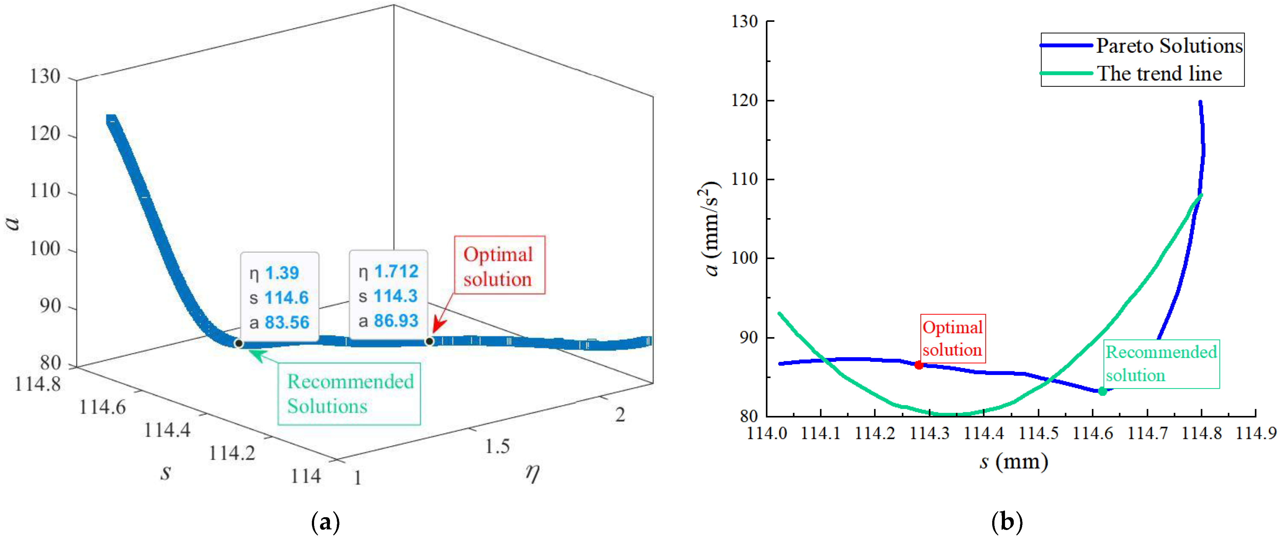
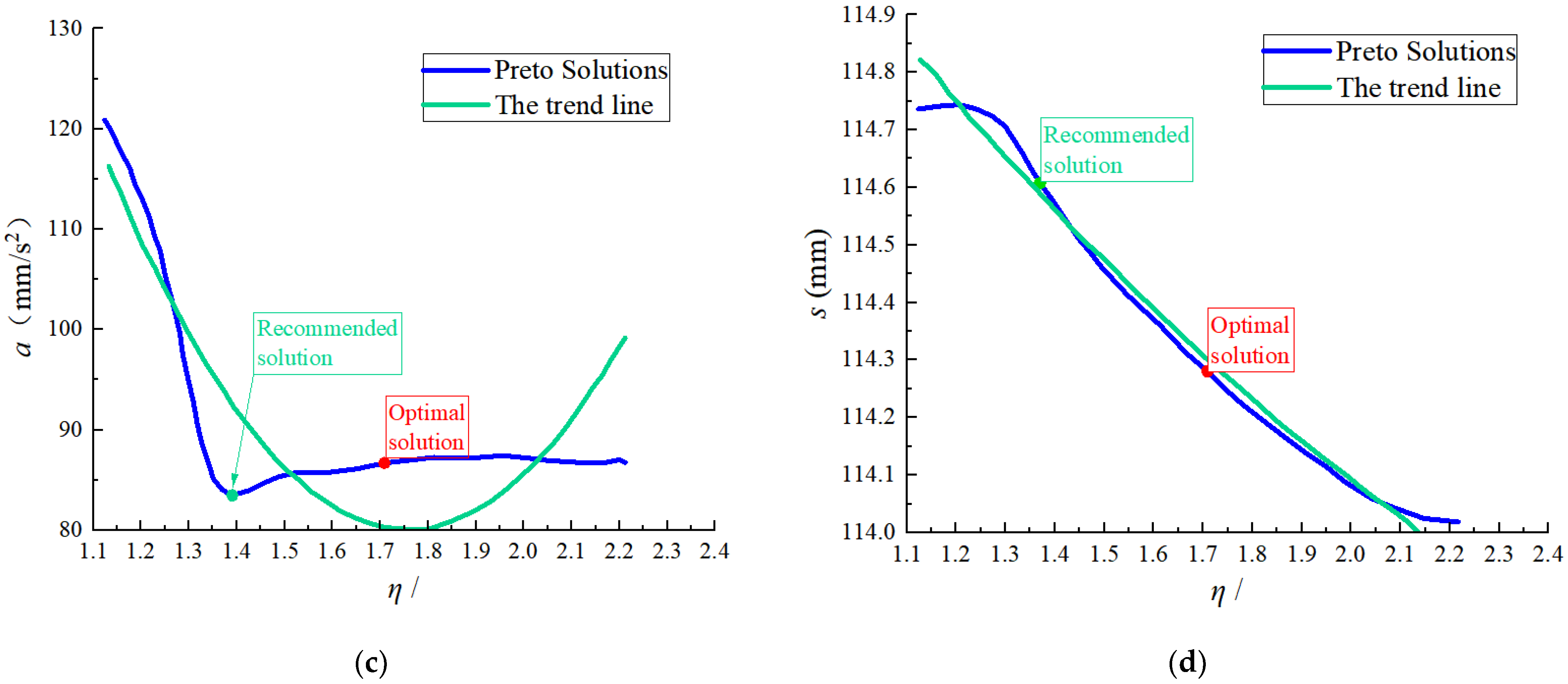
5.2.2. Multi-Objective Optimal Design
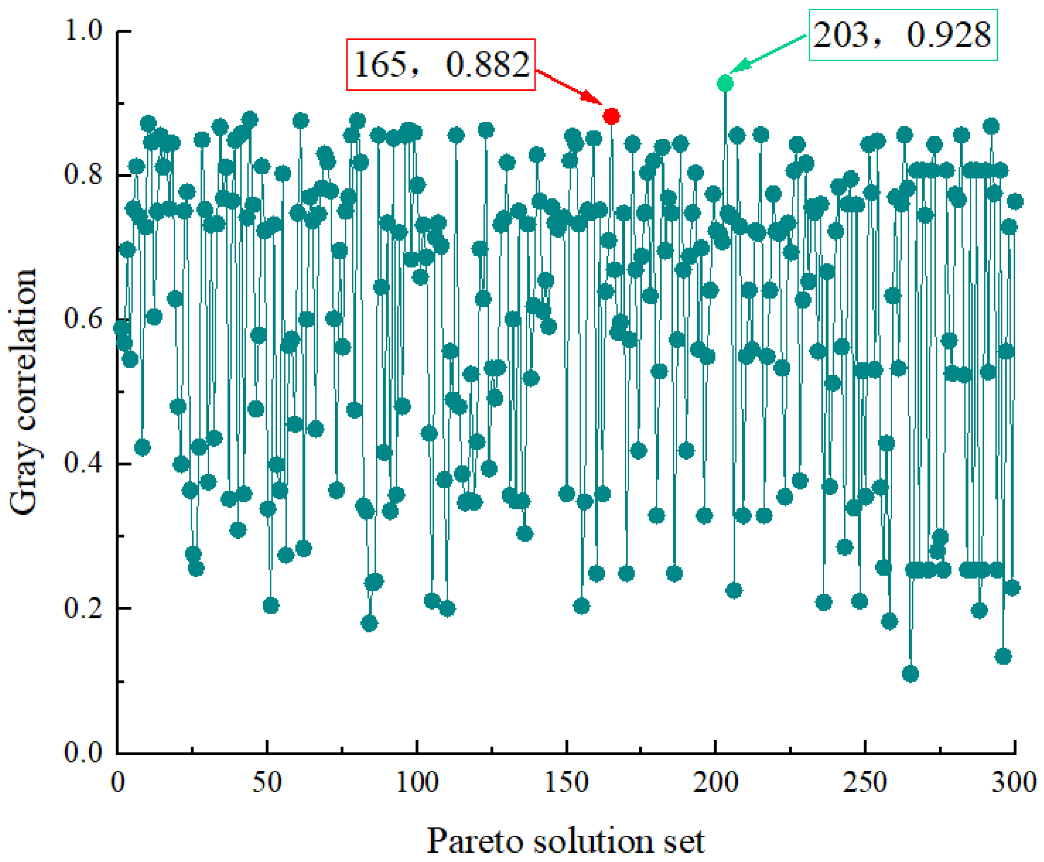
5.3. Entropy-Weighted Gray Correlation Ranking
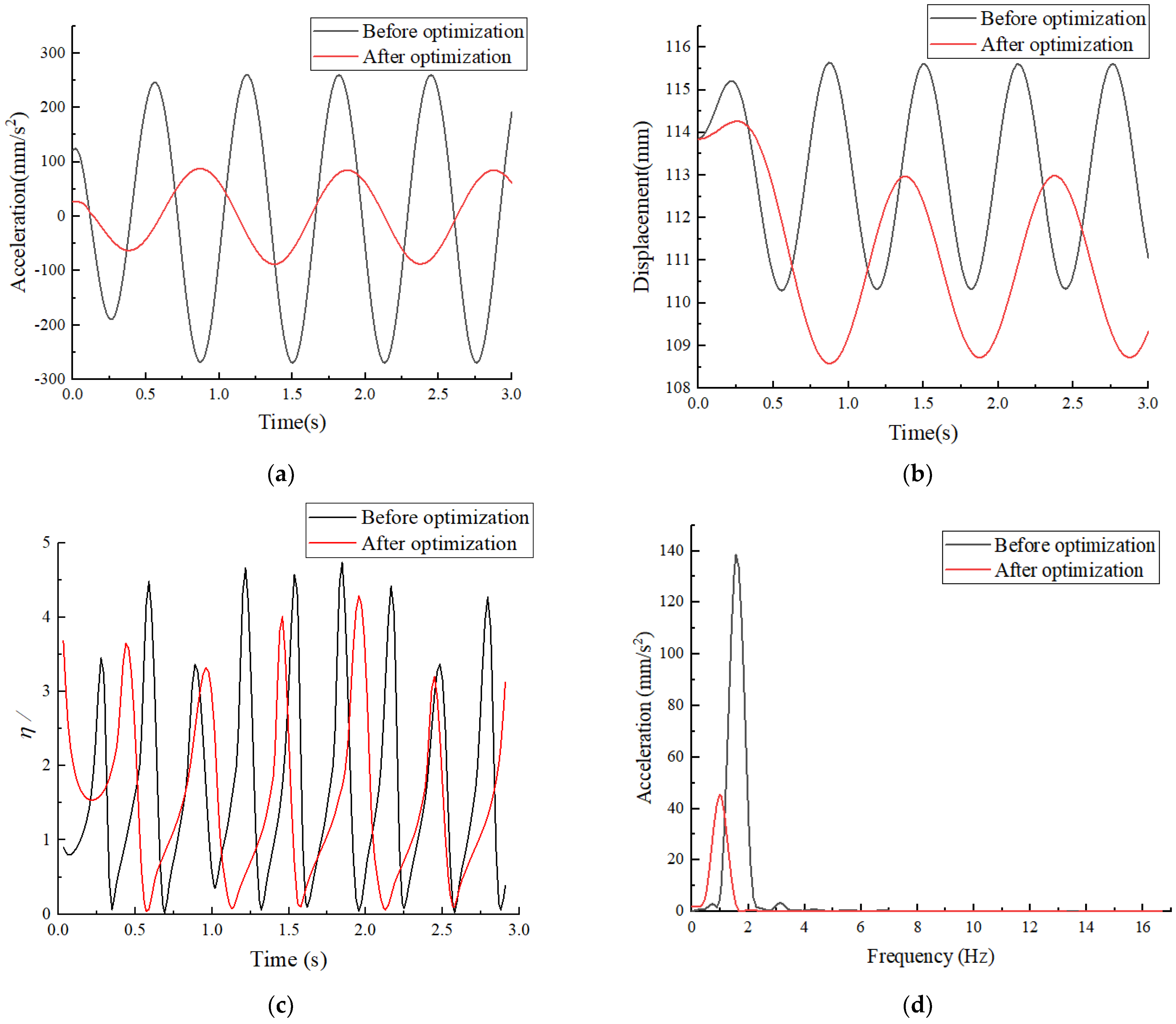
5.4. Comparison of Vibration Vibration Attenuation before and after Optimization
6. Conclusions
- (1)
- The equivalent stiffness and equivalent damping of the seat suspension are derived. The equivalent stiffness is mainly related to the spring stiffness, and the equivalent damping is mainly related to the damper damping. The scissor seat suspension under micro-amplitude vibration conditions can be approximated as a linear vibration system. In the range of values of seat suspension inherent frequency and damping ratio , the larger the seat suspension load mass, the larger the vibration amplitude of the seat on the vibration amplification zone and the greater the vibration attenuation in the vibration isolation zone. When the seat suspension load mass increased by 55.56% and 88.89%, the seat natural frequency decreased by 20.20% and 27.27%, the damping ratio decreased by 22.86% and 28.57%, and the seat vibration peak increased by 5.37% and 13.42%.
- (2)
- Within the constraint range of seat suspension inherent frequency and damping ratio : under the condition of certain value of damper damping, as the value of spring stiffness increases, the value of acceleration and displacement of seat upper plane response increases, and the vibration attenuation ability of seat decreases. Under the condition of a certain value of spring stiffness, as the value of damper damping increases, the value of acceleration and displacement of seat upper plane response decreases, and the vibration attenuation of seat suspension improves.
- (3)
- Through main effect analysis and contribution analysis, the relationship between the control variable and response index is obtained. The effect of k on the response to a and s is decisive, and the effect of c on the response from a and s is second. c on the response to η is decisive, and the effect of k on the response of η is second.
- (4)
- RBF proxy model is constructed by combining experimental design sampling. Based on MNSGA-II multi-objective optimization algorithm, multi-objective optimization of seat suspension vibration performance is conducted, and Pareto frontier disaggregation is obtained. The entropy-weighted gray correlation ranking method is used to obtain the preferred solution that satisfies the range of variables. The effectiveness of the multi-objective optimization in this paper is verified by simulation analysis, and the response indexes a, s, and η vibration attenuation are improved by 66.41%, 2.31%, and 8.19%, respectively, which effectively improves the seat suspension vibration attenuation. The method used in this paper provides a reference for the study of vibration attenuation control of seat suspension.
Author Contributions
Funding
Institutional Review Board Statement
Data Availability Statement
Conflicts of Interest
References
- Rahman, A.; Ali, R.; Kabir, S.N.; Rahman, M.; Al Mamun, R.; Hossen, A. Agricultural Mechanization in Bangladesh: Status and Challenges towards Achieving the Sustainable Development Goals (SDGs). Ama-Agric. Mech. Asia Afr. Lat. Am. 2020, 51, 106–120. [Google Scholar]
- Chen, Y.C.; Chen, L.W.; Chang, M.Y. A Design of an Unmanned Electric Tractor Platform. Agriculture 2022, 12, 112. [Google Scholar] [CrossRef]
- Mano, Y.; Takahashi, K.; Otsuka, K. Mechanization in land preparation and agricultural intensification: The case of ricefrmng in the Cote d’Ivoire. Agric. Econ. 2020, 51, 899–908. [Google Scholar] [CrossRef]
- Brunetti, J.; D’Ambrogio, W.; Fregolent, A. Analysis of the Vibrations of Operators’ Seats in Agricultural Machinery Using Dynamic Substructuring. Appl. Sci. 2021, 11, 4749. [Google Scholar] [CrossRef]
- Han, H.-W.; Dae, K.K.; Hong, I.W.; Man, K.J.; Je, C.S.; Young-Jun, P. Analysis on Whole-Body Vibration of 100 kW Class Agricultural Tractor Operator for Evaluating Ride Comfort. J. Agric. Life Sci. 2022, 56, 135–142. [Google Scholar] [CrossRef]
- Li, Z.; Li, X.; Liu, B.; Wang, J. Influence of vehicle body vibration induced by road excitation on the performance of a vehicle-mounted piezoelectric-electromagnetic hybrid energy harvester. Smart Mater. Struct. 2021, 30, 55019. [Google Scholar] [CrossRef]
- Jung, H.; Park, G.; Kim, J.K. Piezoelectric-based dither control for automobile brake squeal suppression under various braking conditions. J. Vib. Control. 2021, 27, 2192–2204. [Google Scholar] [CrossRef]
- Huang, Y.; Tong, S.; Tong, Z.; Cong, F. Signal Identification of Gear Vibration in Engine-Gearbox Systems Based on Auto-Regression and Optimized Resonance-Based Signal Sparse Decomposition. Sensors 2021, 21, 1868. [Google Scholar] [CrossRef]
- Adam, S.A.; Jalil, N.A.; Rezali, K.M.; Ng, Y.G.; Sound and Vibration Research Group. The effect of posture and vibration magnitude on the vertical vibration transmissibility of tractor suspension system. Int. J. Ind. Ergon. 2020, 80, 103014. [Google Scholar] [CrossRef]
- Yoo, H.; Oh, J.; Chung, W.-J.; Han, H.-W.; Kim, J.-T.; Park, Y.-J.; Park, Y. Measurement of stiffness and damping coefficient of rubber tractor tires using dynamic cleat test based on point contact model. Int. J. Agric. Biol. Eng. 2021, 14, 157–164. [Google Scholar] [CrossRef]
- Oh, J.; Chung, W.J.; Han, H.W.; Kim, J.T.; Son, G.H.; Park, Y.J. Evaluation of Tractor Ride Vivrations by Cab Suspension System. Trans. Asabe 2020, 63, 1465–1476. [Google Scholar] [CrossRef]
- Desai, R.; Guha, A.; Seshu, P. A comparison of different models of passive seat suspensions. Proc. Inst. Mech. Eng. Part D-J. Automob. Eng. 2021, 235, 2585–2604. [Google Scholar] [CrossRef]
- Gao, P.; Liu, H.; Xiang, C.; Yan, P. Vibration reduction performance of an innovative vehicle seat with a vibration absorber and variable damping cushion. Proc. Inst. Mech. Eng. Part D-J. Automob. Eng. 2022, 236, 689–708. [Google Scholar] [CrossRef]
- Cvetanovic, B.; Cvetković, D.; Praščević, M.; Cvetković, M.; Pavlović, M. An analysis of the impact of agricultural tractor seat cushion materials to the level of exposure to vibration. J. Low Freq. Noise Vib. Act. Control. 2017, 36, 116–123. [Google Scholar] [CrossRef] [Green Version]
- Zhu, Z.; Yang, Y.; Wang, D.; Cai, Y.; Lai, L. Energy Saving Performance of Agricultural Tractor Equipped with Mechanic-Electronic-Hydraulic Powertrain System. Agriculture 2022, 12, 436. [Google Scholar] [CrossRef]
- Liao, X.; Du, X.; Li, S. Design of cab seat suspension system for construction machinery based on negative stiffness structure. Adv. Mech. Eng. 2021, 13, 16878140211044931. [Google Scholar] [CrossRef]
- Du, X.M.; Yu, M.; Fu, J.; Peng, Y.X.; Shi, H.F.; Zhang, H. H control for a semi-active scissors linkage seat suspension with magnetorheological damper. J. Intell. Mater. Syst. Struct. 2019, 30, 708–721. [Google Scholar] [CrossRef]
- Deng, L.; Sun, S.; Christie, M.; Li, W. Numerical Study of Rotary Magnetorheological Seat Suspension on the Impact Protection. Adv. Appl. Nonlinear Dyn. Vib. Control. 2021, 2022, 1003–1017. [Google Scholar]
- Zhang, X.; Wang, C.; Guo, K.; Sun, M.; Yao, Q. Dynamics modeling and characteristics analysis of scissor seat suspension. J. Vib. Control. 2017, 23, 2819–2829. [Google Scholar] [CrossRef]
- Deng, L.; Sun, S.; Christie, M.; Ning, D.; Jin, S.; Du, H.; Zhang, S.; Li, W. Investigation of a seat suspension installed with compact variable stiffness and damping rotary magnetorheological dampers. Mech. Syst. Signal Process. 2022, 171, 108802. [Google Scholar] [CrossRef]
- Zhao, Y.; Alashmori, M.; Bi, F.; Wang, X. Parameter identification and robust vibration control of a truck driver’s seat system using multi-objective optimization and genetic algorithm. Appl. Acoust. 2021, 173, 107697. [Google Scholar] [CrossRef]
- Maciejewski, I.; Blazejewski, A.; Pecolt, S.; Krzyzynski, T. A sliding mode control strategy for active horizontal seat suspension under realistic input vibration. J. Vib. Control. 2022, 0, 10775463221082716. [Google Scholar] [CrossRef]
- He, S.; Chen, K.; Xu, E.; Wang, W.; Jiang, Z. Commercial Vehicle Ride Comfort Optimization Based on Intelligent Algorithms and Nonlinear Damping. Shock. Vib. 2019, 2019, 2973190. [Google Scholar] [CrossRef]
- Deng, H.; Deng, J.; Yue, R.; Han, G.; Zhang, J.; Ma, M.; Zhong, X. Design and verification of a seat suspension with variable stiffness and damping. Smart Mater. Struct. 2019, 28, 65015. [Google Scholar] [CrossRef]
- Ning, D.; Du, H.; Sun, S.; Zheng, M.; Li, W.; Zhang, N.; Jia, Z. An Electromagnetic Variable Stiffness Device for Semiactive Seat Suspension Vibration Control. IEEE Trans. Ind. Electron. 2020, 67, 6773–6784. [Google Scholar] [CrossRef]
- Desai, R.; Guha, A.; Seshu, P. Modelling and simulation of an integrated human-vehicle system with non-linear cushion contact force. Simul. Model. Pract. Theory 2021, 106, 102206. [Google Scholar] [CrossRef]
- Jiang, R.; Jin, Z.; Ci, S.; Liu, D.; Sun, H. Reliability-based multilevel optimization of carbon fiber reinforced plastic control arm. Struct. Multidiscip. Optim. 2022, 65, 314. [Google Scholar] [CrossRef]
- Jiang, R.; Jin, Z.; Liu, D.; Wang, D. Multi-Objective Lightweight Optimization of Parameterized Suspension Components Based on NSGA-II Algorithm Coupling with Surrogate Model. Machines 2021, 9, 107. [Google Scholar] [CrossRef]
- Jiang, R.; Sun, T.; Liu, D.; Pan, Z.; Wang, D. Multi-Objective Reliability-Based Optimization of Control Arm Using MCS and NSGA-II Coupled with Entropy Weighted GRA. Appl. Sci. 2021, 11, 5825. [Google Scholar] [CrossRef]
- Pandey, M.; Regis, R.G.; Datta, R.; Bhattacharya, B. Surrogate-assisted multi-objective optimization of the dynamic response of a freight wagon fitted with three-piece bogies. Int. J. Rail Transp. 2021, 9, 290–309. [Google Scholar] [CrossRef]
- Yang, L.; Wang, R.; Sun, Z.; Meng, X.; Zhu, Z. Multi-objective optimization design of hydropneumatic suspension with gas-oil emulsion for ride comfort and handling stability of an articulated dumper truck. Eng. Optim. 2021, 24, 1–20. [Google Scholar] [CrossRef]
- Grotti, E.; Mizushima, D.M.; Backes, A.D.; Awruch, M.D.D.F.; Gomes, H.M. A novel multi-objective quantum particle swarm algorithm for suspension optimization. Comput. Appl. Math. 2020, 39, 105. [Google Scholar] [CrossRef]
- Zhao, Y.; Xu, H.; Deng, Y.; Wang, Q. Multi-objective optimization for ride comfort of hydro-pneumatic suspension vehicles with mechanical elastic wheel. Proc. Inst. Mech. Eng. Part D-J. Automob. Eng. 2019, 233, 2714–2728. [Google Scholar] [CrossRef]
- Prasad, V.; Pawaskar, D.N.; Seshu, P. Controller design and multi-objective optimization of heavy goods vehicle suspension system by geometry-inspired GA. Struct. Multidiscip. Optim. 2021, 64, 89–111. [Google Scholar] [CrossRef]
- Hua, Y.; Zhu, H.; Xu, Y. Multi-Objective Optimization Design of Bearingless Permanent Magnet Synchronous Generator. IEEE Trans. Appl. Supercond. 2020, 30, 1–5. [Google Scholar] [CrossRef]
- Varela, M.; Gyi, D.; Mansfield, N.; Picton, R.; Hirao, A.; Furuya, T. Engineering movement into automotive seating: Does the driver feel more comfortable and refreshed? Appl. Ergon. 2019, 74, 214–220. [Google Scholar] [CrossRef] [Green Version]
- Nagarkar, M.P.; Patil, G.J.V.; Patil, R.N.Z. Optimization of nonlinear quarter car suspension-seat-driver model. J. Adv. Res. 2016, 7, 991–1007. [Google Scholar] [CrossRef] [Green Version]
- Kim, J.H.; Dennerlein, J.T.; Johnson, P.W. The effect of a multi-axis suspension on whole body vibration exposures and physical stress in the neck and low back in agricultural tractor applications. Appl. Ergon. 2018, 68, 80–89. [Google Scholar] [CrossRef]
- Kim, J.H.; Marin, L.S.; Dennerlein, J.T. Evaluation of commercially available seat suspensions to reduce whole body vibration exposures in mining heavy equipment vehicle operators. Appl. Ergon. 2018, 71, 78–86. [Google Scholar] [CrossRef]
- Liu, P.; Ning, D.; Luo, L.; Zhang, N.; Du, H. An Electromagnetic Variable Inertance and Damping Seat Suspension with Controllable Circuits. IEEE Trans. Ind. Electron. 2022, 69, 2811–2821. [Google Scholar] [CrossRef]
- Zheng, E.; Fan, Y.; Zhu, R.; Zhu, Y.; Xian, J. Prediction of the vibration characteristics for wheeled tractor with suspended driver seat including air spring and MR damper. J. Mech. Sci. Technol. 2016, 30, 4143–4156. [Google Scholar] [CrossRef]
- Zhang, S.; Liu, K.; Zhang, S.; Xu, L. Study on Aerodynamic Performance and Lightweight Multiobjective Optimization Design of Wheel With Entropy Weighted Grey Relational Analysis Methods. IEEE Access 2022, 10, 93421–93438. [Google Scholar] [CrossRef]
- Mehta, C.R.; Tewari, V.K. Biomechanical model to predict loads on lumbar vertebra of a tractor operator. Int. J. Ind. Ergon. 2015, 47, 104–116. [Google Scholar] [CrossRef]
- Yi-jie, S.H.U.I.; Rakheja, S.; Shangguan, W.B. Calculation and analysis for equivalent stiffness and damping of a scissor type seat-seat suspension-human body system. J. Vib. Shock. 2016, 35, 38–44. [Google Scholar]
- Verma, S.; Pant, M.; Snasel, V. A Comprehensive Review on NSGA-II for Multi-Objective Combinatorial Optimization Problems. IEEE Access 2021, 9, 57757–57791. [Google Scholar] [CrossRef]


| /mm | /mm | /mm | /mm | /mm | /(°) | /(°) | /(°) |
|---|---|---|---|---|---|---|---|
| 50 | 132 | 107 | 132 | 120 | 115 | 20.6 | 11.6 |
| Load Capacity of Different Suspensions/kg | Vibration Transfer Function Peak Frequency/Hz | Vibration Transfer Function Peak Amplitude/mm | Inherent Frequency/Hz | Damping Ratio | Vibration Transmission Rate at 3 Hz |
|---|---|---|---|---|---|
| m = 45 | 1.78 | 2.98 | 1.98 | 0.35 | 0.87 |
| m = 70 | 1.28 | 3.14 | 1.58 | 0.27 | 0.51 |
| m = 85 | 1.00 | 3.38 | 1.44 | 0.25 | 0.41 |
| Different Stiffnesses k/(N/mm) | Maximum Response Acceleration/(mm/s2) | Maximum Response Displacement/mm | Vibration Transmission Rate | Seat Suspension Inherent Frequency/Hz |
|---|---|---|---|---|
| k = 70 | 87.02 | 114.48 | 1.708 | 1.01 |
| k = 170 | 255.12 | 115.61 | 1.336 | 1.58 |
| k = 272 | 469.13 | 116.39 | 1.083 | 1.99 |
| Different Damping c/(N⋅s/mm) | Maximum Response Acceleration/(mm/s2) | Maximum Response Displacement/mm | Vibration Transmission Rate | Seat Suspension Inherent Frequency/Hz |
|---|---|---|---|---|
| c = 1.9 | 352.05 | 116.58 | 1.228 | 1.59 |
| c = 3.7 | 248.36 | 115.52 | 1.043 | 1.59 |
| c = 5.5 | 223.19 | 115.22 | 1.272 | 1.59 |
| Main Effect Evaluation Indicators | Acceleration a/(mm/s2) | Displacement s/mm | Transmission Rate/ | |||||
|---|---|---|---|---|---|---|---|---|
| k | c | k | c | k | c | |||
| Level | 1 | 128.964 | 391.331 | 114.821 | 116.650 | 1.853 | 3.651 | |
| 2 | 182.668 | 235.396 | 115.262 | 115.451 | 1.902 | 2.294 | ||
| 3 | 252.884 | 302.738 | 115.684 | 115.674 | 2.251 | 2.062 | ||
| 4 | 335.443 | 215.925 | 116.062 | 115.322 | 2.420 | 1.671 | ||
| 5 | 464.419 | 218.989 | 116.561 | 115.310 | 2.803 | 1.541 | ||
| The main Effect value | 335.455 | 175.406 | 1.740 | 1.340 | 0.950 | 2.110 | ||
| Sorting | 1 | 2 | 1 | 2 | 1 | 2 | ||
| Interaction effect value | 132.672 | 0.580 | 0.705 | |||||
| The overall average | 272.88 | 115.68 | 2.24 | |||||
| No. | Design Variables | Performance Response | |||
|---|---|---|---|---|---|
| k(N/mm) | c(N⋅s/mm) | a(mm/s2) | s(mm) | η | |
| 1 | 95.055 | 4.394 | 119.380 | 114.930 | 1.449 |
| 2 | 261.120 | 3.403 | 442.620 | 116.310 | 2.457 |
| 3 | 264.008 | 3.403 | 442.620 | 116.310 | 2.457 |
| … | … | … | … | … | … |
| 79 | 73.990 | 4.694 | 104.120 | 114.810 | 1.323 |
| 80 | 258.415 | 1.648 | 712.660 | 118.200 | 4.718 |
| Performance Response | Kriging Surrogate Model | RBF Surrogate Model |
|---|---|---|
| R2 | R2 | |
| a/(mm/s2) | 0.9851 | 0.9921 |
| s/mm | 0.9624 | 0.9772 |
| η/ | 0.9773 | 0.9928 |
| / | 0.9835 | 0.9932 |
| No. | Number of Gray Correlations for Each Response Index | Gray Correlation | Sort by | ||
|---|---|---|---|---|---|
| a(mm/s2) | s(mm) | η | |||
| 1 | 0.516 | 0.667 | 0.632 | 0.589 | 179 |
| 2 | 0.524 | 0.560 | 0.692 | 0.568 | 186 |
| … | … | … | … | … | … |
| 165 | 0.926 | 0.887 | 0.763 | 0.882 | 2 |
| … | … | … | … | … | … |
| 203 | 0.967 | 0.896 | 0.876 | 0.928 | 1 |
| … | … | … | … | … | … |
| 300 | 0.763 | 0.853 | 0.634 | 0.764 | 82 |
| Vibration Performance Parameters | k/(N/mm), c/(N⋅s/mm) Before and After Optimization | Performance Improvement Rate/% | |
|---|---|---|---|
| k = 172.28, c = 3.37 | k = 68.36, c = 2.77 | ||
| Maximum response acceleration/(mm/s2) | 259 | 87 | 66.41 |
| Maximum response displacement/(mm) | 115.64 | 112.97 | 2.31 |
| Rate of vibration transmission/ | 1.257 | 1.360 | 8.19 |
| Seat suspension inherent frequency/Hz | 1.56 | 1.00 | 35.90 |
Disclaimer/Publisher’s Note: The statements, opinions and data contained in all publications are solely those of the individual author(s) and contributor(s) and not of MDPI and/or the editor(s). MDPI and/or the editor(s) disclaim responsibility for any injury to people or property resulting from any ideas, methods, instructions or products referred to in the content. |
© 2022 by the authors. Licensee MDPI, Basel, Switzerland. This article is an open access article distributed under the terms and conditions of the Creative Commons Attribution (CC BY) license (https://creativecommons.org/licenses/by/4.0/).
Share and Cite
Zhang, S.; Wei, W.; Chen, X.; Xu, L.; Cao, Y. Vibration Performance Analysis and Multi-Objective Optimization Design of a Tractor Scissor Seat Suspension System. Agriculture 2023, 13, 48. https://doi.org/10.3390/agriculture13010048
Zhang S, Wei W, Chen X, Xu L, Cao Y. Vibration Performance Analysis and Multi-Objective Optimization Design of a Tractor Scissor Seat Suspension System. Agriculture. 2023; 13(1):48. https://doi.org/10.3390/agriculture13010048
Chicago/Turabian StyleZhang, Shuai, Weizhen Wei, Xiaoliang Chen, Liyou Xu, and Yuntao Cao. 2023. "Vibration Performance Analysis and Multi-Objective Optimization Design of a Tractor Scissor Seat Suspension System" Agriculture 13, no. 1: 48. https://doi.org/10.3390/agriculture13010048