Article

Comparison of Shuttleworth–Wallace and Dual Crop Coefficient Method for Estimating Evapotranspiration of a Tea Field in Southeast China

1
Research Center of Fluid Machinery Engineering and Technology, Jiangsu University, Zhenjiang 212013, China
2
State Key Laboratory of Hydrology-Water Resources and Hydraulic Engineering, Nanjing Hydraulic Research Institute, Nanjing 210029, China
3
Institute of Agricultural Engineering, Jiangsu University, Zhenjiang 212013, China
4
South Subtropical Crops Research Institute, Chinese Academy of Tropical Agricultural Sciences, Zhanjiang 524091, China
*
Author to whom correspondence should be addressed.
Agriculture 2022, 12(9), 1392; https://doi.org/10.3390/agriculture12091392
Submission received: 14 January 2022 / Revised: 1 March 2022 / Accepted: 1 March 2022 / Published: 5 September 2022
(This article belongs to the Special Issue Water-Saving Irrigation Technology and Strategies for Crop Production)

Abstract

:
Determination of evaporation (E) and transpiration (T) in tea fields separately is important in developing precise irrigation scheduling and enhancing water use efficiency. In this study, the Shuttleworth–Wallace (S-W) model was applied to simulate the variations of E and T based on the data from 2015 to 2018 in a tea field in southeast China. The dual crop coefficient (D-K) method recommended by FAO-56 was also applied to calculate E and T, using the same data set to compare with the S-W model. The measured crop coefficient (Kc) ranged from 0.43 to 1.44 with the average value was 0.90 during 1–150 DOY (days of year), and the measured Kc tended to be stable with the average value of 0.83 during 151–365 DOY in 2015. The S-W model estimated ETc with root mean square error (RMSE) and R2 of 0.45 mm d−1 and 0.97, while for the D-K method the values were 0.61 mm d−1 and 0.95. Therefore, both approaches could estimate the E and T separately in tea fields in southeast China, however, the D-K method had a slightly poorer accuracy compared to the S-W model in the estimation of ETc.

1. Introduction

Tea, as one of the oldest (since 3000 BCE) and most popular nonalcoholic caffeine-containing beverages, has been integrated into the social and daily life in China. At present, tea is commercially cultivated in more than 3.80 million hectares of land on a continent-wide scale, and 5.56 million metric tons of tea world-wide were produced annually in 2014 [1]. Irrigation is essential to ensure tea production in southeast China, and the appropriate amount of irrigation water at the right time directly increases tea quality. However, most of the tea farmers in southeast China are still using an empirically determined irrigation quota due to lack of accurate irrigation basis for tea plants. Therefore, accurate determination of tea evapotranspiration (ETc) is urgently needed to develop precise irrigation scheduling and enhance water use efficiency in this region [2,3].
Single source models, such as the Penman–Monteith (PM) method [4,5] pan evaporation method [6], Takakura method [7] and Priestley–Taylor method [8], are often used to determine ETc for grain crop fields [9]. However, unlike grain crops, tea fields always have wide row space (120 cm) between tea plants so that large soil surface is uncovered by the tea plants. Hence, the above single source ETc models that do not consider independently soil evaporation (E) are especially problematic because the soil evaporation ratio (E/ETc) is large [10]. Many researchers have reported that the soil evaporation (E) should not be neglected in estimating ETc and it accounts for 20–30% of the ETc for a cherry orchard [10], 25% of ETc for greenhouse tomato [11], 17.8–26.4% of ETc for a mulched greenhouse hot pepper [9], and 7.75–21.87% of ETc for greenhouse cucumber [12]. Accordingly, the two source Shuttleworth–Wallace (S-W) model [13] and the dual crop coefficient (D-K) method [14], which can estimate transpiration (T) and E separately, have been validated to estimate ETc in different ecosystems [11,15,16,17,18,19].
The S-W model is the first analytical model, combining T and E by formulating the different media through which evaporative flux travels as resistances [20]. Three aerodynamic resistances among different interface (bulk boundary layer resistance: r a a , aerodynamic resistance between mean canopy flow and reference height: r a c , aerodynamic resistance between soil surface and mean canopy flow: r a s ) are introduced simultaneously to regulate the transfer between these surfaces and the atmosphere [11,21]. Canopy and soil surface resistances ( r s c and r s s ) are introduced simultaneously into the S-W model to regulate the transfer of energy from plants and soil, respectively [11]. Ortega-Farias et al. [22] and Zhao et al. [19] parameterized the S-W model by adopting a Jarvis type r s c formulation and power function between r s s and soil water content at the top layer to estimate vineyard ETc. Zhu et al. [17] parameterized the S-W model by adopting a Leuning type r s c formulation and exponential function between r s s and soil water content to estimate alpine grassland ETc on the Qinghai–Tibetan plateau. Huang et al. [12] parameterized the S-W model based on the measured stomatal resistance and E, by adopting an exponential function between r s c and net radiation and a power function between r s s and soil water content to estimate cucumber ETc in a Venlo-type greenhouse. Previous studies indicated that the S-W model performed well in estimating ETc of vineyard [19,22,23], paddy field [24], orchard [10,25], greenhouse tomato [11], and maize [26,27], but it is challenging to parameterize the two resistances.
To simplify the parameterization process for modeling T and E separately, the Food and Agricultural Organization of the United Nations (FAO) developed an indirect method, named dual crop coefficient (D-K) method, to estimate ETc [14]. The D-K method, allows the separation of E and T and divides crop coefficient (Kc) into basal crop coefficient (Kcb) and soil evaporation coefficient (Ke) [11,19]. Due to its practical simplicity, the D-K method is widely adopted to estimate ETc in different types of sparse crops and climatic regions [26]. Despite the increasing relevance of using the D-K method for modeling crop ETc, determination of Kcb and Ke is challenging [28]. The straightforward adoption of generalized Kcb recommended by FAO-56 can lead to errors in the estimation of ETc and its components, because the dividing of crop growth period and associated crop coefficients are closely related to local climate and crop condition [19]. Zhao et al. [29] observed Kcb for maize were 0.20, 1.10, and 0.45 (at the initial, mid, and end stage), respectively, in the semiarid to sub-humid climate of the North China Plain. Contrastingly, Miao et al. [30] reported that observed Kcb for maize were 0.10, 1.15, and 0.25 (at the initial, mid, and end stage), respectively, in the desert climate of the Hetao irrigation district. Rosa et al. [31] also reported the observed Kcb for maize were 0.07, 1.15, and 0.20 (at the initial, mid, and end stage), respectively, in the dry sub-humid climate of southern Portugal.
While previous studies have reported that the S-W and D-K methods had different performances for various crops grown in different regions, no study has been conducted to assess and compare the performances of the S-W and D-K methods for estimating ETc for perennial plants like tea in southeast China. Therefore, the purpose of this study was to (1) parameterize the resistances and coefficients of soil-atmosphere and plant-atmosphere interface of the S-W and D-K model based on detailed meteorological data from a tea field in southeast China; (2) compare and evaluate the performances of the S-W and D-K method in estimating ETc based on the measured ETc by Bowen ratio energy balance method, so as to provide accurate estimation of ETc for tea fields in southeast China.

2. Materials and Methods

2.1. Field Observation

The experiment was conducted in a tea field located at Jiangsu province, China (31°65′ N, 119°23′ E, 23 m a.s.l) from 2015 to 2018. The experiment site is located in a subtropical monsoon climate, average annual precipitation is 1058.8 mm, and about 750 mm occurs in spring and summer; mean, maximum, and minimum air temperatures through the year are 15.2 °C, 36.6 °C, and −5.7 °C, respectively. The soil text in the study area is medium loam and the field capacity is 28% [32].
Anji White tea, which is one of the cultivars of tea in China, was used for the experiment. The size of the observation field was 55 × 58 m and was surrounded by other tea fields, with the total area larger than 7000 m2 [32]. The tea plants were transplanted into the field on 5 March 2014, with 120 cm spacing between the rows, and 52 cm spacing within a row. According to the FAO-56 and the actual measurements of the tea plants, the period from transplanting to the end of 2018 was seen as the initial growing stage of the tea plants, and the average leaf area index (LAI) was around 2.5.
The latent heat flux of tea field was measured by a Bowen ratio energy balance system installed in the center of field. The system consists of two layers of high-accuracy temperature and humidity sensors, radiometers, a soil heat flux plate, a three-cup anemometer, a solar power supply equipment, and a data logger. Two layers (1.5 and 2.0 m above the ground surface) of air temperature (Ta) and relative humidity (RH) were measured with sensors HMP155A (Vaisala, Finland) with high measurement accuracies (±0.2 °C from −10 to 40 °C for Ta, ± 1 % from 0 to 90 % for RH). The absolute error between the two HMP155A sensors was calibrated by setting them at the same height before the field observation. The radiometers (CNR-4, Kipp and Zonen, Amsterdam, The Netherland), which can measure downward shortwave/longwave and upward shortwave/longwave radiation separately, were installed at 2.5 m above the ground. The calculations of longwave radiation components were corrected as a thermal effect caused by instrument heating. Soil heat flux was measured at 2 cm depth with a soil heat plate HFP01-L10 (Campbell Scientific, Logan, UT, USA). Wind speed was measured with a three-cup anemometer A100L2 (MetOne, New York, NY, USA) at 2.0 m above the ground. Soil volumetric water content and soil temperature were measured by Hydra Probe sensors by setting the sensors at five different depths within the soil layer (5, 10, 20, 50, and 70 cm). All the data were obtained every 1 s and recorded by a data logger CR3000-NB (Campbell Scientific, USA). Due to some technical problems, the data 335-356 days of year (DOY) in 2016 and 193-300 DOY in 2017 were lost.
In this study, the direction of the prevailing winds during the growing season were westerly, the influence of fetch was not considered due to the similar coverage, and the irrigation intensity for 200 m of upwind direction of the observation field [32].

2.2. Bowen Ratio Energy Balance Method

The latent heat flux can be determined by the Bowen ratio energy balance method as follows:
LE = R n     G 1 + β
β = γ   Δ T Δ e
where LE is the latent heat flux (W m−2), Rn the net radiation (W m−2), G is the ground heat flux (W m−2), the ΔT and Δe are the temperature (°C) and vapor pressure (kPa) difference between the two measurement layers, respectively, and γ is the psychrometric constant (kPa °C−1).

2.3. Shuttleworth–Wallace (S-W) Model

The evapotranspiration (ETc), tea plants transpiration (T), and soil evaporation (E) can be calculated by the following expressions based on the S-W model [13]:
ET c = T + E
T = C c Δ A + ( ( ρ a c p D Δ r a c A s ) / ( r a a + r a c ) ) Δ + γ ( 1 + ( r s c / ( r a a + r a c ) ) )
E = C s Δ A + ( ( ρ a c p D Δ r a c ( A A s ) ) / ( r a a + r a c ) ) Δ + γ ( 1 + ( r s s / ( r a a + r a s ) ) )
C c = 1 + R c R a R s ( R c + R a ) 1
C s = 1 + R s R a R c ( R s + R a ) - 1
where Cc is canopy resistance coefficient; Cs is soil surface resistance coefficient; Δ is the slope of the saturation vapor pressure curve at temperature (kPa °C1); cp is specific heat of the air at constant pressure (= 1013 J kg1 °C1); ρa is air density (kg m3); D is water vapor pressure deficit (kPa); r s c is the canopy resistance (s m1); r a c is bulk boundary layer resistance of the vegetative elements in the canopy (s m1); r a a is aerodynamic resistance between mean canopy flow and reference height (s m1); r a s is aerodynamic resistance between soil surface and mean canopy flow (s m1); and r s s is soil surface resistance (s m1). The S-W model adopts the concept of a bulk boundary layer resistance, r a c , which controls transfer between the surface of vegetation and the canopy air steam. Vertical transport is controlled by two further aerodynamic resistances ( r a a and r a s ). r a a is the transfer resistance between the hypothetical mean canopy flow and the reference height above the crop. r a s is the aerodynamic resistance encountered by the energy fluxes leaving the substrate before they are incorporated into the mean canopy flow [13]. For simplicity, it is assumed that the various aerodynamic resistances are identical for sensible and latent heat. More detailed approaches that parameterize the three aerodynamic resistances ( r a c , r a a , and r a s ) can be found in [13].
Values of Ra, Rs, and Rc were calculated as follows:
R a = ( Δ + γ ) r a a
R s = Δ + γ r a s + γ r s s
R c = Δ + γ r a c + γ r s c
A and As (W m2) are the available energy leaving the canopy and soil surface, respectively, and were calculated as
A = R n G
A s = R ns G
Rns is net radiation absorbed by soil surface and can be calculated using Beer’s law
R ns = R n   exp ( - C   LAI )
where C is extinction coefficient of the crop for Rn, which was set to 0.7 in this study according to the Lambert–Beer Law [33].

Estimation of Resistances

The canopy resistance ( r s c ) computed from the inversed Equation (4) can be written as Equation (14).
r s c = C C   ( Δ A r a a + r a c + ( ρ a c p D   Δ r a c A s ) ) T   γ Δ r a a + r a c γ r a a   r a c
One approach for modeling r s c , suggested by Katerji and Perrier [34], was established by a relationship between two ratios ( r s c / r a and r * / r a ) [32].
By defining a climatic resistance given as
r * = Δ + γ γ ρ a c p ( e s   e a ) Δ ( R n     G )
A climatic resistance is related to the isothermal resistance and first introduced by Monteith [35] and represents the surface resistance for equilibrium evaporation. The value mainly depends on climatic characteristics, although Rn and G are also influenced by the characteristics of the vegetative surface [36]. Katerji and Perrier [34] presented a linear link between r s c / r a and r * / r a . In this study, we adopted a non-linear functional relationship between r s c / r a and r * / r a presented by Yan et al. [37]
r s c r a = a   ×   r * r a + b   × r * r a + c
The aerodynamic resistance ( r a ) can be calculated from Perrier [38,39]:
r a = ln x d   /   h c d   ln x d   /   z 0 uk 2
where k is the Karman constant (=0.40); x is the reference height (=2 m); hc is the mean crop height (m); d is the zero plane displacement (m); u is the wind speed at the reference height (m/s); and z0 is the roughness length of the crop relative to momentum transfer (m). The z0 and d are defined as 0.63 and 0.13 of the canopy heights, respectively [32].
The soil surface resistance ( r s s ) was calculated using the Ortega-Farias [22] power model, which is expressed as follows:
r s s = 19   ( θ sat θ swc ) 3 . 5
where r s s is soil surface resistance (s m−1); θswc is volumetric soil water content in the top layer of soil at 10 cm depth; θsat is saturated volumetric soil water content at 10 cm depth (0.40 m3 m−3).
In this study, the E was assumed to be negligible during spring shoots with low moisture content in 2015, so the measured T was replaced by the measured LE from March to May in 2015 to parameterize r s c by solving Equation (14). The r s c sub-model was integrated into S-W model for predicting LE and the model’s accuracy was validated by comparing the predicted and measured LE based on the data from 2016 to 2018.

2.4. Dual Crop Coefficient (D-K) Method

In the dual crop coefficient method, the ETc is defined as the product of crop coefficient (Kc) and reference evapotranspiration (ET0), and Kc is divided into soil evaporation coefficient (Ke) and basal crop coefficient (Kcb) [14].
ET c = K c   ×   ET 0
T = K c b   ×   ET 0
E = K e   ×   ET 0

2.4.1. Reference Evapotranspiration

The ASCE-EWRI [40] standardized the PM method for grass reference ET0 with a condensed, simplified form from the original PM method:
ET 0 = 0.408 Δ R n G + γ 900 T a + 273 u ( e s   e a ) Δ + γ ( 1 + 0.34 u )
where ET0 is reference evapotranspiration in mm d−1 for daily time steps, Rn and G are net radiation at the crop surface and soil heat flux density at the soil surface in MJ m2 d1 for daily time steps, and Ta is the daily air temperature at 2.0 m height (°C). The meteorological data in Equation (22) was obtained in the Bowen ratio energy balance system installed in the center of the tea field.

2.4.2. Basal Crop Coefficient (Kcb) and Soil Evaporation Coefficient (Ke)

Based on the FAO-56 [14], Kcb can be expressed as:
K cb = K c   min + ( K cb   full   K c   min   )   ×   1     exp ( 0.7   ×   LAI )
K cb   full = min 1.0 0 + 0.1 h ,   1.2 + 0.04 u   2 0.004 RH min 45 h 3 0.3
where Kc min is the minimum value of basal crop coefficient for bare soil (= 0.1), Kcb full is the basal crop coefficient when crops have nearly full ground cover, h is the tea plant height.
Ke can be expressed as:
K e = K r K c   max K cb     f ew K c   max
K c   max = max 1.2 + 0.04 u 2 0.004 RH min 45 h 3 0.3 , K cb + 0.05
where Kc max is the maximum value of Kc following rain or irrigation, few is the fraction of the soil that is wetted (=0.5) for irrigation, Kr is the evaporation reduction coefficient dependent on the cumulative depth of water depleted from the soil surface, which is expressed as follows [14,41]:
K r = TEW D e TEW REW = 1000 ( θ SWC   0.5 θ wp ) Z e TEW REW
where TEW is total evaporable water (mm), which is the maximum depth of water that can be evaporated from the soil when the soil surface has been initially completely wetted; De is the cumulative depth of evaporation (depletion) from the soil surface layer (mm); REW is the readily evaporable water, which is the maximum depth of water that can be evaporated from the soil surface without restriction; θswc is the actual surface volumetric soil water content and θwp is the surface soil water content at wilting point (=0.12 m3 m3 in this study); Ze is the depth of the surface soil layer that is subject to drying by way of evaporation (=0.10 m in this study).

2.5. Evaluation of Models’ Performance

Statistical indices included a liner regression with 0 interception between observed and simulated values, root mean square error (RMSE), mean absolute error (MAE), index of agreement (d), and Bias were calculated for validating the accuracy of the models:
RMSE = i = 1 N E i O i 2 N
M A E = 1 N i = 1 N E i O i
d =   1 i = 1 N E i O i 2 i = 1 N E i O ¯ + O i O ¯ 2
Bias = i = 1 N ( E i O i ) i = 1 N O i
where N is number of observations, Ei and Oi are estimated and observed values, and O ¯ is the mean observed value, respectively. A perfect model fit will have d = 1 and Bias = 0; positive values of Bias indicate model overestimation, and negative values of Bias indicates model underestimation [9,42].

3. Results

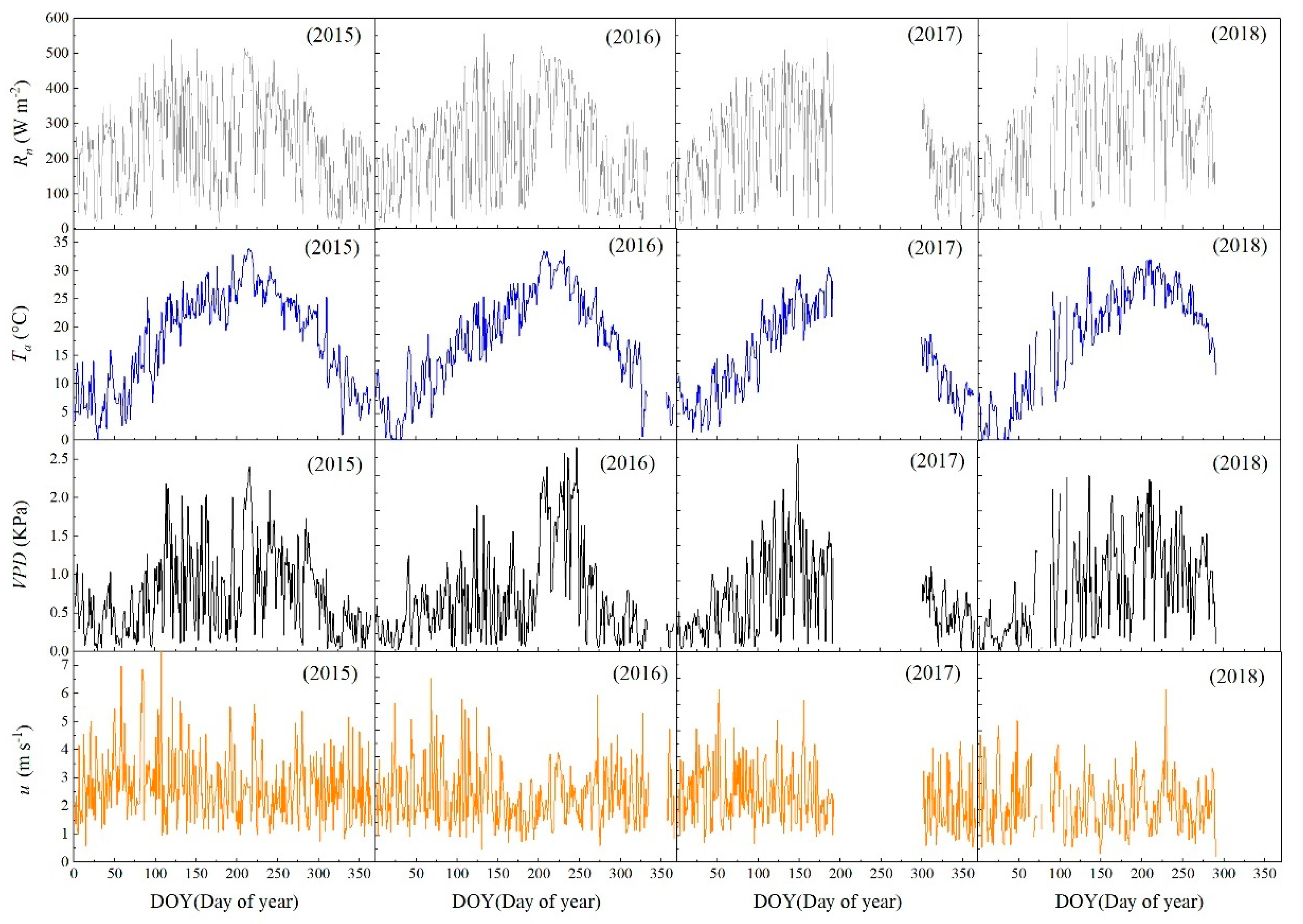
3.1. Interannual Variability of Climatic Factors at the Tea Field

The variations of annual climatic factors (i.e., Rn, Ta, VPD, and u) at the tea field during 2015–2018 are shown in Figure 1. The daytime Rn varied from 0 to 590 W m−2 with an average value of 243, 230, 238, and 290 W m−2 in 2015, 2016, 2017, and 2018, respectively. The daytime air temperature (Ta) changed from −7.1 to 36.1 °C with a mean of 17.9 °C during the four years, while the Ta of 2018 was the highest with a value of 19.6 °C and that of 2017 was the lowest with a value of 15.3 °C. Compared with Ta, VPD showed a similar interannual trend. It had a highest average value of 0.9 kPa in 2018, a minimum average value of 0.7 kPa in 2017 among the four years. The daytime wind speed (u) at height of 2 m varied from 0 to 7.5 m s−1, with an average value of 2.7, 2.4, 2.5, and 2.2 m s−1 in 2015, 2016, 2017, and 2018, respectively.

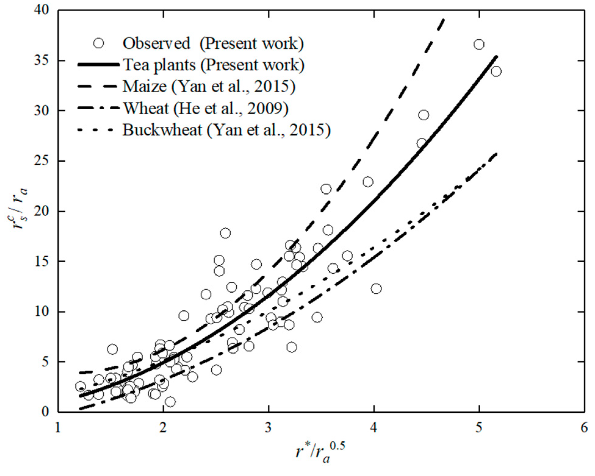
3.2. Parameterization of r s c

Diurnal variation of experimental values of r s c / r a and r * / r a is shown in Figure 2, with a quadratic polynomial relationship being found between r s c / r a and ( r * / r a )0.5. The coefficients a, b, and c in Equation (16) in this study were 1.37, −0.18, and −0.17 (with R2 = 0.84, RMSE = 0.30) for tea plants. Previous studies have been conducted to commonly express r s c / r a and r * / r a as a linear function in alfalfa, grass, maize, and canola fields [34,43,44], but in this study we found a best-fit nonlinear relationship corresponded to a dependence of r s c / r a on the square root of r * / r a . The same function type was also reported in several studies, but the coefficients a, b, and c were different from the presented values (He et al. [45]: wheat field, 0.88, 0.82, and −1.95 in arid regions; Yan et al. [37]: maize field, 2.74, −5.9, and 7.04 in semiarid regions, and buckwheat field, 0.73, 1.25, and −0.28 in humid regions) as shown in Figure 1. As pointed out by Rana et al. [46], the coefficients of those relationships depended on the type of crop, its phenological state, and soil water status. Even for the same crop, the differences in coefficients among studies may exist due to different climatic regions [32,36].

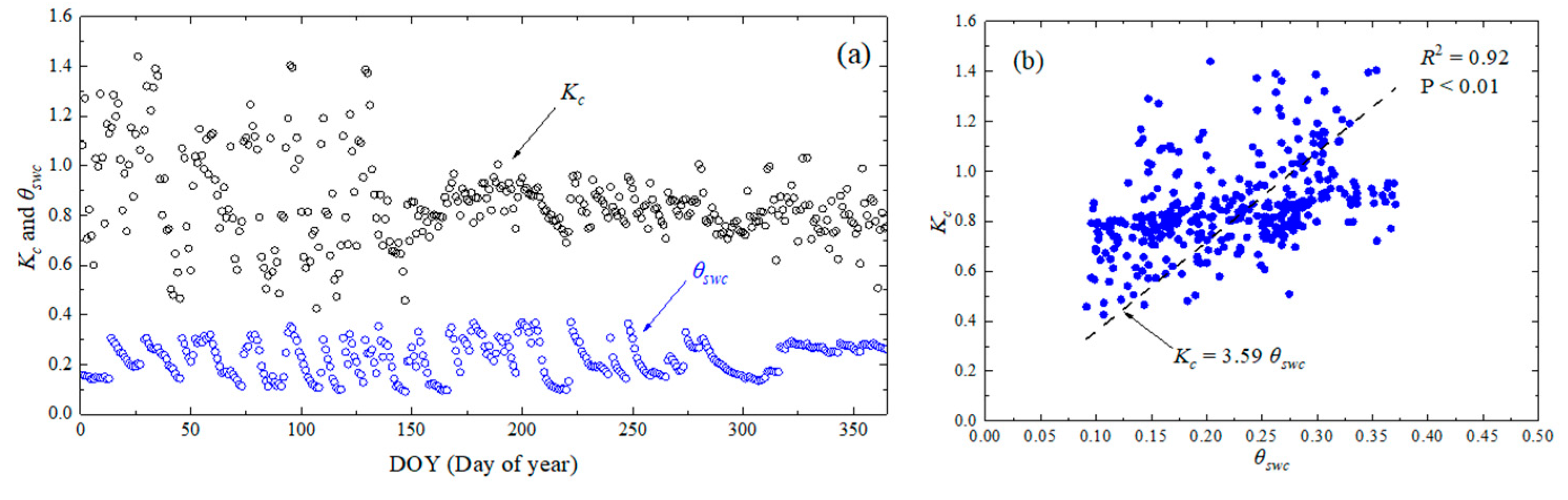
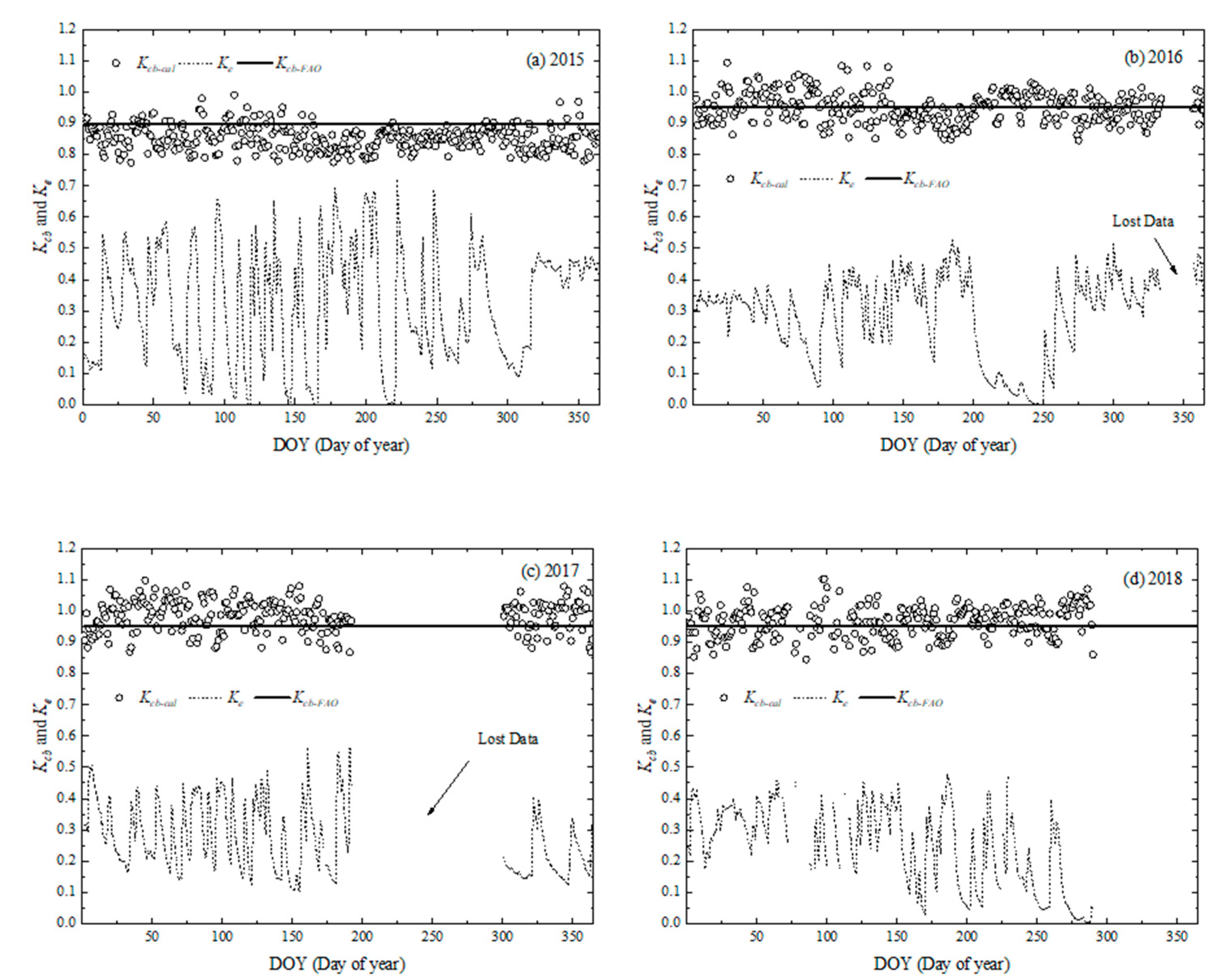
3.3. Crop Coefficient (Kc), Basal Crop (Kcb), and Soil Evaporation Coefficient (Ke)

Figure 3a shows the variations of local measured Kc and the volumetric soil water content (θswc). Both Kc and θswc followed almost the same pattern along with DOY, for which the Kc values ranged from a minimum value of 0.43 in the 107 DOY to a maximum value of 1.44 in the 26 DOY. The measured Kc varied greatly and ranged from 0.43 to 1.44 with an average value of 0.90 during 1–150 DOY, while the Kc tended to be stable with an average value of 0.83 during 151–365 DOY. This may be due to a number of factors, for example; (1) the LAI dramatically changed for collecting tea during the spring and summer seasons; (2) the θswc varied more in the rainy season (Figure 3a), which usually occurred during the spring and summer seasons. Can the local Kc values estimate by the θswc for perennial plants like tea plants? Figure 3b shows the correlation between the local Kc and θswc in 2015, it was surprisingly found that there was a good consistency between the local Kc and θswc (R2 = 0.92, Pearson correlation coefficient = 0.96 and p value = 0.000476 < 0.01).
The calculated basal crop coefficients (Kcb) of tea plants by Equation (23) based on the data from 2015 to 2018 are shown in Figure 4, together with the recommended Kcb by FAO-56 and the soil evaporation coefficient (Ke) calculated by Equation (25). The FAO-56 recommended Kcb for tea plants were 0.90 at initial stages, respectively [14], while the corresponding values of calculated Kcb were 0.89 at the initial stage (2015–2018). Figure 4 shows that the average calculated Kcb was close to, but lower than, the FAO-56 recommended values in 2015, while the average calculated Kcb was 0.95, 0.98, and 0.96 in 2016, 2017, and 2018, close to but more than the FAO-56 recommended values of 0.95. According to Allen et al. [14], Kcb are related to the local conditions, cultural practices, or crop varieties, but local values of Kcb should not be expected to deviate by more than 0.2 from the recommended values. For Ke, it was generally affected by surface soil water content and canopy coverage ratio [47]. The average value of Ke was 0.32 for 2015, higher than the value of 0.28 for 2016, 0.25 for 2017, and 0.23 for 2018, mainly due to the differences in canopy coverage ratio. From the Figure 4, values of Ke were close to 0 during DOY 240–260 in 2016 and DOY 275-285 in 2018, while values of θswc were close to 0 with an average value of 0.04 and 0.07 cm3 cm−3 at the corresponding dates.

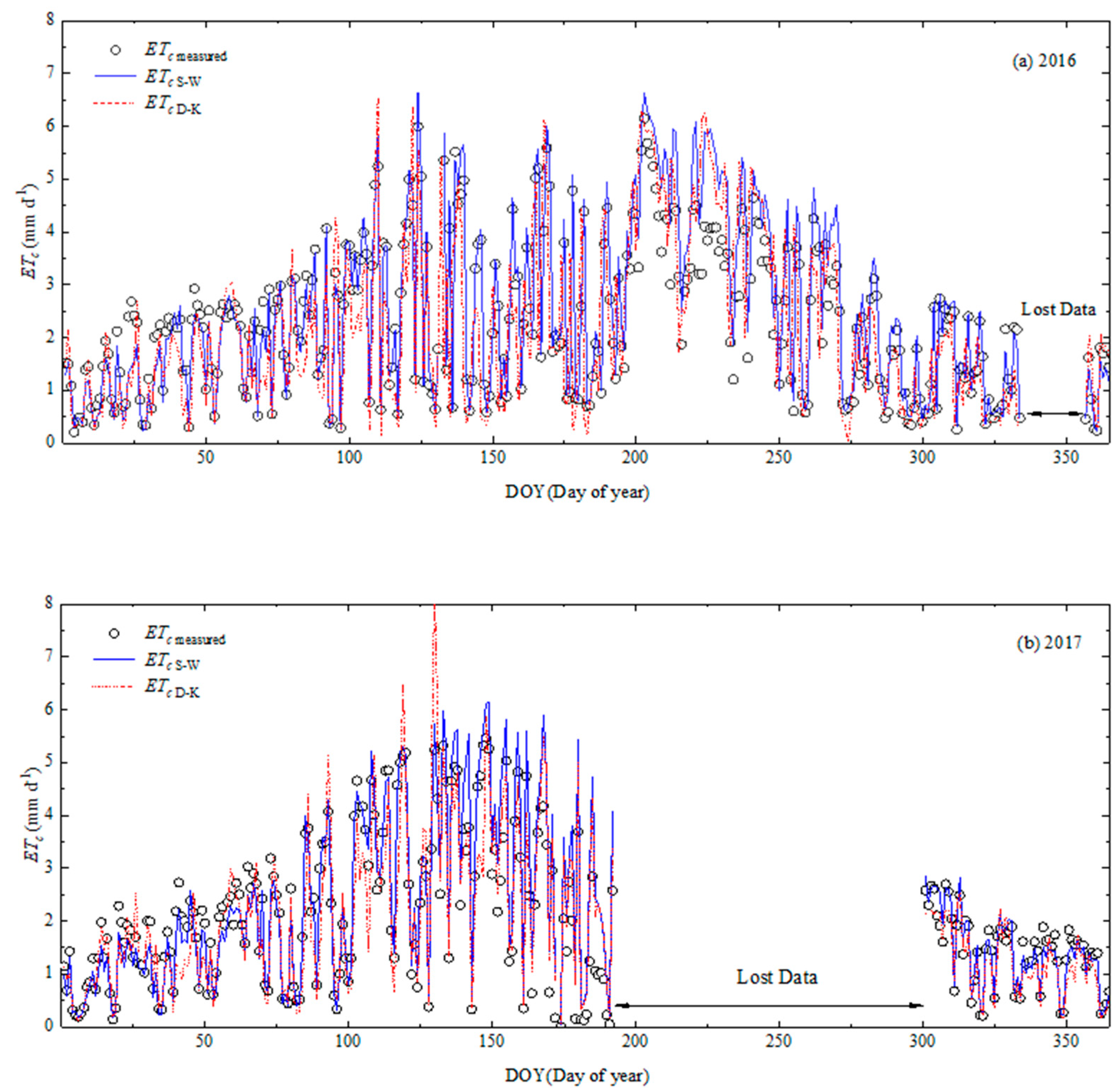
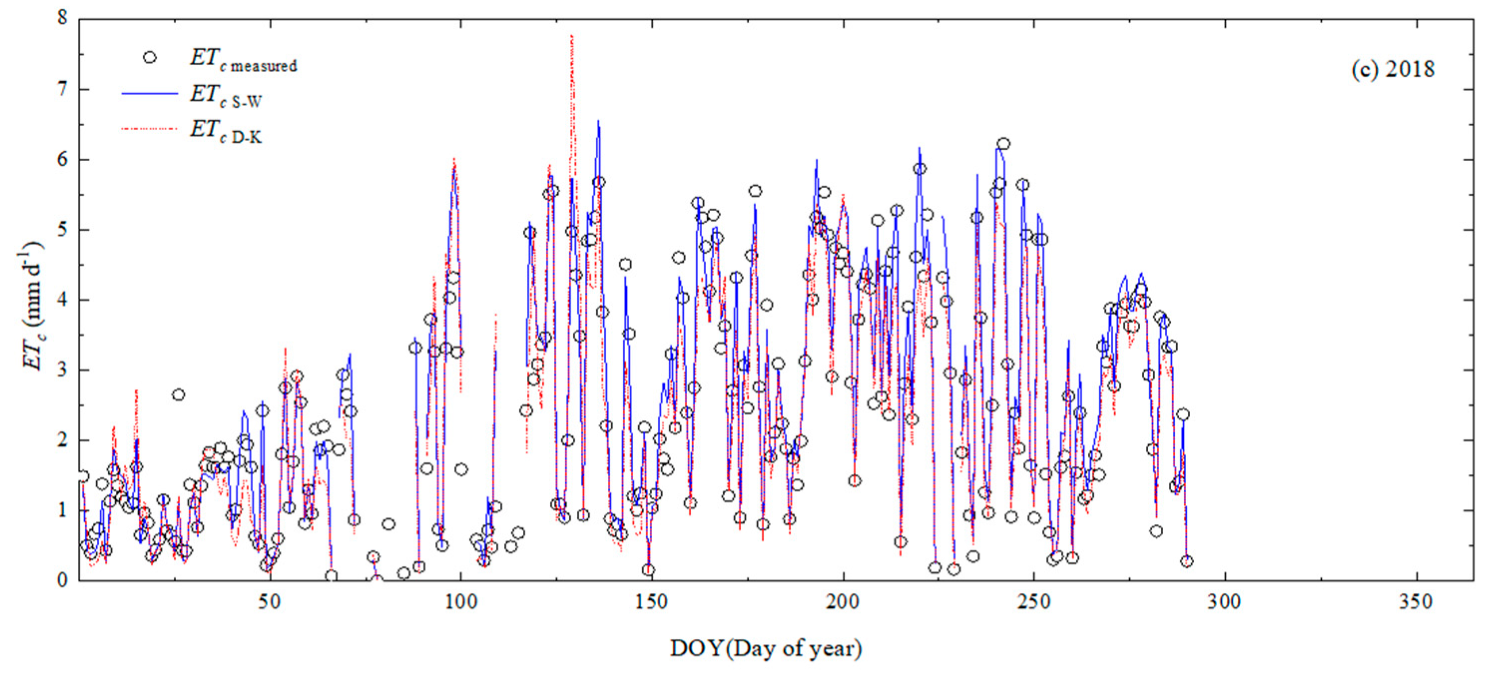
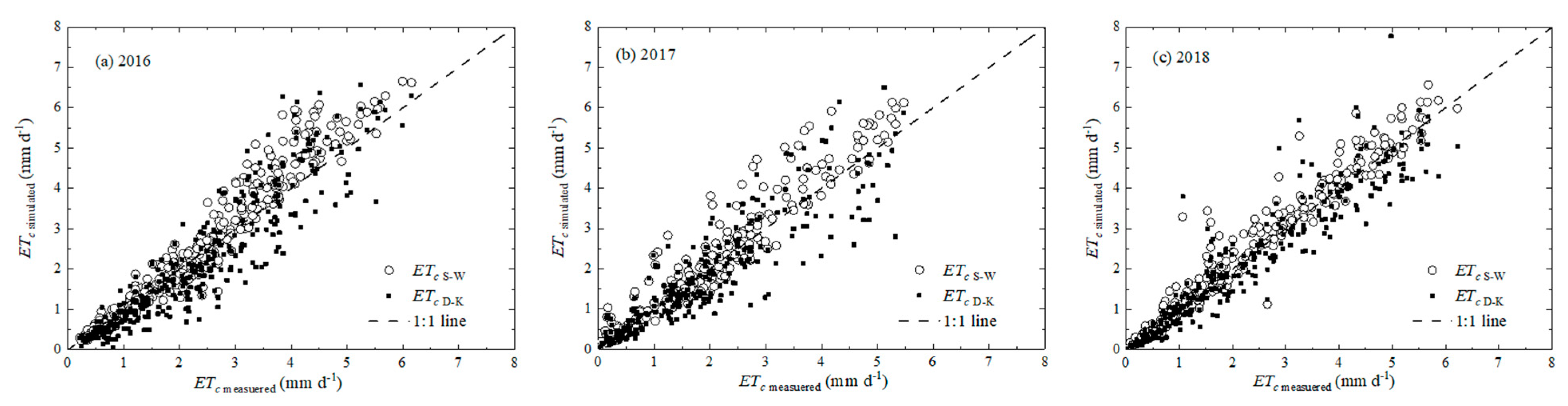
3.4. The Performance of Two Methods in ETc Simulation

Figure 5 showed the variations of estimated daily ETc by the S-W and D-K method and the measured values by Bowen ratio energy balance method in the tea field in 2016-2018. Results showed that both approaches had good performance in the estimation of ETc, except some overestimation of the D-K method at some unspecified date, e.g., 130 DOY of 2017 and 129 DOY of 2018 (Figure 5). From the regression analysis based on four years data (Figure 6), the average a and R2 were 1.07 and 0.97 for the S-W model, while the corresponding values were 0.97 and 0.95 for the D-K method, indicating that both methods had high correlations with the measured ETc. Table 1 showed the measured ETc varied from 2.01 to 2.40 mm d−1 with a mean of 2.21 mm d1 during the four years, while the measured ETc of 2017 was the lowest with an average value of 2.01 mm d−1. It can be explained that the most data (193–300 DOY) was lost in 2017. More statistical indices for evaluation of the accuracies of two approaches are shown in Table 1. The RMSE, MAE, and d were 0.45, 0.30 mm d−1, and 0.98 for the S-W model, while the corresponding values were 0.61, 0.43 mm d1, and 0.96 for the D-K method. Moreover, the biases were 0.06 and −0.03 for the S-W model and D-K method, respectively. The statistical indexes showed both approaches could accurately estimate the daily ETc in tea fields in southeast China, but the D-K method had a slightly poorer accuracy compared to the S-W model.
To further explore the differences of the S-W and D-K method in a separate estimation of T and E, the ratio of E to ETc simulated based on two methods was compared (Table 2). The simulated T were 1.89 mm d−1 in 2016, 1.69 mm d−1 in 2017, and 2.05 mm d−1 in 2018 by S-W model, while the corresponding E were 0.59, 0.47, and 0.52 mm d−1 for the three years, respectively. The E/ETc simulated by the S-W and D-K method were 21.93 % and 20.85 %, respectively. The E/ETc was declining year by year, and the highest value was 23.79 % in 2016. It can be explained that soil evaporation was related to the fraction of ground coverage when a smaller fraction of the soil surface was covered by the tea plants during the initial stage, which created a large wetted soil surface area that was exposed to sun radiation, and consequently higher soil evaporation. It is noteworthy that the difference between the E/ETc simulated by the S-W and D-K method was small (around 1%).

4. Discussion

4.1. Parametrization of S-W Model

Previous studies have highlighted the fact that the canopy resistance is the most sensitive factor compared to the other resistances in the S-W model due to its comprehensive consideration of meteorological factors, crop characteristics, and soil moisture conditions [10,11,22,48,49]. Therefore, accurate determination of the canopy resistance is particularly important in accurate estimation of ETc. Bao et al. [49] optimized a canopy resistance ( r s c ) sub-model of the S-W model and used a modified Ball–Berry model, including the empirical parameters estimated by the Monte Carlo algorithm for mobile dunes in China’s Horqin Sandy Land, with R2 and RMSE between the measurements and simulations as 0.83, 0.32 mm d−1, respectively. Liu et al. [50] improved the Jarvis-type r s c sub-model by incorporating a term of effective leaf area index and a function to reflect the influence of the specific soil moisture, to improve the accuracy of the S-W model for rice ETc in the Taihu lake region of China, with the R2 and RMSE were 0.945, 0.934 mm d1, respectively. In this study, we optimized KP-type r s c sub-model by a quadratic polynomial relationship based on the measured daily ETc in a tea field, with the R2 and RMSE at 0.97 and 0.45 mm d1, respectively. Compared to the previous studies, the S-W model parameterized by the present study achieved a higher accuracy. The main reason is that the KP-type r s c sub-model in this study was optimized with a best-fit quadratic polynomial relationship, not a linear function, which is more adaptive to the tea field.

4.2. Prediction of Crop Coefficients

As for perennial plants, the average Kc values (0.86) found for the tea plants in this study were lower than that reported by Pinho Sousa et al. [51] for acai palm (=1.08), Meijide et al. [52] for palm oil (=1.03), and Flumignan et al. [53] for coffee trees (=1.28 for ET0 < 3 mm d1, 0.98 for ET0 > 3 mm d1). The possible reason for this is that the Kc in this study was determined using the dataset in 2015, while the tea plants were transplanted into the field in March 2014, which means the values of Kc were at the initial stage of the tea plants. Many researchers found that the Kc was significantly related to LAI [54,55,56]. For example, Wang et al. [56] presented a linear relationship between the Kc and LAI with a good result (R2 ≥ 0.78, p < 0.01) in a grapevine ecosystem in the Nanhu Oasis of northwestern China. Singh Rawat et al. [55] reported that the Kc and LAI were in a strong relationship (second order polynomia, R2 = 0.98) in a semi-arid environment. Guo et al. [54] presented a cubic polynomial function, which was the best for simulating the relationship between the Kc and LAI for spring maize in the arid region of Northwest China. In this study, due to the slight variations of daily LAI of tea plants and the difficulties in the measurement, the LAI was not considered to simulate the changes of the Kc. Instead, it was found that the θswc was significant correlated to the daily Kc (R2 = 0.92, p < 0.01).

4.3. Comparison of Model Performance

The calculated statistical indices showed that the S-W and D-K method can estimate daily ETc with good accuracy, except some big discrepancies of the D-K method some days. It can be explained that there are some irregular days for collecting tea, which may affect the daily Kc. Gharsallah et al. [26] compared the S-W model and D-K method in a surface irrigated maize agro-ecosystem in Northern Italy, and showed that the S-W model provided good results for the entire agricultural season, including initial growing stage, while the D-K method with generalized crop coefficients overestimated the ETc, especially during the middle growth stage. Jiang et al. [27] compared the D-K and the S-W model in predicting daily ETc and its components of maize, and reported that daily ETc estimated by the S-W model was closer than by the D-K method to observed ETc by the eddy covariance system at whole growing stage, while the D-K method overestimated daily ETc at the initial and development stage in the arid region of northwest China. The principal reason for the poorer performance of the D-K method is that the tabulated Kcb adjusted with local data used for the simulations overestimated the actual, site-specific Kcb. Indeed, Gharsallah et al. [26] found that the Kc in mid-stage, even if adjusted to consider local conditions, was approximately 15% larger than the value derived from eddy covariance observations for maize grown in Northern Italy. However, Zhao et al. [19] showed that an opposite result to the D-K method performed better in in partitioning ETc than the S-W model, while the S-W model significantly underestimated E, especially around wetting events of a vineyard in an arid region of northwest China. Gong et al. [11] also showed that the D-K method performed better compared to the S-W model in estimating daily tomato ETc in greenhouses, while the S-W model overestimated ETc by 17.9% at initial stage and underestimated ETc by 16.6% at mid-stage in Henan province, China. The possible reasons for the S-W model having performed poorly are: (1) the r s c in the S-W model was normally parameterized by the Jarvis approach or the modified Jarvis approach, the effect of water stress was not considered in the r s c sub-model; (2) the r s s in the S-W model was parameterized using the θswc at certain range (20–40%), while θswc deviated from the range especially before or just after the wetting events, the r s s would not be parameterized by θswc accurately. Gong et al. [11] reported that the overestimation of S-W model at the initial stage was mainly due to the underestimation of r s c under the soil water stress condition. Additionally, many studies have proved that the r s c was the most sensitive variable compared to the other resistance in the S-W model [10,11,19,22].

4.4. Implications of the Modeling

As stated above, the establishment of the parameter sub-model played a crucial role in determining the performance of the S-W and D-K method [11]. The parameter sub-model should combine effects of local meteorological elements, crop growth conditions, and soil water status [19,22]. In this study, the parameter of r s c   and Kc sub-models were recalibrated by combining the influence of the meteorological elements and soil water status in the tea field. By integrating the r s c   and Kc sub-models into the S-W and D-K method, both methods had good performances in estimating ETc of the tea field. However, how the effect of tea plants growth on the performance of the S-W and D-K methods can be integrated still needs to be further investigated.
In agricultural ecosystems, the fractions of E and T in ETc are affected by soil and water management practices, and they have been used as indicators of crop water use efficiency (WUE) [57,58]. In this study, the range of E/ETc in the tea field simulated by the S-W and D-K method was 22.33–23.79%, 21.40–21.76%, 18.81–20.23% in 2016, 2017, 2018, respectively. Some researchers have used in situ techniques (e.g., lysimeter method, eddy covariance, heat pulse sensors, and sap flow methods) to obtain the fraction of E in ETc, and Wang et al. [58] obtained an E/ETc value of 19% using sap flow gauges (to measure T) and the weighing lysimeter (to measure ETc) in a maize field; Sauer et al. [59] observed a E/ETc range of 8 %–12 % in a narrow-row soybean field using the eddy covariance system (to measure ETc) and sap flow stem gauges (to measure T); Wagle et al. [60] collected high frequency (=10 Hz) time series eddy covariance system observations over a rainfed alfalfa, and reported that the average E/ETc was approximately 18–23% in central Oklahoma, USA. Compared to the reported values of E/ETc from previous literatures, there is still space to minimize E loses in the tea fields. Hence, based on the results simulated by the constructed S-W and D-K methods in this study, reducing a proper amount of irrigation water to decrease the soil evaporation at the growing season of tea plants is an advisable way for improving water use efficiency, especially at initial stages in 2016.

5. Conclusions

In this study, we evaluated the S-W and D-K method in estimating daily evapotranspiration (ETc) and its components of a tea field, using the measurements of ETc by Bowen ratio energy balance system for four years (2015–2018) in southeast China. The canopy resistance ( r s c ) in the S-W model was parameterized by a climatic resistance r * , with a quadratic polynomial relationship between r s c / r a and square root of r * / r a . The soil surface resistance ( r s s ) in the S-W model was parameterized by the soil water content (θswc) at the top layer. The measured crop coefficient (Kc) was defined as the ratio of measured ETc to ET0, basal crop coefficient (Kcb), and evaporation coefficient (Ke) in the D-K method was determined based on the measured meteorological data, LAI, and θswc data in the tea field.
Both the S-W and D-K method had good performances in estimating ETc of the tea field, with an average RMSE and R2 of 0.53 mm d−1 and 0.96, while the S-W model performed slightly better than the D-K method. The measured and simulated average daily ETc of the tea field was 2.21 mm d1 (Bowen ratio energy balance), 2.36 mm d1, and 2.14 mm d1 (S-W model and D-K method, respectively). The average ratios of E to ETc simulated by the S-W and D-K method were 21.93 % and 20.85 %, respectively. The above results indicated that the E should be estimated independently for tea fields to improve the accuracy of ETc modeling.

Author Contributions

H.Y. and C.Z. designed the research; S.H., L.L., S.Z., M.L. and B.Z. performed the experiment; S.H. drafted the original paper; H.Y., J.Z., C.Z. and G.W. revised the paper and polished the English. All authors have read and agreed to the published version of the manuscript.

Funding

This study has been financially supported by the Natural Science Foundation of China (41860863); The National Key R&D Program (Grant No. 2021YFC3201103); the Belt and Road Special Foundation of the State Key Laboratory of Hydrology-Water Resources and Hydraulic Engineering (2020nkzd01); Yinshanbeilu Grassland Eco-hydrology National Observation and Research Station, China Institute of Water Resources and Hydropower Research, Beijing 100038, China, Grant No. YSS2022011; the postdoctoral Research of Jiangsu Province (Bs510001); the Open Fund of High-tech Key Laboratory of Agricultural Equipment and Intelligentization of Jiangsu Province (No. JNZ201917); a project funded by the Priority Academic Program Development of Jiangsu Higher Education Institutions China.

Institutional Review Board Statement

Not applicable.

Informed Consent Statement

Informed consent was obtained from all subjects involved in the study.

Data Availability Statement

Not applicable.

Conflicts of Interest

The authors declare no conflict of interest and do not have any commercial or associative interest that represents a conflict of interest in connection with the work submitted.

References

  1. Xia, E.H.; Zhang, H.B.; Sheng, J.; Li, K.; Zhang, Q.J.; Kim, C.; Zhang, Y.; Liu, Y.; Zhu, T.; Li, W.; et al. The Tea Tree Genome Provides Insights into Tea Flavor and Independent Evolution of Caffeine Biosynthesis. Mol. Plant 2017, 10, 866–877. [Google Scholar] [CrossRef] [PubMed]
  2. Acquah, S.J.; Yan, H.F.; Zhang, C.; Wang, G.Q.; Zhao, B.S.; Wu, H.M.; Zhang, H.N. Application and evaluation of Stanghellini model in the determination of crop evapotranspiration in a naturally ventilated greenhouse. Int. J. Agric. Biol. Eng. 2018, 11, 95–103. [Google Scholar]
  3. Yan, H.F.; Acquah, S.J.; Zhang, C.; Wang, G.Q.; Huang, S.; Zhang, H.N.; Zhao, B.S.; Wu, H.M. Energy partitioning of greenhouse cucumber based on the application of Penman-Monteith and Bulk Transfer models. Agric. Water Manag. 2019, 217, 201–211. [Google Scholar] [CrossRef]
  4. Stanghellini, C. Transpiration of Greenhouse Crops: An Aid to Climate Management. Ph.D. Thesis, Agricultural University of Wageningen, Wageningen, The Netherlands, 1987; 150p. [Google Scholar]
  5. Qiu, R.J.; Kang, S.Z.; Du, T.S.; Tong, L.; Hao, X.M.; Chen, R.Q.; Chen, J.L.; Li, F.S. Effect of convection on the Penman–Monteith model estimates of transpiration of hot pepper grown in solar greenhouse. Sci. Hortic. 2013, 160, 163–171. [Google Scholar] [CrossRef]
  6. Liu, H.; Duan, A.W.; Li, F.S.; Sun, J.S.; Wang, Y.C.; Sun, C.T. Drip irrigation scheduling for tomato grown in solar greenhouse based on pan evaporation in North China Plain. J. Integr. Agric. 2013, 12, 520–531. [Google Scholar] [CrossRef]
  7. Villarreal-Guerrero, F.; Kacira, M.; Fitz-Rodrı´guez, E.; Kubota, C.; Giacomelli, G.A.; Linker, R.; Arbel, A. Comparison of three evapotranspiration models for a greenhouse cooling strategy with natural ventilation and variable high pressure fogging. Sci. Hortic. 2012, 134, 210–221. [Google Scholar] [CrossRef]
  8. Valdés-Gómez, H.; Ortega-Farías, S.; Argote, M. Evaluation of water requirements for a greenhouse tomato crop using the Priestley–Taylor method. Chil. J. Agric. Res. 2009, 69, 3–11. [Google Scholar]
  9. Qiu, R.J.; Du, T.S.; Kang, S.Z.; Chen, R.Q.; Wu, L.S. Assessing the SIM-Dual Kc model for estimating evapotranspiration of hot pepper grown in a solar greenhouse in Northwest China. Agric. Syst. 2015, 138, 1–9. [Google Scholar] [CrossRef]
  10. Li, X.Y.; Yang, P.; Ren, S.M.; Li, Y.K.; Liu, H.L.; Du, J.; Li, P.F.; Wang, C.Y.; Ren, L. Modeling cherry orchard evapotranspiration based on an improved dual-source model. Agric. Water Manag. 2010, 98, 12–18. [Google Scholar] [CrossRef]
  11. Gong, X.W.; Liu, H.; Sun, J.S.; Gao, Y.; Zhang, H. Comparison of Shuttleworth-Wallace model and dual crop coefficient method for estimating evapotranspiration of tomato cultivated in a solar greenhouse. Agric. Water Manag. 2019, 217, 141–153. [Google Scholar] [CrossRef]
  12. Huang, S.; Yan, H.F.; Zhang, C.; Wang, G.Q.; Acquah, S.J.; Yu, J.J.; Ma, J.M.; Li, L.L.; Opoku Darko, R. Modeling evapotranspiration for cucumber plants based on the Shuttleworth-Wallace model in a Venlo-type greenhouse. Agric. Water Manag. 2019, 228, 105861. [Google Scholar] [CrossRef]
  13. Shuttleworth, W.J.; Wallace, J.S. Evaporation from sparse crops-an energy combination theory. Q. J. R. Meteorol. Soc. 1985, 111, 839–855. [Google Scholar] [CrossRef]
  14. Allen, R.G.; Pereira, L.S.; Raes, D.; Smith, M. Crop Evapotranspiration Guidelines for Computing Crop Water Requirements, Irrigation and Drainage; FAO: Roe, Italy, 1998; Volume 56, 300p. [Google Scholar]
  15. Ding, R.S.; Kang, S.Z.; Zhang, Y.Q.; Hao, X.M.; Tong, L.; Du, T.S. Partitioning evapotranspiration into soil evaporation and transpiration using a modified dual crop coefficient model in irrigated maize field with ground-mulching. Agric. Water Manag. 2013, 127, 85–96. [Google Scholar] [CrossRef]
  16. Poblete-Echeverría, C.A.; Ortega-Farias, S.O. Evaluation of single and dual crop coefficients over a drip-irrigated Merlot vineyard (Vitis vinifera L.) using combined measurements of sap flow sensors and an eddy covariance system. Aust. J. Grape Wine Res. 2013, 19, 249–260. [Google Scholar] [CrossRef]
  17. Zhu, G.F.; Su, Y.H.; Li, X.; Zhang, K.; Li, C.B. Estimating actual evapotranspiration from an alpine grassland on Qinghai–Tibetan plateau using a two-source model and parameter uncertainty analysis by Bayesian approach. J. Hydrol. 2013, 476, 42–51. [Google Scholar] [CrossRef]
  18. Zhu, G.F.; Li, X.; Su, Y.H.; Zhang, K.; Bai, Y.; Ma, J.Z.; Li, C.B.; Hu, X.L.; He, J.H. Simultaneously assimilating multivariate data sets into the two-source evapotranspiration model by Bayesian approach: Application to spring maize in an arid region of northwestern China. Geosci. Model Dev. 2014, 7, 1467–1482. [Google Scholar] [CrossRef]
  19. Zhao, P.; Li, S.E.; Li, F.S.; Du, T.; Tong, L.; Kang, S.Z. Comparison of dual crop coefficient method and Shuttleworth-Wallace model in evapotranspiration partitioning in a vineyard of northwest China. Agric. Water Manag. 2015, 160, 41–56. [Google Scholar] [CrossRef]
  20. Kool, D.; Agam, N.; Lazarovitch, N.; Heitman, J.L.; Sauer, T.J.; Ben-Gal, A. A review of approaches for evapotranspiration partitioning. Agric. For. Meteorol. 2014, 184, 56–70. [Google Scholar] [CrossRef]
  21. Iritza, Z.; Lindrotha, A.; Heikinheimob, M.; Grellea, A.; Kellnerc, E. Test of a modified Shuttleworth–Wallace estimate of boreal forest evaporation. Agric. For. Meteorol. 1999, 98, 605–619. [Google Scholar] [CrossRef]
  22. Ortega-Farias, S.; Poblete-Echeverría, C.; Brisson, N. Parameterization of a two-layer model for estimating vineyard evapotranspiration using meteorological measurements. Agric. For. Meteorol. 2010, 150, 276–286. [Google Scholar] [CrossRef]
  23. Zhang, B.Z.; Kang, S.Z.; Li, F.S.; Zhang, L. Comparison of three evapotranspiration models to Bowen ratio-energy balance method for a vineyard in an arid desert region of northwest China. Agric. For. Meteorol. 2008, 148, 1629–1640. [Google Scholar] [CrossRef]
  24. Yan, H.F.; Oue, H. Application of the two-layer model for predicting transpiration from the rice canopy and water surface evaporation beneath the canopy. J. Agric. Meteorol. 2011, 67, 89–97. [Google Scholar] [CrossRef] [Green Version]
  25. Liu, S.Y.; Wang, Y.K.; Wei, X.D.; Wei, X.G.; Wang, X.; Zhang, L.L. Measured and estimated evapotranspiration of jujube (ziziphus jujuba) forests in the loess plateau, china. Int. J. Agric. Biol. 2013, 15, 811–819. [Google Scholar]
  26. Gharsallah, O.; Facchi, A.; Gandolfi, C. Comparison of six evapotranspiration models for a surface irrigated maize agro-ecosystem in Northern Italy. Agric. Water Manag. 2013, 130, 119–130. [Google Scholar] [CrossRef]
  27. Jiang, X.L.; Kang, S.Z.; Tong, L.; Li, S.E.; Ding, R.S.; Du, T.S. Modeling evapotranspiration and its components of maize for seed production in an arid region of northwest China using a dual crop coefficient and multisource models. Agric. Water Manag. 2019, 222, 105–117. [Google Scholar] [CrossRef]
  28. Anderson, R.G.; Alfieri, J.G.; Tirado-Corbalá, R.; Gartung, J.; McKee, L.G.; Prueger, J.H.; Wang, D.; Ayars, J.E.; Kustas, W.P. Assessing FAO-56 dual crop coefficients using eddy covariance flux partitioning. Agric. Water Manag. 2017, 179, 92–102. [Google Scholar] [CrossRef]
  29. Zhao, N.N.; Liu, Y.; Cai, J.B.; Paredes, P.; Rosa, R.D.; Pereira, L.S. Dual crop coefficient modelling applied to the winter wheat–summer maize crop sequence in North China Plain: Basal crop coefficients and soil evaporation component. Agric. Water Manag. 2013, 117, 93–105. [Google Scholar] [CrossRef]
  30. Miao, Q.F.; Rosa, R.D.; Shi, H.B.; Paredes, P.; Zhu, L.; Dai, J.X.; Gonçalves, J.M.; Pereira, L.S. Modeling water use, transpiration and soil evaporation of spring wheat–maize and spring wheat–sunflower relay intercropping using the dual crop coefficient approach. Agric. Water Manag. 2016, 165, 211–229. [Google Scholar] [CrossRef]
  31. Rosa, R.D.; Ramos, T.B.; Pereira, L.S. The dual Kc approach to assess maize and sweet sorghum transpiration and soil evaporation under saline conditions: Application of the SIMDualKc model. Agric. Water Manag. 2016, 177, 77–94. [Google Scholar] [CrossRef]
  32. Yan, H.F.; Zhang, C.; Peng, G.J.; Darko, R.O.; Cai, B. Modelling canopy resistance for estimating latent heat flux at a tea field in South China. Exp. Agric. 2017, 54, 563–576. [Google Scholar] [CrossRef]
  33. Beer, C.; Ciais, P.; Reichstein, M.; Baldocchi, D.; Law, B.E.; Papale, D.; Soussana, J.F.; Ammann, C.; Buchmann, N.; Frank, D.; et al. Temporal and among-site variability of inherent water use efficiency at the ecosystem level. Glob. Biogeochem. Cycles 2009, 23, GB2018. [Google Scholar] [CrossRef]
  34. Katerji, N.; Perrier, A. Modelisation de l’evapotranspiration reelle d’une parcelle de luzerne: Role d’un coefficient cultural. Agronomie 1983, 3, 513–521. [Google Scholar] [CrossRef]
  35. Monteith, J.L.; Szeicz, G.; Waggoner, P.E. The measurement and control of stomatal resistance in the field. J. Appl. Ecol. 1965, 2, 345–355. [Google Scholar] [CrossRef]
  36. Perez, P.J.; Lecina, S.; Castellvi, F.; Martinez-Cob, A.; Villalobos, F.J. A simple parameterization of bulk canopy resistance from climatic variables for estimating hourly evapotranspiration. Hydrol. Process. 2006, 20, 515–532. [Google Scholar] [CrossRef]
  37. Yan, H.F.; Shi, H.B.; Oue, H.; Zhang, C.; Xue, Z.; Cai, B.; Wang, G.Q. Modeling bulk canopy resistance from climatic variables for predicting hourly evapotranspiration of maize and buckwheat. Meteorol. Atmos. Phys. 2015, 127, 305–312. [Google Scholar] [CrossRef]
  38. Perrier, A. Physical study of evapotranspiration in natural conditions. I. Evaporation and balance of energy of natural surfaces. Ann. Agron. 1975, 26, 1–18. [Google Scholar]
  39. Perrier, A. Physical study of evapotranspiration in natural conditions. III. Actual and potential evapotranspiration of canopies. Ann. Agron. 1975, 26, 229–243. [Google Scholar]
  40. ASCE-EWRI. The ASCE Standardized Reference Evapotranspiration Equation; Report by the Task Committee on Standardization of Reference Evapotranspiration; ASCE: Reston, VA, USA, 2005; 204p, ISBN 078440805X. [Google Scholar]
  41. Zhao, P.; Kang, S.Z.; Li, S.E.; Ding, R.S.; Tong, L.; Du, T.S. Seasonal variations in vineyard ET partitioning and dual crop coefficients correlate with canopy development and surface soil moisture. Agric. Water Manag. 2018, 197, 19–33. [Google Scholar] [CrossRef]
  42. Zhang, C.; Yan, H.F.; Takase, K.; Oue, H. Comparison of the soil physical properties and hydrological processes in two different forest type catchments. Water Resour. 2016, 43, 225–237. [Google Scholar] [CrossRef]
  43. Katerji, N.; Rana, G.; Fahed, S. Parameterizing canopy resistance using mechanistic and semi-empirical estimates of hourly evapotranspiration: Critical evaluation for irrigated crops in the Mediterranean. Hydrol. Process. 2011, 25, 117–129. [Google Scholar] [CrossRef]
  44. Liu, G.S.; Liu, Y.; Hafeez, M.; Xu, D.; Vote, C. Comparison of two methods to derive time series of actual evapotranspiration using eddy covariance measurements in the southeastern Australia. J. Hydrol. 2012, 454–455, 1–6. [Google Scholar] [CrossRef]
  45. He, B.; Oue, H.; Oki, T. Estimation of Hourly Evapotranspiration in Arid Regions by a Simple Parameterization of Canopy Resistance. J. Agric. Meteorol. 2009, 65, 39–46. [Google Scholar] [CrossRef]
  46. Rana, G.; Katerji, N.; Mastorilli, M.; EI Moujabber, M.; Brisson, N. Validation of a model of actual evapotranspiration for water stresses soybeans. Agric. For. Meteorol. 1997, 86, 215–224. [Google Scholar] [CrossRef]
  47. Rosa, R.D.; Paredes, P.; Rodrigues, G.C.; Fernando, R.M.; Alves, I.; Pereira, L.S.; Allen, R.G. Implementing the dual crop coefficient approach in interactive software: 2. Model testing. Agric. Water Manag. 2012, 103, 62–77. [Google Scholar] [CrossRef]
  48. Yan, H.F.; Zhang, C.; Gerrits, M.C.; Acquah, S.J.; Zhang, H.N.; Wu, H.M.; Zhao, B.S.; Huang, S.; Fu, H.W. Parametrization of aerodynamic and canopy resistances for modeling evapotranspiration of greenhouse cucumber. Agric. For. Meteorol. 2018, 262, 370–378. [Google Scholar] [CrossRef]
  49. Bao, Y.Z.; Duan, L.M.; Liu, T.X.; Tong, X.; Wang, G.Q.; Lei, H.M.; Zhang, L.; Singh, V.P. Simulation of evapotranspiration and its components for the mobile dune using an improved dual-source model in semi-arid regions. J. Hydrol. 2021, 592, 125796. [Google Scholar] [CrossRef]
  50. Liu, X.Y.; Xu, J.Z.; Wang, W.G.; Lv, Y.P.; Li, Y.W. Modeling rice evapotranspiration under water-saving irrigation condition: Improved canopy-resistance-based. J. Hydrol. 2020, 590, 125435. [Google Scholar] [CrossRef]
  51. Pinho Sousa, D.; Fernandes, T.F.S.; Tavares, L.B.; Silva Farias, V.D.; Lima, M.J.A.; Nunes, H.G.G.C.; Costa, D.L.P.; Ortega-Farias, S.; Oliveira Ponte Souza, P.J. Estimation of evapotranspiration and single and dual crop coefficients of acai palm in the Eastern Amazon (Brazil) using the Bowen ratio system. Irrig. Sci. 2021, 39, 5–22. [Google Scholar] [CrossRef]
  52. Meijide, A.; Röll, A.; Fan, Y.; Herbst, M.; Niu, F.; Tiedemann, F.; June, T.; Rauf, A.; Hölscher, D.; Knohl, A. Controls of water and energy fluxes in oil palm plantations: Environmental variables and oil palm age. Agric. For. Meteorol. 2017, 239, 71–85. [Google Scholar] [CrossRef]
  53. Flumignan, D.L.; Faria, R.T.; Cavenaghi Prete, C.E. Evapotranspiration components and dual crop coefficients of coffee trees during crop production. Agric. Water Manag. 2011, 98, 791–800. [Google Scholar] [CrossRef]
  54. Guo, H.; Li, S.E.; Kang, S.Z.; Du, T.S.; Tong, L.; Hao, X.M.; Ding, R.S. Crop coefficient for spring maize under plastic mulch based on 12-year eddy covariance observation in the arid region of Northwest China. J. Hydrol. 2020, 588, 125108. [Google Scholar] [CrossRef]
  55. Singh Rawat, K.; Kumar Singh, S.; Bala, A.; Szabó, S. Estimation of crop evapotranspiration through spatial distributed crop coefficient in a semi-arid environment. Agric. Water Manag. 2019, 213, 922–933. [Google Scholar] [CrossRef]
  56. Wang, S.T.; Zhu, G.F.; Xia, D.S.; Ma, J.Z.; Han, T.; Ma, T.; Zhang, K.; Shang, S.S. The characteristics of evapotranspiration and crop coefficients of an irrigated vineyard in arid Northwest China. Agric. Water Manag. 2019, 212, 388–398. [Google Scholar] [CrossRef]
  57. Agam, N.; Evett, S.R.; Tolk, J.A.; Kustas, W.P.; Colaizzi, P.D.; Alfieri, J.G.; Mckee, L.G.; Copeland, K.S.; Howell, T.A.; Chavez, J.L. Evaporative loss from irrigated interrows in a highly advective semi-arid agricultural area. Adv. Water Resour. 2012, 50, 20–30. [Google Scholar] [CrossRef]
  58. Wang, Y.Y.; Horton, R.; Xue, X.Z.; Ren, T.S. Partitioning evapotranspiration by measuring soil water evaporation with heat-pulse sensors and plant transpiration with sap flow gauges. Agric. Water Manag. 2021, 252, 106883. [Google Scholar] [CrossRef]
  59. Sauer, T.J.; Singer, J.W.; Prueger, J.H.; Desutter, T.M.; Hatfield, J.L. Radiation balance and evaporation partitioning in a narrow-row soybean canopy. Agric. For. Meteorol. 2007, 145, 206–214. [Google Scholar] [CrossRef]
  60. Wagle, P.; Skaggs, T.H.; Gowda, P.H.; Northup, B.K.; Neel, J.P.S. Flux variance similarity-based partitioning of evapotranspiration over a rainfed alfalfa field using high frequency eddy covariance data. Agric. For. Meteorol. 2020, 285–286, 107907. [Google Scholar] [CrossRef]
Figure 1. Daily variations of net radiation (Rn, W m−2), air temperature (Ta, °C), water vapor pressure deficit (VPD, KPa), and wind speed (u, m s−1) at the tea field in 2015–2018.
Agriculture 12 01392 g001
Figure 2. The daily variation of experimental values of r s c / r a and ( r * / r a )0.5 in the tea field during the spring shoots (from 1 March through 31 May) in 2015.
Agriculture 12 01392 g002
Figure 3. The daily variation of the local measured crop coefficient (Kc) and volumetric soil water content (θswc) at 10 cm below the soil surface in the tea field in 2015 (a); the relationship between Kc and θswc in 2015 (b).
Agriculture 12 01392 g003
Figure 4. The variations of basal crop coefficient (Kcb), soil evaporation coefficient (Ke) in the tea field (Kcb-cal is calculated from Equation (23); Kcb-FAO is recommended by FAO-56).
Agriculture 12 01392 g004
Figure 5. Variations of measured and simulated ETc by the S-W and D-K method in 2016–2018.
Agriculture 12 01392 g005aAgriculture 12 01392 g005b
Figure 6. Comparison of observed and simulated daily ETc by the S-W and D-K method in 2016–2018. Dash line represents 1:1 line.
Agriculture 12 01392 g006
Table 1. Statistical analysis of measured and estimated daily evapotranspiration (ETc, mm d1) by the S-W and D-K method in 2016–2018.
YearModelETc-MimulatedETc-MeasuredaR2RMSEMAEdBias
2016S-W2.332.221.070.980.420.270.980.05
D-K2.171.000.950.590.430.96−0.02
2017S-W2.162.011.080.970.510.340.970.07
D-K1.950.960.930.670.470.94−0.03
2018S-W2.582.401.060.980.430.280.980.07
D-K2.310.950.960.580.390.97−0.04
AverageS-W2.362.211.070.970.450.300.980.06
D-K2.140.970.950.610.430.96−0.03
Note: a is the coefficients of regression; R2 is the coefficient of determination; RMSE is the root mean square error (mm d−1); MAE is the mean absolute error (mm d−1); d is the index of agreement.
Table 2. Models simulated values of tea plants transpiration (T) and soil evaporation (E) in 2016–2018.
YearModelT (mm d1)E (mm d1)E/ETc
2016S-W1.890.5923.79%
D-K2.470.7122.33%
2017S-W1.690.4721.76%
D-K2.350.6421.40%
2018S-W2.050.5220.23%
D-K2.590.618.81%
AverageS-W1.880.5321.93%
D-K2.470.6520.85%
Publisher’s Note: MDPI stays neutral with regard to jurisdictional claims in published maps and institutional affiliations.

